Chapter 5: Joint Probability Distributions and Random...
32
Chapter 5: Joint Probability Distributions and Ran- dom Samples Curtis Miller 2018-06-13 Introduction We may naturally inquire about collections of random vari- ables that are related to each other in some way. For instance, we may record an individual’s height and weight, calling these random vari- ables X and Y, and ask if these are correlated, uncorrelated, or even independent characteristics, and describe a probability model that accounts for the relationship in these two characteristics. Additionally, we may have a large collection of random variables, say X 1 , X 2 ,..., X n which will be used to estimate some essential quantity of a distribution, such as the mean μ. We compute some quantity based on this collection of random variables, such as ¯ X = 1 n ∑ n i=1 X i , or any other T = T(X 1 ,..., X n ). This quantity, dependent on random variables, is itself a random variable, and we call it a statistic. Being a statistic it has its own probability distribution, with its own mean and variance and cdf, and we can use the distribution of the statistic to make statements about the process that generated the original dataset X 1 ,..., X n . It is here when probability theory begins to turn into statistical theory. Section 1: Jointly Distributed Random Variables Suppose X and Y are two discrete random variables. Their joint probability mass function is described below: This can be used to compute ((X, Y) ∈ A) for an event A: From this we can compute the marginal probability mass func- tions, p X ( x) and p Y (y), for X and Y respectively.
Transcript of Chapter 5: Joint Probability Distributions and Random...
Chapter 5: Joint Probability Distributions and Ran-dom SamplesCurtis Miller
2018-06-13
Introduction
We may naturally inquire about collections of random vari-ables that are related to each other in some way. For instance, we mayrecord an individual’s height and weight, calling these random vari-ables X and Y, and ask if these are correlated, uncorrelated, or evenindependent characteristics, and describe a probability model thataccounts for the relationship in these two characteristics.
Additionally, we may have a large collection of random variables,say X1, X2, . . . , Xn which will be used to estimate some essentialquantity of a distribution, such as the mean µ. We compute somequantity based on this collection of random variables, such as X =1n ∑n
i=1 Xi, or any other T = T(X1, . . . , Xn). This quantity, dependenton random variables, is itself a random variable, and we call it astatistic. Being a statistic it has its own probability distribution, withits own mean and variance and cdf, and we can use the distributionof the statistic to make statements about the process that generatedthe original dataset X1, . . . , Xn. It is here when probability theorybegins to turn into statistical theory.
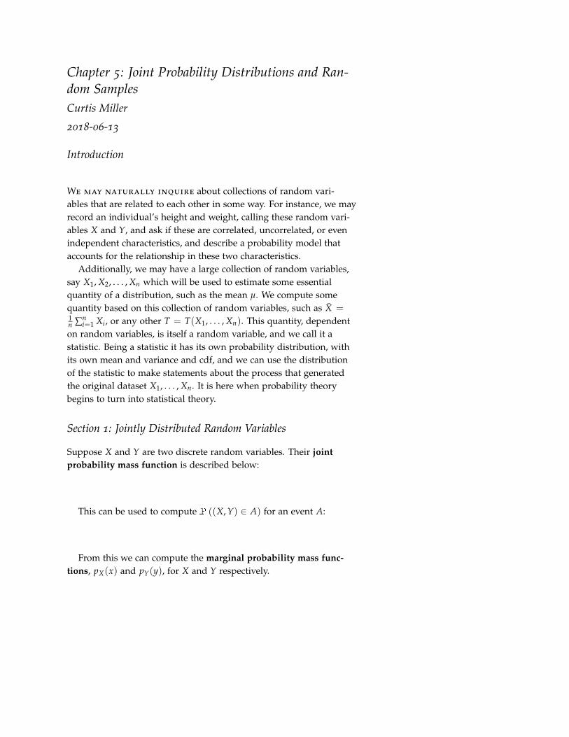
Section 1: Jointly Distributed Random Variables
Suppose X and Y are two discrete random variables. Their jointprobability mass function is described below:
This can be used to compute P ((X, Y) ∈ A) for an event A:
From this we can compute the marginal probability mass func-tions, pX(x) and pY(y), for X and Y respectively.
chapter 5: joint probability distributions and random samples 2
These represent the probability distribution of X and Y respec-tively regardless of what value the other rv takes.
We can also compute what is known as the conditional probabil-ity mass function of Y given X = x, which represents the probabilitydistribution of Y when we know that X = x. The conditional proba-bility mass function of X given Y = y is defined in a similar manner.
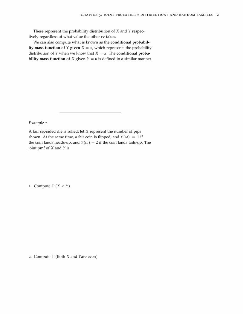
Example 1
A fair six-sided die is rolled; let X represent the number of pipsshown. At the same time, a fair coin is flipped, and Y(ω) = 1 ifthe coin lands heads-up, and Y(ω) = 2 if the coin lands tails-up. Thejoint pmf of X and Y is
1. Compute P (X < Y).
2. Compute P (Both X and Yare even)
chapter 5: joint probability distributions and random samples 3
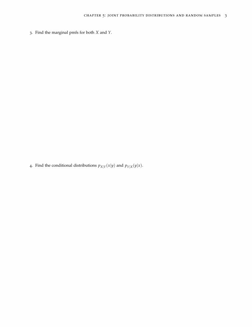
3. Find the marginal pmfs for both X and Y.
4. Find the conditional distributions pX|Y(x|y) and pY|X(y|x).
chapter 5: joint probability distributions and random samples 4
library(discreteRV)
##
## Attaching package: ’discreteRV’
## The following object is masked from ’package:base’:
##
## %in%
library(magrittr) # Adds the %>% operator
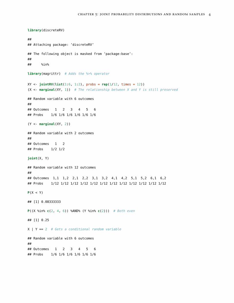
XY <- jointRV(list(1:6, 1:2), probs = rep(1/12, times = 12))
(X <- marginal(XY, 1)) # The relationship between X and Y is still preserved
## Random variable with 6 outcomes
##
## Outcomes 1 2 3 4 5 6
## Probs 1/6 1/6 1/6 1/6 1/6 1/6
(Y <- marginal(XY, 2))
## Random variable with 2 outcomes
##
## Outcomes 1 2
## Probs 1/2 1/2
joint(X, Y)
## Random variable with 12 outcomes
##
## Outcomes 1,1 1,2 2,1 2,2 3,1 3,2 4,1 4,2 5,1 5,2 6,1 6,2
## Probs 1/12 1/12 1/12 1/12 1/12 1/12 1/12 1/12 1/12 1/12 1/12 1/12
P(X < Y)
## [1] 0.08333333
P((X %in% c(2, 4, 6)) %AND% (Y %in% c(2))) # Both even
## [1] 0.25
X | Y == 2 # Gets a conditional random variable
## Random variable with 6 outcomes
##
## Outcomes 1 2 3 4 5 6
## Probs 1/6 1/6 1/6 1/6 1/6 1/6
chapter 5: joint probability distributions and random samples 5
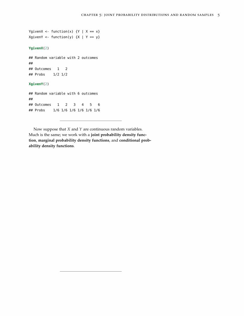
YgivenX <- function(x) {Y | X == x}
XgivenY <- function(y) {X | Y == y}
YgivenX(2)
## Random variable with 2 outcomes
##
## Outcomes 1 2
## Probs 1/2 1/2
XgivenY(2)
## Random variable with 6 outcomes
##
## Outcomes 1 2 3 4 5 6
## Probs 1/6 1/6 1/6 1/6 1/6 1/6
Now suppose that X and Y are continuous random variables.Much is the same; we work with a joint probability density func-tion, marginal probability density functions, and conditional prob-ability density functions.
chapter 5: joint probability distributions and random samples 6
Example 2
A company sells bags of “deluxe” mixed nuts, containing almonds,cashews, and peanuts. One bag is five pounds, and the joint pdf forthe amount of almonds X and cashews Y in the bag (in pounds) isgiven below:
(We don’t need to worry about the amount of peanuts; this issimply 5− X−Y and thus is completely determined given X and Y.)
The region on which the pdf is illustrated below:
1. Customers buying bags of “deluxe” mixed nuts complain when60% of the nuts in the bag are peanuts. Compute the probabilitythis occurs.
chapter 5: joint probability distributions and random samples 7
2. Find the marginal distributions of X and Y. Use this to computeE [X], E [Y], Var (X), and Var (Y).
3. Find the conditional pdfs fX|Y(x|y) and fY|X(y|x). Use this tocompute P (X > 2|Y = 2).
chapter 5: joint probability distributions and random samples 8
We say that two random variables X and Y are independent if
Example 3
Are the random variables in the previous two example independent?Explain why or why not.
chapter 5: joint probability distributions and random samples 9
independent(X, Y) # For Example 1
## [1] TRUE
We can generalize our definitions from two to n rvs, X1, . . . , Xn.
We say that X1, . . . , Xn are independent if for every subset Xi1 , . . . , Xikof the collection, we have
If X1, . . . , Xn are independent and each has the same pmf/pdfthat X1, . . . , Xn are independent and identically distributed, oftenabbreviated i.i.d..1 1 This is a typical assumption about a
dataset in statistics.
Example 4
Compute P (min{X1, ..., Xn} ≥ x) if X1, . . . , Xn are i.i.d..
chapter 5: joint probability distributions and random samples 10
We can generalize the binomial distribution we saw before thethe multinomial distribution. We have r categories, and a singleobservation belongs to category i with probability pi. We count howmany observations belong to category i; this gives Xi. Then the vector(X1, . . . , Xr) follows the multinomial distribution, or (X1, . . . , Xr) ∼MULTINOM(p1, . . . , pr)2, and we have the pmf 2 The binomial distribution is a par-
ticular instance of the multinomialdistribution, when r = 2. We omit thecount of tails, which we may call X2, asit’s redundant information given X1.
Section 2: Expected Values, Covariance, and Correlation
Expectations involving two random variables are defined similarly tothe univariate cases.
Example 5
Reconsider the random variables in Examples 1 and 2. ComputeE [XY] for both cases.

chapter 5: joint probability distributions and random samples 11
chapter 5: joint probability distributions and random samples 12
E(X * Y) # For Example 1’s random variables
## [1] 5.25
One measure of the relationship between two random variables isthe covariance.
The covariance is positive if the two random variables tend to belarge together, while the covariance is negative if one rv tends to belarge when the other tends to be small. If Cov (X, Y) = 0, then X andY are uncorrelated.3 3 Due to the relationship between
the covariance and the variance,we sometimes see the notationCov (X, Y) = σXY .
We also have the following shortcut formula for the covariance:
It’s obtained in a similar manner to shortcut formulas found forcomputing Var (X).4 4 From this it’s clear that Cov (X, X) =
Var (X).Notice that the covariance is not insensitive to the units of the ran-dom variable; in fact, we can compute the covariance Cov (aX + b, cY + d):
Changing the units changes the covariance. A unit-free measure ofthe relationship between X and Y is the correlation.5 5 The usual Greek letter representing
correlation is ρ.
The correlation is 1 if there is a perfect positive linear relationshipbetween X and Y, -1 if there is a perfect negative linear relationship,and 0 if there is no linear relationship between X and Y.6 Thus |ρ| 6 Notice the emphasis on the word
“linear”; there can be a relationshipbetween X and Y that would make theircorrelation small yet there could still bea strong nonlinear relationship linkingthe two variables.
determines the strength of the relationship7 between X and Y and
7 We can classify the strength of therelationship between rvs using com-pletely arbitrary cutoffs; specifically, wecould say that if |ρ| < 0.3 there is nonotable correlation, if |ρ| > 0.7 there isa strong correlation, and otherwise thecorrelation is weak.
sign(ρ) determines the direction of the relationship.8
8 There is a sample statistic for estimat-ing ρ from paired data (x1, yi):
r =1
sxsy(n− 1)
n
∑i=1
(xi − x)(yi − y)
The interpretation is the same. We donot discuss the sample statistic in thiscourse.
Example 6
Compute the covariance and correlation for the random variablesmentioned in Examples 1 and 2.
chapter 5: joint probability distributions and random samples 13
# For Example 1
(sigma_xy <- E(X * Y) - E(X) * E(Y))
## [1] 0
If X and Y are independent, then Cov (X, Y) = 0.9 The converse is 9 As a consequence, we can equivalentlysay that E [XY] = E [X]E [Y] when Xand Y are idependent.
not true in general, as the following example shows.
Example 7
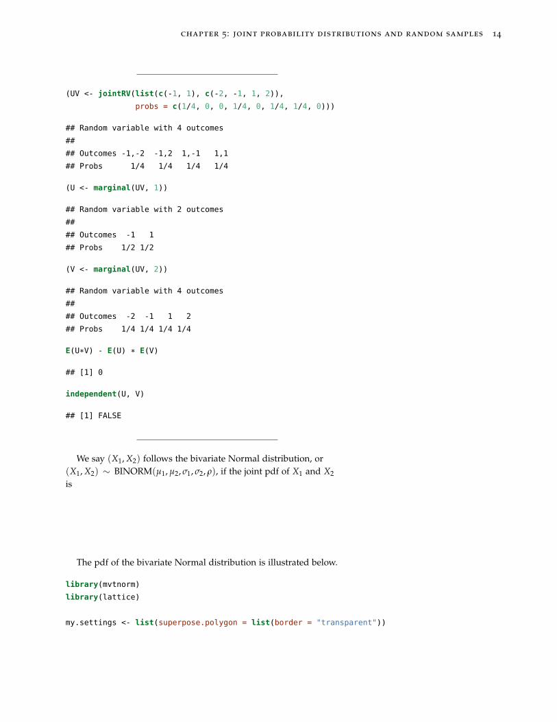
The point (U, V) is equally likely to be any of the points in thesample space S = {(1, 1), (1,−1), (−1, 2), (−1,−2)}. ComputeCov (U, V). Are U and V independent?
chapter 5: joint probability distributions and random samples 14
(UV <- jointRV(list(c(-1, 1), c(-2, -1, 1, 2)),
probs = c(1/4, 0, 0, 1/4, 0, 1/4, 1/4, 0)))
## Random variable with 4 outcomes
##
## Outcomes -1,-2 -1,2 1,-1 1,1
## Probs 1/4 1/4 1/4 1/4
(U <- marginal(UV, 1))
## Random variable with 2 outcomes
##
## Outcomes -1 1
## Probs 1/2 1/2
(V <- marginal(UV, 2))
## Random variable with 4 outcomes
##
## Outcomes -2 -1 1 2
## Probs 1/4 1/4 1/4 1/4
E(U*V) - E(U) * E(V)
## [1] 0
independent(U, V)
## [1] FALSE
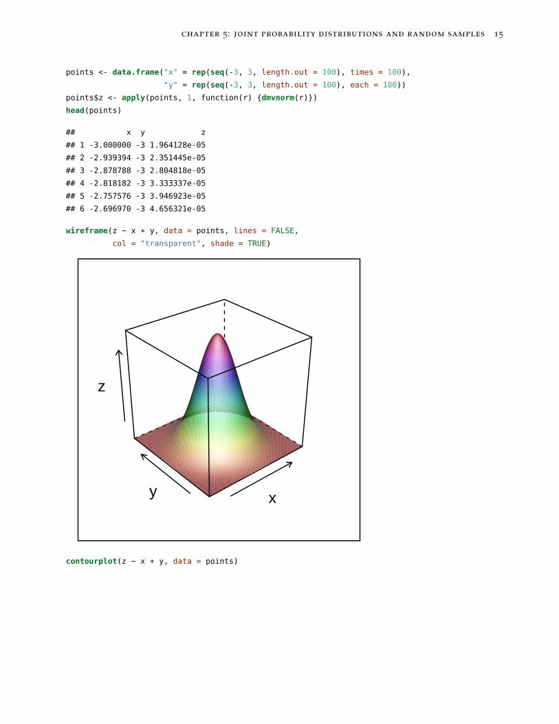
We say (X1, X2) follows the bivariate Normal distribution, or(X1, X2) ∼ BINORM(µ1, µ2, σ1, σ2, ρ), if the joint pdf of X1 and X2
is
The pdf of the bivariate Normal distribution is illustrated below.
library(mvtnorm)
library(lattice)
my.settings <- list(superpose.polygon = list(border = "transparent"))
chapter 5: joint probability distributions and random samples 15
points <- data.frame("x" = rep(seq(-3, 3, length.out = 100), times = 100),
"y" = rep(seq(-3, 3, length.out = 100), each = 100))
points$z <- apply(points, 1, function(r) {dmvnorm(r)})
head(points)
## x y z
## 1 -3.000000 -3 1.964128e-05
## 2 -2.939394 -3 2.351445e-05
## 3 -2.878788 -3 2.804818e-05
## 4 -2.818182 -3 3.333337e-05
## 5 -2.757576 -3 3.946923e-05
## 6 -2.696970 -3 4.656321e-05
wireframe(z ~ x * y, data = points, lines = FALSE,
col = "transparent", shade = TRUE)
xy
z
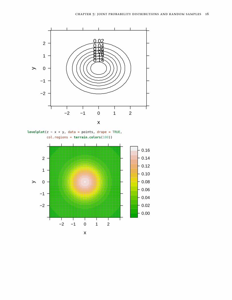
contourplot(z ~ x * y, data = points)
chapter 5: joint probability distributions and random samples 16
x
y
−2
−1
0
1
2
−2 −1 0 1 2
0.020.040.060.080.100.120.14
levelplot(z ~ x * y, data = points, drape = TRUE,
col.regions = terrain.colors(100))
x
y
−2
−1
0
1
2
−2 −1 0 1 2
0.00
0.02
0.04
0.06
0.08
0.10
0.12
0.14
0.16
chapter 5: joint probability distributions and random samples 17
If you were to slice the pdf in any direction, the resulting plotwould be another Normal distribution. Specifically, the marginal dis-tributions fX1(x1) and fX2(x2) are Normal distributions, and condi-tional distributions fX1|X2
(x1|x2) and fX2|X1(x2|x1) are all all Normal
distributions.
We have E [X1] = µ1, E [X2] = µ2, SD (X1) = σ1, SD (X2) = σ2,and Corr (X1, X2) = ρ. Crucially, when (X1, X2) follows a bivariateNormal distribution, Cov (X1, X2) does imply independence!10 10 This is not the same as saying that
if two random variables are Normallydistributed and uncorrelated theyare independent. Joint normalitydoes not follow from the normalityof the marginal distributions; forexample, if we choose Z1 ∼ N(0, 1)and Z2 = SZ1 with P (S = 1) =P (S = −1) = 1
2 , then Z2 ∼ N(0, 1), andthe marginal distributions of (Z1, Z2)are thus standard Normal distributions,and Cov (Z1, Z2) = 0. However, Z1 andZ2 are obviously not independent sinceif we know Z1 then we know Z2 differsfrom Z1 by at most a sign.
Example 8
Let HC represent the height of a son and HF the height of the son’sfather (in inches). Suppose
(HC, HF) ∼ BINORM(69.2, 69.2, 2.6, 2.6, 0.4)
1. What are the marginal distributions of HC and HF?
chapter 5: joint probability distributions and random samples 18
2. Suppose a person’s father is 78 inches tall. Find an equal-tailed11 11 In general, when we say an intervalis equal-tailed, we mean that the prob-ability that the random variable is toosmall to be in the region is equal to theprobability that the random variableis too large. We need this restriction inorder to have a unique solution; other-wise, there could be an infinite numberof solutions.
interval such that the probability the child’s height is in this inter-val is 0.95.
chapter 5: joint probability distributions and random samples 19
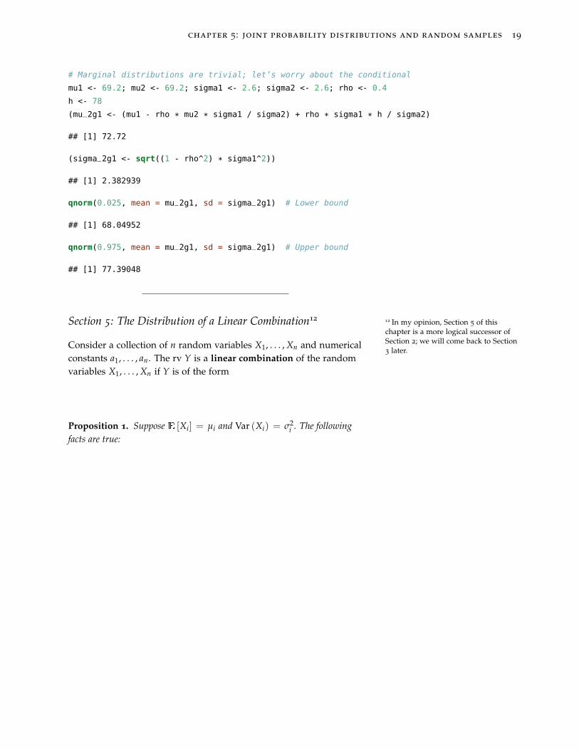
# Marginal distributions are trivial; let’s worry about the conditional
mu1 <- 69.2; mu2 <- 69.2; sigma1 <- 2.6; sigma2 <- 2.6; rho <- 0.4
h <- 78
(mu_2g1 <- (mu1 - rho * mu2 * sigma1 / sigma2) + rho * sigma1 * h / sigma2)
## [1] 72.72
(sigma_2g1 <- sqrt((1 - rho^2) * sigma1^2))
## [1] 2.382939
qnorm(0.025, mean = mu_2g1, sd = sigma_2g1) # Lower bound
## [1] 68.04952
qnorm(0.975, mean = mu_2g1, sd = sigma_2g1) # Upper bound
## [1] 77.39048
Section 5: The Distribution of a Linear Combination1212 In my opinion, Section 5 of thischapter is a more logical successor ofSection 2; we will come back to Section3 later.
Consider a collection of n random variables X1, . . . , Xn and numericalconstants a1, . . . , an. The rv Y is a linear combination of the randomvariables X1, . . . , Xn if Y is of the form
Proposition 1. Suppose E [Xi] = µi and Var (Xi) = σ2i . The following
facts are true:
chapter 5: joint probability distributions and random samples 20
Thus we have the important property about expectations; theyare linear operators, to use linear algebra language. The variance isnot a linear operator (although it is a sublinear operator), but thecovariance is a bilinear operator (linear in both its arguments).
Corollary 1. Suppose X1 and X2 are two independent random variables.Then:
We can weaken the independence assumption to simply beinguncorrelated and the variance computation will still be true.
Proposition 2. Suppose X1 and X2 are two Normal random variables.Then
Corollary 2. A linear combination of Normal random variables also followsa Normal distribution.
Example 9
Suppose X1, . . . , Xn are i.i.d. random variables. Compute the ex-pected value, variance, and standard deviation of X = 1
n ∑ni=1 Xi.
chapter 5: joint probability distributions and random samples 21
Example 10
Suppose X1, . . . , Xn are i.i.d. random variables. Compute the ex-pected value, variance, and standard deviation of T = ∑n
i=1 Xi
There are several random variables where we know the distribu-tion of sums of those random variables. Below is a summary:
Section 3: Statistics and Their Distributions
We will call the collection X1, . . . , Xn a random sample if it consistsof i.i.d. random variables. We will call any quantity we can computefrom a random sample a statistic. Before the dataset is observed, astatistic is a random quantity, with its own distribution, referred to asthe sampling distribution; statistics in this random state are usuallyreferred to using upper-case letters, while the observed statistic (afterwe have a dataset) is usually referred to using lower-case letters.
Examples of statistics include:
chapter 5: joint probability distributions and random samples 22
Example 11
Let X1, . . . , Xn be i.i.d.r.v. with X1 ∼ Ber(p). What is the samplingdistribution of X?
Example 12
Let X1, . . . , Xn be i.i.d.r.v. with X1 ∼ N(µ, σ). What is the samplingdistribution of X? Use the sampling distribution to find an intervalsuch that P (l(X) ≤ µ ≤ u(X)) = 1− α.
chapter 5: joint probability distributions and random samples 23
One approach to finding information about the sampling distri-bution of statistics is to use simulations. We generate K randomsamples of size n, X1,k, . . . , Xn,k, k ∈ [K]. For each sample we computethe statistic of interest T(X1,k, . . . , Xn,k) = Tk, and then study therandom sample T1, . . . , TK.
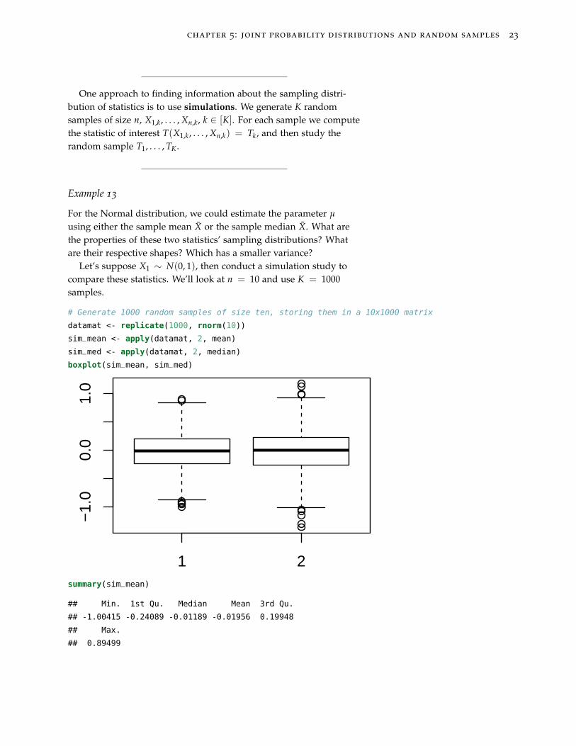
Example 13
For the Normal distribution, we could estimate the parameter µ
using either the sample mean X or the sample median X. What arethe properties of these two statistics’ sampling distributions? Whatare their respective shapes? Which has a smaller variance?
Let’s suppose X1 ∼ N(0, 1), then conduct a simulation study tocompare these statistics. We’ll look at n = 10 and use K = 1000samples.
# Generate 1000 random samples of size ten, storing them in a 10x1000 matrix
datamat <- replicate(1000, rnorm(10))
sim_mean <- apply(datamat, 2, mean)
sim_med <- apply(datamat, 2, median)
boxplot(sim_mean, sim_med)
1 2
−1.
00.
01.
0
summary(sim_mean)
## Min. 1st Qu. Median Mean 3rd Qu.
## -1.00415 -0.24089 -0.01189 -0.01956 0.19948
## Max.
## 0.89499
chapter 5: joint probability distributions and random samples 24
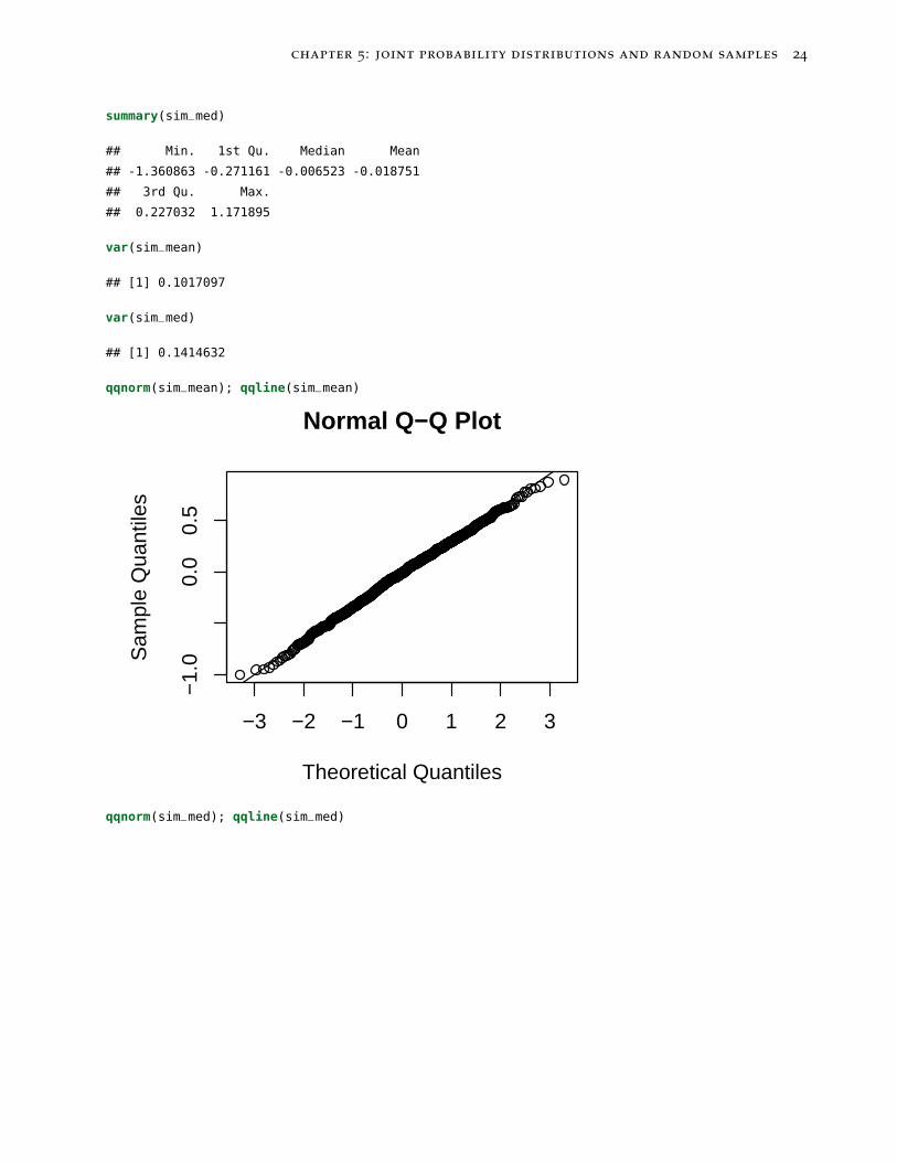
summary(sim_med)
## Min. 1st Qu. Median Mean
## -1.360863 -0.271161 -0.006523 -0.018751
## 3rd Qu. Max.
## 0.227032 1.171895
var(sim_mean)
## [1] 0.1017097
var(sim_med)
## [1] 0.1414632
qqnorm(sim_mean); qqline(sim_mean)
−3 −2 −1 0 1 2 3
−1.
00.
00.
5
Normal Q−Q Plot
Theoretical Quantiles
Sam
ple
Qua
ntile
s
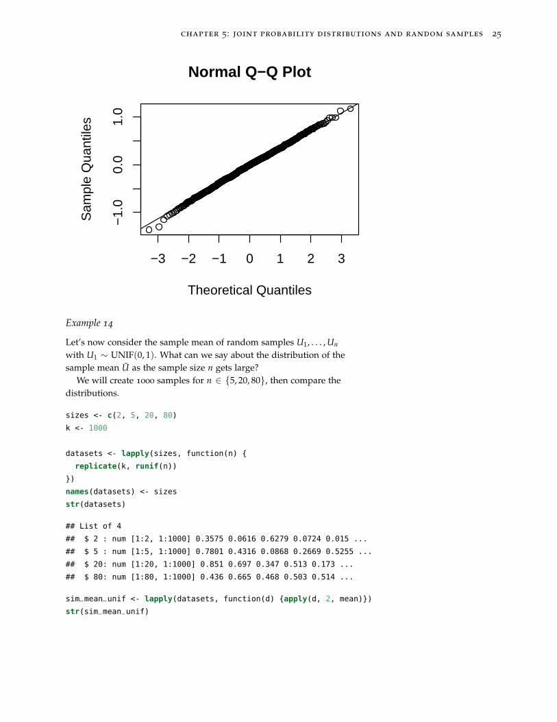
qqnorm(sim_med); qqline(sim_med)
chapter 5: joint probability distributions and random samples 25
−3 −2 −1 0 1 2 3
−1.
00.
01.
0
Normal Q−Q Plot
Theoretical Quantiles
Sam
ple
Qua
ntile
s
Example 14
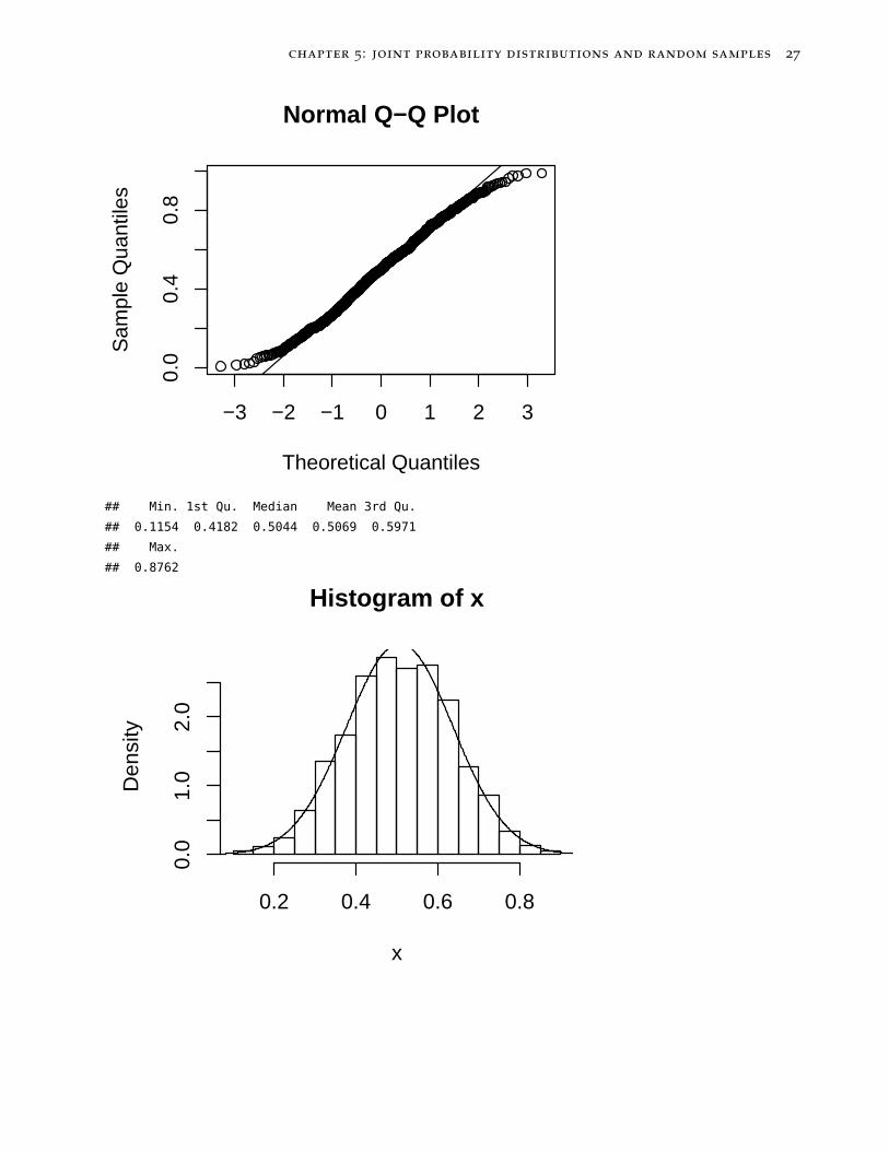
Let’s now consider the sample mean of random samples U1, . . . , Un
with U1 ∼ UNIF(0, 1). What can we say about the distribution of thesample mean U as the sample size n gets large?
We will create 1000 samples for n ∈ {5, 20, 80}, then compare thedistributions.
sizes <- c(2, 5, 20, 80)
k <- 1000
datasets <- lapply(sizes, function(n) {
replicate(k, runif(n))
})
names(datasets) <- sizes
str(datasets)
## List of 4
## $ 2 : num [1:2, 1:1000] 0.3575 0.0616 0.6279 0.0724 0.015 ...
## $ 5 : num [1:5, 1:1000] 0.7801 0.4316 0.0868 0.2669 0.5255 ...
## $ 20: num [1:20, 1:1000] 0.851 0.697 0.347 0.513 0.173 ...
## $ 80: num [1:80, 1:1000] 0.436 0.665 0.468 0.503 0.514 ...
sim_mean_unif <- lapply(datasets, function(d) {apply(d, 2, mean)})
str(sim_mean_unif)
chapter 5: joint probability distributions and random samples 26
## List of 4
## $ 2 : num [1:1000] 0.21 0.35 0.479 0.228 0.804 ...
## $ 5 : num [1:1000] 0.418 0.716 0.779 0.407 0.491 ...
## $ 20: num [1:1000] 0.48 0.377 0.504 0.568 0.483 ...
## $ 80: num [1:1000] 0.513 0.495 0.492 0.5 0.503 ...
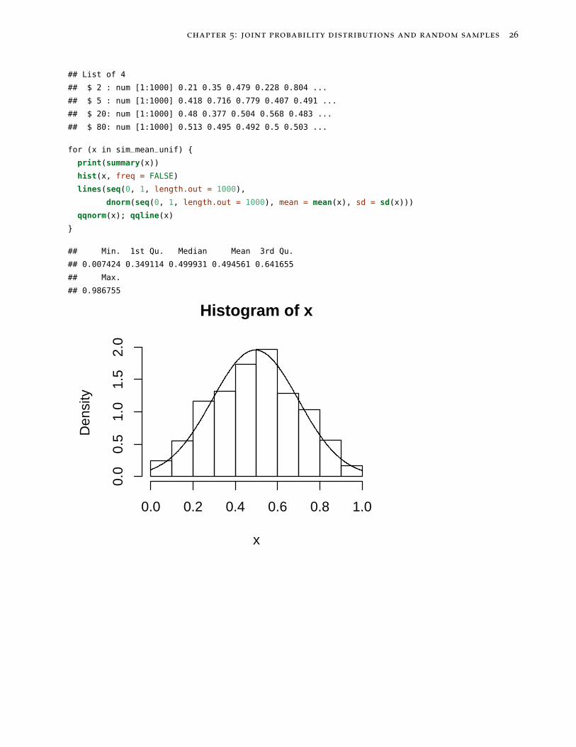
for (x in sim_mean_unif) {
print(summary(x))
hist(x, freq = FALSE)
lines(seq(0, 1, length.out = 1000),
dnorm(seq(0, 1, length.out = 1000), mean = mean(x), sd = sd(x)))
qqnorm(x); qqline(x)
}
## Min. 1st Qu. Median Mean 3rd Qu.
## 0.007424 0.349114 0.499931 0.494561 0.641655
## Max.
## 0.986755
Histogram of x
x
Den
sity
0.0 0.2 0.4 0.6 0.8 1.0
0.0
0.5
1.0
1.5
2.0
chapter 5: joint probability distributions and random samples 27
−3 −2 −1 0 1 2 3
0.0
0.4
0.8
Normal Q−Q Plot
Theoretical Quantiles
Sam
ple
Qua
ntile
s
## Min. 1st Qu. Median Mean 3rd Qu.
## 0.1154 0.4182 0.5044 0.5069 0.5971
## Max.
## 0.8762
Histogram of x
x
Den
sity
0.2 0.4 0.6 0.8
0.0
1.0
2.0
chapter 5: joint probability distributions and random samples 28
−3 −2 −1 0 1 2 3
0.2
0.4
0.6
0.8
Normal Q−Q Plot
Theoretical Quantiles
Sam
ple
Qua
ntile
s
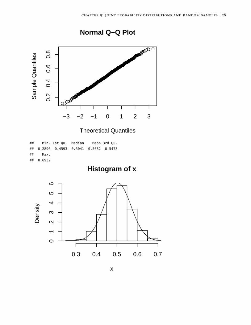
## Min. 1st Qu. Median Mean 3rd Qu.
## 0.2896 0.4593 0.5041 0.5032 0.5473
## Max.
## 0.6932
Histogram of x
x
Den
sity
0.3 0.4 0.5 0.6 0.7
01
23
45
6
chapter 5: joint probability distributions and random samples 29
−3 −2 −1 0 1 2 3
0.3
0.4
0.5
0.6
0.7
Normal Q−Q Plot
Theoretical Quantiles
Sam
ple
Qua
ntile
s
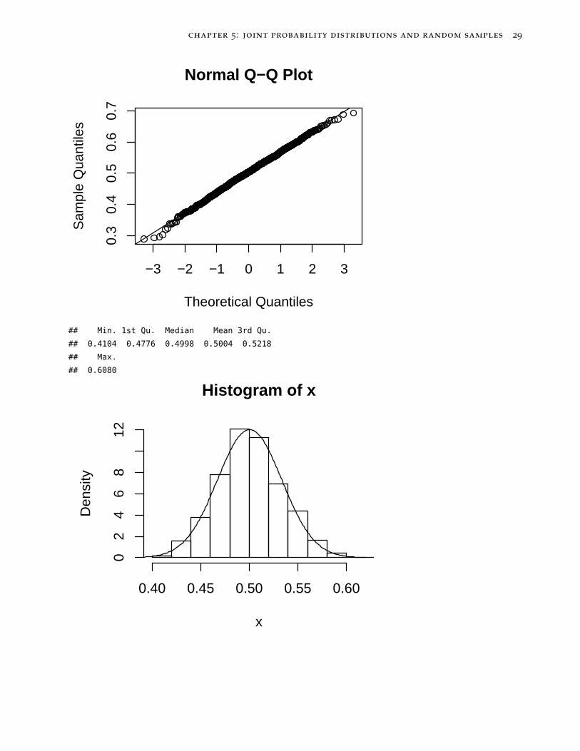
## Min. 1st Qu. Median Mean 3rd Qu.
## 0.4104 0.4776 0.4998 0.5004 0.5218
## Max.
## 0.6080
Histogram of x
x
Den
sity
0.40 0.45 0.50 0.55 0.60
02
46
812
chapter 5: joint probability distributions and random samples 30
−3 −2 −1 0 1 2 3
0.45
0.55
Normal Q−Q Plot
Theoretical Quantiles
Sam
ple
Qua
ntile
s
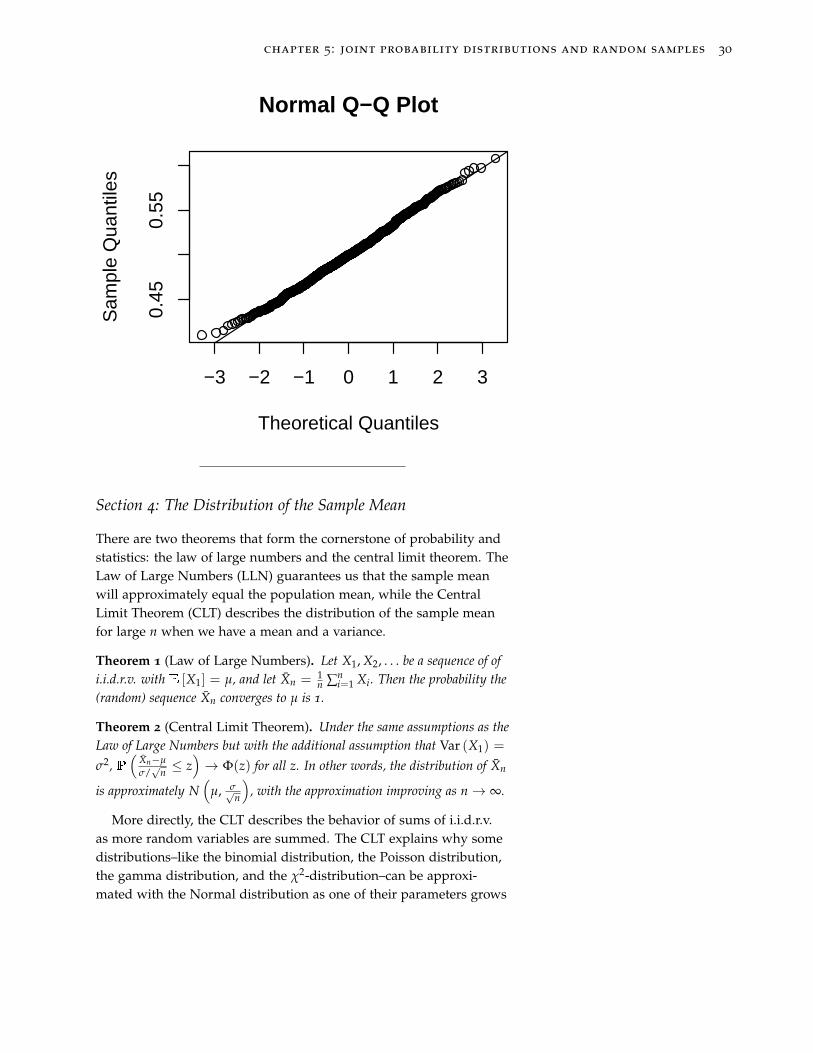
Section 4: The Distribution of the Sample Mean
There are two theorems that form the cornerstone of probability andstatistics: the law of large numbers and the central limit theorem. TheLaw of Large Numbers (LLN) guarantees us that the sample meanwill approximately equal the population mean, while the CentralLimit Theorem (CLT) describes the distribution of the sample meanfor large n when we have a mean and a variance.
Theorem 1 (Law of Large Numbers). Let X1, X2, . . . be a sequence of ofi.i.d.r.v. with E [X1] = µ, and let Xn = 1
n ∑ni=1 Xi. Then the probability the
(random) sequence Xn converges to µ is 1.
Theorem 2 (Central Limit Theorem). Under the same assumptions as theLaw of Large Numbers but with the additional assumption that Var (X1) =
σ2, P(
Xn−µ
σ/√
n ≤ z)→ Φ(z) for all z. In other words, the distribution of Xn
is approximately N(
µ, σ√n
), with the approximation improving as n→ ∞.
More directly, the CLT describes the behavior of sums of i.i.d.r.v.as more random variables are summed. The CLT explains why somedistributions–like the binomial distribution, the Poisson distribution,the gamma distribution, and the χ2-distribution–can be approxi-mated with the Normal distribution as one of their parameters grows
chapter 5: joint probability distributions and random samples 31
large; these distributions can be interpreted as the distributions ofsums of i.i.d.r.v.13 and thus the CLT applies.14 13 Specifically: BIN(n, p) is the sum of
n Ber(p) r.v.s; POI(n) is the sum of nPOI(1) r.v.s; GAMMA(α, n) is the sumof n EXP(α) r.v.s; and χ2(n) is the sumof n χ2(1) r.v.s.14 The CLT requires that Var (X1) < ∞;if this does not hold, the CLT no longerapplies and its conclusion may not evenbe true.
Thanks to the CLT, we can describe the distribution of the samplemean without worrying about the exact distribution of the under-lying data if the sample size n is large enouch15, since the CLT says
15 In general it’s safe to use the CLT ifn > 30.
that the initial distribution is eventually “forgotten” by the samplemean.
Example 15
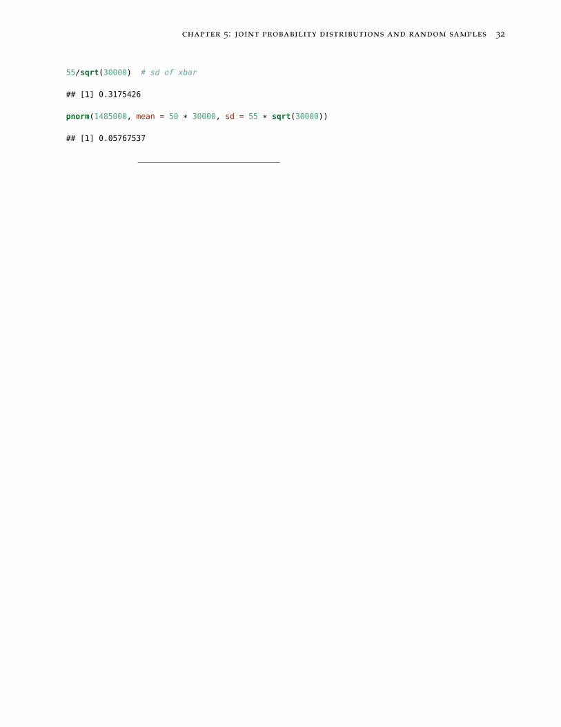
The average customer visiting a grocery store spends X dollars,where E [X] = 50 and SD (X) = 55.16 Every month about 30,000
16 Notice X is non-negative butSD (X) > E [X]. This can happenwith skewed distributions.
purchases are made at the grocery store.
1. What will be the (approximate) distribution of the average pur-chase, X?
2. What is the (approximate) probability that the revenue of thegrocery store in a month is less than $1,485,000
chapter 5: joint probability distributions and random samples 32
55/sqrt(30000) # sd of xbar
## [1] 0.3175426
pnorm(1485000, mean = 50 * 30000, sd = 55 * sqrt(30000))
## [1] 0.05767537