Chapter 24 - Handbook of Optics -...
50
P d A d R d T d 3 OPTICAL MEASUREMENTS
Transcript of Chapter 24 - Handbook of Optics -...
P d A d R d T d 3
OPTICAL MEASUREMENTS
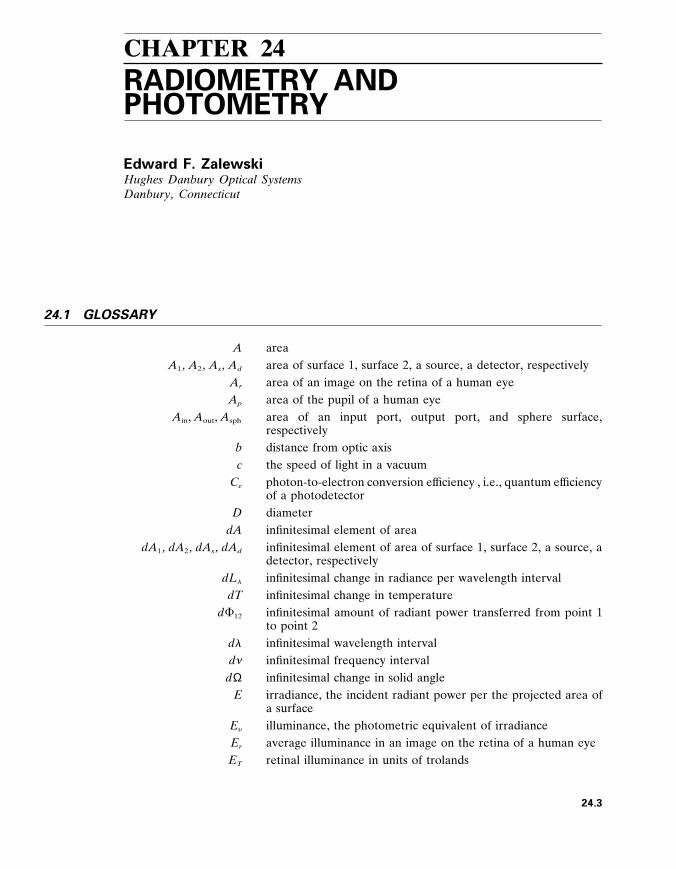
CHAPTER 24 RADIOMETRY AND PHOTOMETRY
Edward F . Zalewski Hughes Danbury Optical Systems Danbury , Connecticut
2 4 . 1 GLOSSARY
A area A 1 , A 2 , A s , A d area of surface 1 , surface 2 , a source , a detector , respectively
A r area of an image on the retina of a human eye A p area of the pupil of a human eye
A i n , A o u t , A s p h area of an input port , output port , and sphere surface , respectively
b distance from optic axis c the speed of light in a vacuum
C e photon-to-electron conversion ef ficiency , i . e ., quantum ef ficiency of a photodetector
D diameter dA infinitesimal element of area
dA 1 , dA 2 , dA s , dA d infinitesimal element of area of surface 1 , surface 2 , a source , a detector , respectively
dL l infinitesimal change in radiance per wavelength interval dT infinitesimal change in temperature
d F 1 2 infinitesimal amount of radiant power transferred from point 1 to point 2
d l infinitesimal wavelength interval d … infinitesimal frequency interval
d Ω infinitesimal change in solid angle E irradiance , the incident radiant power per the projected area of
a surface E y illuminance , the photometric equivalent of irradiance E r average illuminance in an image on the retina of a human eye E T retinal illuminance in units of trolands
24 .3
24 .4 OPTICAL MEASUREMENTS
E T ( l ) photopic retinal illuminance from a monochromatic source in trolands
E 9 T ( l ) scotoptic retinal illuminance from a monochromatic source in trolands
E r l retinal spectral irradiance in absolute units : W nm 2 1 m 2 2
f focal length
f 4 F -number
g fraction of light lost through the input and output ports of an averaging sphere
h Planck’s constant
h s , h d object (source) height , image (detector) height
I radiant intensity , the emitted or reflected radiant power per solid angle
i photoinduced current from a radiation detector
I y luminous intensity , the photometric equivalent of radiant intensity
k Boltzmann’s constant
K m luminous ef ficacy (i . e ., lumen-to-watt conversion factor) for photopic vision
K 9 m luminous ef ficacy for scotopic vision
K a b nonlinearity correction factor for a photodetector
L radiance , the radiant power per projected area and solid angle
L 1 2 radiance from point 1 into the direction of point 2
L a , L b radiance in medium a , in medium b
L e radiance within the human eye
L l radiance per wavelength interval
L … radiance per frequency interval
L y luminance , the photometric equivalent of radiance
L y ( l ) luminance of a monochromatic light source
M exitance , the emitted or reflected radiant power per the projected area of a source
m mean value
N photon flux , the number of photons per second
n index of refraction
n a , n b index of refraction in medium a , in medium b
n e index of refraction of the ocular medium of the human eye
n s , n d index of refraction in the object (i . e ., source) region , in the image (i . e ., detector) region
N l photon flux per wavelength interval
N … photon flux per frequency interval
N E l photon flux irradiance on the retina of a human eye
Q radiant energy
RADIOMETRY AND PHOTOMETRY 24 .5
Q l radiant energy per wavelength interval
Q … radiant energy per frequency interval
R responsivity of a photodetector , i . e ., electrical signal out per radiant signal in
r radius
r s , r d , r s p h radius of a source , detector , sphere , respectively
R ( l ) spectral (i . e ., per wavelength interval) responsivity of a photodetector
s distance
s 1 2 length of the light ray between points 1 and 2
s s d length of the light ray between points on the source and detector
s p r distance from the pupil to the retina in a human eye
T absolute temperature
t time
U photon dose , the total number of photons
V ( l ) spectral luminous ef ficiency function (i . e ., peak normalized human visual spectral responsivity) for photopic vision
V 9 ( l ) spectral luminous ef ficiency function for scotopic vision
w width
x i the i th sample in a set of measurements
a absorptance , fraction of light absorbed
b a , b b angle of incidence or refraction
g absorption coef ficient of a solute
d angle of rotation between crossed polarizers
» emittance of a blackbody simulator
E e tendue
h total number of sample measurements
θ s , θ d angle between the light ray and the normal to a point on the surface of a source , of a detector
θ 1 , θ 2 angle between the light ray and the normal to a surface at point 1 , at point 2
k concentration of a solute
l wavelength
… frequency
r fraction of light scattered or reflected
s standard deviation
s m standard deviation of the mean
τ transmittance , radiant signal out per radiant signal into a material
τ ( l ) spectral (i . e ., per wavelength interval) transmittance
τ e ( l ) spectral transmittance of the ocular medium of the human eye
24 .6 OPTICAL MEASUREMENTS
F radiant power or equivalently radiant flux f half angle subtended by a cone
F i n , F o u t incoming radiant power , outgoing radiant power F r luminous flux at the retina of the human eye F l radiant power per wavelength interval F … radiant power per frequency interval F y photopic luminous flux , radiant power detectable by photopic
human vision F 9 y scotopic luminous flux , radiant power detectable by scotopic
human vision Ω solid angle , a portion of the area on the surface of a sphere per
the square of the sphere radius Ω a , Ω b solid angle in medium a , in medium b
2 4 . 2 INTRODUCTION
Radiometry is the measurement of the energy content of electromagnetic radiation fields and the determination of how this energy is transferred from a source , through a medium , and to a detector . The results of a radiometric measurement are usually obtained in units of power , i . e ., in watts . However , the result may also be expressed as photon flux (photons per second) or in units of energy (joules) or dose (photons) . The measurement of the ef fect of the medium on the transfer of radiation , i . e ., the absorption , reflection , or scatter , is usually called spectrophotometry and will not be covered here . Rather , the assumption is made here that the radiant power is transferred through a lossless medium .
Traditional radiometry assumes that the propagation of the radiation field can be treated using the laws of geometrical optics . That is , the radiant energy is assumed to be transported along the direction of a ray and interference or dif fraction ef fects can be ignored . In those situations where interference or dif fraction ef fects are significant , the flow of energy will be in directions other than along those of the geometrical rays . In such cases , the ef fect of interference or dif fraction can often be treated as a correction to the result obtained using geometrical optics . This assumption is equivalent to assuming that the energy flow is via an incoherent radiation field . This assumption is widely applicable since most radiation sources are to a large degree incoherent . For a completely rigorous treatment of radiant energy flow , the degree of coherence of the radiation must be considered via a formalism based on the theory of electromagnetism as derived from Maxwell’s equations . 1 , 2 This complexity is not necessary for most of the problems encountered in radiometry .
In common practice , radiometry is divided according to regions of the spectrum in which the same experimental techniques can be used . Thus , vacuum ultraviolet radi- ometry , intermediate-infrared radiometry , far-infrared radiometry , and microwave radi- ometry are considered separate fields , and all are distinguished from radiometry in the visible and near-visible optical spectral region .
The reader should note that there is considerable confusion regarding the nomencla- tures of the various radiometries . The terminology for radiometry that we have inherited is dictated not only by its historical origin , 3 but also by that of related fields of study . By the late 1700s , techniques were developed to measure light using the human eye as a null detector in comparisons of sources . At about the same time , radiant heating ef fects were studied with liquid-in-glass thermometers and actinic (i . e ., chemical) ef fects of solar radiation were studied by the photoinduced decomposition of silver compounds into
RADIOMETRY AND PHOTOMETRY 24 .7
metallic silver . The discovery of infrared radiation in 1800 and ultraviolet radiation in 1801 stimulated a great deal of ef fort to study the properties of these radiations . However , the only practical detectors of ultraviolet radiation at that time were the actinic ef fects—for infrared radiation it was thermometers and for visible radiation it was human vision . Thus actinometry , radiometry , and photometry became synonymous with studies in the ultraviolet , infrared , and visible spectral regions . Seemingly independent fields of study evolved and even today there is confusion because the experimental methods and terminology developed for one field are often inappropriately applied to another . Vestiges of the confusion over what constitutes photometry and radiometry are to be found in many places . The problems encountered are not simply semantic , since the confusion can often lead to substantial measurement error .
As science progressed , radiometry was in the mainstream of physics for a short time at the end of the nineteenth century , contributing the absolute measurement base that led to Planck’s radiation law and the discovery of the quantum nature of radiation . During this period , actinic ef fects , which were dif ficult to quantify , became part of the emerging field of photochemistry . In spite of the impossibility of performing an absolute physical measure- ment , it was photometry , however , that grew to dominate the terminology and technology of radiant energy measurement practice in this period . At the beginning of the nineteenth century , the reason photometry was dominant was that the most precise (not absolute) studies of radiation transfer relied on the human eye . By the end of the nineteenth century , the growth of industries such as electric lighting and photography became the economic stimulus for technological developments in radiation transfer metrology and supported the dominance of photometry . Precise photometric measurements using instrumentation in which the human eye was the detector continued into the last half of the twentieth century . The fact that among the seven internationally accepted base units of physical measurement there remains one unit related to human physiology—the candela—is an indication of the continuing economic importance of photometry .
Presently , the recommended practice is to limit the term photometry to the measurement of the ability of electromagnetic radiation to produce a visual sensation in a physically realizable manner , that is , via a defined simulation of human vision . 4 – 5
Radiometry , on the other hand , is used to describe the measurement of radiant energy independent of its ef fect on a particular detector . Actinometry is used to denote measurement of photon flux (photons per second) or dose (total number of photons) independent of the subsequent photophysical , photochemical , or photobiological process . Actinometry is a term that is not extensively used , but there are current examples where measurement of the ‘‘actinic ef fect of radiation’’ is an occasion to produce a new terminology for a specific photoprocess , such as for the Caucasian human skin reddening ef fect commonly known as sunburn . We do not attempt here to catalog the many dif ferent terminologies used in photometry and radiometry , instead the most generally useful definitions are introduced where appropriate .
This chapter begins with a discussion of the basic concepts of the geometry of radiation transfer and photon flux measurement . This is followed by several approximate methods for solving simple radiation transfer problems . Next is a discussion of radiometric calibrations and the methods whereby an absolute radiant power or photon flux measurement is obtained . The discussion of photometry that follows is restricted to measurements employing physical detectors rather than those involving a human observer . Because many esoteric terms are still in use to describe photometric measure- ments , the ones most likely to be encountered are listed and defined in the section on photometry .
It is not the intention that this chapter be a comprehensive listing or a review of the extensive literature on radiometry and photometry ; only selected literature citations are made where appropriate . Rather , it is hoped that the reader will be suf ficiently introduced to the conceptual basis of these fields to enable an understanding of other available material . There are many texts on general radiometry . Some of the recent books
24 .8 OPTICAL MEASUREMENTS
on radiometry are listed in the reference section . 6 – 9 In addition , the subject of radiometry or photometry is often presented as a subset of another field of study and can therefore be found in a variety of texts . Several of these texts are also listed in the reference section . 1 0 – 1 3 Finally , the reader will also find material related to radiometry and photometry in the chapters of this Handbook which treat colorimetry (Vol . I , Chap . 26) , detectors (Vol . I , Chap . 15 and Chap . 19) , and spectrophotometry (Vol . II , Chap . 25) .
2 4 . 3 RADIOMETRIC DEFINITIONS AND BASIC CONCEPTS
Radiant Power and Energy
For a steadily emitting source , that is a radiation source with a continuous and stable output , radiometric measurement usually implies measurement of the power of the source . For a flashing or single-pulse source , radiometric measurement implies a measurement of the energy of the source .
Radiometric measurements are traditionally measurements of thermal power or energy . However , because of the quantum nature of most photophysical , photochemical , and photobiological ef fects , in many applications it is not the measurement of the thermal power in the radiation beam but measurement of the number of photons that would provide the most physically meaningful result . The fact that most radiometric measure- ments are in terms of watts and joules is due to the history of the field . The reader should examine the particular application to determine if a measurement in terms of photon dose or photon flux would not be more meaningful and provide insight for the interpretation of the experiment . (See section on ‘‘Actinometry’’ later in this chapter . )
Radiant Energy . Radiant energy is the energy emitted , transferred , or received in the form of electromagnetic radiation . Symbol : Q Unit : joule (J)
Radiant Power . Radiant power or radiant flux is the power (energy per unit time t ) emitted , transferred , or received in the form of electromagnetic radiation . Symbol : F Unit : watt (W)
F 5 dQ dt
(1)
Geometrical Concepts
The generally accepted terminology and basic definitions for describing the geometry of radiation transfer are presented below . More extensive discussions of each of these definitions and concepts can be found in the references . 4 – 1 3
The concepts of irradiance , intensity , and radiance involve the density of the radiant power (or energy) over area , solid angle , and area times solid angle , respectively .
In situations where the density or distribution of the radiation on a surface is the required quantity , then it is the irradiance that must be measured . An example of where an irradiance measurement would be required is the exposure of a photosensitive surface such as the photoresists used in integrated circuit manufacture . The irradiance distribution over the surface determines the degree of exposure of the photoresist . A nonuniform irradiance distribution will result in overexposure and / or underexposure of regions across the piece and results in a defect in manufacture .
In an optical system where the amount of radiation transfer through the system is

RADIOMETRY AND PHOTOMETRY 24 .9
important , then it is the radiance that must be measured . The amount of radiation passing through the optical system is determined by the area of the source from which the radiation was emitted and the field of view of the optic , also known as the solid angle or collection angle . Radiance is often thought of as a property of a source , but the radiance at a detector is also a useful concept .
Both irradiance and radiance are defined for infinitesimal areas and solid angles . However , in practice , measurements are performed with finite area detectors and optics with finite fields of view . Therefore all measurements are in fact measurement of average irradiance and average radiance .
Irradiance and radiance must be defined over a projected area in order to account for the ef fect of area change with angle . This is easily seen from the observation that the amount of a viewed area diminishes as it is tilted with respect to the viewer . Specifically , the view of the area falls of f as the cosine of the angle between the normal to the surface and the line of sight . This ef fect is sometimes called the cosine law of emission or the cosine law of irradiation .
Intensity is a term that is part of our common language and often a point of confusion in radiometry . Strictly speaking , intensity is definable only for a source that is a point . An average intensity is not a measurable quantity since the source must by definition be a point . All intensity measurements are an approximation , since a true point source is physically impossible to produce . It is an extrapolation of a series of measurements that is the approximation of the intensity . An accurate intensity measurement is one that is made at a very large distance and , consequently , with a very small signal at the detector and an unfavorable signal-to-noise ratio . Historically speaking , however , intensity is an important concept in photometry and , to a much lesser extent , it has some application in radiometry . Intensity is a property of a source , not a detector .
Irradiance . Irradiance is the ratio of the radiant power incident on an infinitesimal element of a surface to the projected area of that element , dA d , whose normal is at an angle θ d to the direction of the radiation . Symbol : E Unit : watt / meter 2 (W / m 2 2 )
E 5 d F
cos θ d dA d (2)
Exitance . The accepted convention makes a distinction between the irradiance , the surface density of the radiation incident on a radiation detector (denoted by the subscript d ) , and the exitance , the surface density of the radiation leaving the surface of a radiation source (denoted by the subscript s ) .
Exitance is the ratio of the radiant power leaving an infinitesimal element of a source to the projected area of that element of area dA s whose normal is at an angle θ s to the direction of the radiation . Symbol : M Unit : watt / meter 2 (W / m 2 2 )
M 5 d F
cos θ s dA s (3)
Intensity . Radiant intensity (often simply ‘‘intensity’’) is the ratio of the radiant power leaving a source to an element of solid angle d Ω propagated in the given direction . Symbol : I Unit : watt / steradian (W / sr 2 1 )
I 5 d F
d Ω (4)
Note that in the field of physical optics , the word intensity refers to the magnitude of
24 .10 OPTICAL MEASUREMENTS
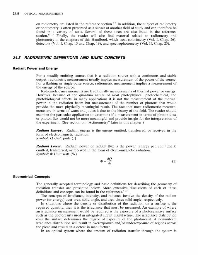
FIGURE 1 The solid angle at the center of the sphere is the surface area enclosed in the base of the cone divided by the square of the sphere radius .
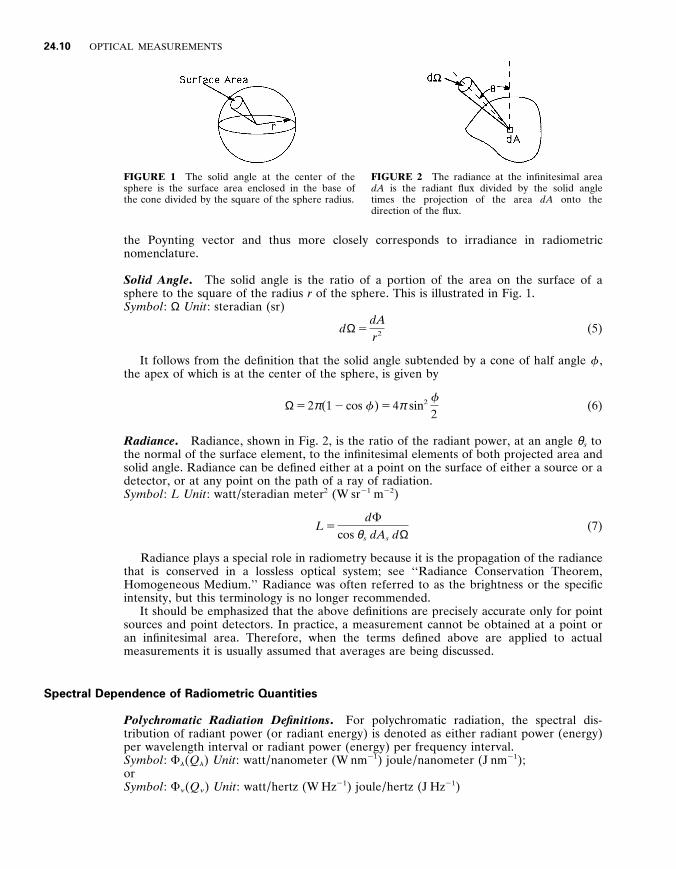
FIGURE 2 The radiance at the infinitesimal area dA is the radiant flux divided by the solid angle times the projection of the area dA onto the direction of the flux .
the Poynting vector and thus more closely corresponds to irradiance in radiometric nomenclature .
Solid Angle . The solid angle is the ratio of a portion of the area on the surface of a sphere to the square of the radius r of the sphere . This is illustrated in Fig . 1 . Symbol : Ω Unit : steradian (sr)
d Ω 5 dA
r 2 (5)
It follows from the definition that the solid angle subtended by a cone of half angle f , the apex of which is at the center of the sphere , is given by
Ω 5 2 π (1 2 cos f ) 5 4 π sin 2 f
2 (6)
Radiance . Radiance , shown in Fig . 2 , is the ratio of the radiant power , at an angle θ s to the normal of the surface element , to the infinitesimal elements of both projected area and solid angle . Radiance can be defined either at a point on the surface of either a source or a detector , or at any point on the path of a ray of radiation . Symbol : L Unit : watt / steradian meter 2 (W sr 2 1 m 2 2 )
L 5 d F
cos θ s dA s d Ω (7)
Radiance plays a special role in radiometry because it is the propagation of the radiance that is conserved in a lossless optical system ; see ‘‘Radiance Conservation Theorem , Homogeneous Medium . ’’ Radiance was often referred to as the brightness or the specific intensity , but this terminology is no longer recommended .
It should be emphasized that the above definitions are precisely accurate only for point sources and point detectors . In practice , a measurement cannot be obtained at a point or an infinitesimal area . Therefore , when the terms defined above are applied to actual measurements it is usually assumed that averages are being discussed .
Spectral Dependence of Radiometric Quantities
Polychromatic Radiation Definitions . For polychromatic radiation , the spectral dis- tribution of radiant power (or radiant energy) is denoted as either radiant power (energy) per wavelength interval or radiant power (energy) per frequency interval . Symbol : F l ( Q l ) Unit : watt / nanometer (W nm 2 1 ) joule / nanometer (J nm 2 1 ) ; or Symbol : F … ( Q … ) Unit : watt / hertz (W Hz 2 1 ) joule / hertz (J Hz 2 1 )

RADIOMETRY AND PHOTOMETRY 24 .11
It follows that F l d l is the radiant power in the wavelength interval l to l 1 d l , and w … d … is the radiant power in the frequency interval … to … 1 d … . The total radiant power over the entire spectrum is therefore
F 5 E
0 F l d l (8 a )
or
F 5 E
0 F … d … (8 b )
Another way of stating the preceding is that monochromatic radiant power F l is the radiant power in an infinitesimal wavelength interval d l .
If l is the wavelength in the medium corresponding to the frequency … , and since … 5 c / n l , where c is the speed of light in a vacuum and n is the index of refraction of the medium , then
d … 5 c
n l 2 d l (9)
and
l F l 5 … F … (10)
Since the wavelength changes with the index of refraction of the medium , it is becoming more common to use the vacuum wavelength , l 5 c / … . It is particularly important in high-accuracy applications to state explicitly whether or not the vacuum wavelength is being used .
Spectral versions of the other radiometric quantities , i . e ., radiant energy , radiance , etc ., are defined similarly .
Polychromatic Radiation Calculations . As an example of the application of the concept of the spectral dependence of a radiometric quantity , consider the calculation of the response of a radiometer consisting of a detector and a spectral filter . The spectral responsivity of a detector R ( l ) is the ratio of the output signal to the radiant input at each wavelength l . The output is usually an electrical signal , such as a photocurrent i , and the input is a radiometric quantity , such as radiant power . The spectral transmittance of a filter τ ( l ) is the ratio of the output radiant quantity to the input radiant quantity at each wavelength l . For a spectral radiant power F l , the photocurrent i of the radiometer is
i 5 E
0 R ( l ) τ ( l ) F l d l (11)
In practice , either the responsivity of the detector or the transmittance of the filter are nonzero only within a limited spectral range . The integral need be evaluated only within the wavelength limits where the integrand is nonzero .
Photometry
The radiation transfer concepts , i . e ., geometrical principles , of photometry are the same as those for radiometry . The exception is that the spectral responsivity of the detector , the human eye , is specifically defined . Photometric quantities are related to radiometric quantities via the spectral ef ficiency functions defined for the photopic and scotopic CIE
24 .12 OPTICAL MEASUREMENTS
Standard Observer . The generally accepted values of the photopic and scotopic human eye response function are represented in the ‘‘Photometry’’ section in Table 2 .
Luminous Flux . The photometric equivalent of radiant power is luminous flux , and the unit that is equivalent to the watt is the lumen . Luminous flux is spectral radiant flux weighted by the appropriate eye response function . The definition of luminous flux for the photopic CIE Standard Observer is Symbol : F y Unit : lumen (lm)
F y 5 K m E F l V ( l ) d l (12)
where V ( l ) is the spectral luminous ef ficiency function and K m is the luminous ef ficacy for photopic vision . The spectral luminous ef ficacy is defined near the maximum , l m 5 555 nm , of the photopic ef ficiency function to be approximately 683 lm W 2 1 .
Definitions of the Density of Luminous Flux . Illuminance . Illuminance is the photometric equivalent of irradiance ; that is , illumin-
ance is the luminous flux per unit area . Symbol : E y Unit : lumen / meter 2 (lm m 2 2 )
E y 5 d F y
cos θ d dA d 5
d F K m E F l V ( l ) d l G cos θ d dA d
(13)
Luminous Intensity Luminous intensity is the photometric equivalent of radiant intensity . Luminous intensity is the luminous flux per solid angle . For historical reasons , the unit of luminous intensity , the candela—not the lumen—is defined as the base unit for photometry . However , the units for luminous intensity can either be presented as candelas or lumens / steradian . Symbol : I y Unit : candela or lumen / steradian (cd or lm sr 2 1 )
I y 5 d w y
d Ω 5
d F K m E F l V ( l ) d l G d Ω
(14)
Luminance . Luminance is the photometric equivalent of radiance . Luminance is the luminous flux per unit area per unit solid angle . Symbol : L y Unit : candela / meter 2 (cd m 2 2 )
L y 5 d F y
cos θ s dA s d Ω 5
d F K m E F l V ( l ) d l G cos θ s dA s d Ω
(15)
Actinometry
Radiant Flux to Photon Flux Con y ersion . Actinometric measurement practice closely follows that of general radiometry except that the quantum nature of light rather than its thermal ef fect is emphasized . In actinometry , the amount of electromagnetic radiation being transferred is measured in units of photons per second (photon flux) . The energy of a single photon is
Q 5 h … (16)
RADIOMETRY AND PHOTOMETRY 24 .13
where … is the frequency of the radiation and h is Planck’s constant , 6 . 6262 3 10 2 3 4 J s . For monochromatic radiant power F l , measured as watts and wavelength l , measured as nanometers , the number of photons per second N l in the monochromatic radiant beam is
N l 5 5 . 0341 3 10 1 5 n l F l (17)
Photon Dose and the Einstein . Dose is the total number of photons impinging on a sample . For a monochromatic beam of radiant power F l that irradiates a sample for a time t seconds , the dose U measured as Einsteins is
U 5 8 . 3593 3 10 2 9 n l F l t (18)
The Einstein is a unit of energy used in photochemistry . An Einstein is the amount of energy in one mole (Avogadro’s number , 6 . 0222 3 10 2 3 ) of photons .
Conversions Between Radiometry , Photometry , and Actinometry
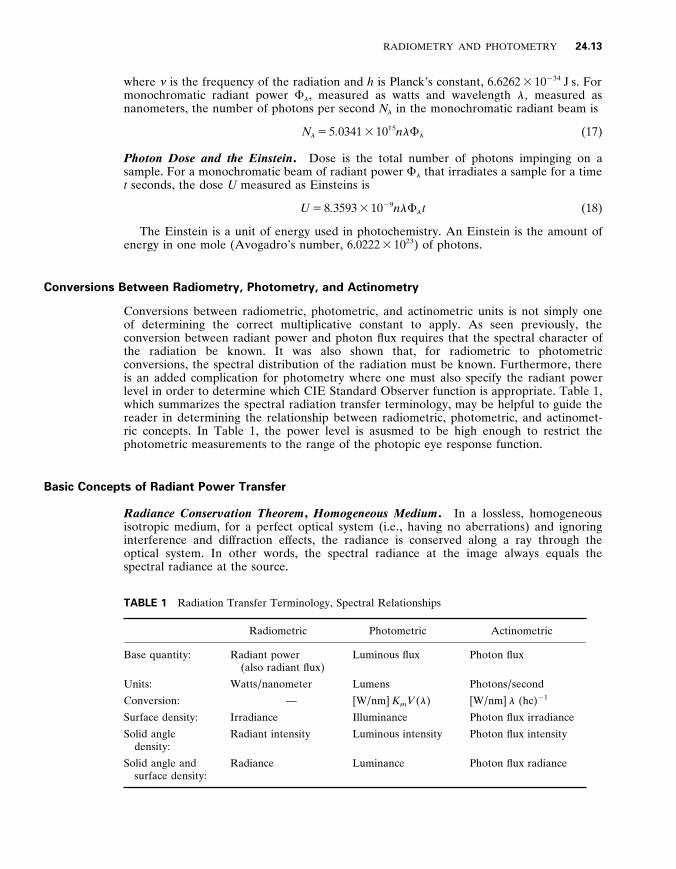
Conversions between radiometric , photometric , and actinometric units is not simply one of determining the correct multiplicative constant to apply . As seen previously , the conversion between radiant power and photon flux requires that the spectral character of the radiation be known . It was also shown that , for radiometric to photometric conversions , the spectral distribution of the radiation must be known . Furthermore , there is an added complication for photometry where one must also specify the radiant power level in order to determine which CIE Standard Observer function is appropriate . Table 1 , which summarizes the spectral radiation transfer terminology , may be helpful to guide the reader in determining the relationship between radiometric , photometric , and actinomet- ric concepts . In Table 1 , the power level is asusmed to be high enough to restrict the photometric measurements to the range of the photopic eye response function .
Basic Concepts of Radiant Power Transfer
Radiance Conser y ation Theorem , Homogeneous Medium . In a lossless , homogeneous isotropic medium , for a perfect optical system (i . e ., having no aberrations) and ignoring interference and dif fraction ef fects , the radiance is conserved along a ray through the optical system . In other words , the spectral radiance at the image always equals the spectral radiance at the source .
TABLE 1 Radiation Transfer Terminology , Spectral Relationships
Radiometric Photometric Actinometric
Base quantity : Radiant power (also radiant flux)
Luminous flux Photon flux
Units : Watts / nanometer Lumens Photons / second
Conversion : — [W / nm] K m V ( l ) [W / nm] l (hc) 2 1
Surface density : Irradiance Illuminance Photon flux irradiance
Solid angle density :
Radiant intensity Luminous intensity Photon flux intensity
Solid angle and surface density :
Radiance Luminance Photon flux radiance
24 .14 OPTICAL MEASUREMENTS
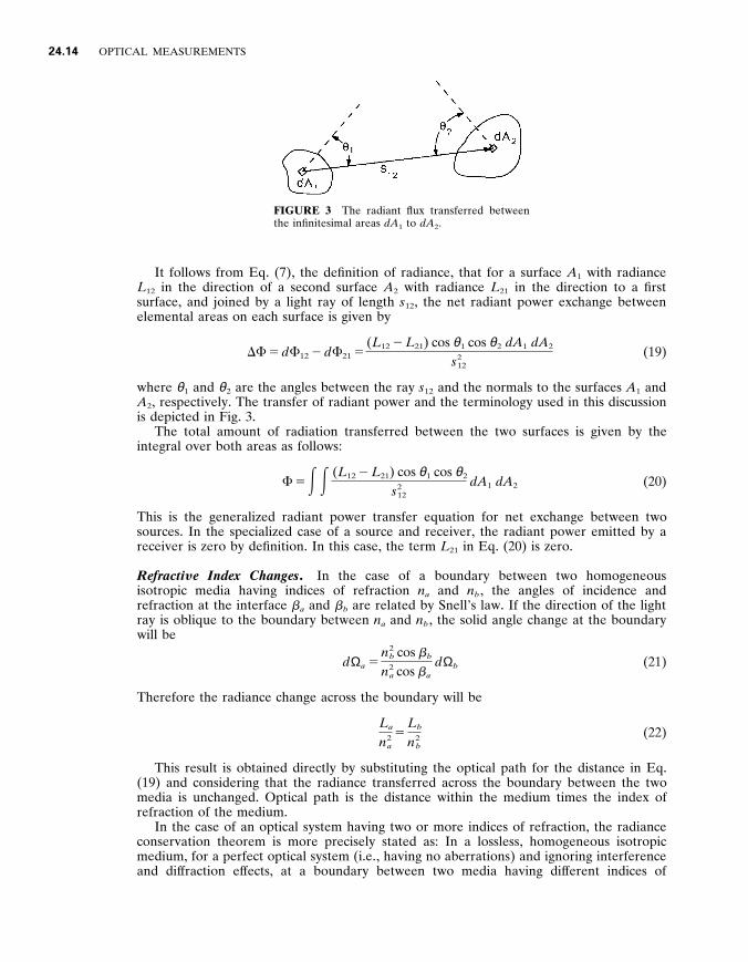
FIGURE 3 The radiant flux transferred between the infinitesimal areas dA 1 to dA 2 .
It follows from Eq . (7) , the definition of radiance , that for a surface A 1 with radiance L 1 2 in the direction of a second surface A 2 with radiance L 2 1 in the direction to a first surface , and joined by a light ray of length s 1 2 , the net radiant power exchange between elemental areas on each surface is given by
DF 5 d F 1 2 2 d F 2 1 5 ( L 1 2 2 L 2 1 ) cos θ 1 cos θ 2 dA 1 dA 2
s 2 12
(19)
where θ 1 and θ 2 are the angles between the ray s 1 2 and the normals to the surfaces A 1 and A 2 , respectively . The transfer of radiant power and the terminology used in this discussion is depicted in Fig . 3 .
The total amount of radiation transferred between the two surfaces is given by the integral over both areas as follows :
F 5 E E ( L 1 2 2 L 2 1 ) cos θ 1 cos θ 2
s 2 12
dA 1 dA 2 (20)
This is the generalized radiant power transfer equation for net exchange between two sources . In the specialized case of a source and receiver , the radiant power emitted by a receiver is zero by definition . In this case , the term L 2 1 in Eq . (20) is zero .
Refracti y e Index Changes . In the case of a boundary between two homogeneous isotropic media having indices of refraction n a and n b , the angles of incidence and refraction at the interface b a and b b are related by Snell’s law . If the direction of the light ray is oblique to the boundary between n a and n b , the solid angle change at the boundary will be
d Ω a 5 n 2
b cos b b
n 2 a cos b a
d Ω b (21)
Therefore the radiance change across the boundary will be
L a
n 2 a
5 L b
n 2 b
(22)
This result is obtained directly by substituting the optical path for the distance in Eq . (19) and considering that the radiance transferred across the boundary between the two media is unchanged . Optical path is the distance within the medium times the index of refraction of the medium .
In the case of an optical system having two or more indices of refraction , the radiance conservation theorem is more precisely stated as : In a lossless , homogeneous isotropic medium , for a perfect optical system (i . e ., having no aberrations) and ignoring interference and dif fraction ef fects , at a boundary between two media having dif ferent indices of
RADIOMETRY AND PHOTOMETRY 24 .15
refraction the radiance divided by the square of the refractive index is conserved along a ray through the optical system .
Radiati y e Transfer Through Absorbing Media . For radiation transmitted through an absorbing and / or scattering medium , the radiance is not conserved . This is not only because of the loss due to the absorption and / or scattering but the medium could also emit radiation . The emitted light will be due to thermal emission (see the discussion on blackbody radiation later in this chapter) . In some cases , the medium may also be fluorescent . Fluorescence is the absorption of radiant energy at one wavelength with subsequent emission at a dif ferent wavelength .
Historically , the study of radiative transfer through absorbing and / or scattering media dealt with the properties of stellar atmospheres . Presently , there is considerable interest in radiative transfer measurements of the earth and its atmosphere using instruments on board satellites or aircraft . An accurate measure of the amount of reflected sunlight (approximately 400 to 2500 nm) or the thermally emitted infrared (wavelengths . 2500 nm) requires correction for the absorption , scattering , and , in the infrared , the emission of radiation by the atmosphere . This specialized topic will not be considered here . Detailed discussion is available in the references . 1 4 – 1 6
2 4 . 4 RADIANT TRANSFER APPROXIMATIONS
The solution to the generalized radiant power transfer equation is typically quite complex . However , there are several useful approximations that in some instances can be employed to obtain an estimate of the solution of Eq . (20) . We shall consider the simpler case of a source and a detector rather then the net radiant power exchange between two sources , since this is the situation commonly encountered in an optical system . In this case , Eq . (20) becomes
F 5 E E L cos θ s cos θ d
s 2 sd
dA s dA d (23)
where the subscripts s and d denote the source and detector , respectively . Here it is assumed the detector behaves as if it were a simple aperture . That is , it responds equally to radiation at any point across its surface and from any direction . Such a detector is often referred to as a cosine corrected detector . Of course , deviations from ideal detection behavior within the spatial and angular range of the calculation reduces the accuracy of the calculation .
Point-to-point Approximation : Inverse Square Law
The simplest approximations are obtained by assuming radiant flux transfer between a point source emitting uniformly in all directions and a point detector . The inverse square law is an approximation that follows directly from the definitions of intensity , solid angle , and irradiance , Eqs . (2) , (4) , and (5) , respectively . The irradiance (at an infinitesimal area whose normal is along the direction of the light ray) times the square of the distance from a point source equals the intensity of the source
I 5 F
A s 2 5 Es 2 (24)
24 .16 OPTICAL MEASUREMENTS
The relationship between the uniformly emitted radiance and the intensity of a point source is obtained similarly from Eqs . (4) and (7) :
L 5 I
A s (25)
These point-to-point relationships are perhaps most important as a test of the accuracy of a radiation transfer calculation at the limit as the areas approach zero .
Lambertian Approximation : Uniformly Radiant Areas
Lambertian Sources . A very useful concept for the approximation of radiant power transfer is that of a source having a radiance that is uniform across its surface and uniformly emits in all directions from its surface . Such a uniform source is commonly referred to as a lambertian source .
For the case of a lambertian source , Eq . (23) becomes
F 5 L E E cos θ s cos θ d
s 2 sd
dA s dA d (26)
Configuration Factor . The double integral in Eq . (26) has been given a number of dif ferent names : configuration factor , radiation interaction factor , and projected solid angle . There is no generally accepted terminology for this concept , although configuration factor appears most frequently . Analytical solutions to the double integral have been found for a variety of dif ferent shapes of source and receiver . Tabulations of these exact solutions to the integral in Eq . (26) are usually found in texts on thermal engineering , 1 7 – 1 8
under the heading of radiant heat transfer or configuration factor . Radiation transfer between complex shapes can often be determined by using various
combinations of configuration factors . This technique is often referred to as configuration factor algebra . 1 7 The surfaces are treated as pieces , each with a calculable configuration factor , and the separate configuration factors are combined to obtain the ef fective configuration factor for the complete surface .
E tendue . The double integral in Eq . (26) is often used as a means to characterize the flux-transmitting capability of an optical system in a way that is taken to be independent of the radiant properties of the source . Here the double integral is written as being over area and solid angle :
F 5 L E E cos θ d dA s d Ω (27)
In this case , the surface of the lambertian source is assumed perpendicular to the optic axis and to lie in the entrance window of the optical system . The solid angle is measured from a point on the source to the entrance pupil . The e tendue E of an optical system of refractive index n is defined as
E 5 n 2 E E cos θ d dA s d Ω (28)
Equation (28) is sometimes referred to as the throughput of an optical system . Total Flux into a Hemisphere . The total amount of radiation emitted from a
lambertian source of area dA s into the hemisphere centered at dA s (or received by a hemispherical , uniform detector centered at dA s ) is obtained from integrating Eq . (26) over the area A d . Note that the ray s s d is everywhere normal to the surface of the hemisphere ; i . e ., cos θ d 5 1 .
F 5 L π E dA s (29)

RADIOMETRY AND PHOTOMETRY 24 .17
Using Eq . (3) , the definition of the exitance , the radiance at each point on the surface of the source is
L 5 M π
(30)
Because of the relationship expressed in Eq . (30) , Eq . (26) is often written in terms of the exitance .
F 5 M π E E cos θ s cos θ d
s 2 sd
dA s dA d (31)
In this case , the factor π is considered to be part of the configuration factor . Note again that there is no generally accepted definition of the configuration factor .
Radiation Transfer Between a Circular Source and Detector . The particular case of radiation transfer between circular apertures , the centers of which are located along the same optical axis as shown in Fig . 4 , is a configuration common to many optical systems and is therefore illustrated here . The radius of the source (or first aperture) is r s , the detector (second aperture) radius is r d , and the distance between the centers is s s d . The exact solution of the integral in Eq . (26) yields
F 5 2 L ( π r s r d ) 2
r 2 s 1 r 2
d 1 s 2 sd 1 [( r 2
s 1 r 2 d 1 s 2
sd ) 2 2 4 r 2 s r
2 d ] 1 / 2 (32)
This result can be approximated for the case where the sum of the squares of the distance and radii is large compared to the product of the radii , that is , ( r 2
s 1 r 2 d 1 s 2
sd ) 2 r s r d , so that Eq . (32) reduces to
F > L ( π r s r d ) 2
r 2 s 1 r 2
d 1 s 2 sd
(33)
From this expression the irradiance at the detector can be obtained
E 5 F
A d >
LA s
r 2 s 1 r 2
d 1 s 2 sd
> LA s
s 2 sd
(34)
where A s is the area of the lambertian disk and A d is the detector area . The approximation at the extreme right is obtained by assuming that the radii are completely negligible with respect to the distance . This is the same result that would be obtained from a point-to-point approximation .
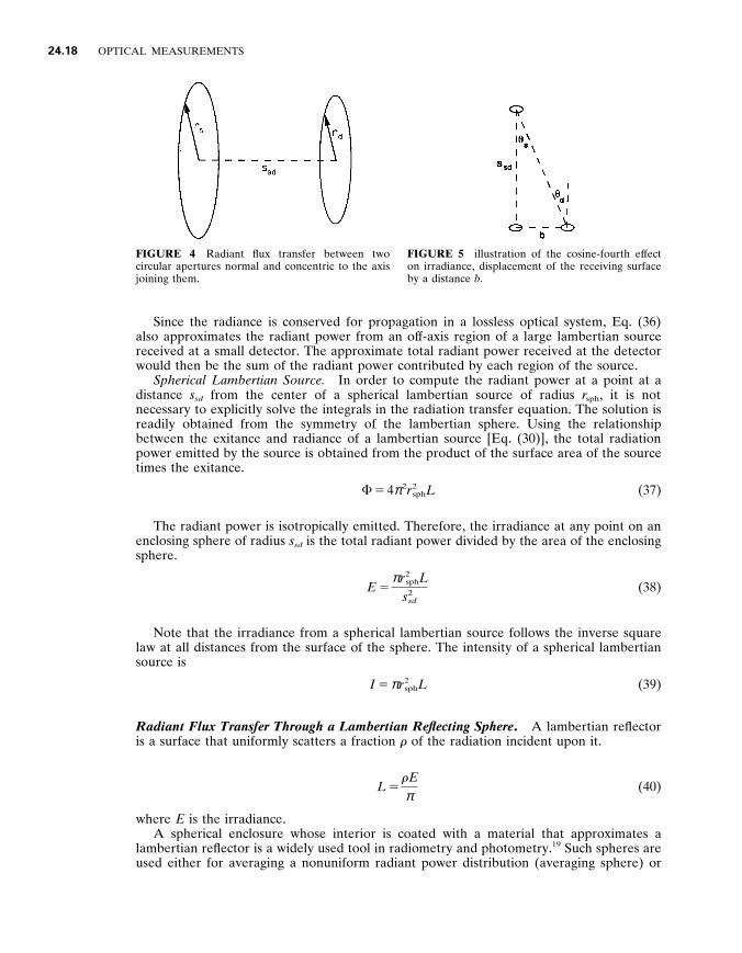
Of f - axis Irradiance : Cosine - to - the - Fourth Approximation . Equation (34) describes the irradiance from a small lambertian disk to a detector on the ray axis and where both surfaces are perpendicular to the ray . If the detector is moved of f-axis by a distance b as depicted in Fig . 5 , the ray from A s to A d will then be at an angle with respect to the normal at both surfaces as follows
θ s 5 θ d 5 θ 5 tan 2 1 S b s s d D (35)
The projected areas are then ( A s cos θ ) and ( A d cos θ ) . In addition , the distance from the source to the detector increases by the factor (1 / cos θ ) . The radiant power at a distance b away from the axis therefore decreases by the fourth power of the cosine of the angle formed between the normal to the surface and the ray .
F > LA s A d
s 2 sd
cos 4 θ (36)
24 .18 OPTICAL MEASUREMENTS
FIGURE 4 Radiant flux transfer between two circular apertures normal and concentric to the axis joining them .
FIGURE 5 illustration of the cosine-fourth ef fect on irradiance , displacement of the receiving surface by a distance b .
Since the radiance is conserved for propagation in a lossless optical system , Eq . (36) also approximates the radiant power from an of f-axis region of a large lambertian source received at a small detector . The approximate total radiant power received at the detector would then be the sum of the radiant power contributed by each region of the source .
Spherical Lambertian Source . In order to compute the radiant power at a point at a distance s s d from the center of a spherical lambertian source of radius r s p h , it is not necessary to explicitly solve the integrals in the radiation transfer equation . The solution is readily obtained from the symmetry of the lambertian sphere . Using the relationship between the exitance and radiance of a lambertian source [Eq . (30)] , the total radiation power emitted by the source is obtained from the product of the surface area of the source times the exitance .
F 5 4 π 2 r 2 sph L (37)
The radiant power is isotropically emitted . Therefore , the irradiance at any point on an enclosing sphere of radius s s d is the total radiant power divided by the area of the enclosing sphere .
E 5 π r 2
sph L s 2
sd
(38)
Note that the irradiance from a spherical lambertian source follows the inverse square law at all distances from the surface of the sphere . The intensity of a spherical lambertian source is
I 5 π r 2 sph L (39)
Radiant Flux Transfer Through a Lambertian Reflecting Sphere . A lambertian reflector is a surface that uniformly scatters a fraction r of the radiation incident upon it .
L 5 r E π
(40)
where E is the irradiance . A spherical enclosure whose interior is coated with a material that approximates a
lambertian reflector is a widely used tool in radiometry and photometry . 1 9 Such spheres are used either for averaging a nonuniform radiant power distribution (averaging sphere) or
RADIOMETRY AND PHOTOMETRY 24 .19
for measuring the total amount of radiant power emitted from a source (integrating sphere) .
The sphere has the useful property whereby the solid angle subtended by any one section of the wall times the projected area is constant over all other points on the inside surface of the sphere . Therefore , if radiation falling on any point within the sphere is uniformly reflected , the reflected radiation will be uniformly distributed , i . e ., produce uniform irradiance , throughout the interior . This result follows directly from the symmetry of the sphere .
Consider a sphere of radius r s p h and the radiant power transfer between two points on the inner surface . The normals to the two points are radii of the sphere and form an isosceles triangle when taken with the ray joining the points . Therefore , the angles between the ray and the normals to each point are equal . From Eq . (26)
F 5 L E E cos 2 θ s 2
sd
dA s dA d (41)
The length of the ray joining the points is 2 r s p h cos θ . The irradiance is therefore
E 5 F
A d 5
LA s
4 r 2 sph
(42)
which is independent of the angle θ . If F i n is the radiant power entering the sphere , the irradiance at any point on the sphere after a single reflection will be
E 5 r F i n
4 π r 2 sph
(43)
A fraction r of the flux will be reflected and again uniformly distributed over the sphere . After multiple reflections the irradiance at any point on the wall of the sphere is
E 5 ( r 1 r 2 1 r 3 1 ? ? ? ) F i n
4 π r 2 sph
5 r F i n
(1 2 r ) A s p h (44)
where A s p h is the surface area of the sphere . The flux F o u t exiting the sphere through a port of area A o u t is
F o u t 5 r F i n A o u t
(1 2 r ) A s p h (45)
In Eq . (45) it is assumed that the loss of radiation at the entrance and exit ports is negligible and does not af fect the symmetry of the radiation distribution .
The ef fect of the radiation lost through the entrance and exit ports is approximated as follows . After the first reflection , the fraction of radiation lost in each subsequent reflection is equal to the combined areas of the ports divided by the sphere area .
g 5 A i n 1 A o u t
A s p h (46)
Using this in Eq . (44) yields
F o u t 5 r F i n A o u t
(1 2 r g ) A s p h (47)
Since the sphere is approximately a lambertian source , the radiance at the exit port is
L 5 r F i n
(1 2 r g ) π A s p h (48)
24 .20 OPTICAL MEASUREMENTS
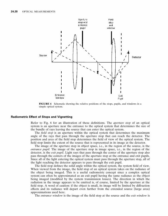
FIGURE 6 Schematic showing the relative positions of the stops , pupils , and windows in a simple optical system .
Radiometric Ef fect of Stops and Vignetting
Refer to Fig . 6 for an illustration of these definitions . The aperture stop of an optical system is an aperture near the entrance to the optical system that determines the size of the bundle of rays leaving the source that can enter the optical system .
The field stop is an aperture within the optical system that determines the maximum angle of the rays that pass through the aperture stop that can reach the detector . The position and area of the field stop determines the field of view of the optical system . The field stop limits the extent of the source that is represented in its image at the detector .
The image of the aperture stop in object space , i . e ., in the region of the source , is the entrance pupil . The image of the aperture stop in image space , i . e ., in the region of the detector , is the exit pupil . Light rays that pass through the center of the aperture stop also pass through the centers of the images of the aperture stop at the entrance and exit pupils . Since all of the light entering the optical system must pass through the aperture stop , all of the light reaching the detector appears to pass through the exit pupil .
The field stop defines the solid angle within the optical system , the system field of view . When viewed from the image , the field stop of an optical system takes on the radiance of the object being imaged . This is a useful radiometric concept since a complex optical system can often be approximated as an exit pupil having the same radiance as the object being imaged (modified by the system transmission losses) . The direction in which the radiation in the image appears to be emitted is , of course , limited by the aperture at the field stop . A word of caution : if the object is small , its image will be limited by dif fraction ef fects and its radiance will depart even further from the extended source (large area) approximations used here .
The entrance window is the image of the field stop at the source and the exit window is
RADIOMETRY AND PHOTOMETRY 24 .21
the image of the field stop at the detector . If the field stop coincides with the detector , i . e ., the detector is in the image plane of the optical system , then the entrance window will correspond with the object plane on the source . If the field stop does not coincide with the image plane at the detector , then because of parallax , dif ferent portions of the source will be visible from dif ferent points within the exit pupil . This condition , known as y ignetting , causes a decrease in the irradiance at the of f-axis points on the detector or image plane .
Approximate Radiance at an Image
Aplanatic Optical Systems . Except for rays that lie on the optic axis , the radiance of an image must be based on a knowledge of the image quality since any aberrations introduced by the optical system divert some of the of f-axis rays away from the image .
Consider a well-corrected optical system that is assumed to be aplanatic for the source and image points . That is , the optical system obeys Abbe’s sine condition which is
n s h s sin θ s 5 n d h d sin θ d (49)
where n s and n d are the refractive indices of the object (source) and image (detector) spaces , h s and h d are the object and image heights , and θ s and θ d are the angles between the of f-axis rays and the optic axis in object and image space . From Eq . (27) the flux radiated by a small lambertian source of area A s into the solid angle of the optical system is
F > 2 π LA s E θ s
0 cos θ sin θ d θ 5 π LA s sin 2 θ s (50)
The dif ferential of the solid angle is obtained from Eq . (6) . Since F is the radiant flux at the image and A d is the area of the image , the irradiance at the image is
E 5 F
A d 5
π LA s
A d sin 2 θ s (51)
If h s and h d are the radii of circular elements A s and A d , then according to Abbe’s sine condition
A s
A d 5
n 2 d sin 2 θ d
n 2 s sin 2 θ s
(52)
The irradiance at the image is
E 5 π Ln 2
d
n 2 s
sin 2 θ d (53)
Numerical Aperture and F - number . The quantity n d sin θ d in Eq . (53) is called the numerical aperture of the imaging system . The irradiance of the image is proportional to the square of the numerical aperture . Geometrically speaking , the image irradiance increases with the angle of the cone of light converging on the image .
Another approximate measure of the image irradiance of an optical system is the F-number , f 4 (sometimes called the focal ratio) defined by the ratio of focal length (in the image space) f to the diameter D of the entrance pupil . For a source at a very large distance
f 4 5 f
D 5
1 2 tan θ d
> 1
2 sin θ d (54)
The approximate image irradiance expressed in terms of the F-number is
E > π L S n d
2 n s f 4 D 2
(55)
24 .22 OPTICAL MEASUREMENTS
2 4 . 5 ABSOLUTE MEASUREMENTS
An absolute measurement , often referred to as an absolute calibration , is a measurement that is based upon , i . e ., derived from , one of the internationally recognized units of physical measurement . These units are known as the SI units (Syste me International d’Unite s 2 0 ) . The absolute SI base units are the meter , second , kilogram , kelvin , ampere , candela , and mole . The definitions of the SI units , the methods for their realization , or their physical embodiment are a matter of international agreement under the terms of the 1875 Treaty of the Meter . A convenient method (but often not a suf ficient condition) for achieving absolute accuracy is to obtain traceability to one of the SI units via a calibration transfer standard issued by one of the national standards laboratories . The United States standards laboratory is the National Institute of Standards and Technology (NIST , formerly the National Bureau of Standards) .
A relative measurement is one that is not required to be traceable to one of the SI units . Relative measurements are usually obtained as the ratio of two measurements . An example of a relative measurement is the determination of the transmittance of an optical material wherein the ratio of the output radiant power to the input radiant power is measured ; the measurement result is independent of SI units .
Absolute Accuracy and Traceability
Establishment of legal traceability to an SI unit requires that one obtain legally correct documentation , i . e ., certification , of the device that serves as the calibration transfer standard and sometimes of the particular measurement process in which the device is to be used . Certification of legal traceability within each nation is obtained from the national standards laboratory of that nation . Often another nation’s standards laboratory can be used to establish legal traceability , provided that there exists the legal framework for mutual recognition of the legality of each other’s standards .
In order to establish accurate traceability to an SI unit , one needs to determine the total accumulated error arising from : (1) the realization of the base SI unit ; (2) if applicable , the derivation of an associated measurement quantity ; (3) if applicable , scaling to a higher or lower value ; and (4 , 5 ? ? ? ) transfer of the calibration from one device to another . The last entries must include the instability of the calibration transfer devices ; the others may or may not involve a transfer device .
Legal traceability to SI units does not guarantee accurate traceability and vice versa . In order to obtain accurate traceability , it is not necessary to prove traceability to a national standards laboratory . Instead , the measurement must trace back to one of the SI units . However , it is usually convenient to establish accurate traceability via one of the national standards laboratories . The degree of convenience and accuracy will depend upon the accuracy of the measurement method and type of calibration transfer device available from the particular national standards laboratory .
As an example of an absolute radiometric measurement chain consider the following method for determining absolute spectral irradiance (based on the method used by NIST 2 1 ) . The steps that lead to the calibration of a spectral irradiance meter are : (1) determination of the absolute temperature of a simulated planckian radiator (i . e ., a blackbody ; see later discussion) ; (2) derivation of the spectral radiance output of the blackbody simulator (by evaluation of the deviations from the ideal radiator , i . e ., deviations from Planck’s law) ; (3) scaling up to the radiance level produced by an incandescent lamp ; (4) transfer of spectral radiance from the blackbody simulator to the incandescent lamp ; (5) derivation of spectral irradiance from radiance via the measure- ment of solid angle ; (6) transfer of spectral irradiance to another type of incandescent lamp ; (7) spectral irradiance transfer from primary standard lamps to secondary standard
RADIOMETRY AND PHOTOMETRY 24 .23
lamps ; (8 , 9 ? ? ? x -1) other lamp-to-lamp transfers (to get to the user laboratory) ; and ( x ) calibration of the response of the spectral irradiance meter via the final calibration transfer lamp . The absolute accuracy of the spectral irradiance meter is established by evaluating and summing the errors accumulated in all the measurements listed . Measurements 1 through 7 are performed at NIST and NIST estimates the accuracy of their traceability to the SI temperature unit . Note that it is up to the user to determine the accuracy of the remaining x -7 measurements . The major uncertainty is typically the instability (noise and drift) of the incandescent lamps used at several steps . Lamp drift is often not quantifiable .
Other methods for the determination of absolute spectral irradiance exist , 22–24 and some are employed by other national standards laboratories . Each method has a unique set of errors associated with it . A comparison of the absolute measurements obtained via independent methods is the best means of verifying absolute accuracy . If the comparison shows that the two calibrations agree to within their combined uncertainty , then the hypothesis that the calibration and the true value are the same within the uncertainty estimation is strengthened . Comparison of independent methods of calibration provides the best available verification of absolute accuracy . However , a note of caution is in order because compensating mistakes can occur and , even in the case of good agreement between independent methods , there is no 100 percent guarantee of accurate traceability .
Relative measurements do not require traceability to one of the SI base units . Since a relative measurement is the ratio of two measurements , accuracy is assured by the linearity of the measuring instrument (or by a precise knowledge of its nonlinearity function) and by the elimination of dif ferences (or a knowledge of the ef fect of such dif ferences) in the two measurements being ratioed . For relative measurements the best available assurance of accuracy is also obtained by comparison to a measurement obtained by an independent method .
Types of Errors , Uncertainty Estimates , and Error Propagation
It is almost pointless to state a value for an absolute or relative measurement without an estimate of the uncertainty and the degree of confidence to be placed in the uncertainty estimate . Verification of the accuracy and the confidence limits is not only desirable but is often a legal requirement .
The accuracy and the uncertainty of a measurement are synonymous . The usual terminology is that a measurement is ‘‘accurate to within Ú x ’’ or ‘‘uncertain to within Ú x ’’ , where x is either a fraction (percent) of the measured value or an interval within which the true value is known to within some degree of confidence . The degree of confidence in the uncertainty estimate is the confidence interval or s -level .
Errors are classified as type A errors , also known as random errors , and type B , or systematic errors . Type A errors are the variations due to the ef fects of uncontrolled variables . The magnitude of these ef fects is usually small and successive measurements form a random sequence . Type B errors are not detectable as variations since they do not change for successive measurements with a given apparatus and measurement method . Type B errors arise because of dif ferences between the ideal behavior embodied in fundamental laws of physics and real behavior embodied in an experimental simulation of the ideal . A type B error could also be a function of the quantity being measured ; for example , in a blackbody radiance standard using the freezing point of a metal and its defined temperature instead of the true absolute temperature .
Type A errors are estimated using standard statistical methods . If the distribution of the measurements is known (e . g ., either Gaussian , which is often called a normal distribution , or Poisson) , then one uses the formalism appropriate to the distribution . Unless enough data is obtained to establish that the distribution is not Guassian , it is usual to assume a gaussian distribution . A brief discussion of Gaussian statistical concepts and terminology is given here to guide the reader in interpreting or determining the uncertainty in a
24 .24 OPTICAL MEASUREMENTS
radiometric or photometric calibration . One of the many texts on statistics , 2 5 – 2 6 or experimental methods , 2 7 should be consulted for a more thorough discussion .
The mean value m , the standard deviation s , and the standard deviation of the mean s m , of a set of measurements x i , are estimated for a small sample from a gaussian distribution of measurements as follows :
m 5 O i
x i
h (56)
s 2 5 O ( x i 2 m ) 2
h 2 1 (57)
s m 5 s
4 h (58)
where i 5 1 to h , and h is the total number of measurements . The standard deviation is an estimate of the spread of the individual measurements
within a sample , and it approaches a constant value as h is increased . The standard deviation of the mean is an estimate of the spread of the values of the
mean that would be obtained from several dif ferent sets of sample measurements . The standard deviation of the mean decreases as the number of samples in a set increases , since the estimate of the mean approaches the true mean for an infinite data set . The standard deviation of the mean is used in the estimate of the confidence interval assigned to the reported value of the mean .
The degree of confidence to which a reported value of the mean is valid is known as the confidence inter y al (CI) . If it is assumed that a very large set of measurements has been sampled , then the CI is often given in terms of the number of standard deviations of the mean (one- s level , two- s level , etc . ) within which the type A error of a reported value is known .
The CI is the probability that the mean from a normal distribution will be within the estimated uncertainty . That is , for a z -percent confidence interval , z -percent of the measurements will fall inside and (100 2 z ) percent will fall outside of the uncertainty estimate . For small measurement samples from a gaussian distribution , Student’s t-distribution is used to estimate the CI . Tables of Student’s t-distribution along with discussions concerning its use are presented in most statistics textbooks . For large sets of measurements , a one- s level corresponds approximately to a 68-percent CI , a two- s level to a 95-percent CI , and a three- s level to a 99 . 7-percent CI .
The reader is cautioned about using the s level designation to describe the CI for a small sample of measurements . As an example of the small versus large sample dif ference , consider two data sets , one consisting of three samples and the other ten . Using a Student’s t-distribution to estimate the CI for the three sample set , the one- s , two- s , and three- s levels correspond to CIs of 61 percent , 86 percent , and 94 percent , respectively . For the ten-sample set , the respective CIs are 66 percent , 93 percent , and 99 percent . It can be quite misleading to state only the s level of the uncertainty estimate without an indication of the size of the measurement set from which it was drawn . In order to avoid misleading accuracy statements , it is recommended that , instead of simply reporting the s level , either the estimated CI be reported or the standard deviation of the mean be reported along with the number of measurement samples obtained .
Type B error estimates are either educated guesses of the magnitude of the dif ference between the real and the ideal or they are the result of an auxiliary measurement . If an appropriate auxiliary experiment can be devised to measure a systematic or type B error , then it need no longer be considered an error . The result obtained from the auxiliary measurement can usually be used as a correction factor . If a correction factor is applied ,
RADIOMETRY AND PHOTOMETRY 24 .25
then the uncertainty is reduced to the uncertainty associated with the auxiliary experiment .
Most of the ef fort in high-accuracy radiometry and photometry is devoted to reducing type B errors . The first rule for reducing type B errors is to insure that the experiment closely simulates the ideal . The second rule is that the dif ferences between real and ideal should be investigated and that a correction be applied . Unlike type A errors for which an objective theory exists , the educated guess for a type B error is often subjective . For type B errors , neither a confidence interval nor a s level is objectively quantifiable .
Error propagation , error accumulation , or a combined uncertainty analysis is the summation of all the type A and type B uncertainties that contribute to the final measurement in the chain . Because type A errors are truly random , they are uncorrelated and the accumulated type A error is obtained from the square-root of the sum of the squares (also known as root-sum-square , RSS) of the several type A error estimates . Type B uncertainties , however , may be either correlated or uncorrelated . If they are uncorre- lated , the total uncertainty is the RSS of the several estimates . Type B uncertainties that are correlated must be arithmetically summed in a way that accounts for their correlation . Therefore , it is usually desirable to partition type B uncertainties so that they are uncorrelated .
Absolute Sources
Planckian or Blackbody Radiator . A blackbody , or planckian , radiator is a thermal radiation source with a predictable absolute radiance output . An ideal blackbody is a uniform , i . e ., lambertian , source of radiant power having a predictable distribution over area , solid angle , and wavelength . It is used as a standard radiance source from which the other radiometric quantities , e . g ., irradiance , intensity , etc ., can be derived .
Blackbody simulators are in widespread use not only at national standards laboratories but also in many other industrial , academic , and government laboratories . Blackbody simulators are commercially available from a number of manufacturers and cover a wide range of temperatures and levels of accuracy . Because they are in such widespread use as absolute standard sources for a variety of radiometric applications , particularly in the infrared , they are discussed here in some detail . Furthermore , since many practical sources of radiation can be approximated as a thermal radiation source , a blackbody function is often used in developing the radiometric model of an optical system .
An ideal blackbody is a completely enclosed volume containing a radiation field which is in thermal equilibrium with the isothermal walls of the enclosure that is at a known absolute temperature . The radiation in equilibrium with the walls does not depend upon the shape or constitution of the walls provided that the cavity dimensions are much larger than the wavelengths involved in the spectrum of the radiation .
Since the radiometric properties of a blackbody source are completely determined by its temperature , the SI base unit traceability for blackbody-based radiometry is to the kelvin .
Since the radiation field and the walls are in equilibrium , the energy in the radiation field is determined by the temperature of the walls . The relationship between the absolute temperature T and the spectral radiance L l is given by Planck’s law :
L l 5 2 hc 2
n 2 l 5 [ e ( hc / n l kT ) 2 1] 2 1 (59)
Here h is Planck’s constant , c is the speed of light in a vacuum , k is Boltzmann’s constant , l is the wavelength , and n is the index of refraction of the medium . Incorporating the values of the constants in this equation yields ,
24 .26 OPTICAL MEASUREMENTS
Spectral radiance units : W m 2 2 sr 2 1 m m 2 1
L l 5 1 . 1910 3 10 8
n 2 l 5 [ e (1 . 4388 3 10 4 / n l T ) 2 1] 2 1 (60)
It follows that the peak of the spectrum of a blackbody is determined by its temperature (Wein displacement law) .
n l m a x T 5 2898 m m K (61)
It is often useful to measure blackbody spectral radiance in units of photons per second N l . The form of Planck’s law in this case is Spectral radiance units : photons s 2 1 m 2 2 sr 2 1 m m 2 1
N l 5 2 c
n l 4 [ e ( hc / n l kT ) 2 1] 2 1 (62)
The peak of this curve is not at the same wavelength as in the case of radiance measured in units of power . Wein’s displacement law for blackbody radiance measured in photons per second is
n l m a x T 5 3670 m m K (63)
In other applications , the spectral distribution of the blackbody radiation may be required in units of photons per second per frequency interval (symbol : N … ) . This form of Planck’s law is Spectral radiance units : photons s 2 1 m 2 2 sr 2 1 Hz 2 1
N … 5 2 n 2 … 2
c 2 [ e ( h … / kT ) 2 1] 2 1 (64)
and that of Wein’s displacement law is
T
… m a x 5 1 . 701 3 10 2 1 1 K Hz 2 1 (65)
Planck’s law integrated over all wavelengths (or frequencies) leads to the Stefan- Boltzmann law which describes the temperature dependence of the total radiance of a blackbody . For blackbody radiance measured as radiant power , the Stefan-Boltzmann law is Radiance units : W m 2 2 sr 2 1
L 5 1 . 8047 3 10 2 8 n 2 T 4 (66)
Equation (66) is the usual form of the Stefan-Boltzmann law ; however , it can also be derived for blackbody radiance measured as photon flux . Radiance units : photons s 2 1 m 2 2 sr 2 1
N 5 4 . 8390 3 10 1 4 n 2 T 3 (67)
The preceding expressions are valid provided that the cavity dimensions are much larger than the wavelengths involved in the spectrum of the radiation . The restriction imposed by the cavity dimension may lead to significant errors in very high accuracy radiometry or very long wavelength radiometry . For example , in a cube 1 mm on a side and at a wavelength of 1 m m , the approximate correction to Planck’s equation is only 3 3 10 2 7 ; however , if the measurement is made within a 1-nm bandwidth or less , the root mean square fluctuation of the signal is about 2 3 10 2 3 which may not be negligible .
RADIOMETRY AND PHOTOMETRY 24 .27
Recent work describes how well the Planck and Stefan-Boltzmann equations describe the radiation in small cavities and at long wavelengths . 2 8 – 3 0
Blackbody Simulators . An ideal blackbody , being completely enclosed , does not radiate into its surrounds and therefore cannot serve as an absolute radiometric source . A blackbody simulator is a device that does emit radiation but only approximates the conditions under which Planck’s law is valid . In general , a blackbody simulator is an enclosure at some fixed temperature with a hole in it through which some of the radiation is emitted . Some low-accuracy blackbody simulators are fabricated as a flat surface held at a fixed temperature .
A blackbody simulator can be used as an absolute source provided that the type B errors introduced by the deviations from the ideal Planck’s-law conditions are evaluated and the appropriate corrections are applied . In a blackbody simulator there are three sources of type B error : inaccurate surface temperature , nonequilibrium between the radiant surface and the radiation field due to openings in the enclosure , and nonuniformity in the temperature of the radiant surface .
Calculation of the ef fect of a temperature error on the spectral radiance is obtained from the derivative of Planck’s law with respect to temperature .
dL l
L l
5 hc
n l kT [1 2 e 2 ( hc / n l kT ) ] 2 1 dT
T (68)
Since the radiation field is in equilibrium with the surface of the cavity , it is the absolute temperature of the surface that must be measured . It is usually impractical to have the thermometer located on the emitting surface and it is the temperature within the wall that is measured . The dif ference between the temperature within the wall and the surface must therefore be measured , or calculated from a thermal model , and the correction applied .
The error due to nonequilibrium occurs because a practical radiation source cannot be a completely closed cavity . The correction factor for the ef fect on the radiance due to the escaped radiation is obtained from application of Kirchhof f’s law . Simply stated , Kirchhof f’s law states that the absorptive power of a material is equal to its emissive power . According to the principle of detailing balancing , for a body to be in equilibrium in a radiation field , the absorption of radiation by a given element of the surface for a particular wavelength , state of polarization , and in a particular direction and solid angle must equal the emission of that same radiation . If this were not true , the body would either emit more than it absorbs or vice versa , it would not be in equilibrium with the radiation , and it would either heat up or cool of f .
Radiation impinging upon a body is either reflected , transmitted , or absorbed . The fraction of the incident radiation that is reflected r (reflectance) , plus the fraction absorbed a (absorptance) , plus the fraction transmitted τ (transmittance) , is equal to one .
1 5 r 1 a 1 τ (69)
From Kirchhof f’s law for a surface in radiative equilibrium , the fraction of absorbed radiation equals the fraction emitted » (emittance or emissivity) . Therefore , the sum of the reflectance , transmittance , and emittance must also be equal to one . If the body is opaque , the transmittance is zero and the emittance is just equal to one minus the reflectance .
» 5 1 2 r (70)
For a body not in an enclosed volume to be in equilibrium with a radiation field , it must absorb all the radiation impinging upon it , because any radiation lost through reflection will upset the equilibrium . An emittance less than one is the measure of the departure from a perfect absorber and , therefore , it is a measure of the radiance change due to the departure from closed-cavity equilibrium . In general , cavities with an emittance nearly
24 .28 OPTICAL MEASUREMENTS
equal to unity are those for which the size of the whole is very small in comparison to the size of the cavity .
Temperature nonuniformity modifies the radiant flux over the whole cavity in much the same way as the presence of a hole in that it is a departure from equilibrium . Radiation loss from the region of the cavity near the hole is typically larger than from other regions and this loss produces a temperature change near the hole and a nonuniformity along the cavity wall . In addition , the temperature nonuniformity is another source of uncertainty in the absolute temperature . In practice , the limiting factor in the accuracy of a high- emittance blackbody simulator is typically the nonuniformity of the temperature .
Accurate calculation of the emittance of a cavity radiator requires a detailed knowledge of the geometry of the cavity and the viewing system . This is a radiance transfer calculation and , in order to perform it accurately , one must know the angular emitting or reflecting properties of the cavity surface . The regions that contribute most to the accuracy of the calculation are those that radiate directly out the hole into the direction of the solid angle of the optical detection system .
There are many methods of calculating the emittance . The most popular are based upon the assumption of uniform emission that is independent of direction , i . e ., lambertian emission . One can calculate the spectral emittance and temperature of each element along the cavity wall and sum the contribution from each element to the cavity radiance . Extensive discussion of the dif fuse emittance and temperature nonuniformity calculation methods can be found elsewhere . 3 1 – 3 5
Instead of calculating the emittance of a cavity directly , the problem may be transformed into one of calculating the absorptance for a ray incident from the direction in which the emittance is required . 3 6 – 3 8 The quantity to be calculated in this case is that fraction of the radiation entering the hole from a particular direction which is subsequently reflected out of the hole into a hemisphere .
Real surfaces are not perfectly dif fuse reflectors and often have a higher reflectance in the specular direction . A perfect specularly reflecting surface is at the other extreme for calculating the emittance of a blackbody simulator . In some applications , a specular black surface might perform better than a dif fusely reflecting one , particularly if the viewing geometry is highly directional and well known . The calculation of the emittance of a cavity made from a perfectly specular reflector is obtained in terms of the number of reflections undergone by an incident ray before it leaves the cavity . 3 9
One can reduce the error due to temperature nonuniformity by reducing the emittance of those regions along the cavity wall that do not contribute radiation directly to that emitted from the cavity . 4 0 That is , by fabricating the ‘‘hidden’’ portions of the cavity wall from a specular , highly reflecting material and by proper orientation of these surfaces , the highly reflecting surfaces absorb almost none of the radiation but reflect it back to the highly absorbing surfaces . Since the highly reflective surfaces absorb and emit very little radiation , their temperature will have a minimal ef fect on the equilibrium within the cavity .
In high-accuracy applications , it is preferable to measure rather than calculate the emittance of the blackbody cavity . This can be done either by comparison of the radiance of the device under test to that of a higher-quality blackbody simulator (emittance closer to unity) or by a direct measurement of the reflectance of the cavity . 4 1 Accurate measurement of thermal nonuniformity by measurement of the variations in the radiance from dif ferent regions within the cavity is made dif ficult by the fact that radiance variations depend not only on the local temperature but also upon the emittance of the region .
Synchrotron Radiation . A synchrotron is an electronic radiation source that if well-characterized has a predictable absolute radiance output . A synchrotron source is a very nonuniform , i . e ., highly directional and highly polarized , radiance standard in contrast to a blackbody which is uniform and unpolarized . However , like a blackbody , a synchrotron has a predictable spectral output and it is useful as a standard radiance source from which the other radiometric quantities , e . g ., irradiance , intensity , etc ., can be derived .
RADIOMETRY AND PHOTOMETRY 24 .29
Classical electrodynamic theory predicts that an accelerated charged particle will emit radiation . A synchrotron is a type of electron accelerator where the electron beam is accelerated in a closed loop and synchrotron radiation is the radiation emitted by the electrons undergoing acceleration . The development of these and other charged particle accelerators led to closer experimental and theoretical scrutiny of the radiation emitted by an accelerated charged particle . These studies culminated in Schwinger’s complete theoretical prediction , including relativistic ef fects , of the spectral and angular distribution of the radiation emitted by a beam in a particle accelerator . 4 2 The accuracy of Schwinger’s predictions have been verified in numerous experimental studies . 43–45
Schwinger’s theoretical model of the absolute amount of radiation emitted by an accelerated charged particle is analogous to the Planck equation for blackbody sources in that both predict the behavior of an idealized radiation source . Particle accelerators , when compared to even the most elaborate blackbodies , are , however , far more expensive . Furthermore , in order to accurately predict the spectral radiance of the beam in a particle accelerator , much detailed information is required of the type not found for most accelerators . Accurately predictable radiometric synchrotron sources are consequently found only in a few laboratories throughout the world .
The magnitude of the radiant power output from a synchrotron source is proportional to the number of electrons in the beam and their velocity , i . e ., the number of electrons per second or current and their energy . Therefore , synchrotron radiometry is traceable to the SI unit of electricity , the ampere .
Because absolute synchrotron sources are so rare , a detailed discussion of Schwinger’s model of synchrotron radiation and the various sources of uncertainty will not be presented here . It is generally useful , however , to know some of the characteristics of synchrotron radiation . For example , the radiance from a synchrotron beam is highly polarized and very nonuniform : radiant power is almost entirely in the direction of the electron velocity vector and tangent to the electron beam . The peak of the synchrotron radiation spectrum varies from the vacuum ultraviolet to the soft x-ray region depending upon the energy in the beam . Higher-energy beams have a shorter wavelength peak : 1 GeV peaks near 10 nm , 6 GeV peaks near 0 . 1 nm . Radiant power decreases to longer wavelengths by very roughly two decades for every decade increase of wavelength , so that for the typical radiometric-quality synchrotron source , there is usually suf ficient energy to perform accurate radiometric measurements in the visible for intercomparison to other radiometric standards . 4 5
Absolute Detectors
Electrical Substitution Radiometers . An electrical substitution radiometer , often called an electrically calibrated detector , is a device for measuring absolute radiant power by comparison to electrical power . 8 As a radiant power standard , an electrical substitution radiometer can be used as the basis for the derivation of the other radiometric quantities (irradiance , radiance , or intensity) by determining the geometrical distribution (either area and / or solid angle) of the radiation . 22 , 24 , 46–49 Since an electrical substitution radiometer measures the spectrally total radiant power , it is used primarily for the measurement of monochromatic sources or those with a known relative spectral distribution .
An electrical substitution radiometer consists of a thermal detector (i . e ., a thermo- meter) that has a radiation-absorbing surface and an electrical heater within the surface , or the heater is in good thermal contact with the surface . When the device is irradiated , the thermometer senses the temperature of the radiantly heated surface . The radiation source is then blocked and the power to the electrical heater adjusted to reproduce the temperature of the radiantly heated surface . The electrical power to the heater is
24 .30 OPTICAL MEASUREMENTS
measured and equated to the radiant power on the surface . The absolute base for this measurement is the electrical power measurement which is traceable to the SI ampere . In order for the measurement to be accurate , dif ferences between the radiant and electrical heating modes must be evaluated and the appropriate corrections applied .
Electrical substitution radiometers predate the planckian radiator as an absolute radiometric standard . 50–51 They were the devices used to quantify the radiant power output of the experimental blackbody simulators studied at the end of the nineteenth century . Electrical substitution radiometers are in widespread use today and are commercially available in a variety of forms that can be classified either as to the type of thermometer , the type of radiant power absorber , or the temperature at which the device operates .
Early electrical substitution radiometers operated at ambient temperature and used either a thermocouple , a thermopile , or a bolometer as the detector . Thermopile- and bolometer-based radiometers are presently used in a variety of applications . They have been refined over the years to produce devices of either greater accuracy , sensitivity , and / or faster response time . Thermopile-based , ambient temperature electrical substitu- tion radiometers used for radiant power (and laser power , see later discussion) measure- ments at about the 1-mW level at several national standards laboratories have estimated uncertainties reported to be within Ú 0 . 1 percent . 5 2 – 5 4 Electrical substitution radiometers have also been used for very high-accuracy absolute radiant power measurements of the total solar irradiance both at the surface of the earth , 5 2 , 5 4 and above its atmosphere . 5 3 The type of high-accuracy radiometer used at various national standards laboratories is a custom-built device and is not commercially available in general . On the other hand , electrical substitution radiometers for solar and laser power measurements at a variety of accuracy levels are available commercially .
An ambient temperature electrical substitution radiometer based on a pyroelectric as the thermal detector was developed in the 1970s . 5 5 – 5 6 A pyroelectric detector is a capacitor containing a dielectric with a temperature-sensitive spontaneous electrical polarization ; a change in temperature results in a change in polarization . Small and rapid changes of polarization are readily detectable , making the pyroelectric a sensitive and fast thermal detector . It is most useful as a detector of a pulsed or chopped radiant power signal . During the period when the radiant power signal is blocked , electrical power can be introduced to a heater in the absorptive surface of the radiometer . As in the method for a thermopile- or bolometer-based electrical substitution radiometer , the electrical power is adjusted to equal the heating produced by the radiant power signal . Chopping can be done at a reasonable frequency , hence the electrical heating can be adjusted to achieve a balance in a comparatively short time . Because the radiant-to-electrical heating balance is more rapidly obtained , a pyroelectric radiometer is often more convenient to use than a thermopile radiometer . Pyroelectric electrical substitution radiometers are generally more sensitive but are usually less accurate than the room temperature thermopile or bolometer electrical substitution radiometers .
Electrical substitution radiometers are further distinguished by two types of radiant power absorber configurations : a flat surface coated with a highly absorbing material or a cavity-shaped , light-trapping detector . Cavity-shaped radiometers are usually more accur- ate over a greater spectral range than flat-surface radiometers . However , a flat-surface receiver can usually be fabricated with less thermal mass than a cavity-shaped receiver and therefore may have greater sensitivity and / or a faster response time .
Electrical substitution radiometers are further distinguished by the temperature at which the electrical-to-radiant-power comparison is performed . In the last two decades there have been significant advancements 5 7 – 5 8 made in instruments that perform the radiant-to-electrical comparison at a temperature near to that of liquid helium (4 . 2 K) . Such devices are known as cryogenic electrical substitution radiometers or electrically calibrated cryogenic detectors and they are commercially available . Cryogenic electrical substitution radiometers are presently the most accurate absolute radiometric devices ; the
RADIOMETRY AND PHOTOMETRY 24 .31
uncertainty of some measurements of radiant power has been estimated to be within Ú 0 . 005 percent . 4 8
Sources of Error in Electrical Substitution Radiometers . The relative significance of each of the possible sources of error and the derived correction factor depends upon the type of radiometer being used and the particular measurement application . It is possible to determine the total error occurring in equating radiant to electrical power and thence the accuracy of the traceability to the absolute electrical SI unit of measurement . Most manufacturers provide extensive characterization of their instruments . In such cases , the traceability to SI units is independent of radiometric standards such as blackbodies , hence electrical substitution radiometers are sometimes called absolute detectors . A commer- cially produced electrical substitution radiometer is capable of far greater accuracy (within Ú 0 . 01 percent for the cryogenic instruments) than any of the typical radiometric transfer devices available from a national standards laboratory . Hence , establishing traceability through a radiometric standard from a national standards laboratory is almost pointless for a cryogenic electrical substitution radiometer .
The sources of error in an electrical substitution radiometer can be divided into three categories : errors in traceability to the absolute base unit , errors due to dif ferences in the radiant-versus-electrical heating modes of operation , and errors arising in a particular application . The major error sources common to all electrical substitution radiometers as well as some of the less common are briefly described here . An extensive listing and description of all of these errors is given in Ref . 8 , Chap . 1 .
Electrical power measurement accuracy is first determined by the accuracy of the voltage and resistance standards (or voltmeter and resistance meter) used to measure voltage and current . Electrical power measurement accuracy within Ú 0 . 01 percent is readily achievable and if needed it can be improved by an order of magnitude or better . Additional error is possible due to improper electrical measurement procedures such as those giving rise to ground-loops (improper connection to earth) .
Dif ferences between electrical-versus-radiant heating appear as dif ferences in radiative , conductive , or convective losses . Most of these dif ferences can be measured and a correction factor applied to optimize accuracy . The most obvious example is probably that of the radiative loss due to reflection from the receiver surface . Less obvious perhaps is the ef fect due to extraneous heating in the portion of the electrical conductors outside the region defined by the voltage sensing leads .
Dif ferences between electrical heating and radiant heating may also arise due to spatial nonuniformity of the thermal sensor and / or dif ferences in the heat conduction paths in the electrical-versus-radiant heating modes . These ef fects are specific to the materials and design of each radiometer . The electrical heater is typically buried within the device , whereas radiant heating occurs at the surface , so that the thermal conductivity paths to the sensor may be very dif ferent . Also , the distribution of the radiant power across the receiver is usually quite dif ferent compared to the distribution of the electrical heating . A detailed thermal analysis is required to create a design which minimizes these ef fects , but for optimum accuracy , the measurement of the magnitude of the nonuniformity ef fects is required to test the thermal model . Nonuniformity can be measured either by placing small auxiliary electrical heaters in various locations or by radiative heating of the receiver in several regions by moving a small spot of light across the device .
It should be noted that the thermal conduction path dif ferences may also be dependent upon the environment in which the radiometer is to be operated . For example , atmospheric-pressure-dependent dif ferences between the electrical-to-radiant power cor- rection factor have been detected for many radiometers . These dif ferences are , of course , greatest for a device for which the correction factors have been characterized in a normal atmosphere and which is then used in a vacuum .
Application-dependent errors arise from a variety of sources . Some examples are window transmission losses if a window is used , the accuracy of the aperture area and
24 .32 OPTICAL MEASUREMENTS
dif fraction corrections are critical for measurements of irradiance ; and , if a very intense source such as the sum is measured , heating of the instrument case and the body of the aperture could be an important correction factor . The last ef fect might also be very sensitive to atmospheric pressure changes .
Photoionization De y ices . Another type of absolute detector is a photoionization detector which can be used for absolute photon flux , i . e ., radiant power , measurements of high-energy photon beams . Since a photoionization detector is a radiant power standard like the electrical substitution radiometer , it can in principle be used as the basis for the derivation of the other radiometric quantities (irradiance , radiance , or intensity) by determining the geometrical distribution (either area and / or solid angle) of the radiation .
A photoionization detector is a low-pressure gas-filled chamber through which a beam of high-energy (vacuum ultraviolet) photons is passed between electrically charged plates , the electrodes . The photons absorbed by the gas , if of suf ficient energy , ionize the gas and enable a current to pass between the electrodes . The ion current is proportional to the number of photons absorbed times the photoionization yield of the gas and is , therefore , proportional to the photon flux .
The photoionization yield is the number of electrons produced per photon absorbed . If the photon is of suf ficiently high energy , the photoionization yield is 100 percent for an atomic gas . The permanent atomic gases are the rare gases : helium , neon , argon , krypton , and xenon . Their photoionization yields have been measured relative to each other and shown to be 100 percent over specific wavelength ranges . 5 9 – 6 0 If an ionization chamber is constructed properly and filled with the appropriate gas so that all of the radiation is absorbed , then the number of photons per second incident on the gas is simply equal to the ion current produced . If instead of measuring the ion current one were to measure each pulse produced by a photon absorption , then one would have a photon counter .
Carefully constructed ion current measurement devices have been used as absolute detectors from 25 to 102 . 2 nm and photon counters from 0 . 2 to 30 nm . Careful construction implies that all possible systematic error sources have either been eliminated or can be estimated , with an appropriate correction applied . Because of the dif ficulty in producing accurate and well-characterized devices , ion chambers and high-energy photon counters are not claimed to be high-accuracy radiometric devices . Furthermore , they are limited to applications in vacuum ultraviolet radiometry and are consequently of restricted interest .
Predictable Quantum Ef ficiency De y ices . A useful and quite economical type of absolute detector is a predictable quantum ef ficiency (PQE) device using high-quality silicon photodiodes . Quantum ef ficiency is the photon flux-to-photocurrent conversion ef ficiency . Because there have been many technological advancements made in the production of solid-state electronics , it is now possible to obtain very high quality silicon photodiodes whose performance is extremely close to that of the theoretical model . 6 1 – 6 2 The technique for predicting the quantum ef ficiency of a silicon photodiode is also known as the self-calibration of a silicon photodiode . 6 3 – 6 4 It is a relatively new absolute radiometric technique , quite simple to implement and of very high accuracy . 54 , 65–66
Conversion of a detector calibration from spectral responsivity R ( l ) , in units of A / W , to quantum ef ficiency , i . e ., photon-to-electron conversion ef ficiency , is as follows :
C e 5 1239 . 85 R ( l )
l (71)
where l is the in-vacuum wavelength in nm and C e is in units of electrons per photon . As in the case of the other absolute detectors discussed previously , a PQE device is
used for absolute photon flux , i . e ., radiant power , measurements . It can also be used as the basis for the derivation of the other radiometric quantities such as irradiance , radiance ,
RADIOMETRY AND PHOTOMETRY 24 .33
or intensity . 2 3 The extension to other radiometric measurements is by the determination of the geometrical distribution (area and / or solid angle) of the radiation . Also , like other absolute detectors , it measures spectrally total flux (within its spectral response range) and is therefore used primarily for the measurement of monochromatic sources or those with a known relative spectral distribution .
In a solid-state photodiode , the process for the conversion of a photon to an electronic charge is as follows . Photons not lost through reflection or by absorption in a coating at the front surface are absorbed in the semiconductor—if the photon is of high enough energy . To be absorbed , the photon energy must be greater than the band gap ; the band gap for silicon is 1 . 11 eV (equivalent wavelength , 1 . 12 m m) . In silicon , the absorption of a photon causes a promotion of a charge carried to the conduction band . Absorption of very high energy photons will create charge carriers with suf ficient energy to promote a second , third , or possibly more charge carriers into the conduction band by collision processes . However , for silicon , the photon energy throughout the visible spectral range is insuf ficient for such impact ionization processes to occur . Therefore , in the visible to near-ir spectral region (about 400 to 950 nm) , one absorbed photon produces one electron in the conduction band of silicon .
In a photodiode , impurity atoms dif fused into a portion of the semiconductor material create an electric field . The internal electric field causes the newly created charge carriers to separate , eventually promoting the flow of an electron in an external measurement circuit . The ef ficiency with which the charge carriers are collected depends upon the region of the photodiode in which they are created . In the electric field region of a high-quality silicon photodiode , this collection ef ficiency has been demonstrated to approach 100 percent to within about 0 . 01 percent . Outside the field region , the collection ef ficiency can be determined by simple electrical bias measurements .
For the spectral regions in which the collection ef ficiency is 100 percent , the only loss in the photon-to-electron conversion process is due to reflection from the front surface of the detector . Several silicon photodiodes can be positioned to more ef fectively collect the radiation , acting as a light trap . 6 7 – 6 8 If the radiation reflected from the first photodiode is directed to a second photodiode , then onto a third photodiode , etc ., almost all the radiation will be collected in a small number of reflections . The photocurrents from all of the photodiodes are then summed and the total current (electrons per second) will be nearly equal , within 0 . 1 percent or less , to the photon flux (photons per second) .
The more common type of silicon photodiode is the pn-type (positive charge impurity dif fused into negative charge impurity starting material) . High-quality pn-type detectors have their high collection ef ficiency in the long wavelength visible to near-ir spectral region . On the other hand , np-type silicon photodiodes have high collection ef ficiency in the short wavelength spectral region . At this time , the silicon photodiodes with the highest quantum ef ficiency (closest to ideal behavior) in the blue spectral region are the np-type devices , while nearly ideal red region performance is obtained with pn-type devices . The predictable quantum ef ficiency technique for silicon photodiodes has been demonstrated 54 , 65–68
to be absolutely accurate to within Ú 0 . 1 percent from about 400 nm to 900 nm . A disadvantage of the light-trap geometry is the limited collection angle (field of view)
of the device . Light-trap silicon photodiode devices are now commercially available using large area devices and a compact light-trap configuration that maximizes the field of view .
An np-type silicon photodiode trap detector optimized for short-wavelength perfor- mance and a pn-type silicon photodiode trap detector optimized for long-wavelength performance can be used as an almost ideal radiometric standard . The pair covers the 400- to 900-nm spectral range , has direct absolute SI base unit traceability via convenient electrical standards , and they are suf ficiently independent to be meaningfully cross-checked to verify absolute accuracy and long-term stability . These detectors are not only useful radiometric standards by themselves but can be used with various source standards to either verify the absolute accuracy or to correct for the instabilities in the source standards .
The concept of a PQE light-trapping device is extendable to other high-quality
24 .34 OPTICAL MEASUREMENTS
photodiodes . Very recently , InGaAs devices with nearly 100-percent collection ef ficiency in the 1000- to 1600-nm spectral range have been developed . A light-trapping device employing these new detectors is now commercially available .
Calibration Transfer Devices
The discussion to this point focused on absolute radiometric measurements using methods that in themselves can be made traceable to absolute SI units . It is often more convenient (and sometimes required by contractual agreements) to obtain a device that has been calibrated in radiometric units at one of the national standards laboratories . Specific information as to the type and availability of various calibration transfer devices and calibration services may be obtained by directly contacting any of the national standards laboratories in the world . The products and services of fered by the various standards laboratories cover a range of applications and accuracies , and dif fer from country to country .
Radiometric calibration transfer devices are either sources or detectors . The calibration transfer sources are either incandescent , tungsten filament lamps , deuterium lamps , or argon arc discharge sources . 21 , 69–70 Generally , calibration transfer detectors are photo- diodes of silicon , germanium , or indium gallium arsenide . The most prevalent calibration transfer sources are incandescent lamps and the typical calibration transfer detector is a silicon photodiode . 7 1
The commonly available spectral radiance calibration transfer devices that span the 250- to 5000-nm region are typically tungsten strip filament lamps . Lamps calibrated in the 250- to 2500-nm region by a national standards laboratory are available . Lamps calibrated in the 2 . 5- to 5- m m region by comparison to a blackbody are commercially available . These devices are calibrated within specific geometrical constraints : the area on the filament , and the direction and solid angle of observation . The calibration is reported at discrete wavelengths , for a specified setting of the current through the filament and the ambient laboratory temperature . The optimum stability of spectral radiance is obtained with vacuum rather than gas-filled lamps , and with temperature controlled , i . e ., water-cooled electrodes . Vacuum lamps cannot be operated at high filament temeratures and conse- quently do not have suf ficient uv output . Gas-filled lamps cover a broader spectral and dynamic range and are the more commonly available calibration transfer device .
The commonly available spectral irradiance calibration transfer devices that span the 250- to 2500-nm region are tungsten coiled filament lamps . These are usually gas-filled lamps that have a halogen additive to prolong filament life and enable higher-temperature operation . Lamps calibrated in the 250- to 2500-nm region by a national standards laboratory are available . These devices are calibrated within the specific geometrical constraints of the distance and the direction with respect to a location on the lamp base or the filament . The calibration is reported at discrete wavelengths , for a specified setting of the current through the filament and the ambient laboratory temperature . Because the filament is operated at a higher temperature , the spectral irradiance lamps are usually less stable than the radiance lamps .
The drift of an incandescent lamp’s radiance or irradiance output is not reliably predictable . It is for this reason that the calibration is most reliably maintained not by an individual lamp but by a group of lamps . The lamps are periodically intercompared and the average radiance (irradiance) of the group is considered to be the calibration value . The calculated dif ferences between the group average and the individual lamps is used as a measure of the performance of the individual lamp . Lamps that have drifted too far from the mean are either recalibrated or replaced .
Spectral radiance and irradiance calibration transfer devices for the vacuum to near-uv (from about 160 to 400 nm) are typically available as deuterium lamps .
The commonly available calibrated transfer detectors for the 250- to 1100-nm spectral
RADIOMETRY AND PHOTOMETRY 24 .35
region are silicon photodiodes and for the 1000- to 1700-nm region , they are either germanium or indium gallium arsenide photodiodes . The calibration is reported at discrete wavelengths in absolute responsivity units (A / W) or irradiance response units (A cm 2 / W) . In the first case , the calibration of the detector is performed with its active area underfilled , while in the second case , it is overfilled . If the detector is fitted with a precision aperture and if its spatial response is acceptably uniform , then the area of the aperture can be used to calculate the calibration in either units . The conditions under which the device was calibrated should be reported . The critical parameters are the location and size of the region within the active area in which it was calibrated , the radiant power in the calibration beam (alternately the photocurrent) , and the temperature at which the calibration was performed . The direction in which the device was calibrated is usually assumed to be normal to its surface and the irradiation geometry is usually that from a nearly collimated beam . Significant departures from normal incidence or near collimation should be noted .
Lasers
Power and Energy Measurement . Lasers are highly coherent sources and the previous discussion of radiometry has been limited to the radiometry of incoherent sources . Nevertheless , the absolute power (or energy) in a laser beam can be determined to a very high degree of accuracy (within Ú 0 . 01 percent in some cases) using some of the detector standards discussed here . The most accurate laser power measurements are made with cryogenic and room temperature electrical substitution radiometers and with predictable quantum ef ficiency devices . In order to measure the laser power (energy) it is necessary to insure that all the radiation is impinging on the sensitive area of the detector and , if the absolute detector characterization was obtained at a dif ferent power (energy) level , that the detector is operating in a linear fashion . For pulsed lasers , the peak power may substantially exceed the dynamic range of the detector’s linear performance . (A discussion of detector linearity is presented later in this chapter . ) Furthermore , caution should be exercised to insure that the detector not be damaged by the high photon flux levels achieved with many lasers .
In addition to ensuring that the detector intercept all of the laser beam , it is necessary to determine that all coherence ef fects have been eliminated (or minimized and corrected) . 7 2 – 7 3 The predominant ef fects of coherence are , first , interference ef fects at windows or beam splitters in the system optics and , second , dif fraction ef fects at aperture edges . The use of wedged windows will minimize interference ef fects , and proper placement of apertures or the use of specially designed apertures 7 4 will minimize dif fraction ef fects .
Lasers as a Radiometric Characterization Tool . It should be noted that lasers , particularly the cw (continuous wave) variety , are particularly useful as characterization tools in a radiometric laboratory . Some of their applications are instrument response uniformity mapping , detector-to-detector spectral calibration transfer , polarization sen- sitivity , linearity verifications , and both dif fuse and specular reflectance measurements .
Lasers are highly polarized and collimated sources of radiation . It is usually simple to construct an optical system as required for each measurement using mostly plane and spherical mirrors and to control scattered light with baf fles and apertures . Lasers are high-power sources so that the signal-to-noise levels obtained are very good . If the power level is excessive it can usually be easily attenuated . Also , care must be taken to avoid local saturation of a detector at the peak of a laser’s typical gaussian beam profile . They are highly monochromatic so that spectral purity , i . e ., out-of-band radiation , is not usually a problem . However , in very high accuracy , within , 0 . 1 percent , measurements , lasing from weaker lines may be significant and additional spectral blocking filters could be required .
24 .36 OPTICAL MEASUREMENTS
Lasers are not particularly stable radiation sources . This problem is overcome by putting a beam splitter and stable detector into the optical system near the location of the measurement . The detector either serves to monitor the laser beam power and thereby supplies a correction factor to compensate for the instability , or its output is used to actively stabilize the laser . 2 3 , 4 9 In the latter case , an electronically controllable attenuator , such as an electro-optical , acousto-optical , or a liquid crystal system , is used to continuously adjust the power in the laser beam at the beam splitter . Feedback stabilization systems for cw lasers , both the electro-optical and liquid crystal type , are commercially available . For the highest-accuracy measurements , i . e ., optimum signal-to- noise ratios , it is necessary both to actively stablize the laser source and also to monitor the beam power close to the measurement in order to correct for the residual system drifts .
Various Type B Error Sources
Of fset Subtraction . One common error source , which is often simply an oversight , is the incorrect (or sometimes neglected) adjustment of an instrument reading for electronic and radiometric of fsets . This is often called the dark signal or dark current correction since it is obtained by shutting of f the radiation source and reading the resulting signal . The shuttered condition needs to be close to radiant zero , at least within less than the expected accuracy of the measurement .
A dark signal reading is usually easy to achieve in the visible and near-visible spectral regions . However , in the long-wavelength infrared a zero radiance source is one that is at a temperature of ideally 0 K . Often an acceptably cold shutter is not easily obtained so that the radiance , i . e ., temperature , of the ‘‘zero’’ reference source must be known in order to determine the true instrument of fset .
Scattered Radiation and Size of Source Ef fect . An error associated with the of fset correction is that of scattered radiation from regions outside the intended optical path of the measurement system . Often , by judicial placement of the shutter , the principal light path can be blocked while the scattered light is not . In this case , the dark signal measurement includes the scattered light which is then subtracted from the measurement of the unshuttered signal . It is not possible to formulate a general scattered light elimination method so that each radiometric measurement system needs to be evaluated on an individual basis . The ef fects of scattered radiation can often be significantly reduced by using an optical chopper , properly placed , and lock-in amplifier system to read the output of the photodetector .
No optical element will produce a perfect image and there will be an error due to geometrically introduced stray light . Sharp edges between bright and dark regions will be blurred by aberrations , instrument fabrication errors , scattering due to roughness and contamination of the optical surfaces , and scattered light from baf fles and stops within the instrument enclosure . Dif fraction ef fects will also introduce stray light . Light originating from the source will be scattered out of the region of the image and light from the area surrounding the source will be scattered into the image . The error resulting from scattering at the objective lens or mirror is related to the size of the source since the scattering is proportional to the irradiance of the objective element . Thus , the error introduced by the lack of image quality is commonly referred to as the size-of-source ef fect .
The ef fect of the aberrations on the radiant power both into and out of an image can , in principle , be calculated . The dif fraction-related error can also be calculated in some situations . 7 3 – 7 5 However , the ef fect due to scattering is very dif ficult to model accurately and usually will have to be measured . In addition , the amount of scattering can be expected to change in time due to contamination of the optics , baf fles , and stops . It is often more practical to measure the size of source ef fect and determine a correction factor for the elimination of this systematic error .
RADIOMETRY AND PHOTOMETRY 24 .37
There are two dif ferent methods for measuring the size-of-source ef fect . The first method measures the response of the instrument as the size of the source is increased from the area imaged to the total area of the source . In the second method , a dark target of the same size as the image is placed at the imaged region on the source , and the surrounding area is illuminated . The second method has the advantage in that the ef fect being measured is the error signal above zero , whereas in the first method a small change in a large signal is being sought . In either case , the total error signal is measured ; it includes aberrations , dif fraction , and scattering ef fects .
Polarization Ef fects . These are often significant perturbations of radiant power transfer due to properties of the radiation field other than its geometry . One such possible error is that due to the polarization state of the radiation field . The signal from a photodetector that is polarization-sensitive will be dependent upon the relative orientation of the polarization state of the radiation with respect to the detector orientation . Examples of polarization-dependent systems are grating monochromators and radiation transfer thro- ugh a scattering medium or at a reflecting surface . In principle , the polarization state of the radiation field may be included in the geometrical transfer equation as a discrete transformation that occurs at each boundary or as a continuous transformation occurring as a function of position in the medium . Often it is suf ficient to perform a calibration at two orthogonal rotational positions of the instrument or its polarization-sensitive com- ponents . However , it is recommended that other measurements at rotations intermediate between the two orthogonal measurements be included to test if the maximum and minimum polarization sensitivities have been sampled . The average of the maximum and minimum polarization measurements is then the calibration factor of the instrument for a nonpolarized radiation source .
Detector Nonlinearity . Nonlinearity Measurement by Superposition of Sources . Another possibly significant
error source is photodetector and / or the electronic signal processing system nonlinearity . If the calibration and subsequent measurements are performed at the same radiant power level , then nonlinearity errors are avoided . Often conditions require that the measure- ments be performed over a range of power levels . In general , a separate measurement is required either to verify the linearity of the photodetector (and / or the electronics) or to deduce the form of the nonlinearity function in order to apply the appropriate correction . 72 , 76–78
The typical form of a nonlinearity appears as a saturation of the photoelectronic process at high irradiance levels . At low radiant flux levels what often appears to be a nonlinearity may be the result of failing to apply a dark signal or of fset correction . There are , of course , other ef fects that will appear as a nonlinearity of the photodetector and / or electronics . 7 9
Either the linearity of the detector and electronics can be directly verified by experiment or it can be determined by comparison to a photodetector / electronics system of verified linear performance . It is useful to note that several types of silicon photodiodes using a transimpedance or current amplifier have been demonstrated to be linear within Ú 0 . 1 percent over up to eight decades for most of its principal spectral range . 7 8
The fundamental experimental method for determining the dynamic range behavior of a photodetector is the superposition-of-sources method . 7 6 – 7 8 The principle of the method is as follows . If a photodetector / electronics system is linear , then the arithmetic sum of the individual signals obtained from dif ferent radiant power sources should equal the signal obtained when all the sources irradiate the photodetector at the same time . There are many variations of the multiple source linearity measurement method using combinations of apertures or beam splitters . A note of caution : Interference ef fects must be avoided when combining beams split from the same source or when combining highly coherent sources such as lasers .
The dif ference between the arithmetic sum and the measured signal from the combined
24 .38 OPTICAL MEASUREMENTS
sources is used as the nonlinearity correction factor . Consider the superposition of two sources having approximately equal radiant powers f a and f b , which when combined have a radiant power of f ( a 1 b ) . The signals from the photodetector when irradiated by the individual and combined sources is i a , i b , and i ( a 1 b ) . The following equation would be equal to unity for a linear detector :
K a b 5 i ( a 1 b )
i a 1 i b (72)
For a calibration performed at the radiant power level f a (or f b ) , the detector responsivity is R and
i a 5 R f a (73)
For a measurements at the higher radiant power level f ( a 1 b ) ,
i ( a 1 b ) 5 K a b R f ( a 1 b ) (74)
Scaling up to much higher radiant power levels (or down to lower levels) requires repeated application of the superposition-of-sources method . For example , in order to scale up to the next higher radiant power level , the source outputs from the first level are increased to match the second level (e . g ., by using larger apertures) . The increased source outputs are then combined to reach a third level and a new correction factor calculated . The process is repeated to cover the entire dynamic range of a photodetector / electronics system in factor-of-two steps .
Note that when type B errors , such as the interference ef fects noted above , are eliminated , the accumulated uncertainty in the source superposition method is the accumulated imprecision of the individual measurements .
Various Nonlinearity Measurement Methods . Other techniques for determining the dynamic range behavior of a photodetector are derivable from predictable attenuation techniques . 7 2 One such method is based upon chopping the radiation signal using apertures of known area in a rotating disk . This is often referred to as Talbot’s law : the average radiant power from a source viewed through the apertures of a rotating disk is given by the product of the radiant power of the source and the transmittance of the disk . The transmittance of the disk is the ratio of the open area to the blocked area of the disk . The accuracy of this technique depends upon the accuracy with which the areas are known and may also be limited by the time dependence of the photodetector and / or electronics .
Another predictable attenuation technique is based upon the transmittance obtained when rotating , i . e ., crossing two polarizers .
τ 5 τ 0 cos 4 d (75)
Here d is the angle of rotation between the linear polarization directions of the two polarizers and τ 0 is the transmittance at d 5 0 8 . This technique , of course , assumes ideal polarizers that completely extinguish the transmitted beam at d 5 90 8 , and its accuracy is limited by polarization ef ficiency of the polarizers .
A third predictable attenuation technique is the application of Beer’s law which states that the transmittance of a solution is proportional to the concentration k of the solute
τ 5 e 2 g k (76)
Here g is the absorption coef ficient of the solute . The accuracy of this technique depends upon the solubility of the solute and the absence of chemical interference , i . e ., concentration-dependent chemical reactions .
Time - dependent Error . For measurements of pulsed or repeatedly chopped sources of radiation , the temporal response of the detector could introduce a time-dependent error .
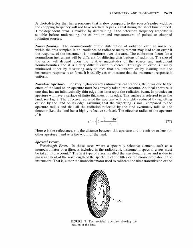
RADIOMETRY AND PHOTOMETRY 24 .39
A photodetector that has a response that is slow compared to the source’s pulse width or the chopping frequency will not have reached its peak signal during the short time interval . Time-dependent error is avoided by determining if the detector’s frequency response is suitable before undertaking the calibration and measurement of pulsed or chopped radiation sources .
Nonuniformity . The nonuniformity of the distribution of radiation over an image or within the area sampled in an irradiance or radiance measurement may lead to an error if the response of the instrument is nonuniform over this area . The calibration factor for a nonuniform instrument will be dif ferent for dif fering distributions of radiation . The size of the error will depend upon the relative magnitudes of the source and instrument nonuniformities and it is a very dif ficult error to correct . This type of error is usually minimized either by measuring only sources that are uniform or by insuring that the instrument response is uniform . It is usually easier to assure that the instrument response is uniform .
Nonideal Aperture . For very high-accuracy radiometric calibrations , the error due to the ef fect of the land on an aperture must be correctly taken into account . An ideal aperture is one that has an infinitesimally thin edge that intercepts the radiation beam . In practice an aperture will have a surface of finite thickness at its edge . This surface is referred to as the land ; see Fig . 7 . The ef fective radius of the aperture will be slightly reduced by vignetting caused by the land on its edge , assuming that the vignetting is small compared to the aperture radius and that all the radiation reflected by the land eventually falls on the detector (i . e ., the land has a highly reflective surface) . The ef fective radius of the aperture r 9 is
r 9 5 r F 1 2 (1 2 r ) w
s G (77)
Here r is the reflectance , s is the distance between this aperture and the mirror or lens (or other aperture) , and w is the width of the land .
Spectral Errors . Wa y elength Error . In those cases where a spectrally selective element , such as a
monochromator or a filter , is included in the radiometric instrument , spectral errors must be taken into account . 2 4 The first type of error is called the wavelength error and is due to misassignment of the wavelength of the spectrum of the filter or the monochromator in the instrument . That is , either the monochromator used to calibrate the filter transmission or the
FIGURE 7 The nonideal aperture showing the location of the land .
24 .40 OPTICAL MEASUREMENTS
monochromator within the radiometric instrument has an error in its wavelength setting . This error is eliminated by calibration of the monochromator wavelength setting using one or more atomic emission lines from either a discharge lamp (usually a mercury and / or a rare gas lamp) or one of the many spectra of the elements available as a hollow cathode lamp . The wavelengths of most atomic emission lines are known with an accuracy that exceeds the requirements of radiometric calibrations .
A special note regarding the wavelength error and the use of interference filters in a radiometric instrument . The typical angular sensitivity of an interference filter is 0 . 1 nm per angular degree of rotation . If the transmission of the interference filter is measured in a collimated beam and then used in a convergent beam there will be an error due to the angularly dependent shift in the spectral shape of the transmission . For an accurate radiometric instrument it is important to measure interference filter transmission in nearly the same geometry as it will be used . Furthermore , the temperature coef ficient of the transmission of an interference filter is about 0 . 2 nm K 2 1 . Therefore , it is also important in subsequent measurements to assure that the filter remains at the same temperature as that used during the calibration .
It should also be noted that in order to accurately determine the spectral transmission of a monochromator it is necessary to completely fill the aperture of the dispersing element in the monochromator . This usually means that the field of view of the monochromator must be filled by the beam from the spectral calibration instrument .
Out - of - band Radiation Error . The second type of spectral error is called the out-of-band or spectrally stray radiation error . This error is due to the radiation transmitted at both longer and shorter wavelengths that are beyond the edges of the principle transmission band of the filter or monochromator . This radiation is not taken into account if the limits in the integral in Eq . (11) are restricted to the edges of the principle transmission band . Although the relative amount of radiation transmitted at any wavelength beyond the edges of the principle transmission band may appear to be negligible with respect to the amount of radiation within the band , it is the spectrally total radiation that ‘‘leaks through’’ that is the error signal . It is therefore necessary to determine the transmission of the filter or monochromator over the entire spectrum of either the detector’s response and / or the light source’s output , whichever is greater . If the out-of-band radiation ef fect is small , it is possible to determine the correction factor from nominal values or limited accuracy measurements of the out-of-band spectra of the source , detector , and filter (monochromator) .
Temperature Dependence . The ef fect of temperature on the various elements in a radiometric instrument must not be overlooked . Unless the temperature of the instrument at the time of its calibration is maintained during subsequent applications , there may be substantial changes introduced in the instrument calibration factor that could well be above the uncertainty of its traceability to absolute SI units . The simple solution is to control the temperature of the system from the calibration to the subsequent measure- ments . A more practical solution is often to measure the relative change in the instrument calibration factor as a function of temperature and then apply this as a correction factor to account for the temperature dif ference in the subsequent measurements .
2 4 . 6 PHOTOMETRY
Definition and Scope
Photometry is the measurement of radiation in a way that characterizes its ef fectiveness in stimulating the normal human visual system . 4–5 , 80–82 Since visual sensation is a subjective experience , it is not directly quantifiable in absolute physical units . Attempts to quantify human visual sensation , therefore , were by comparison to various specified sources of
RADIOMETRY AND PHOTOMETRY 24 .41
light . The first sources used as standards were candles and later flames of prescribed construction . About the turn of the century , groups of incandescent lamps were selected as photometric standards and eventually a planckian radiator at a specific temperature was adopted by international agreement as the standard source . At present , the SI base unit for photometry , the candela , is no longer defined in terms of a given light source but is related to the radiant intensity by a multiplicative constant . Therefore , either an absolute source or detector can be used to establish an internationally recognized photometric calibration . Furthermore , there is no need for a human observer to ef fect a quantitative photometric measurement .
Photometry , as discussed here , is more precisely referred to as physical photometry to distinguish it from psychophysical photometry . Early photometric calibrations relied on human observers to compare an unknown light source to a standard . Presently , photometric calibrations are based on measurements using physical instruments . The instrument simulates human visual response either by having a detector with a spectral response that approximates that of the CIE standard observer or by using the CIE standard observer spectral response function in the data analysis .
Psychophysical photometry is the measurement of the ef fectiveness of light in individual observers and is more generally referred to as visual science . An individual’s visual system may dif fer from that of the CIE standard observer defined for physical photometry , and these dif ferences are sometimes important in experiments in visual science .
Photometry is restricted to the measurement of the magnitude of the visual sensation without regard to color , although it is well known that the perception of brightness is highly dependent on color in many circumstances . Measurement of the human response to color in terms of color matching is known as colorimetry . See Vol . I , Chap . 26 .
Under reasonable light levels , the human eye can detect a dif ference of as little as 0 . 5 percent between two adjacent fields of illumination . For fields of illumination which are not adjacent , or are viewed at substantially dif ferent times , the eye can only detect dif ferences of 10 to 20 percent . A discussion of the performance of the human visual system can be found in Vol . I , Chap . 25 . Extensive treatments of photometry can be found in Walsh , 7 7 and Wyszecki and Stiles . 7 8
Photopic , Scotopic , and Mesopic Vision
Electromagnetic radiation of suf ficient power and in the wavelength range from about 360 to 830 nm , will stimulate the human visual system and elicit a response from an observer . The spectral range given here is the range over which measurements in physical photometry are defined . The range of reasonably perceptible radiation is usually given as about 400 to 700 nm . After light enters through the optical system of the eye—the cornea , iris or pupil , lens , and vitreous humor—the next stage of the visual response occurs in the retina . The retina contains two types of receptor cells : cones , which are the dominant sensors when the eye is adapated to higher radiance levels of irradiation ( photopic vision) , and rods , the dominant sensors at lower radiance levels ( scotopic vision) . Between the higher and lower levels of light adaptation is the region of mesopic vision , the range of radiance levels where both cones and rods contribute in varying degrees to the visual process .
Three types of cones having dif ferent spectral sensitivity functions exist in the normal human eye . The brain is able to distinguish colors by comparison of the signals from the three cone types . Of the three cone types , only the middle- and long-wavelength-sensitive cones contribute to the photopic sensation of the radiation entering the eye . The relative spectral sensitivity functions of the photopically and scotopically adapted human eye have been measured for a number of observers . From averages of these measurements , a set of values has been adopted by international agreement as the spectral ef ficiency for the CIE
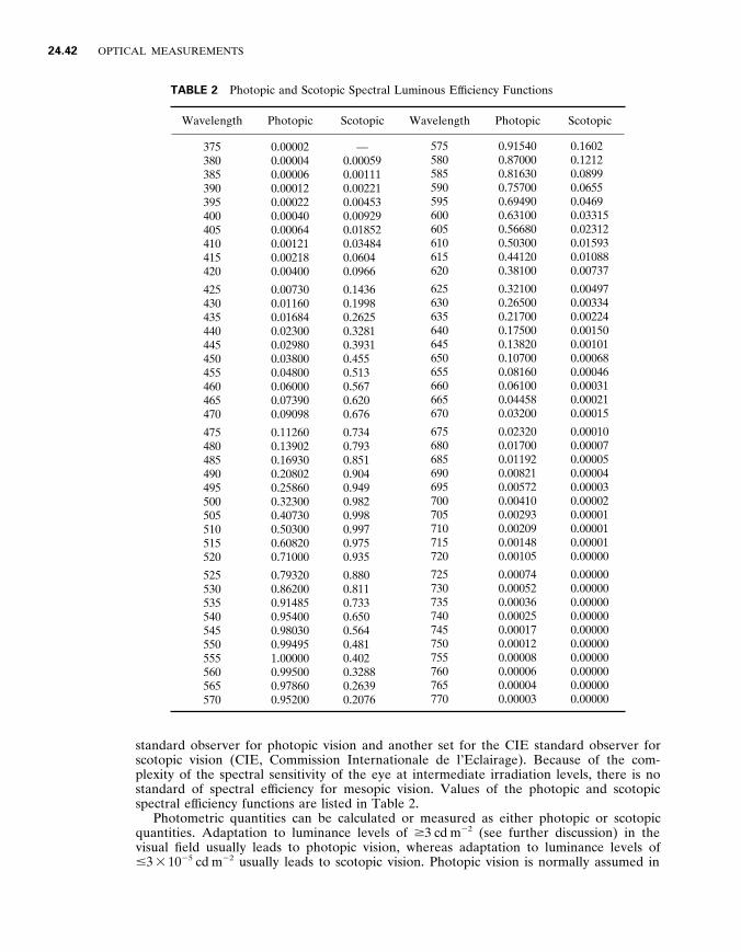
24 .42 OPTICAL MEASUREMENTS
TABLE 2 Photopic and Scotopic Spectral Luminous Ef ficiency Functions
Wavelength Photopic Scotopic Wavelength Photopic Scotopic
375 380 385 390 395 400 405 410 415 420
0 . 00002 0 . 00004 0 . 00006 0 . 00012 0 . 00022 0 . 00040 0 . 00064 0 . 00121 0 . 00218 0 . 00400
— 0 . 00059 0 . 00111 0 . 00221 0 . 00453 0 . 00929 0 . 01852 0 . 03484 0 . 0604 0 . 0966
425 430 435 440 445 450 455 460 465 470
0 . 00730 0 . 01160 0 . 01684 0 . 02300 0 . 02980 0 . 03800 0 . 04800 0 . 06000 0 . 07390 0 . 09098
0 . 1436 0 . 1998 0 . 2625 0 . 3281 0 . 3931 0 . 455 0 . 513 0 . 567 0 . 620 0 . 676
475 480 485 490 495 500 505 510 515 520
0 . 11260 0 . 13902 0 . 16930 0 . 20802 0 . 25860 0 . 32300 0 . 40730 0 . 50300 0 . 60820 0 . 71000
0 . 734 0 . 793 0 . 851 0 . 904 0 . 949 0 . 982 0 . 998 0 . 997 0 . 975 0 . 935
525 530 535 540 545 550 555 560 565 570
0 . 79320 0 . 86200 0 . 91485 0 . 95400 0 . 98030 0 . 99495 1 . 00000 0 . 99500 0 . 97860 0 . 95200
0 . 880 0 . 811 0 . 733 0 . 650 0 . 564 0 . 481 0 . 402 0 . 3288 0 . 2639 0 . 2076
575 580 585 590 595 600 605 610 615 620
0 . 91540 0 . 87000 0 . 81630 0 . 75700 0 . 69490 0 . 63100 0 . 56680 0 . 50300 0 . 44120 0 . 38100
0 . 1602 0 . 1212 0 . 0899 0 . 0655 0 . 0469 0 . 03315 0 . 02312 0 . 01593 0 . 01088 0 . 00737
625 630 635 640 645 650 655 660 665 670
0 . 32100 0 . 26500 0 . 21700 0 . 17500 0 . 13820 0 . 10700 0 . 08160 0 . 06100 0 . 04458 0 . 03200
0 . 00497 0 . 00334 0 . 00224 0 . 00150 0 . 00101 0 . 00068 0 . 00046 0 . 00031 0 . 00021 0 . 00015
675 680 685 690 695 700 705 710 715 720
0 . 02320 0 . 01700 0 . 01192 0 . 00821 0 . 00572 0 . 00410 0 . 00293 0 . 00209 0 . 00148 0 . 00105
0 . 00010 0 . 00007 0 . 00005 0 . 00004 0 . 00003 0 . 00002 0 . 00001 0 . 00001 0 . 00001 0 . 00000
725 730 735 740 745 750 755 760 765 770
0 . 00074 0 . 00052 0 . 00036 0 . 00025 0 . 00017 0 . 00012 0 . 00008 0 . 00006 0 . 00004 0 . 00003
0 . 00000 0 . 00000 0 . 00000 0 . 00000 0 . 00000 0 . 00000 0 . 00000 0 . 00000 0 . 00000 0 . 00000
standard observer for photopic vision and another set for the CIE standard observer for scotopic vision (CIE , Commission Internationale de l’Eclairage) . Because of the com- plexity of the spectral sensitivity of the eye at intermediate irradiation levels , there is no standard of spectral ef ficiency for mesopic vision . Values of the photopic and scotopic spectral ef ficiency functions are listed in Table 2 .
Photometric quantities can be calculated or measured as either photopic or scotopic quantities . Adaptation to luminance levels of $ 3 cd m 2 2 (see further discussion) in the visual field usually leads to photopic vision , whereas adaptation to luminance levels of # 3 3 10 2 5 cd m 2 2 usually leads to scotopic vision . Photopic vision is normally assumed in
RADIOMETRY AND PHOTOMETRY 24 .43
photometric measurements and photometric calculations unless explicitly stated to be otherwise .
Basic Concepts and Terminology
As noted in the earlier section on ‘‘Photometry , ’’ the principles of photometry are the same as those for radiometry with the exception that the spectral responsivity of the detector is defined by general agreement to be specific approximations of the relative spectral response functions of the human eye . Photometric quantities are related to radiometric quantities via the spectral ef ficiency functions defined for the photopic and scotopic CIE standard observers .
Luminous Flux . If physical photometry were to have been invented after the beginning of the twentieth century , then the physical basis of measurement might well have been the relationship between visual sensations and the energy of the photons and their flux density . It would follow naturally because vision is a photobiological process that is more closely related to the quantum nature of the radiation rather than its thermal heating ef fects . However , because of the weight of historical precedent , the basis of physical photometry is defined as the relationship between visual sensation and radiant power and its wavelength . The photometric equivalent of radiant power is luminous flux , and the unit that is equivalent to the watt is the lumen .
Luminous flux , F y , is the quantity derived from spectral radiant power by evaluating the radiation according to its action upon the CIE standard observer .
F y 5 K m E F l V ( l ) d l (78)
where V ( l ) is the spectral ef ficiency function for photopic vision listed in Table 2 , and K m is the luminous ef ficacy for photopic vision . The spectral luminous ef ficacy is defined near the maximum , l m 5 555 nm , of the photopic ef ficiency function to be
K m 5 683 V ( l m )
V (555 . 016 nm) > 683 lm W 2 1 (79)
The definitions are similar for scotopic vision
F 9 y 5 K 9 m E F l V 9 ( l ) d l (80)
where V 9 ( l ) is the spectral luminous ef ficiency function for scotopic vision listed in Table 2 , and K 9 m is the luminous ef ficacy for scotopic vision . The scotopic luminous ef ficiency function maximum occurs at l m 5 507 nm . The defining equation for K 9 m is
K 9 m 5 683 V 9 ( l m )
V 9 (555 . 016 nm) > 1700 lm W 2 1 (81)
The spectral shifts indicated in Eqs . (79) and (81) are required in order to obtain the precise values for the photopic and scotopic luminous ef ficacies . The magnitudes of the
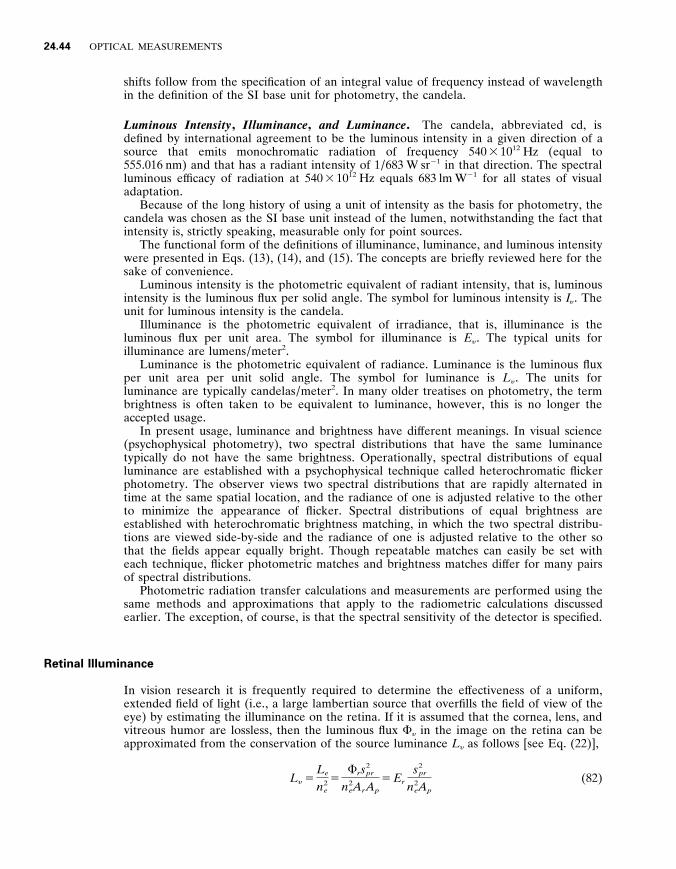
24 .44 OPTICAL MEASUREMENTS
shifts follow from the specification of an integral value of frequency instead of wavelength in the definition of the SI base unit for photometry , the candela .
Luminous Intensity , Illuminance , and Luminance . The candela , abbreviated cd , is defined by international agreement to be the luminous intensity in a given direction of a source that emits monochromatic radiation of frequency 540 3 10 1 2 Hz (equal to 555 . 016 nm) and that has a radiant intensity of 1 / 683 W sr 2 1 in that direction . The spectral luminous ef ficacy of radiation at 540 3 10 1 2 Hz equals 683 lm W 2 1 for all states of visual adaptation .
Because of the long history of using a unit of intensity as the basis for photometry , the candela was chosen as the SI base unit instead of the lumen , notwithstanding the fact that intensity is , strictly speaking , measurable only for point sources .
The functional form of the definitions of illuminance , luminance , and luminous intensity were presented in Eqs . (13) , (14) , and (15) . The concepts are briefly reviewed here for the sake of convenience .
Luminous intensity is the photometric equivalent of radiant intensity , that is , luminous intensity is the luminous flux per solid angle . The symbol for luminous intensity is I y . The unit for luminous intensity is the candela .
Illuminance is the photometric equivalent of irradiance , that is , illuminance is the luminous flux per unit area . The symbol for illuminance is E y . The typical units for illuminance are lumens / meter 2 .
Luminance is the photometric equivalent of radiance . Luminance is the luminous flux per unit area per unit solid angle . The symbol for luminance is L y . The units for luminance are typically candelas / meter 2 . In many older treatises on photometry , the term brightness is often taken to be equivalent to luminance , however , this is no longer the accepted usage .
In present usage , luminance and brightness have dif ferent meanings . In visual science (psychophysical photometry) , two spectral distributions that have the same luminance typically do not have the same brightness . Operationally , spectral distributions of equal luminance are established with a psychophysical technique called heterochromatic flicker photometry . The observer views two spectral distributions that are rapidly alternated in time at the same spatial location , and the radiance of one is adjusted relative to the other to minimize the appearance of flicker . Spectral distributions of equal brightness are established with heterochromatic brightness matching , in which the two spectral distribu- tions are viewed side-by-side and the radiance of one is adjusted relative to the other so that the fields appear equally bright . Though repeatable matches can easily be set with each technique , flicker photometric matches and brightness matches dif fer for many pairs of spectral distributions .
Photometric radiation transfer calculations and measurements are performed using the same methods and approximations that apply to the radiometric calculations discussed earlier . The exception , of course , is that the spectral sensitivity of the detector is specified .
Retinal Illuminance
In vision research it is frequently required to determine the ef fectiveness of a uniform , extended field of light (i . e ., a large lambertian source that overfills the field of view of the eye) by estimating the illuminance on the retina . If it is assumed that the cornea , lens , and vitreous humor are lossless , then the luminous flux F y in the image on the retina can be approximated from the conservation of the source luminance L y as follows [see Eq . (22)] ,
L y 5 L e
n 2 e 5
F r s 2 pr
n 2 e A r A p
5 E r s 2
pr
n 2 e A p
(82)
RADIOMETRY AND PHOTOMETRY 24 .45
where L e is the radiance within the eye , n e is the index of refraction of the ocular medium (the index of refraction of air is 1) , F r is the luminous flux at the retina , A r is the area of the image of the retina , A p is the area of the pupil , s p r is the distance from the pupil to the retina , and E r is the average illuminance in the image . Therefore , the average illuminance on the retina is
E r 5 L y
n 2 e A p
s 2 pr
(83)
The luminance can , of course , be in units of either photopic or scotopic cd m 2 2 . The area of the pupil is measurable , but the distance between the pupil and retina is typically not available . Therefore , a unit of retinal illuminance that avoids the necessity of determining this distance has been defined in terms of just the source luminance and pupil area . This unit is the troland , abbreviated td , and is defined as the retinal illumination for a pupil area of 1 mm 2 produced by a radiating surface having a luminance of 1 cd m 2 2 .
E T 5 L y A p (84)
Although it may be construed as an equivalent unit , one troland is not equal to one microcandela . The source is not a point but is infinite in extent . The troland is useful for relating several vision experiments where sources of dif fering luminance levels and pupil areas have been used .
The troland is , furthermore , not a measure of the actual illuminance level on the retina since the distance , index of refraction , and transmittance of the ocular medium are not included . For a schematic eye , which is designed to include many of the optical properties of the typical human eye , the ef fective distance between the pupil and the retina including the ef fect of the index of refraction is 16 . 7 mm 8 3 (see also Vol . I , Chap . 26) . For the schematic eye with a 1-mm 2 pupil area , the ef fective solid angle at the retina is approximately 0 . 0036 sr . The retinal illuminance equivalent to one troland is therefore 0 . 0036 lm m 2 2 times the ocular transmittance .
Recall from the section on ‘‘Radiometric Ef fects of Stops and Vignetting’’ the ef fect of the aperture stop on the light entering an optical system ; that is , all of the light entering the optical system appears to pass through the exit pupil , and the image of the aperture stop on the retina is the exit pupil . If the source is uniform and very large so that it overfills the field of view of the eye , the illuminance on the retina is independent of the distance between the source and the eye . If there is no intervening optic between the eye and the source , then the pupil is the aperture stop . However , if one uses an optical system to image the source into the eye , then the aperture stop need not be the pupil . An external optical system enables both the use of a more uniform , smaller source and the precise control of the retinal illumination by adjustment of an external aperture . The first configuration is called the newtonian view and the second is the maxwellian view of a source 8 0 (see also Vol . I , Chap . 28) .
Though the troland is a very useful and a commonly used photometric unit among vision researchers , it should be interpreted with some caution in situations where one wishes to draw quantitative inferences about the ef fect of light falling on the retina . The troland is not a precise predictor because , besides not including transmission losses , no angular information is conveyed . The photoreceptors exhibit directional sensitivity where light entering through the center of the pupil is more ef fective than light entering through the pupil margin (the Stiles-Crawford ef fect , see Vol . I , Chap . 24) . Finally , specifying retinal illuminance in photometric units of trolands does not completely define the experimental conditions because the spectral distribution of the light on the retina is unspecified . Rather , the relative spectral responsivity of the eye (including the spectral dependence of the transmittance) is assumed by the inclusion of the V ( l ) or V 9 ( l ) functions . Experiments performed under mesopic conditions will be particularly prone to error .
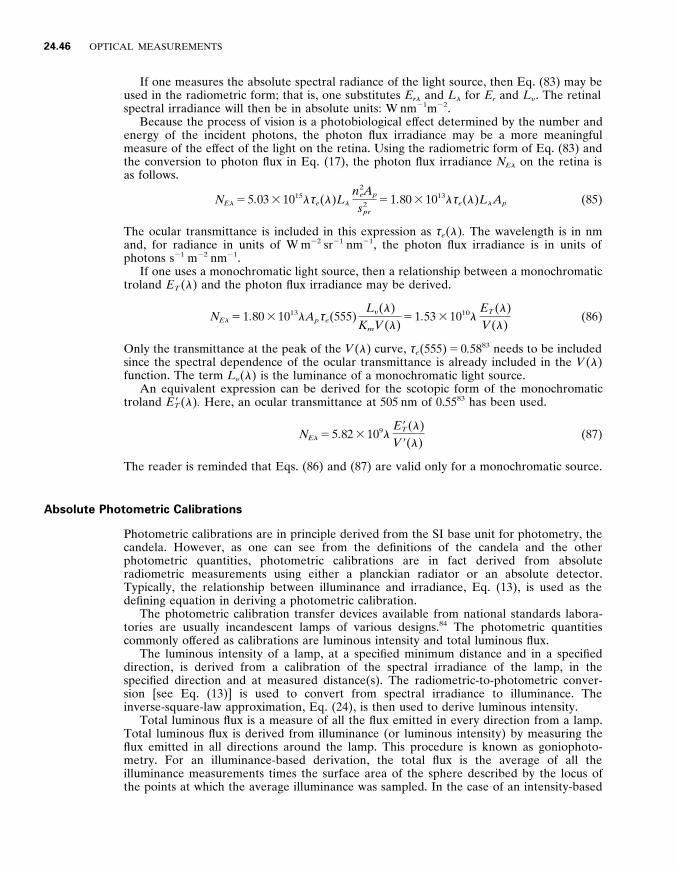
24 .46 OPTICAL MEASUREMENTS
If one measures the absolute spectral radiance of the light source , then Eq . (83) may be used in the radiometric form ; that is , one substitutes E r l and L l for E r and L y . The retinal spectral irradiance will then be in absolute units : W nm 2 1 m 2 2 .
Because the process of vision is a photobiological ef fect determined by the number and energy of the incident photons , the photon flux irradiance may be a more meaningful measure of the ef fect of the light on the retina . Using the radiometric form of Eq . (83) and the conversion to photon flux in Eq . (17) , the photon flux irradiance N E l on the retina is as follows .
N E l 5 5 . 03 3 10 1 5 l τ e ( l ) L l
n 2 e A p
s 2 pr
5 1 . 80 3 10 1 3 l τ e ( l ) L l A p (85)
The ocular transmittance is included in this expression as τ e ( l ) . The wavelength is in nm and , for radiance in units of W m 2 2 sr 2 1 nm 2 1 , the photon flux irradiance is in units of photons s 2 1 m 2 2 nm 2 1 .
If one uses a monochromatic light source , then a relationship between a monochromatic troland E T ( l ) and the photon flux irradiance may be derived .
N E l 5 1 . 80 3 10 1 3 l A p τ e (555) L y ( l )
K m V ( l ) 5 1 . 53 3 10 1 0 l
E T ( l ) V ( l )
(86)
Only the transmittance at the peak of the V ( l ) curve , τ e (555) 5 0 . 58 8 3 needs to be included since the spectral dependence of the ocular transmittance is already included in the V ( l ) function . The term L y ( l ) is the luminance of a monochromatic light source .
An equivalent expression can be derived for the scotopic form of the monochromatic troland E 9 T ( l ) . Here , an ocular transmittance at 505 nm of 0 . 55 8 3 has been used .
N E l 5 5 . 82 3 10 9 l E 9 T ( l ) V 9 ( l )
(87)
The reader is reminded that Eqs . (86) and (87) are valid only for a monochromatic source .
Absolute Photometric Calibrations
Photometric calibrations are in principle derived from the SI base unit for photometry , the candela . However , as one can see from the definitions of the candela and the other photometric quantities , photometric calibrations are in fact derived from absolute radiometric measurements using either a planckian radiator or an absolute detector . Typically , the relationship between illuminance and irradiance , Eq . (13) , is used as the defining equation in deriving a photometric calibration .
The photometric calibration transfer devices available from national standards labora- tories are usually incandescent lamps of various designs . 8 4 The photometric quantities commonly of fered as calibrations are luminous intensity and total luminous flux .
The luminous intensity of a lamp , at a specified minimum distance and in a specified direction , is derived from a calibration of the spectral irradiance of the lamp , in the specified direction and at measured distance(s) . The radiometric-to-photometric conver- sion [see Eq . (13)] is used to convert from spectral irradiance to illuminance . The inverse-square-law approximation , Eq . (24) , is then used to derive luminous intensity .
Total luminous flux is a measure of all the flux emitted in every direction from a lamp . Total luminous flux is derived from illuminance (or luminous intensity) by measuring the flux emitted in all directions around the lamp . This procedure is known as goniophoto- metry . For an illuminance-based derivation , the total flux is the average of all the illuminance measurements times the surface area of the sphere described by the locus of the points at which the average illuminance was sampled . In the case of an intensity-based
RADIOMETRY AND PHOTOMETRY 24 .47
derivation , the total flux is the average of all the intensity measurements times 4 π steradians . These are , in principle , the calculation methods for goniophotometry . In practice , the average illuminance (or intensity) is measured in a number of zones of fixed area (or solid angle) around the lamp . The product of the illuminance times the area of the zone (or the intensity times the solid angle of the zone) is the flux . The flux from each of the zones is then summed to obtain the total flux from the lamp .
A number of national standards laboratories provide luminance calibration transfer devices . These are typically in the form of a translucent glass plate that is placed at a specified distance and direction from a luminous intensity standard . One method of deriving the luminance calibration of the lamp / glass unit is to restrict the area of the glass plate with an aperture of known area . The intensity of the lamp / glass combination is then calibrated by comparison to an intensity standard lamp and the average luminance calculated by dividing the measured intensity by the area of the aperture .
Some national standards laboratories also of fer calibrations of photometers , 8 5 also known as illuminance meters . A photometer is a photodetector that has been fitted with a filter to tailor its relative (peak normalized) spectral responsivity to match that of the CIE standard photopic observer . Calibration of a photometer is usually obtained by reference to a luminous intensity standard positioned at a measured distance from the detector aperture . The inverse-square-law approximation is invoked to obtain the value of the illuminance at the measurement distance .
Other Photometric Terminology
Foot - candles , Foot - lamberts , Nits , etc . The following units of illuminance are often used in photometry , particularly in older texts :
lux (abbreviation : lx) 5 lumen per square meter phot (abbreviation : ph) 5 lumen per square centimeter meter candle 5 lumen per square meter footcandle (abbreviation : fc) 5 lumen per square foot
One foot-candle 5 0 . 0929 lux . The following units of luminance are often used :
nit (abbreviation : nt) 5 candela per square meter stilb (abbreviation : sb) 5 candela per square centimeter
It is sometimes the practice , particularly in illuminating engineering , to express the luminance of an actual surface in any given direction in relation to the luminance of a uniform , dif fuse , i . e ., lambertian , source that emits one lumen per unit area into a solid angle of π steradians [see Eq . (30)] . This concept is one of relative luminance and its units (given following) are not equatable to the units of luminance . Furthermore , in spite of what may appear to be a similarity , this concept is not , strictly speaking , the photometric equivalent of the exitance of a source because , in its definition , the integral of the flux over the entire hemisphere is referenced . In other words , the equivalence to emittance is true only for a perfectly uniform radiance source . For all other sources it is the luminance in a particular direction divided by π . The units for luminance normalized to a lambertian source are :
1 apostilb (abbreviation : asb) 5 (1 / π ) candela per square meter 1 lambert (abbreviation : L) 5 (1 / π ) candela per square centimeter 1 foot-lambert (abbreviation : fL) 5 (1 / π ) candela per square foot
24 .48 OPTICAL MEASUREMENTS
Sometimes the total flux of a source is referred to as its candlepower or spherical candlepower . This term refers to a point source that uniformly emits in all directions , that is , into a solid angle of 4 π steradians . Such a source does not exist , of course , so that the terminology is more precisely stated as the mean spherical candle power , which is the mean value of the intensity of the source averaged over the total solid angle subtended by a sphere surrounding the source .
Distribution Temperature , Color Temperature . Distribution temperature is an ap- proximate characterization of the spectral distribution of the visible radiation of a light source . Its use is restricted to sources having relative spectral outputs similar to that of a blackbody such as an incandescent lamp . The mathematical expression for evaluating distribution temperature is
E l 2
l 1
F 1 2 f x ( l )
a f b ( l , T ) G 2
d l é minimum (88)
where f x ( l ) is the relative spectral radiant power distribution function of the test source , f b ( l , T ) is the relative spectral radiant power distribution function of a blackbody at the temperature T , and a is an arbitrary constant . The limits of integration are the limits of visible radiation . Since distribution temperature is only an approximation , the exact values of the integration limits are arbitrary : typical limits are 400 and 750 nm . Values of a and T are adjusted simultaneously until the value of the integral is minimized . The temperature of the best-fit blackbody function is the distribution temperature .
Color temperature and correlated color temperature are defined in terms of the perceived color of a source and are obtained by determining the chromaticity of the radiation rather than its relative spectral distribution . Because they are not related to physical photometry they are not defined in this section of the Handbook . These quantities do not provide information about the spectral distribution of the source except when the source has an output that closely approximates a blackbody . Although widely , and mistakenly , used in general applications to characterize the relative spectral radiant power distribution of light sources , color temperature and correlated color temperature relate only to the three types of cone cell receptors for photopic human vision and the approximate manner in which the human brain processes these three signals . As examples of incompatibility , there are the obvious dif ferences between the spectral sensitivity of the human eye and physical receptors of visible optical radiation , e . g ., photographic film , TV cameras . In addition , ambiguities occur in the ability of humans to distinguish the perceived color from dif ferent spectral distributions (metameric pairs) . These ambiguities and the spectral sensitivity functions of the eye are not replicated by physical measurement systems . Caution must be exercised when using color temperature or correlated color temperature to predict the performance of a physical measurement system .
2 4 . 7 REFERENCES
1 . M . Born and E . Wolf , Principles of Optics , 6th ed ., Pergamon , Oxford , 1980 . 2 . E . Wolf , ‘‘Coherence and Radiometry , ’’ J . Opt . Soc . Am . 68 : 6 (1978) . 3 . J . Geist , McGraw - Hill Encyclopedia of Science and Technology , McGraw-Hill , New York , 1987 ,
p . 156 . 4 . W . Blevin et al ., ‘‘Principles Governing Photometry , ’’ Metrologia 19 : 97 (1983) . 5 . ‘‘The Basis of Physical Photometry , ’’ 2d ed ., Commission International de L ’ Eclairage Publ . No .
1 8 . 2 , Central Bureau of the CIE , Vienna , 1983 . 6 . R . W . Boyd , Radiometry and the Detection of Optical Radiation , Wiley , New York , 1983 .
RADIOMETRY AND PHOTOMETRY 24 .49
7 . F . Grum and R . J . Becherer , Optical Radiation Measurements , Academic Press , New York 1979 . 8 . F . Hengstberger , ed . Absolute Radiometry , Academic Press , New York , 1989 . 9 . C . L . Wyatt , Radiometric Calibration : Theory and Methods , Academic Press , New York , 1978 .
10 . E . L . Dereniak and D . G . Crowe , Optical Radiation Detectors , Wiley , New York , 1984 , pp . 1 – 14 , and Apps . A and C .
11 . M . V . Klein and T . E . Furtak , Optics , 2d ed ., Wiley , New York , 1986 , pp . 203 – 222 . 12 . T . J . Quinn , Temperature , Academic Press , New York , 1983 , pp . 284 – 363 . 13 . W . S . Smith , Modern Optical Engineering , 2d ed ., McGraw-Hill , New York , 1990 , pp . 135 – 136 ,
142 – 145 , and 205 – 231 . 14 . M . E . Chahine , D . J . McCleese , P . W . Rosenkranz , and D . H . Staelin , in Manual of Remote
Sensing , 2d ed ., American Society of Photogrammetry , Falls Church , VA , 1983 , pp . 172 – 179 . 15 . J . E . Hansen and L . D . Travis , ‘‘Light Scattering in Planetary Atmospheres , ’’ Space Science
Re y iews 16 : 527 (1974) . 16 . Y . J . Kaufman , in Ghassem Asrar (ed . ) , Theory and Applications of Optical Remote Sensing ,
Wiley , New York , 1989 , pp . 350 – 378 . 17 . H . Y . Wong , Handbook of Essential Formulae and Data on Heat Transfer for Engineers ,
Longman , London , 1977 , pp . 89 – 128 . 18 . E . M . Sparrow and R . D . Cess , Radiation Heat Transfer , Brooks-Cole , Belmont , CA , 1966 . 19 . D . G . Goebel , ‘‘Generalized Integrating Sphere Theory , ’’ Appl . Opt . 6 : 125 (1967) . 20 . ‘‘Le Syste me International d’Unite s , ’’ 3d ed ., Bureau International des Poids et Mesures , Se vres ,
France , 1977 . 21 . J . H . Walker , R . D . Saunders , J . K . Jackson , and D . A . McSparron , Spectral Irradiance
Calibrations , National Bureau of Standards Special Publication No . 250-20 , U . S . Government Printing Of fice , Washington , D . C ., 1987 .
22 . L . P . Boivin , ‘‘Calibration of Incandescent Lamps for Spectral Irradiance by Means of Absolute Radiometers , ’’ Appl . Opt . 19 : 2771 (1980) .
23 . E . F . Zalewski and W . K . Gladden , ‘‘Absolute Spectral Irradiance Measurements Based on the Predicted Quantum Ef ficiency of a Silicon Photodiode , ’’ Opt . Pura y Aplicada 17 : 133 (1984) .
24 . L . P . Boivin and A . A . Gaertner , ‘‘Realization of a Spectral Irradiance Scale in the Near Infrared at the National Research Council of Canada , ’’ Appl . Opt . 28 : 6082 (1992) .
25 . A . M . Mood and F . A . Graybill , Introduction to the Theory of Statistics , McGraw-Hill , New York , 1963 .
26 . G . W . Snedecor and W . G . Cochran , Statistical Methods , Iowa State Univ . Press , Ames , Iowa , 1967 .
27 . E . B . Wilson , Jr ., An Introduction to Scientific Research , McGraw-Hill , New York , 1952 . 28 . H . P . Baltes and E . R . Hilf , Spectra of Finite Systems , Bibliographisches Institut Manheim ,
Vienna , Zurich , 1976 . 29 . H . P . Baltes , ‘‘Deviations from the Stefan-Boltzmann Law at Low Temperatures , ’’ Appl . Phys .
1 : 39 (1973) . 30 . H . P . Baltes , ‘‘Planck’s Law for Finite Cavities and Related Problems , ’’ Infrared Phys . 16 : 1 (1976) . 31 . E . M . Sparrow , L . U . Ulbers , and E . R . Eckert , ‘‘Thermal Radiation Characteristics of Cylindrical
Enclosures , ’’ J . Heat Transfer C84 : 188 (1962) . 32 . B . A . Peavy , ‘‘A Note on the Numerical Evaluation of Thermal Radiation Characteristics of
Dif fuse Cylindrical and Conical Cavities , ’’ J . Res . Natl . Bur , Stds . 70C : 139 (1966) . 33 . R . E . Bedford and C . K . Ma , ‘‘Emissivities of Dif fuse Cavities : Isothermal and Non-isothermal
Cones and Cylinders , ’’ J . Opt . Soc . Amer . 64 : 339 (1974) . 34 . R . E . Bedford and C . K . Ma , ‘‘Emissivities of Dif fuse Cavities , II : Isothermal and Non-isothermal
Cylindro-cones , ’’ J . Opt . Soc . Amer . 65 : 565 (1975) . 35 . R . E . Bedord and C . K . Ma , ‘‘Emissivities of Dif fuse Cavities , III : Isothermal and Non-isothermal
Double Cones’’ , J . Opt . Soc . Amer . 66 : 724 (1976) .
24 .50 OPTICAL MEASUREMENTS
36 . J . C . de Vos , ‘‘Evaluation of the Quality of a Blackbody , ’’ Physica 20 : 669 (1954) . 37 . T . J . Quinn , ‘‘The Calculation of the Emissivity of Cylindrical Cavities Giving Near Blackbody
Radiation , ’’ Brit . J . Appl . Phys . 18 : 1105 (1967) . 38 . E . M . Sparrow and V . K . Johnson , ‘‘Absorption and Emission Characteristics of Dif fuse Spherical
Enclosures , ’’ J . Heat Transfer C84 : 188 (1962) . 39 . T . J . Quinn , ‘‘The Absorptivity of a Specularly Reflecting Cone for Oblique Angles of View , ’’
Infrared Phys . 21 : 123 (1981) . 40 . T . J . Quinn and J . E . Martin , ‘‘Blackbody Source in the 2 50 to 1 200 8 C Range for the Calibration
of Radiometers and Radiation Thermometers , ’’ Appl . Opt . 30 : 4486 (1991) . 41 . E . F . Zalewski , J . Geist , and R . C . Willson , ‘‘Cavity Radiometer Reflectance , ’’ Proc . of the SPIE
196 : 152 (1979) . 42 . J . Schwinger , ‘‘On the Classical Radiation of Accelerated Electrons , ’’ Phs . Re y . 75 : 1912 (1949) . 43 . D . H . Tomboulian and P . L . Hartman , ‘‘Spectral and Angular Distribution of Ultraviolet
Radiation from the 300-Mev Cornell Synchrotron , ’’ Phys . Re y . 102 : 1423 (1956) . 44 . D . Lemke and D . Labs , ‘‘The Synchrotron Radiation of the 6-Gev DESY Machine as a
Fundamental Radiometric Standard , ’’ Appl . Opt . 6 : 1043 (1967) . 45 . N . P . Fox , P . J . Key , P . J . Riehle , and B . Wende , ‘‘Intercomparison Between Two Independent
Primary Radiometric Standards in the Visible and near Infrared : a Cryogenic Radiometer and the Electron Storage Ring BESSY , ’’ Appl . Opt . 25 : 2409 (1986) .
46 . T . J . Quinn and J . E . Martin , ‘‘A Radiometric Determination of the Stefan-Boltzmann Constant and Thermodynamic Temperatures Between 2 40 8 C and 1 100 8 C , ’’ Phil . Trans . Roy . Soc . London 316 : 85 (1985) .
47 . V . E . Anderson and N . P . Fox , ‘‘A New Detector-based Spectral Emission Scale , ’’ Metrologia 28 : 135 (1991) .
48 . N . P . Fox , J . E . Martin , and D . H . Nettleton , ‘‘Absolute Spectral Radiometric Determination of the Melting / freezing Points of Gold , Silver and Aluminum , ’’ Metrologia 28 : 357 (1991) .
49 . L . Jauniskis , P . Foukal , and H . Kochling , ‘‘Absolute Calibration of an Ultraviolet Spectrometer Using a Stabilized Laser and a Cryogenic Radiometer , ’’ Appl . Opt . 31 : 5838 (1992) .
50 . F . Kurlbaum , ‘‘U ber eine Methode zur Bestimmung der Strahlung in Absolutem Maass un die Strahlung des schwarzen Ko pers zwischen 0 und 100 Grad , ’’ Wied . Ann . 65 : 746 (1898) .
51 . K . A ngstrom , ‘‘The Absolute Determination of the Radiation of Heat with the Electrical Compensation Pyrheliometer , with Examples of the Application of this Instrument , ’’ Astrophys . J . 9 : 332 (1899) .
52 . W . R . Blevin and W . J . Brown , ‘‘Development of a Scale of Optical Radiation , ’’ Austr . J . Phys . 20 : 567 (1967) .
53 . R . C . Willson , ‘‘Active Cavity Radiometer Type V , ’’ Appl . Opt . 19 : 3256 (1980) . 54 . L . P . Boivin and F . T . McNeely , ‘‘Electrically Calibrated Absolute Radiometer Suitable for
Measurement Automation , ’’ Appl . Opt . 25 : 554 (1986) . 55 . J . Geist and W . R . Blevin , ‘‘Chopper-stabilized Radiometer Based on an Electrically Calibrated
Pyroelectric Detector , ’’ Appl . Opt . 12 : 2532 (1973) . 56 . R . J . Phelan and A . R . Cook , ‘‘Electrically Calibrated Pyroelectric Optical-radiation Detector , ’’
Appl . Opt . 12 : 2494 (1973) . 57 . J . E . Martin , N . P . Fox , and P . J . Key , ‘‘A Cryogenic Radiometer for Absolute Radiometric
Measurements , ’’ Metrologia 21 : 147 (1985) . 58 . C . C . Hoyt and P . V . Foukal , ‘‘Cryogenic Radiometers and Their Application to Metrology , ’’
Metrologia 28 : 163 (1991) . 59 . J . A . R . Samson , ‘‘Absolute Intensity Measurements in the Vacuum Ultraviolet , ’’ J . Opt . Soc .
Amer . 54 : 6 (1964) . 60 . F . M . Matsunaga , R . S . Jackson , and K . Watanabe , ‘‘Photoionization Yield and Absorption
Coef ficient of Xenon in the Region of 860 – 1022 Å , ’’ J . Quant . Spectrosc . Radiat . Transfer 5 : 329 (1965) .
RADIOMETRY AND PHOTOMETRY 24 .51
61 . J . Geist , ‘‘Quantum Ef ficiency of the p – n Junction in Silicon as an Absolute Radiometric Standard , ’’ Appl . Opt . 18 : 760 (1979) .
62 . J . Geist , W . K . Gladden , and E . F . Zalewski , ‘‘The Physics of Photon Flux Measurements with Silicon Photodiodes , ’’ J . Opt . Soc . Amer . 72 : 1068 (1982) .
63 . E . F . Zalewski and J . Geist , ‘‘Silicon Photodiode Absolute Spectral Response Self-calibration , ’’ Appl . Opt . 19 : 1214 (1980) .
64 . J . Geist , E . F . Zalewski , and A . R . Schaefer , ‘‘Spectral Response Self-calibration and Interpolation of Silicon Photodiodes , ’’ Appl . Opt . 19 : 3795 (1980) .
65 . J . L . Gardner and W . J . Brown , ‘‘Silicon Radiometry Compared to the Australian Radiometric Scale , ’’ Appl . Opt . 26 : 2341 (1987) .
66 . E . F . Zalewski and C . C . Hoyt , ‘‘Comparison Between Cryogenic Radiometry and the Predicted Quantum Ef ficiency of Silicon Photodiode Light Traps , ’’ Metrologia 28 : 203 (1991) .
67 . E . F . Zalewski and C . R . Duda , ‘‘Silicon Photodiode Device with 100 Percent External Quantum Ef ficiency , ’’ Appl . Opt . 22 : 2867 (1983) .
68 . N . P . Fox , ‘‘Trap Detectors and Their Properties , ’’ Metrologia 28 : 197 (1991) . 69 . J . H . Walker , R . D . Saunders , and A . T . Hattenburg , Spectral Radiance Calibrations , National
Bureau of Standards Special Publication No . 250-1 , U . S . Government Printing Of fice , Washing- ton , D . C ., 1987 .
70 . J . Z . Klose , J . M . Bridges , and W . R . Ott , Radiometric Standards in the Vacuum Ultra y iolet , National Bureau of Standards Special Publication No . 250-3 , U . S . Government Printing Of fice , Washington , D . C ., 1987 .
71 . E . F . Zalewski , The NBS Photodetector Spectral Response Calibration Transfer Program , National Bureau of Standards Special Publication No . 250-17 , U . S . Government Printing Of fice , Washin- gton , D . C ., 1987 .
72 . W . Budde , Physical Detectors of Optical Radiation , Academic Press , New York , 1983 . 73 . L . P . Boivin , ‘‘Some Aspects of Radiometric Measurements Involving Gaussian Laser Beams , ’’
Metrologia 17 : 19 (1981) . 74 . L . P . Boivin , ‘‘Reduction of Dif fraction Errors in Radiometry by Means of Toothed Apertures , ’’
Appl . Opt . 17 : 3323 (1978) . 75 . W . R . Blevin , ‘‘Dif fraction Losses in Photometry and Radiometry , ’’ Metrologia 6 : 31 (1970) . 76 . C . L . Sanders , ‘‘A Photocell Linearity Tester , ’’ Appl . Opt . 1 : 207 (1962) . 77 . C . L . Sanders , ‘‘Accurate Measurements of and Corrections for Non-linearities in Radiometers , ’’
J . Res . Natl . Bur . Stand . A76 : 437 (1972) . 78 . W . Budde , ‘‘Multidecade Linearity Measurements on Silicon Photodiodes , ’’ Appl . Opt . 18 : 1555
(1979) . 79 . A . R . Schaefer , E . F . Zalewski , and J . Geist , ‘‘Silicon Detector Non-linearity and Related
Ef fects , ’’ Appl . Opt . 22 : 1232 (1983) . 80 . J . W . T . Walsh , Photometry , Dover , New York , 1965 . 81 . G . Wyszecki and W . S . Stiles , Colour Science : Concepts and Methods , Wiley , New York , 1967 . 82 . ‘‘Light as a True Visual Quantity : Principles of Measurement , ’’ Commission International de
L ’ Eclairage Publ . No . 4 1 , Central Bureau of the CIE , Vienna , 1978 . 83 . E . N . Pugh , ‘‘Vision : Physics and Retinal Physiology , ’’ in R . C . Atkinson , R . J . Herrnstein , G .
Lindsey , and R . D . Luce , eds ., Steven’s Handbook of Experimental Psychology , 2d ed ., Wiley , New York , 1988 , pp . 75 – 163 .
84 . R . L . Booker and D . A . McSparron , Photometric Calibrations , National Bureau of Standards Special Publication No . 250 – 15 , U . S . Government Printing Of fice , Washington , D . C ., 1987 .
85 . ‘‘Methods of Characterizing the Performance of Radiometers and Photometers , ’’ Commission International de L ’ Eclairage Publ . No . 5 3 , Central Bureau of the CIE , Vienna , 1982 .