Chapter 1 - Handbook of Optics -...

P d A d R d T d 1

OPTICAL ELEMENTS

CHAPTER 1 LENSES

R . Barry Johnson Optical E .T .C . , Inc . Hunts y ille , Alabama and Center for Applied Optics Uni y ersity of Alabama in Hunts y ille Hunts y ille , Alabama

1 . 1 GLOSSARY

AChr axial chromatic aberration

AST astigmatism b factor

bfl back focal length

C o scaling factor

c curvature C 1 scaling factor

C 2 scaling factor

CC conic constant

CMA s sagittal coma

CMA t tangential coma

D e p diameter of entrance pupil

d o distance from object to loupe

d e distance from loupe to the eye

E irradiance

efl ef fective focal length

ep eyepiece

FN F-number

f focal length

h height above axis

H i height of ray intercept in image plane

1 .3

1 .4 OPTICAL ELEMENTS

_ shape factor

i image

J 1 () Bessel function of the first kind

k 2 π / l L length

MP magnifying power [cf . linear lateral longitudinal magnification]

m linear , lateral magnification

m # linear , longitudinal , magnification

n refractive index

factor

MTF modulation transfer function

NA numerical aperture

a ,b first and second lenses

o object

obj objective

P partial dispersion

P i principal points

p 5 s d / f a 5 peak normalized spectral weighting function

6 object to image distance

SA3 third-order spherical aberration

SAC secondary angular spectrum

s i image distance

s o t optical tube length

s o object distance

TPAC transverse primary chromatic aberration

t thickness

u slope

V Abbe number or reciprocal dispersion

y f -normalized reciprocal object distance 1 / s o f

x , y , z cartesian coordinates

b angular blur diameter

d depth of focus

z sag

D θ angular blur tolerance

LENSES 1 .5

θ field of view

l wavelength

… spatial frequency

f lens power

r radius

s standard deviation of the irradiance distribution

τ transmission

Ω normalized spatial frequency

1 . 2 INTRODUCTION

This section provides a basic understanding of using lenses for image formation and manipulation . The principles of image formation are reviewed first . The ef fects of lens shape , index of refraction , magnification , and F-number on the image quality of a singlet lens are discussed in some detail . Achromatic doublets and more complex lens systems are covered next . A representative variety of lenses is analyzed and discussed . Performance that may be expected of each class of lens is presented . The section concludes with several techniques for rapid estimation of the performance of lenses . Refer to Chap . 1 ‘‘Geometric Optics’’ in Vol . I , for further discussion of geometrical optics and aberrations .

1 . 3 BASICS

Figure 1 illustrates an image being formed by a simple lens . The object height is h o and the image height is h i , with u o and u i being the corresponding slope angles . It follows from the Lagrange invariant that the lateral magnification is defined to be

m ; h i

h o

5 ( nu ) o

( nu ) i (1)

where n o and n i are the refractive indices of the medium in which the object and image lie , respectively . By convention , a height is positive if above the optical axis and a ray angle is positive if its slope angle is positive . Distances are positive if the ray propagates left to right . Since the Lagrange invariant is applicable for paraxial rays , the angle nu

FIGURE 1 Imaging by a simple lens .


should be understood to mean n tan u . This interpretation applies to all paraxial computations . For an aplanatic lens , which is free of spherical aberration and linear coma , the magnification can be shown by the optical sine theorem to be given by

m ; h i

h o

5 n o sin u o

n i sin u i (2)

If the object is moved a small distance s o longitudinally , the corresponding displacement of the image s i can be found by the dif ferential form of the basic imaging equation and leads to an equation analogous to the Lagrange invariant . The longitudinal magnification is then defined as

m # ; s i

s o

5 ( nu 2 ) o

( nu 2 ) i

5 m 2 F n i

n o G (3)

The following example will illustrate one application of m and m # . Consider that a spherical object of radius r o is to be imaged as shown in Fig . 2 . The equation of the object is r 2

o 5 y 2 o 1 z 2 , where z is measured along the optical axis and is zero at the object’s center

of curvature . Letting the surface sag as measured from the vertex plane of the object be denoted as z o , the equation of the object becomes r 2

o 5 ( r o 2 z o ) 2 1 y 2 o since z 5 r o 2 z o . In

the region near the optical axis , z 2 o Ô r 2

o , which implies that r o < y 2 o / 2 z o . The image of the

object is expressed in the transverse or lateral direction by y i 5 my o and in the longitudinal or axial direction by z i 5 m # z o 5 z o m 2 ( n i / n o ) . In a like manner , the image of the spherical object is expressed as r i < ( y i )

2 / 2 z i . By substitution , the sag of the image is expressed by

r i ; n o y 2

o

2 n i z o

5 r o F n o

n i G (4)

Hence , in the paraxial region about the optical axis , the radius of the image of a spherical

FIGURE 2 Imaging of a spherical object by a lens .

LENSES 1 .7

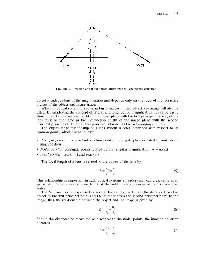
FIGURE 3 Imaging of a tilted object illustrating the Scheimpflug condition .

object is independent of the magnification and depends only on the ratio of the refractive indices of the object and image spaces .

When an optical system as shown in Fig . 3 images a tilted object , the image will also be tilted . By employing the concept of lateral and longitudinal magnification , it can be easily shown that the intersection height of the object plane with the first principal plane P 1 of the lens must be the same as the intersection height of the image plane with the second principal plane P 2 of the lens . This principle is known as the Scheimpflug condition .

The object-image relationship of a lens system is often described with respect to its cardinal points , which are as follows :

$ Principal points : the axial intersection point of conjugate planes related by unit lateral magnification

$ Nodal points : conjugate points related by unit angular magnification ( m 5 u i / u 0 ) $ Focal points : front ( f 1 ) and rear ( f 2 )

The focal length of a lens is related to the power of the lens by

f 5 n o

f o 5

n i

f i (5)

This relationship is important in such optical systems as underwater cameras , cameras in space , etc . For example , it is evident that the field of view is decreased for a camera in water .

The lens law can be expressed in several forms . If s o and s i are the distance from the object to the first principal point and the distance from the second principal point to the image , then the relationship between the object and the image is given by

f 5 n i

s i 1

n o

s o (6)

Should the distances be measured with respect to the nodal points , the imaging equation becomes

f 5 n o

s i 1

n i

s o (7)


When the distances are measured from the focal points , the image relationship , known as the Newtonian imaging equation , is given by

f 1 f 2 5 s o s i (8)

The power of a spherical refracting surface , with curvature c and n being the refractive index following the surface , is given by

f 5 c ( n 2 n o ) (9)

It can be shown that the power of a single thick lens in air is

f thick 5 f 1 1 f 2 2 f 1 f 2 t

n (10)

where t is the thickness of the lens . The distance from the first principal plane to the first surface is 2 ( t / n ) f 2 f 1 and the distance from the second principal point to the rear surface is ( 2 t / n ) f 1 f 2 . The power of a thin lens ( t 5 0) in air is given by

f thin 5 ( n 2 1)( c 1 2 c 2 ) (11)

1 . 4 STOPS AND PUPILS

The aperture stop or stop of a lens is the limiting aperture associated with the lens that determines how large an axial beam may pass through the lens . The stop is also called an iris . The marginal ray is the extreme ray from the axial point of the object through the edge of the stop . The entrance pupil is the image of the stop formed by all lenses preceding it when viewed from object space . The exit pupil is the image of the stop formed by all lenses following it when viewed from image space . These pupils and the stop are all images of one another . The principal ray is defined as the ray emanating from an of f-axis object point that passes through the center of the stop . In the absence of pupil aberrations , the principal ray also passes through the center of the entrance and exit pupils .

As the obliquity angle of the principal ray increases , the defining apertures of the components comprising the lens may limit the passage of some of the rays in the entering beam thereby causing the stop not to be filled with rays . The failure of an of f-axis beam to fill the aperture stop is called y ignetting . The ray centered between the upper and lower rays defining the oblique beam is called the chief ray . When the object moves to large of f-axis locations , the entrance pupil often has a highly distorted shape , may be tilted , and / or displaced longitudinally and transversely . Due to the vignetting and pupil aberrations , the chief and principal rays may become displaced from one another . In some cases , the principal ray is vignetted .

The field stop is an aperture that limits the passage of principal rays beyond a certain field angle . The image of the field stop when viewed from object space is called the entrance window and is called the exit window when viewed from image space . The field stop ef fectively controls the field of view of the lens system . Should the field stop be coincident with an image formed within or by the lens system , the entrance and exit windows will be located at the object and / or image(s) .

A telecentric stop is an aperture located such that the entrance and / or exit pupils are located at infinity . This is accomplished by placing the aperture in the focal plane . Consider a stop placed at the front focal plane of a lens . The image is located at infinity and the principal ray exits the lens parallel to the optical axis . This feature is often used in metrology since the measurement error is reduced when compared to conventional lens systems because the centroid of the blur remains at the same height from the optical axis even as the focus is varied .

LENSES 1 .9

1 . 5 F - NUMBER AND NUMERICAL APERTURE

The focal ratio or F-number (FN) of a lens is defined as the ef fective focal length divided by the entrance pupil diameter D e p . When the object is not located at infinity , the ef fective FN is given by

FN ef f 5 FN (1 2 m ) (12)

where m is the magnification . For example , for a simple positive lens being used at unity magnification ( m 5 2 1) , the FN ef f 5 2FN . The numerical aperture of a lens is defined as

NA 5 n i sin U i (13)

where n i is the refractive index in which the image lies and U i is the slope angle of the marginal ray exiting the lens . If the lens is aplanatic , then

FN ef f 5 1

2NA (14)

1 . 6 MAGNIFIER OR EYE LOUPE

The typical magnifying glass , or loupe , comprises a singlet lens and is used to produce an erect but virtual magnified image of an object . The magnifying power of the loupe is stated to be the ratio of the angular size of the image when viewed through the magnifier to the angular size without the magnifier . By using the thin-lens model of the human eye , the magnifying power (MP) can be shown to be given by

MP 5 25 cm

d e 1 d o 2 f d e d o (15)

where d o is the distance from the object to the loupe , d e is the separation of the loupe from the eye , and f 5 1 / f is the power of the magnifier . When d o is set to the focal length of the lens , the virtual image is placed at infinity and the magnifying power reduces to

MP 5 25 cm

f (16)

Should the virtual image be located at the near viewing distance of the eye (about 25 cm) , then

MP 5 25 cm

f 1 1 (17)

Typically simple magnifiers are dif ficult to make with magnifying powers greater than about 10 3 .

1 . 7 COMPOUND MICROSCOPES

For magnifying power greater than that of a simple magnifier , a compound microscope , which comprises an objective lens and an eyepiece , may be used . The objective forms an aerial image of the object at a distance s o t from the rear focal point of the objective . The


distance s o t is called the optical tube length and is typically 160 mm . The objective magnification is

MP o b j 5 s o t

f o b j (18)

The image formed is further magnified by the eyepiece which has a MP e p 5 250 mm / f e p . The total magnifying power of the compound microscope is given by

MP 5 MP obj MP e p

5 160 f o b j

? 250 f e p

(19)

Typically , f e p 5 25 mm , so its MP 5 10 . Should the objective have a focal length of 10 mm , the total magnifying power of the microscope is 16 3 times 10 3 , or 160 3 .

1 . 8 FIELD AND RELAY LENSES

Field lenses are placed at (or near) an image location for the purpose of optically relocating the pupil or to increase the field of view of the optical system . For example , a field lens may be used at the image plane of an astronomical telescope such that the field lens images the objective lens onto the eyepiece . In general , the field lens does not contribute to the aberrations of the system except for distortion and field curvature . Since the field lens must be positive , it adds inward curving Petzval . For systems having a small detector requiring an apparent increase in size , the field lens is a possible solution . The detector is located beyond the image plane such that it subtends the same angle as the objective lens when viewed from the image point . The field lens images the objective lens onto the detector .

Relay lenses are used to transfer an image from one location to another such as in a submarine periscope or borescope . It is also used as a means to erect an image in many types of telescopes and other such instruments . Often relay lenses are made using two lens groups spaced about a stop , or an image of the system stop , in order to take advantage of the principle of symmetry , thereby minimizing the comatic aberrations and lateral color . The relayed image is frequently magnified .

1 . 9 APLANATIC SURFACES AND IMMERSION LENSES

Abbe called a lens an aplanat that has an equivalent refractive surface which is a portion of a sphere with a radius r centered about the focal point . Such a lens satisfies the Abbe sine condition and implies that the lens is free of spherical and coma near the optical axis . Consequently , the maximum possible numerical aperture (NA) of an aplanat is unity , or an FN 5 0 . 5 . In practice , an FN less than 0 . 6 is dif ficult to achieve . For an aplanat ,

FN 5 1

2 ? NA (20)

It can be shown that three cases exist where the spherical aberration is zero for a spherical surface . These are : (1) the trivial case where the object and image are located at the surface , (2) the object and image are located at the center of curvature of the surface , and (3) the object is located at the aplanatic point . The third case is of primary interest . If

LENSES 1 .11

FIGURE 4 Aplanatic hemispherical magnifier with the object and image located at the center of curvature of the spherical surface . This type of magnifier has a magnification of n i / n o which can be used as a contact magnifier or as an immersion lens .

FIGURE 5 Aplanatic hyperhemispherical magnifier or Amici lens has the object located at the aplanatic point . The lateral magnification is ( n i / n 0 ) 2 .

the refractive index preceding the surface is n o and following the surface is n i , then the object is located a distance s o from the surface as expressed by

s o 5 r ( n o 1 n i )

n o (21)

and the image is located at

s i 5 r ( n o 1 n i )

n i (22)

An immersion lens or contact lens can be formed from an aplanatic surface and a plano surface . Figure 4 illustrates a hemispherical magnifier that employs the second aplanatic case . The resultant magnification is n i if in air or n i / n o otherwise . A similar magnifier can be constructed by using a hyperhemispherical surface and a plano surface as depicted in Fig . 5 . The lateral magnification is n 2

i . This lens , called an Amici lens , is based upon the third aplanatic case . The image is free of all orders of spherical aberration , third-order coma , and third-order astigmatism . Axial color is also absent from the hemispherical magnifier . These magnifiers are often used as a means to make a detector appear larger and as the first component in microscope objectives .

1 . 1 0 SINGLE ELEMENT LENS

It is well known that the spherical aberration of a lens is a function of its shape factor or bending . Although several definitions for the shape factor have been suggested , a useful formulation is

_ 5 c 1

c 1 2 c 2 (23)

where c 1 and c 2 are the curvatures of the lens with the first surface facing the object . By adjusting the lens bending , the spherical aberration can be seen to have a minimum value .


The power of a thin lens or the reciprocal of its focal length is given by

f 5 ( n 2 1) c 1

_ (24)

When the object is located at infinity , the shape factor for minimum spherical aberration can be represented by

_ 5 n (2 n 1 1) 2( n 1 2)

(25)

The resultant third-order spherical aberration of the marginal ray in angular units is

SA3 5 n 2 2 (2 n 1 1) _ 1 (1 1 2 / n ) _ 2

16( n 2 1) 2 (FN) 3 (26)

or after some algebraic manipulations ,

SA3 5 n (4 n 2 1)

64( n 1 2)( n 2 1) 2 (FN) 3 (27)

where , for a thin lens , the FN is the focal length f divided by the lens diameter , which in this case is the same as entrance pupil diameter D e p . Inspection of this equation illustrates that smaller values of spherical aberration are obtained as the refractive index increases .

When the object is located at a finite distance s o , the equations for the shape factor and residual spherical aberration are more complex . Recalling that the magnification m is the ratio of the object distance to the image distance and that the object distance is negative if the object lies to the left of the lens , the relationship between the object distance and the magnification is

1 s o f

5 m

1 2 m (28)

where m is negative if the object distance and the lens power have opposite signs . The term 1 / s o f represents the reduced or f -normalized reciprocal object distance y , i . e ., s o is measured in units of focal length f 2 1 . The shape factor for minimum spherical aberration is given by

_ 5 n (2 n 1 1) 2( n 1 2)

1 2( n 2 2 1)

n 1 2 S m

1 2 m D (29)

and the resultant third-order spherical aberration of the marginal ray in angular units is

SA3 5 1

16( n 2 1) 2 (FN) 3 F n 2 2 (2 n 1 1) _ 1 n 1 2

n _ 2 1 (3 n 1 1)( n 2 1) S m

1 2 m D

2 4( n 2 2 1)

n S m

1 2 m D _ 1

(3 n 1 2)( n 2 1) 2

n S m

1 2 m D 2 G (30)

where FN is the ef fective focal length of the lens f divided by its entrance pupil diameter . When the object is located at infinity , the magnification becomes zero and the above two equations reduce to those previously given .

LENSES 1 .13

FIGURE 6 The shape factor for a single lens is shown for several refractive indexes as a function of reciprocal object distance y where the distance is measured in units of focal length .

Figure 6 illustrates the variation in shape factor as a function of y for refractive indices of 1 . 5 – 4 for an FN 5 1 . As can be seen from the figure , lenses have a shape factor of 0 . 5 regardless of the refractive index when the magnification is 2 1 or y 5 2 0 . 5 . For this shape factor , all lenses have biconvex surfaces with equal radii . When the object is at infinity and the refractive index is 4 , lenses have a meniscus shape towards the image . For a lens with a refractive index of 1 . 5 , the shape is somewhat biconvex , with the second surface having a radius about 6 times greater than the first surface radius .

Since the minimum-spherical lens shape is selected for a specific magnification , the spherical aberration will vary as the object-image conjugates are adjusted . For example , a lens having a refractive index of 1 . 5 and configured for m 5 0 exhibits a substantial increase in spherical aberration when the lens is used at a magnification of 2 1 . Figure 7 illustrates the variation in the angular spherical aberration as both a function of refractive index and reciprocal object distance y when the lens bending is for minimum spherical aberration with the object located at infinity . As can be observed from Fig . 7 , the ratio of the spherical aberration , when m 5 2 0 . 5 and m 5 0 , increases as n increases . Figure 8 shows the variation in angular spherical aberration when the lens bending is for minimum spherical aberration at a magnification of 2 1 . In a like manner , Fig . 9 presents the variation in angular spherical aberration for a convex-plano lens with the plano side facing the image . The figure can also be used when the lens is reversed by simply replacing the object distance with the image distance .

Figures 7 – 9 may provide useful guidance in setting up experiments when the three forms of lenses are available . The so-called ‘‘of f-the-shelf’’ lenses that are readily available from a number of vendors often have the convex-plano , equal-radii biconvex , and minimum spherical shapes .

Figure 10 shows the relationship between the third-order spherical aberration and coma , and the shape factor for a thin lens with a refractive index of 1 . 5 , stop in contact , and the object at infinity . The coma is near zero at the minimum spherical aberration shape . The shape of the lens as a function of shape factor is shown at the top of the figure .

For certain cases , it is desirable to have a single lens with no spherical aberration . A


FIGURE 7 Variation of angular spherical aberration as a function of reciprocal object distance y for various refractive indices when the lens is shaped for minimum spherical aberration with the object at infinity . Spherical aberration for a specific FN is determined by dividing the aberration value shown by (FN) 3 .

FIGURE 8 Variation of angular spherical aberration as a function of reciprocal object distance y for various refractive indices when the lens is shaped for minimum spherical aberration for a magnification of 2 1 . Spherical aberration for a specific FN is determined by dividing the aberration value shown by (FN) 3 .

LENSES 1 .15

FIGURE 9 Variation of angular spherical aberration as a function of reciprocal object distance y for various refractive indices when the lens has a convex-plano shape with the plano side facing the object . Spherical aberration for a specific FN is determined by dividing the aberration value shown by (FN) 3 .

FIGURE 10 Variation of spherical aberration (solid curve) and coma (dashed line) as a function of shape factor for a thin lens with a refractive index of 1 . 5 , stop in contact with the lens , and the object at infinity . The shape of the lens as the shape factor changes is shown at the top of the figure .


useful form is the plano-convex , with the plano side facing the object , if the convex side is figured as a conic surface with a conic constant of 2 n 2 . Caution should be exercised when using this lens form at other than infinite object distances ; however , imaging at finite conjugates can be accomplished by using two lenses with their plano surfaces facing one another and the magnification being determined by the ratio of the focal lengths . It should be noted that for this lens form , the actual thickness of the lenses is not important and that the inclusion of the conic surface does not alter the focal length .

The of f-axis performance of a lens shaped for minimum spherical aberration with the object at infinity can be estimated by using the following equations . Assuming that the stop is in contact with the lens , the third-order angular sagittal coma is given by

CMA s 5 θ

16( n 1 2)(FN) 2 (31)

where the field angle θ is expressed in radians . The tangential coma is three times the sagittal coma or CMA t 5 3 ? CMA s . The diameter of the angular astigmatic blur formed at best focus is expressed by

AST 5 θ 2

FN (32)

The best focus location lies midway between the sagittal and tangential foci . An estimate of the axial angular chromatic aberration is given by

AChr 5 1

2 V (FN) (33)

where V is the Abbe number of the glass and V 5 ( n 2 2 1) / ( n 3 2 n 1 ) , with n 1 , n 2 , n 3 . If a singlet is made with a conic or fourth-order surface , the spherical aberration is

corrected by the aspheric surface , and the bending can be used to remove the coma . With the stop in contact with the lens , the residual astigmatism and chromatic errors remain as expressed by the preceding equations . Figure 11 depicts the shapes of such singlets for

FIGURE 11 Variation of shape of singlets when the spherical aberration is corrected by the conic constant and the coma by the bending .

LENSES 1 .17

TABLE 1 . Prescription of Singlets Corrected for Both Spherical Aberration and Coma

Lens R 1 Thickness R 2 Index CC 2

a b c d

0 . 55143 0 . 74715 0 . 88729 0 . 93648

0 . 025 0 . 025 0 . 025 0 . 025

2 5 . 27966 2 . 90553 1 . 56487 1 . 33421

1 . 5 2 . 0 3 . 0 4 . 0

2 673 . 543 23 . 2435 0 . 86904 0 . 24340

refractive indices of 1 . 5 , 2 , 3 , and 4 . Each lens has a unity focal length and an FN of 10 . Table 1 presents the prescription of each lens where CC 2 is the conic constant of the second surface .

1 . 1 1 LANDSCAPE LENSES AND THE INFLUENCE OF STOP POSITION

The first lens used for photography was designed in 1812 by the English scientist W . H . Wollaston about a quarter of a century before the invention of photography . He discovered that a meniscus lens with its concave surface towards the object could produce a much flatter image field than the simple biconvex lens commonly used at that time in the camera obscuras . This lens became known as the landscape lens and is illustrated in Fig . 12 . Wollaston realized that if the stop was placed an appropriate amount in front of the lens and the F-number was made to be modest , the image quality would be improved significantly over the biconvex lens .

The rationale for this can be readily seen by considering the influence on the residual aberrations of the lens by movement of the stop . Functionally , the stop allows certain rays in the oblique beam to pass through it while rejecting the rest . By simple inspection , it is clear that the movement of the stop (assuming a constant FN is maintained) will not af fect the axial aberrations , while the oblique aberrations will be changed . In order to understand the influence of stop movement on the image quality , a graphical method was devised by

FIGURE 12 Landscape lens with the aperture stop located to the left of the lens .


FIGURE 13 Rays traced at a given obliquity where the intersection of a given ray with the optical axis is P , located a distance s p from the front surface of the lens .

R . Kingslake in which he traced a number of rays in the meridional plane at a given obliquity angle as illustrated in Fig . 13 . A plot is generated that relates the intercept height of each real ray at the image plane H i to the distance s p from the intersection of the ray with optical axis P to the front surface of the lens . Each ray can be viewed as the principal ray when the stop is located at the intersection point P . This H i 2 s p plot provides significant insight into the ef fect upon image quality incurred by placement of the stop . The shape of the curve provides information about the spherical aberration , coma , tangential field curvature , and distortion . Spherical aberration is indicated by an S-shaped curve , while the curvature at the principal ray point is a gauge of the coma . The coma is zero at inflection points . When the curve is a straight line , both coma and spherical aberration are essentially absent . The slope of the curve at the principal ray point is a measure of the tangential field curvature or the sag of the tangential field , i . e ., astigmatism . The dif ference in height of the real and Gaussian principal rays in the image plane is distortion . For situations where the curve does not exhibit spherical aberration , it is impossible to correct the coma by shifting the stop .

Since a simple meniscus lens has stop position and lens bending as degrees of freedom , only two aberrations can be corrected . Typically , coma and tangential field curvature are chosen to be corrected , while axial aberrations are controlled by adjusting the FN of the lens . The H i 2 s p plot for the lens shown in Fig . 13 is presented in Fig . 14 , where the field angle is 10 8 and the image height is expressed as a percent of the Gaussian image height . The lens has a unity focal length , and the lens diameter is 0 . 275 . Table 2 contains the prescription of the lens . Examination of this graph indicates that the best selection for stop location is when the stop is located at s p 5 2 0 . 1505 (left of the lens) . For this selection , the coma and tangential astigmatism will be zero since the slope of the curve is zero and an inflection point is located at this stop position . Figure 15 shows the astigmatic field curves which clearly demonstrate the flat tangential image field for all field angles . Other aberrations cannot be controlled and must consequently be tolerated . When this lens is used at F / 11 , the angular blur diameter is less than 300 m radians . It should be noted that this condition is generally valid for only the evaluated field-angle obliquity and will likely

LENSES 1 .19

FIGURE 14 The image height H i of each ray traced in Fig . 13 is plotted against the intersection length s p to form the H i 2 s p plot . H i is expressed as a percent of the Gaussian image height as a direct measure of distortion .

TABLE 2 . Prescription of Landscape Lens Shown in Fig . 13

Surface no . Radius Thickness Index Comment

1 2 3 4

Infinite 2 0 . 45759 2 0 . 24887 Infinite

0 . 15050 0 . 03419 0 . 99843

1 . 0 1 . 51680

1 . 0

Stop BK7

Image

be dif ferent at other field angles . Nevertheless , the performance of this lens is often acceptable for many applications .

An alternate configuration can be used where the lens is in front of the stop . Such configuration is used to conserve space since the stop would be located between the lens and the image . The optical performance is typically poorer due to greater residual spherical aberration .

The principle demonstrated by the H i 2 s p plot can be applied to lenses of any complexity as a means to locate the proper stop position . It should be noted that movement of the stop will not af fect the coma if spherical aberration is absent nor will astigmatism be af fected if both spherical aberration and coma have been eliminated .

1 . 1 2 TWO - LENS SYSTEMS

Figure 16 illustrates the general imaging problem where an image is formed of an object by two lenses at a specified magnification and object-to-image distance . Most imaging


FIGURE 15 Astigmatic field curves for the landscape lens having the stop located at the zero slope location on the H i 2 s p plot in Fig . 14 , which is the flat tangential field position . S represents the sagittal astigmatic focus while T indicates the tangential astigmatic focus .

problems can be solved by using two equi y alent lens elements . An equivalent lens can comprise one lens or multiple lenses and may be represented by the principal planes and power of a single thick lens . All distances are measured from the principal points of each equivalent lens element . For simplicity , the lenses shown in Fig . 16 are thin lenses . If the magnification m , object-image distance 6 , and lens powers f a and f b are known , then the

FIGURE 16 General imaging problem where the image is formed by two separated lenses .

LENSES 1 .21

equations for s 1 , s 2 , and s 3 are given by

s 1 5 f b ( 6 2 s 2 ) 2 1 1 m

m f a 1 f b

s 2 5 6

2 F 1 Ú – 1 2

4[ 6 m ( f a 1 f b ) 1 ( m 2 1) 2 ] 6 2 m f a f b

G s 3 5 6 2 s 1 2 s 2 (34)

The equation for s 2 indicates that zero , one , or two solutions may exist . If the magnification and the distances are known , then the lens powers can be

determined by

f a 5 6 1 ( s 1 1 s 2 )( m 2 1)

ms 1 s 2 and (35)

f b 5 6 1 s 1 ( m 2 1) s 2 ( 6 2 s 1 2 s 2 )

It can be shown that only certain pairs of lens powers can satisfy the magnification and separation requirements . Commonly , only the magnification and object-image distance are specified with the selection of the lens powers and locations to be determined . By utilizing the preceding equations , a plot of regions of all possible lens power pairs can be generated . Such a plot is shown as the shaded region in Fig . 17 where 6 5 1 and m 5 2 0 . 2 .

FIGURE 17 Shaded regions indicate all possible power pairs for the two lenses used for imaging . The solution space may be limited by physical considerations such as maximum aperture .


Examination of this plot can assist in the selection of lenses that may likely produce better performance by , for example , selecting the minimum power lenses . The potential solution space may be limited by placing various physical constraints on the lens system . For example , the allowable lens diameters can dictate the maximum powers that are reasonable . Lines of maximum power can then be plotted to show the solution space .

When s 1 becomes very large compared to the ef fective focal length efl of the lens combination , the optical power of the combination of these lenses is expressed by

f a b 5 f a 1 f b 2 s 2 f a f b (36)

The ef fective focal length is f 2 1 ab or

f a b 5 f a f b

f a 1 f b 2 s 2 (37)

and the back focal length is given by

bfl 5 f a b S f a 2 s 2

f a D (38)

The separation between lenses is expressed by

s 2 5 f a 1 f b 2 f a f b

f a b (39)

Figure 18 illustrates the two-lens configuration when thick lenses are used . The principal points for the lens combination are denoted by P 1 and P 2 , P a 1 and P a 2 for lens a , and P b 1 and P b 2 for lens b . With the exception of the back focal length , all distances are measured from the principal points of each lens element or the combined lens system as shown in

FIGURE 18 Combination of two thick lenses illustrating the principal points of each lens and the system , the f a b or efl , and the bfl . Distances are measured from the principal points with the exception of the bfl .

LENSES 1 .23

the figure . For example , s 2 is the distance from P a 2 to P b 1 . The bfl is measured from the final surface vertex of the lens system to the focal point .

1 . 1 3 ACHROMATIC DOUBLETS

The singlet lens suf fers from axial chromatic aberration , which is determined by the Abbe number V of the lens material and its FN . A widely used lens form that corrects this aberration is the achromatic doublet as illustrated in Fig . 19 . An achromatic lens has equal focal lengths in c and f light . This lens comprises two lens elements where one element with a high V -number (crown glass) has the same power sign as the doublet and the other element has a low V -number (flint glass) with opposite power sign . Three basic configurations are used . These are the cemented doublet , broken contact doublet , and the widely airspaced doublet (dialyte) . The degrees of freedom are two lens powers , glasses , and shape of each lens .

The resultant power of two thin lenses in close proximity , s 2 5 0 , is f a b 5 f a 1 f b and the transverse primary chromatic aberration TPAC is

TPAC 5 2 yf a b F f a

V a 1

f b

V b G (40)

where y is the marginal ray height . Setting TPAC 5 0 and solving for the powers of the lenses yields

f a 5 V a

f a b ( V a 2 V b ) (41)

and

f b 5 2 V b f a

V a (42)

The bending or shape of a lens is expressed by c 5 c 1 2 c 2 and af fects the aberrations of the lens . The bending of each lens is related to its power by c a 5 f a / ( n a 2 1) and c b 5 f b ( n b 2 1) . Since the two bendings can be used to correct the third-order spherical and coma , the equations for these aberrations can be combined to form a quadratic equation in terms of the curvature of the first surface c 1 . Solving for c 1 will yield zero , one , or two solutions for the first lens . A linear equation relates c 1 to c 2 of the second lens .

While maintaining the achromatic correction of a doublet , the spherical aberration as a function of its shape ( c 1 ) is described by a parabolic curve . Depending upon the choices of

FIGURE 19 Typical achromatic doublet lens .


glasses , the peak of the curve may be above , below , or at the zero spherical aberration value . When the peak lies in the positive spherical aberration region , two solutions with zero spherical aberration exist in which the solution with the smaller value of c 1 is called the left-hand solution (Fraunhofer or Steinheil forms) and the other is called the right-hand solution (Gaussian form) . Two additional solutions are possible by reversal of the glasses . These two classes of designs are denoted as crown-in-front and flint-in-front designs . Depending upon the particular design requirements , one should examine all four configurations to select the most appropriate . The spherical aberration curve can be raised or lowered by the selection of the V dif ference or the n dif ference . Specifically , the curve will be lowered as the V dif ference is increased or if the n dif ference is reduced . As for the thin singlet lens , the coma will be zero for the configuration corresponding to the peak of the spherical aberration curve .

Although the primary chromatic aberration may be corrected , a residual chromatic error often remains and is called the secondary spectrum , which is the dif ference between the ray intercepts in d and c . Figure 20 a illustrates an F / 5 airspaced doublet that exhibits well-corrected spherical light and primary chromatic aberrations and has notable secondary color . The angular secondary spectrum for an achromatic thin-lens doublet is given by

SAC 5 2 ( P a 2 P b )

2(FN)( V a 2 V b ) (43)

where P 5 ( n l 2 n c ) / ( n f 2 n c ) is the partial dispersion of a lens material . In general , the ratio ( P a 2 P b ) / ( V a 2 V b ) is nearly a constant which means little can be done to correct the SAC . A few glasses exist that allow P a 2 P b < 0 , but the V a 2 V b is often small , which results in lens element powers of rather excessive strength in order to achieve achromat- ism . Figure 20 b shows an F / 5 airspaced doublet using a relatively new pair of glasses that have a small P a 2 P b and a more typical V a 2 V b . Both the primary and secondary chromatic aberration are well corrected . Due to the relatively low refractive index of the crown glass , the higher power of the elements results in spherical aberration through the seventh order . Almost no spherochromatism (variation of spherical aberration with wavelength) is

FIGURE 20 An F / 5 airspaced doublet using conventional glasses is shown in a and exhibits residual secondary chromatic aberration . A similar lens is shown in b that uses a new glass to ef fectively eliminate the secondary color .

LENSES 1 .25

TABLE 3 . Prescriptions for Achromatic Doublets Shown in Fig . 20

Achromatic doublet—1

Surface no . Radius Thickness Glass

1 2 3 4

49 . 331 2 52 . 351 2 43 . 888 2 141 . 706

6 . 000 4 . 044 2 . 000

BK7 517 : 642 Air

SF1 717 : 295 Air

Achromatic doublet—2

Surface no . Radius Thickness Glass

1 2 3 4

23 . 457 2 24 . 822 2 22 . 516

94 . 310

6 . 000 1 . 059 3 . 000

FK03 439 : 950 Air

BK7 517 : 642 Air

observed . The 80 percent blur diameter is almost the same for both lenses and is 0 . 007 . Table 3 contains the prescriptions for these lenses .

When the separation between the lens elements is made a finite value , the resultant lens is known as a dialyte and is illustrated in Fig . 21 . As the lenses are separated by a distance s d , the power of the flint or negative lens increases rapidly . The distance s d may be expressed as a fraction of the crown-lens focal length by p 5 s d / f a . Requiring the chromatic aberration to be zero implies that

y 2 a

f a V a 1

y 2 b

f b V b 5 0 (44)

By inspection of the figure and the definition of p , it is evident that y b 5 y a (1 2 p ) from which it follows that

f b V b 5 2 f a V a (1 2 p ) 2 (45)

The total power of the dialyte is

f 5 f a 1 f b (1 2 p ) (46)

FIGURE 21 Widely separated achromatic doublet known as the dialyte lens .


Solving for the focal lengths of the lenses yields

f a 5 f a b F 1 2 V b

V a (1 2 p ) G (47)

and

f b 5 f a b (1 2 p ) F 1 2 V a (1 2 p )

V b G (48)

The power of both lenses increases as p increases . The typical dialyte lens suf fers from residual secondary spectrum ; however , it is possible

to design an airspaced achromatic doublet with only one glass type that has significantly reduced secondary spectrum . Letting V a 5 V b results in the former equations becoming

f a 5 pf a b

p 2 1 f b 5 2 pf a b ( p 2 1) s d 5 pf a bfl 5 2 f a b ( p 2 1) (49)

When f a b . 0 , then p must be greater than unity , which means that the lens is quite long . The focal point lies between the two lenses , which reduces its general usefulness . This type of lens is known as the Schupmann lens , based upon his research in the late 1890s . Several significant telescopes , as well as eyepieces , have employed this configuraton . For f a b , 0 , the lens can be made rather compact and is sometimes used as the rear component of some telephoto lenses .

1 . 1 4 TRIPLET LENSES

In 1893 , a new type of triplet lens for photographic applications was invented by the English designer H . Dennis Taylor . He realized that the power of two lenses in contact of equal , but opposite , power is zero , as is its Petzval sum . As the lenses are separated , the system power becomes positive since the negative lens contributes less power . The Petzval sum remains zero , since it does not depend upon the marginal ray height . In order to overcome the large aberrations of such a configuration , Taylor split the positive lens into two positive lenses and placed one on each side of the negative lens . A stop is often located between the negative and rear-positive lenses . Figure 22 illustrates a typical triplet lens . The triplet can be used at reasonably large apertures ( . F / 4) and moderately large fields of view ( . Ú 25 8 ) .

FIGURE 22 Typical triplet lens . FIGURE 23 Typical Tessar lens .

LENSES 1 .27

The triplet has eight degrees of freedom which are the three powers , two airspaces , and three lens bendings . The lens powers and airspaces are used to control the axial and lateral chromatic aberrations , the Petzval sum , the focal length , and the ratio of the airspaces . Spherical aberration , coma , and astigmatism are corrected by the lens bendings . Distortion is usually controlled by the airspace ratio or the choice of glasses . Consequently , the triplet has exactly the number of degrees of freedom to allow correction of the basic aberrations and maintain the focal length .

The design of a triplet is somewhat dif ficult since a change of any surface af fects every aberration . The choice of glass is important and impacts the relative aperture , field of view , and overall length . For example , a large D V produces a long system . It should be noted that a triplet corrected for third-order aberrations by using the degrees of freedom almost always leads to a lens with poor performance . A designer normally leaves a certain amount of residual third-order aberrations to balance the higher-order terms . The process for thin-lens predesign is beyond the scope of this handbook ; however , it may be found in various references comprising the bibliography .

A few years later , Paul Rudolph of Zeiss developed the Tessar , which resembles the triplet , with the rear lens replaced by an achromatic doublet . The Tessar shown in Fig . 23 was an evolution of Rudolph’s anastigmats which were achromatic lenses located about a central stop . The advantage of the achromatic rear component is that it allows reduction of the zonal spherical aberration and the oblique spherical aberration , and reduces the separation of the astigmatic foci at other than the design maximum field angle . Performance of the Tessar is quite good and has generally larger relative apertures at equivalent field angles than the triplet . A variety of lenses were derived from the triplet and the Tessar in which the component lenses were made into doublets or cemented triplets .

1 . 1 5 SYMMETRICAL LENSES

In the early 1840s , it was recognized that lenses that exhibit symmetry af ford various benefits to the lens designer . The first aberration acknowledged to be corrected by the symmetry principle was distortion . It can also be shown that coma and lateral color are necessarily corrected by a symmetrical lens construction . Although the principle of symmetry implies that the lens be operated at a magnification of 2 1 , the degree to which the aberrations are upset by utilizing the lens at other conjugates is remarkably small . This principle forms the basis of most wide-field-of-view lenses .

One of the earliest symmetrical lenses was the Periscopic (Periskop) lens invented by C . A . Steinheil in 1865 . Figure 24 shows an F / 11 Periscopic lens constructed from the landscape lens discussed previously . Symmetry corrects for coma and distortion , while the

FIGURE 24 The periscopic lens illustrates the earliest form of symmetrical lenses . It is formed by placing two landscape lenses about a central stop . Symmetry removes the aberrations of coma , distortion , and lateral color .


spacing of the lenses and their shapes are selected to produce a flat tangential astigmatic field . Since the stop position for the landscape lens was chosen to yield a flat tangential astigmatic field , essentially no change in the lens separation is necessary even though the Periscopic lens is being used at infinite conjugates . No correction for spherical aberration can be made . When used at other than unit magnification , some optical improvement can be achieved by making the stop slightly asymmetrical and / or having a dif ferent shape for the front or rear lens . This lens has continued to find application throughout this century .

By 1966 , Dallmeyer in England and Steinheil and von Seidel in Germany both invented the Rapid Rectilinear lens that could be used at apertures of up to F / 6 . The lens has two cemented achromats about a central stop . Use of the doublet allows correction of the axial chromatic and spherical aberrations . Glass selection is of importance in the design . Typically , the D n between the glasses should be large while the D V should be relatively small . The positive lens is located nearest the stop and has the lower refractive index . A notable characteristic of the lens is that the aberrations are reasonably stable over a broad range of object distances .

It should be noted that vignetting is often used in these and other lens types to control the higher-order aberrations that are often observed at large field angles . Although a loss in illumination occurs , the gain in resolution is often worthwhile .

The airspaced dialyte lens comprises four lenses symmetrically arranged about a central stop . The rear portion of the lens is an achromatic doublet that has five degrees of freedom (an air space , two powers , and two bendings) which may be used to control the focal length , spherical aberration , axial chromatic aberration , astigmatism , and the Petzval sum . With a like pair of lenses mounted in front of the stop , the symmetry corrects the coma , distortion , and lateral color . When used at infinite conjugates , the resultant residuals of the aberrations can be controlled by deviating somewhat from perfect symmetry of the air spaces about the stop . Lenses of this type can provide useful performance with apertures approaching F / 4 and fields of view of about Ú 20 8 or so .

1 . 1 6 DOUBLE - GAUSS LENSES

In the early 1800s , Gauss described a telescope objective comprising a pair of meniscus lenses with one having positive power and the other negative power . An interesting aspect of his lens is that the spherochromatism is essentially constant . Although this lens found little acceptance , in 1888 , Alvan Clark of Massachusetts placed a pair of the Gauss lenses around a central stop to create a high-aperture , wide-field-of-view lens . This lens form is known as the Double-Gauss lens and is the basis of almost every high-aperture lens developed to date . An example of this lens was patented by Richter in 1933 and can cover a field of view of Ú 45 8 at F / 6 .

In 1896 , Paul Rudolph of Zeiss developed the Planar which reduces the often serious oblique spherical aberration and the separation of the astigmatic foci at intermediate field angles . Rudolph placed a buried surface into the thick negative elements to control the chromatic aberration . A buried surface is defined as the interface between two glasses that have the same refractive index n d at the central wavelength , but have significantly dif ferent Abbe numbers . Such a surface has no ef fect upon the monochromatic aberrations or the lens system power , but does allow the inclusion of a wide range of chromatic aberration to compensate for that caused by the rest of the lens .

Many Double-Gauss lenses are symmetrical ; however , it was discovered that if the lens was made unsymmetrical , then an improvement in performance could be realized . This lens form is often called the Biotar . A large portion of 35-mm camera lenses are based

LENSES 1 .29

FIGURE 25 Unsymmetrical Double-Gauss or Biotar lens introduced as the Leica Summitar in 1939 .

upon this design form or some modification thereof . Figure 25 shows the configuration of the Leica Summitar introduced in 1939 .

It is the general nature of meniscus lens systems of this type to exhibit little coma , distortion , or lateral color ; however , oblique spherical aberration is often observed to increase to significant levels as the field angle increases . Oblique spherical aberration can be recognized in transverse ray plots as the S shape of spherical aberration , but with the S becoming increasingly stronger as the field angle increases . As the aperture is increased beyond about F / 8 , the outer negative elements must be thickened dramatically and achromatic surfaces must necessarily be included .

1 . 1 7 PETZVAL LENSES

In 1839 , Petzval designed a new type of lens that comprises a front objective with an achromatic , airspaced doublet as the rear elements . The Petzval lens has found great application in projectors and as a portrait lens . Both spherical aberration and coma can be well-corrected , but the lens configuration causes the Petzval sum to be undercorrected , which results in the field of view being limited by the astigmatism . The Petzval field curves inward and may be corrected by including a field flattener lens in close proximity to the image plane . A typical example of a Petzval lens is shown in Fig . 26 .

1 . 1 8 TELEPHOTO LENSES

A telephoto lens provides an ef fective focal length efl that is longer than its overall length s o l as measured from the front of the lens to the image plane . The telephoto ratio is defined as s o l / efl , thus a lens with a ratio less than one is a telephoto lens . The basic concept of a telephoto lens is illustrated by the dialyte lens configuration in which a negative lens is inserted between the objective lens and the image plane . This concept goes back to Kepler , but Peter Barlow developed the idea in the early 1800s by including a negative achromat

FIGURE 26 Typical Petzval lens .


in telescopes to increase their magnification . Barlow type lenses are widely used today . As the telephoto ratio is made smaller , the design of the lens becomes more dif ficult , primarily due to the Petzval sum increasing .

When most telephoto lenses are used to view objects that are relatively close , the image quality degrades rapidly due to the typical unsymmetrical lens configuration . Some modern telephoto lenses include one or more elements that move as the lens is focused for the purpose of aberration correction .

1 . 1 9 INVERTED OR REVERSE TELEPHOTO LENSES

A reverse telephoto lens has a telephoto ratio greater than unity and exhibits a shorter focal length than its overall length , a larger bfl than is provided by normal lenses of the same efl , lenses with generally large apertures and wide fields of view , and lens elements of physically larger size that allow easier manufacture and handling . The basic configuration has a large negative lens located in front of a positive objective lens . Since the negative lens makes the object appear closer to the objective lens , the resultant image moves beyond the focal point , thereby making the bfl greater than the efl .

An extreme form of the reverse telephoto lens is the fish-eye or sky lens . Such lenses have a total field of view of 180 8 or more . The image formed by these lenses has very large barrel distortion . Recalling that the image height for a distortionless lens on a flat image surface is f tan θ , the reverse telephoto lens has mapping relationships such as f θ and f sin θ . When the barrel distortion is given by f sin θ , the illumination across the image will be constant if such ef fects as vignetting and stop distortion are absent . Barrel distortion has the ef fect of compressing the outer portions of the image towards the central portion , thereby increasing the flux density appropriately .

After World War II , the Russian designer M . M . Roosinov patented a double-ended reverse-telephoto lens that was nearly symmetrical with large negative lenses surrounding a pair of positive lenses with a central stop . Although the back focal length is quite short , it provides relatively large aperture with a wide field of view and essentially no distortion . Lenses of this type have found significant use in aerial photography and photogrammetry .

1 . 2 0 PERFORMANCE OF REPRESENTATIVE LENSES

Figures 27 – 38 present the performance of lenses , selected generally from the patent literature , representing a variety of lens types . The measures of performance provided in each figure have been selected for utilization purposes . Dif fraction ef fects have not been included .

Each figure is divided into four sections a – d . Section a is a drawing of the lens showing the aperture stop . Section b contains two set of plots . The solid line is for the distortion versus field of view ( θ ) in degrees while the dashed lines show the transmission of the lens versus field of view for three F-numbers . Transmission in this case is one minus the fractional y ignetting . No loss for coatings , surface reflection , absorption , etc ., is included . The rms diameter of the geometric point source image versus field of view for three F-numbers is presented in section c . The spot sizes are in angular units and were calculated for the central wavelength only , i . e ., monochromatic values . Note that the ordinate is logarithmic . The final section , d , contains angular transverse ray plots in all three colors for both the on-axis and near-extreme field angles with y e p being measured in the entrance pupil . The lower right plot shows the axial aberrations while the upper left plot represents the tangential / meridional aberrations and the upper right plot presents the sagittal

LENSES 1 .31

rad

FIGURE 27 Rapid Rectlinear : This lens is an aplanat which is symmetrical with the rear half corrected for spherical aberration and flat tangential field . A compact configuration is realized by having a large amount of coma in each half . Symmetry removes the lens system coma , distortion , and lateral color . This type of lens is one of the most popular camera lenses ever made .

rad

FIGURE 28 Celor : F / 5 . 6 with 50 8 total field of view . Also known as an airspaced dialyte lens . After R . Kingslake , Lens Design Fundamentals , Academic Press , New York , 1 9 7 8 , p . 2 4 3 .


rad

FIGURE 29 Symmetrical double anastigmat or Gauss homocentric objective : basic form of Double-Gauss lens using a pair of Gauss telescope objectives . First patented by Alvan Clark in 1888 , USP 399 , 499 . After R . Kingslake , Lens Design Fundamentals , Academic Press , New York , 1 9 7 8 , pp . 2 4 4 – 2 5 0 .

rad

FIGURE 30 Triplet : F / 2 . 8 with 50 8 total field of view . ( Tronnier , USP 3 , 1 7 6 , 5 8 2 . )

LENSES 1 .33

FIGURE 31 Tessar : F / 4 with 50 8 total field of view . ( Tronnier , USP 2 , 0 8 4 , 7 1 4 , 1 9 3 7 . )

FIGURE 32 Unsymmetrical Double-Gauss : This lens was designed in 1933 for Leitz and was called the Summar . F / 2 with 60 8 total field of view . This lens was replaced by the Leitz Summitar in 1939 , due to rapidly degrading of f-axis resolution and vignetting . Compare this lens with the lens shown in Fig . 33 . ( Tronnier , USP 2 , 6 7 3 , 4 9 1 . )

rad

FIGURE 33 Unsymmetrical Double-Gauss : This lens type was designed in 1939 for Leitz and was called the F / 2 Summitar . Kodak had a similar lens called the F / 1 . 9 Ektar . A later example of this design form is shown and operates at F / 1 . 4 with 30 8 total field of view . ( Klemp , USP 3 , 0 0 5 , 3 7 9 . )

rad

FIGURE 34 Unsymmetrical Double-Gauss : F / 1 . 75 with 50 8 total field of view . Similar to the 1949 Leitz F / 1 . 5 Summarit . This lens has a split rear element which produces improved resolution of the field of view and less vignetting than the earlier Summar type lens . ( Cook , USP 2 , 9 5 9 , 1 0 2 . )

rad

FIGURE 35 Unsymmetrical Double-Gauss : F / 5 . 6 with 70 8 field of view . This lens is a variant of the 1933 Zeiss F / 6 . 3 Topogon ( USP 2 , 0 3 1 , 7 9 2 ) and is the Bausch & Lomb Metro- gon . The principal dif ference is the splitting of the front element . ( Rayton , USP 2 , 3 2 5 , 2 7 5 . )

rad

FIGURE 36 Reverse Telephoto : This lens was developed by Zeiss in 1951 and is known as the Biogon . It operates at F / 2 . 8 with 70 8 field of view . This lens comprises two reverse-telephoto objectives about a central stop . ( Bertele , USP 2 , 7 2 1 , 4 9 9 . )


FIGURE 37 Petzval : Example of Kodak projector lens operating at F / 1 . 4 with 24 8 total field of view . The front lens group has its power shared between a cemented doublet and a singlet for aberration correction . Note that the aperture stop is located between the front and rear groups rather than the more common location at the front group . Resolution in the region near the optical axis is very good although it falls of f roughly exponentially . The limiting aberrations are oblique spherical and cubic coma . ( Schade , USP 2 , 5 4 1 , 4 8 4 . )

aberrations . The X included on some of the tangential plots represents the location of the paraxial principal ray . The legend indicating the relationship between line type and wavelength is included .

The linear spot size is computed by multiplying the efl by the angular spot size . This value can be compared against the dif fraction-limited spot size given by 2 . 44( l / D e p ) . If the geometric spot is several times smaller than the dif fraction-limited spot , then the lens may be considered to be dif fraction-limited for most purposes . If the geometric spot is several times larger , then the lens performance is controlled by the geometric spot size for most applications .

1 . 2 1 RAPID ESTIMATION OF LENS PERFORMANCE

Singlet

Figure 39 is a nomogram that allows quick estimation of the performance of a single refracting lens , with the stop at the lens , as a function of refractive index N , dispersion V , F-number , and field of view θ . Chart A estimates the angular blur diameter b resulting

rad

LENSES 1 .37

FIGURE 38 Fish-eye : The Hill Sky lens was manufactured by Beck of London in 1924 . The lens has moderate resolution and enormous distortion characteristic of this type of lens . ( Merte , USP 2 , 1 2 6 , 1 2 6 . )

from a singlet with bending for minimum spherical aberration . The angular chromatic blur diameter is given by Chart B . The three rows of FN values below the chart represent the angular blur diameter that contains the indicated percentage of the total energy . Chart C shows the blur diameter due to astigmatism . Coma for a singlet bent for minimum spherical aberration with the stop at the lens is approximately

θ 16 ? ( N 1 2) ? (FN) 2 (50)

Depth of Focus

The depth of focus of an optical system is expressed as the axial displacement that the image may experience before the resultant image blur becomes excessive . Figure 40 shows the geometric relationship of the angular blur tolerance D θ to the depth of focus d Ú . If the entrance pupil diameter is D e p and the image distance is s i , then the depth of focus is

d Ú 5 s 2

i D θ D e p Ú s i D θ

(51)

or when d Ô s i , the depth of focus becomes

d 5 s 2

i D θ D e p

(52)


FIGURE 39 Estimation of single lens spot size as a function of refractive index , dispersion , F-number , and field of view . ( Smith , Modern Optical Engineering , McGraw - Hill , New York , 1 9 9 0 , p . 4 5 8 . )

When s i 5 f , then d 5 f D θ FN (53)

The depth of field is distance that the object may be moved without causing excessive image blur with a fixed image location . The distance at which a lens may be focused such that the depth of field extends to infinity is s o 5 D e p / D θ and is called the hyperfocal distance .

FIGURE 40 Geometric relationships for determining the geometric depth of focus of a lens .

LENSES 1 .39

If the lens system is dif fraction-limited , then the depth of focus according to the Rayleigh criterion is given by

d 5 Ú

l

2 n i sin 2 u i (54)

Dif fraction-Limited Lenses

It is well known that the shape of the image irradiance of an incoherent , monochromatic point-source formed by an aberration-free , circularly-symmetric lens system is described by the Airy function

E ( r ) 5 C 0 F 2 J 1 ( kD e p r / 2) kD e p r

G 2

(55)

where J 1 is the first order Bessel function of the first kind , D e p is the diameter of the entrance pupil , k is 2 π / l , r is the radial distance from the center of the image to the

FIGURE 41 Estimation of the spot diameter for a dif fraction-limited lens system . The diameter is that of the first dark ring of the Airy disk . ( Smith , Modern Optical Engineering , McGraw - Hill , New York , 1 9 9 0 , p . 4 5 8 . )


observation point , and C 0 is a scaling factor . The angular radius b D L of the first dark ring of the image is 1 . 22( l / D e p ) . A common measure for the resolution is Lord Rayleigh’s criterion that asserts that two point sources are just resolvable when the maximum of one Airy pattern coincides with the first dark ring of the second Airy pattern , i . e ., an angular separation of b D L . Figure 41 presents a nomogram that can be used to make a rapid estimate of the diameter of angular or linear blur for a dif fraction-limited system .

The modulation transfer function (MTF) at a specific wa y elength l for a circular entrance pupil can be computed by

MTF l ( Ω ) 5 2 π

[arccos Ω 2 Ω 4 1 2 Ω 2 ] for 0 # Ω # 1 (56)

where Ω is the normalized spatial frequency ( … / … c o ) with the maximum or cut-of f frequency … c o being given by 1 / l o FN .

Should the source be polychromatic and the lens system be aberration-free , then the perfect-image irradiance distribution of a point source can be written as

E ( r ) 5 C 1 E

0 5 ( l ) F 2 J 1 ( kD e p r / 2)

kD e p r G 2

d l (57)

where 5 ( l ) is the peak normalized spectral weighting factor and C 1 is a scaling factor . A quick estimation of this ideal irradiance distribution can be made by invoking the

central limit theorem to approximate this distribution by a Gaussian function , i . e .,

E ( r ) < C 2 e 2 ( r 2 /2 s 2 ) (58)

where C 2 is a scaling constant and s 2 is the estimated variance of the irradiance distribution . When 5 ( l ) 5 1 in the spectral interval l S to l L and zero otherwise with l s , l L , an estimate of s can be written as

s 5 l L

π D e p (59)

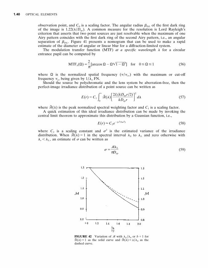
FIGURE 42 Variation of with l L / l S or b 1 1 for 5 ( l ) 5 1 as the solid curve and 5 ( l ) 5 l / l S as the dashed curve .

LENSES 1 .41

where 5 1 . 335 2 0 . 625 b 1 0 . 25 b 2 2 0 . 0465 b 3 with b 5 ( l L / l S ) 2 1 . Should 5 ( l ) 5 l / l L in the spectral interval l S to l L and zero otherwise , which approximates the behavior of a quantum detector , 5 1 . 335 2 0 . 65 b 1 0 . 385 b 2 2 0 . 099 b 3 . The Gaussian estimate residual error is less than a few percent for b 5 0 . 5 and remains useful even as b 5 0 . Figure 42 contains plots of for both cases of 5 ( l ) , where the abscissa is l L / l S .

A useful estimation of the modulation transfer function for this polychromatic lens system is given by

MTF( … ) < e 2 2( π s … ) 2 (60)

where … is the spatial frequency . This approximation overestimates the MTF somewhat at lower spatial frequencies , while being rather a close fit at medium and higher spatial frequencies . The reason for this is that the central portion of the irradiance distribution is closely matched by the Gaussian approximation , while the irradiance estimation beyond several Airy radii begins to degrade , therefore impacting the lower spatial frequencies . Nevertheless , this approximation can provide useful insight into expected performance limits .

1 . 2 2 BIBLIOGRAPHY

Douglas S . Goodman , ‘‘Basic Optical Instruments , ’’ Chap . 4 in Geometrical and Instrumental Optics , Daniel Malacara ed ., Methods of Experimental Physics , 25 , Academic Press , San Diego (1988) .

R . E . Hopkins , ‘‘Geometrical Optics , ’’ Chap . 2 in Geometrical and Instrumental Optics , Daniel Malacara ed ., Methods of Experimental Physics , 25 , Academic Press , San Diego (1988) .

R . E . Hopkins , ‘‘The Components in the Basic Optical Systems , ’’ Chap . 3 in Geometrical and Instrumental Optics , Daniel Malacara ed ., Methods of Experimental Physics , 25 , Academic Press , San Diego (1988) .

R . Barry Johnson and C . Feng , ‘‘A History of IR Lens Designs , ’’ SPIE Critical Reviews CR37 , 3 – 18 (1991) .

Rudolf Kingslake , A History of the Photographic Lens , Academic Press , San Diego (1989) . Rudolf Kingslake , Lens Design Fundamentals , Academic Press , New York (1978) . Rudolf Kingslake , Optical System Design , Academic Press , New York (1983) . Rudolf Kingslake , Optics in Photography , SPIE Press , Bellingham , (1992) . Rudolf Kingslake , ‘‘Basic Geometrical Optics , ’’ Chap . 6 in Applied Optics and Optical Engineering , 1 ,

Academic Press , New York (1965) . Milton Laikin , Lens Design , Marcel Dekker , New York (1991) . MIL-HDBK-141 , Optical Design , Defense Supply Agency , Washington (1962) . Warren J . Smith , Modern Lens Design , A Resource Manual , McGraw-Hill , New York (1992) . Warren J . Smith , Modern Optical Engineering , second edition , McGraw-Hill , New York (1990) .

Chapter 1 - Handbook of Optics -...

Documents

Transcript of Chapter 1 - Handbook of Optics -...