Chapter 2

Organizing Data

Understanding Basic Statistics Fifth Edition

By Brase and Brase Prepared by Jon Booze

2 | 2Copyright © Cengage Learning. All rights reserved.

Frequency Tables

• A frequency table– organizes quantitative data.– partitions data into classes (intervals).– shows how many data values are in each

class.

Test Score Number of Students

61-70 4

71-80 8

81-90 15

91-100 7

2 | 3Copyright © Cengage Learning. All rights reserved.

Data Classes and Class Frequency• Class: an interval of values.

– Example: 61 x 70

• Frequency: the number of data values that fall within a class.

– “Four data fall within the class 61 x 70”.

• Relative Frequency: the proportion of data values that fall within a class.

– “0.1176 of the data fall within the class 61 x 70”.

2 | 4Copyright © Cengage Learning. All rights reserved.

Structure of a Data ClassA “data class” is basically an interval on a number

line.

It has:• A lower limit a and an upper limit b.• A width.• A lower boundary and an upper boundary (integer data).• A midpoint.

2 | 5Copyright © Cengage Learning. All rights reserved.

Structure of a Data ClassA “data class” is basically an interval on a number

line.

If a = 60 and b = 69 for integer data, what is the value of the lower boundary?

a). 60 b). 59.5

c). 9 d). 64.5

2 | 6Copyright © Cengage Learning. All rights reserved.

Structure of a Data ClassA “data class” is basically an interval on a number

line.

If a = 60 and b = 69 for integer data, what is the value of the lower boundary?

a). 60 b). 59.5

c). 9 d). 64.5

2 | 7Copyright © Cengage Learning. All rights reserved.

Constructing Data Classes• Find the class width.

–

– Increase the computed value to the next higher whole number.

• Find the class limits. – The lower limit of the “leftmost” class is set

equal to the smallest value in the data set.

Largest data value – smallest data valueDesired number of classes

2 | 8Copyright © Cengage Learning. All rights reserved.

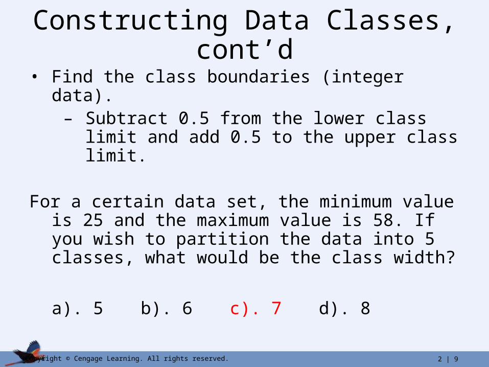
Constructing Data Classes, cont’d

• Find the class boundaries (integer data).– Subtract 0.5 from the lower class limit and

add 0.5 to the upper class limit.

For a certain data set, the minimum value is 25 and the maximum value is 58. If you wish to partition the data into 5 classes, what would be the class width?

a). 5 b). 6 c). 7 d). 8

2 | 9Copyright © Cengage Learning. All rights reserved.

Constructing Data Classes, cont’d

• Find the class boundaries (integer data).– Subtract 0.5 from the lower class limit and

add 0.5 to the upper class limit.

For a certain data set, the minimum value is 25 and the maximum value is 58. If you wish to partition the data into 5 classes, what would be the class width?

a). 5 b). 6 c). 7 d). 8

2 | 10Copyright © Cengage Learning. All rights reserved.

Building a Frequency Table• Find the class width, class limits, and class

boundaries of the data.• Use Tally marks to count the data in each class.• Record the frequencies (and relative

frequencies if desired) on the table.

2 | 11Copyright © Cengage Learning. All rights reserved.

Histograms• Histogram – graphical summary of a frequency

table.• Uses bars to plot the data classes versus the

class frequencies.

• Place class boundaries on horizontal axis. Place frequencies (or relative frequencies) on vertical axis.

• For each class, draw a bar with height equal to the class frequency.

2 | 12Copyright © Cengage Learning. All rights reserved.

Making a Histogram

2 | 13Copyright © Cengage Learning. All rights reserved.

Distribution Shapes

Symmetric Uniform

Skewed Left (Negative)

Skewed Right (Positive)

Bimodal

2 | 14Copyright © Cengage Learning. All rights reserved.

Critical Thinking

• A bimodal distribution shape might indicate that the data are from two different populations.

• Outliers – data values that are very different from other values in the data set.

• Outliers may indicate data recording errors.

2 | 15Copyright © Cengage Learning. All rights reserved.

Graphical Displays…

• … represent the data.

• … induce the viewer to think about the substance of the graphic.

• …should avoid distorting the message of the data.

2 | 16Copyright © Cengage Learning. All rights reserved.

Bar Graphs

• Used for qualitative or quantitative data.

• Can be vertical or horizontal.

• Bars are uniformly spaced and have equal widths.

• Length/height of bars indicate counts or percentages of the variable.

• “Good practice” requires including titles and units and labeling axes.

2 | 17Copyright © Cengage Learning. All rights reserved.

Bar Graphs

Example:

2 | 18Copyright © Cengage Learning. All rights reserved.

Pareto Charts

• A bar chart with two specific features:

– Heights of bars represent frequencies.

– Bars are vertical and are ordered from tallest to shortest.

2 | 19Copyright © Cengage Learning. All rights reserved.

Circle Graphs/Pie Charts• Used for qualitative data

• Wedges of the circle represent proportions of the data that share a common characteristic.

• “Good practice” requires including a title and either wedge labels or legend.

2 | 20Copyright © Cengage Learning. All rights reserved.

Critical Thinking – which type of graph to use?

• Bar graphs are useful for quantitative or qualitative data.

• Pareto charts identify the frequency in decreasing order.

• Circle graphs display how a total is dispersed into several categories.

• Time-series graphs display how data change over time.

2 | 21Copyright © Cengage Learning. All rights reserved.

Time-Series• Shows data measurements in chronological

order.

• Data are plotted in order of occurrence at regular intervals over a period of time.

2 | 22Copyright © Cengage Learning. All rights reserved.

Stem and Leaf Plots• Displays the distribution of the data while

maintaining the actual data values.

• Each data value is split into a stem and a leaf.

2 | 23Copyright © Cengage Learning. All rights reserved.

Stem and Leaf Plot Construction

2 | 24Copyright © Cengage Learning. All rights reserved.

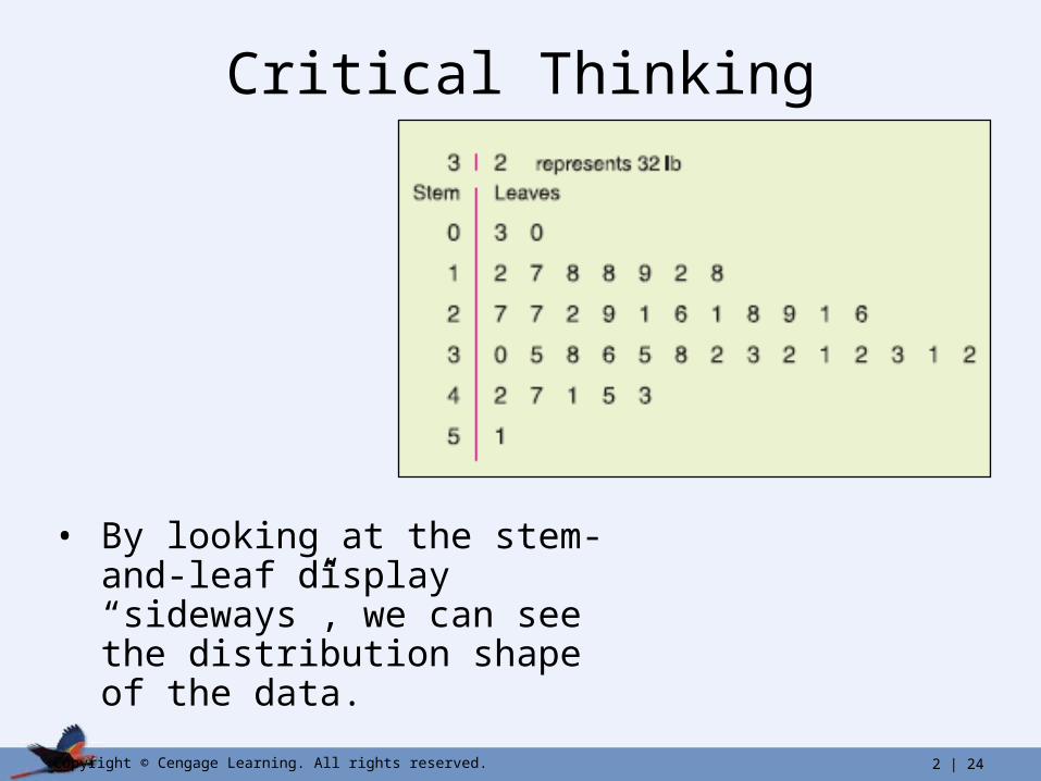
Critical Thinking

• By looking at the stem-and-leaf display “sideways”, we can see the distribution shape of the data.

2 | 25Copyright © Cengage Learning. All rights reserved.

Critical Thinking

• Large gaps between stems containing leaves, especially at the top or bottom, suggest the existence of outliers.

• Watch the outliers – are they data errors or simply unusual data values?