Chapter 2

Lagrangian mechanics

2.1 From Newton II to the Lagrangian

In the coming sections we will introduce both the notion of a Lagrangian as well asthe principle of least action. This will be an equivalent, but much more powerful,formulation of Newtonian mechanics than what can be achieved starting from Newton’ssecond law. However, to introduce this new way of thinking, we will in this section givea short argument why the Lagrangian is a “natural” object to study.

Consider now a single particle at position x in a potential V (x, t). The kinetic energyof this particle is T = 1

2mx2. The equation of motion for this particle is

mx = − ∂

∂xV (x, t). (2.1)

What we ultimately seek, is a way to generate this equation of motion from a simplerobject. Playing around with this equation we note that we can write mx = d

dt∂∂xT . We

may thus rewrite (2.1) asd

dt

∂

∂xT (x) = − ∂

∂xV (x, t).

Note that since T does not depend on x and V does not depend on x we can rewritethe equation further as (

d

dt

∂

∂x− ∂

∂x

)(T − V ) = 0. (2.2)

This funny looking equation will be the starting point for this course. The differenceL = T − V we will call the Lagrangian, and the differential operator d

dt∂∂x− ∂

∂xwill be

obtained from the principle of least action. We will find that (2.2) is more general thanmeets the eye. Especially, it will look the same irrespective of the coordinate systemthat we are working in. The same thing can not be said for Newton II, which becomesmuch more complicated when the coordinate system is not the Cartesian one.

2.2 The principle of least action

The starting point for the reformulation of classical mechanics is the principle of leastaction, which may be somewhat flippantly paraphrased as “The world is lazy”, or in

4

the more flowery words of Pierre Louis Maupertuis (1744), Nature is thrifty in all itsactions :

The laws of movement and of rest deduced from this principle being preciselythe same as those observed in nature, we can admire the application of it toall phenomena. The movement of animals, the vegetative growth of plants. . . are only its consequences; and the spectacle of the universe becomes somuch the grander, so much more beautiful, the worthier of its Author, whenone knows that a small number of laws, most wisely established, suffice forall movements.

This very general formulation does not in itself have any predictive power, but theidea that nature’s “thrift” could be used to derive laws of motion had already beensuccessfully applied in optics for a long time:

Fermat’s principleThe path take between two points by a ray of light is the path that can be traversedin the least time.

This principle was first formulated by Ibn al-Haytham (aka Alhacen) in his Book ofOptics from 1021, which formed one of the main foundations of geometric optics andthe scientific method in general. He proved that it led to the law of reflection. It wasrestated by Pierre de Fermat in 1662, who also derived Snell’s law of refraction fromthis principle.

2.2.1 Hamilton’s principle

In mechanics the proper mathematical formulation of Maupertuis’ principle is due toWilliam Rowan Hamilton1, building on earlier work by Joseph Louis Lagrange.

We will denote the kinetic and potential energy of a particle, or of a mechanical systemin general, as

T = kinetic energy

V = potential energy

T usually depends on the velocities vi = dxidt≡ xi T = T (xi

V usually depends on the positions xi V = V (xi)but may also depend explicitly on time t V = V (xi, t)(for example with time-varying extermal forces).

xi and xi here denote all the coordinates and their time derivatives. So for example wehave

xi → x for a single particle in one dimension

xi → {x, y, z} for a particle in three dimensions

xi → {x1, y1, z1, x2, y2, z2, . . . , xN , yN , zN} for N particles in three dimensions

1On a General Method in Dynamics, Phil. Trans. Roy. Soc. (1834) 247; (1835) 95.

5

We now define the lagrangian L as the difference between kinetic and potential energy,

L(xi, xi, t) = T − V . (2.3)

Note that L will be a function of the coordinates xi, the velocities xi, and the time t,although in many cases there is no explicit time dependence; ie, if we know the positionsand velocities of all the particles we know the lagrangian.

A particular path is given by specifying the coordinates xi as a function of time, xi =xi(t). (Note that if xi(t) is known, its derivative xi(t) is also known.) For a given path,the action S is defined as

S[x] ≡t2∫t1

L(x(t), x(t), t)dt . (2.4)

We are now in a position to formulate Hamilton’s principle of least action.

The principle of least action:

The physical path a system will take between two points in a certain time interval isthe one that gives the smallest action S.

Comments:

1. The potential energy V is defined only for conservative forces, so the action as itis written here is defined only for conservative forces. It is possible to generalisethis to certain non-conservative forces and obtain the correct equations of motion(we will see examples of this later). However, all microscopic (fundamental) forcesare conservative.

2. The action S is a “function of a function” since it depends on the function(s) xi(t).We call this a functional, and denote it by putting the function argument in squarebrackets, S = S[x].

2.3 The Euler–Lagrange equations

x1(t1)

x2(t2)

x(t)

x’(t)

What does ‘the path that gives the smallest action’ actuallymean, and how can we find it? To work this out, let usconsider a path x(t) and another path x′(t) = x(t) + αh(t),where h(t) is some arbitrary smooth function of t, and α isa parameter that we will vary.

6

Since we are looking for the path the system will take be-tween two specific points in a specific time interval, theendpoints of the two paths must be the same. We thereforehave

x(t1) = x′(t1) = x1 ; x(t2) = x′(t2) = x2 ⇐⇒ h(t1) = h(t2) = 0 . (2.5)

We can now write S[x+ αh] = S(α), and treat it as a function of the parameter α. Fora given h(t), the minimum of S will occur when dS

dα= 0.

This allows us to restate the principle of least action:For any smooth hi(t) with hi(t1) = hi(t2) = 0, the physical path xi(t) is such that

d

dαS[x+ αh] =

d

dα

t2∫t1

L(xi + αhi, xi + αhi, t)dt = 0 . (2.6)

We often use the shorthands αh = δx and S[x+ δx]− S[x] = δS = the variation of S,and call δS

δxthe functional derivative of S. The principle of least action is then often

written as

δS = 0 orδS

δx= 0 ⇐⇒ d

dαS[x+ αh] = 0 for any h(t) . (2.7)

Let us now calculate the variation δS. For a single particle in one dimension, we have

d

dαS[x+ αh] =

d

dα

∫ t2

t1

L(x+ αh, x+ αh, t)dt (2.8)

=

∫ t2

t1

(∂L

∂xh+

∂L

∂xh

)dt (2.9)

=

∫ t2

t1

∂L

∂xh dt+

[∂L

∂xh

]t=t2t=t1

−∫ t2

t1

(d

dt

∂L

∂x

)h dt (2.10)

=

∫ t2

t1

(∂L

∂x− d

dt

∂L

∂x

)h(t)dt . (2.11)

In the first step we used that L is a function of the three variables x, x, t, but t does notdepend on α. We can then use the chain rule for a function of two variables,

d

dαf(x, y) =

∂f

∂x

dx

dα+∂f

∂y

dy

dα.

In the second step we used integration by parts,∫uvdt = uv −

∫uvdt with u =

∂L

∂x, v = h .

In the final step the boundary term vanishes since h(t1) = h(t2) = 0.

But h(t) is a completely arbitrary smooth function, and we must have δS = 0 for anyh(t). This is only possible if the term within the brackets in (2.11) is 0 for all t, ie

7

d

dt

∂L

∂x− ∂L

∂x= 0 The Euler–Lagrange equation (2.12)

If we have N coordinates xi, the derivation proceeds following the same steps. Usingthe chain rule for a function of 2N variables, we find

d

dαL(x1 + αh1, x2 + αh2, . . . , xN + αhN , x1 + αh1, x2 + αh2, . . . , xN + αhN)

=∂L

∂x1h1 +

∂L

∂x2h2 + · · ·+ ∂L

∂xNhN +

∂L

∂x1h1 +

∂L

∂x2h2 + · · ·+ ∂L

∂xNhN

=N∑i=1

(∂L

∂xihi +

∂L

∂xihi

). (2.13)

Using integration by parts on the second term (for each i) gives us

d

dαS[x+ αh] =

N∑i=1

∫ t2

t1

( ∂L∂xi− d

dt

∂L

∂xi

)hi(t)dt = 0 . (2.14)

Since all the hi are independent, arbitrary functions, the expression within the bracketsmust vanish for each i:

d

dt

∂L

∂xi− ∂L

∂xi= 0 for all i = 1, . . . , N . (2.15)

Example 2.1 Particle in a potential

The kinetic energy of a single particle is

T =1

2mv2 =

1

2m(v2x + v2y + v2z) =

1

2m(x2 + y2 + z2) . (2.16)

We take an arbitrary potential energy V = V (x, y, z, t).

The Euler–Lagrange equations are

d

dt

∂L

∂x− ∂L

∂x= 0 ;

d

dt

∂L

∂y− ∂L

∂y= 0 ;

d

dt

∂L

∂z− ∂L

∂z= 0 . (2.17)

We find

∂L

∂x= mx ;

∂L

∂x= −∂V

∂x(2.18)

=⇒ d

dt

∂L

∂x− ∂L

∂x= mx+

∂V

∂x= 0 ⇐⇒ mx = −∂V

∂x. (2.19)

Likewise, we get

my = −∂V∂y

, mz = −∂V∂z

or

m~a = m~r = −∇V = ~F = Newton’s 2nd law!

So the Euler–Lagrange equations are exactly equivalent to Newton’s laws.

8

Example 2.2 The shortest path between two points

In deriving the Euler–Lagrange equations we did not make any use of the definitionof L: it could be any function of x, x and t. Therefore, the EL equations give thestationary points for any functional of the path between two points — for example,the length of the path!

Consider a curve y = y(x) between two points (x1, y1) and (x2, y2). The length dsof an infinitesimal segment (dx, dy) of this curve is given by Pythagoras:

ds2 = dx2 + dy2 = dx2 + (y′(x)dx)2 = (1 + y′(x)2)dx2 (2.20)

=⇒ ds =√

1 + y′(x)2dx . (2.21)

If, to make life simpler for ourselves, we assume that x is monotonically increasingalong the curve, we find that the total length of the curve is

S =

∫ x2

x1

√1 + y′(x)2dx =

∫ x2

x1

L(y(x), y′(x), x)dx with L =

√1 + y′2 . (2.22)

This looks like what we had before, but with t→ x;x(t)→ y(x); x(t)→ y′(x).

The Euler–Lagrange equation becomes

d

dt

∂L

∂y′− ∂L

∂y= 0 . (2.23)

We see immediately that ∂L/∂y = 0. To find ∂L/∂y′ we use the chain rule,

∂L

∂y′=dL

du

∂u

∂y′with u = 1 + y′

2; L =

√u

=⇒ ∂L

∂y′=

1

2√

1 + y′2· 2y′ = y′√

1 + y′2.

To find ddx

∂L∂y′

we use the product rule and the chain rule:

∂L

∂y′= vw with v = y′ , w =

1√1 + y′2

= u−1/2 (2.24)

=⇒ d

dx

∂L

∂y′=dv

dxw + v

dw

du

du

dx=dy′

dxw + y′

dw

du

du

dy′dy′

dx

= y′′1√

1 + y′2+ y′ ·

(− 1

2u−3/2

)· 2y′ · y′′

= y′′( 1√

1 + y′2− y′2

(1 + y′2)3/2

)=

y′′√1 + y′2

(1− y′2

1 + y′2

)=

y′′√1 + y′2

1

1 + y′2.

(2.25)

Sod

dx

∂L

∂y′= 0 =⇒ y′′(x) = 0 =⇒ y(x) = Ax+B . (2.26)

This describes a straight line, so we have shown that the shortest path between twopoints is a straight line!

9

So what is the point?

1. The equations are often easier : We get rid of complicated vectors and forces, andderive everything from scalars (energy).

2. It is easier to generalise to systems with constraints.

3. We can choose whichever coordinates we want.

4. The lagrangian formalism can be generalised to quantum mechanics (in the Feyn-man formulation: all paths are possible, but weighted by the action) and fieldtheory (with infinitely many degrees of freedom).

We will look at points 2 and 3 next.

2.4 Generalised coordinates

It is often advantageous to change variables from the cartesian coordinates {xi, yi, zi}for each particle i = 1, . . . , N to some other variables {qj}, j = 1, . . . , n. These are calledgeneralised coordinates.

Consider for example a system of N particles. We need 3N independent coordinates todescribe the system completely: we say that there are 3N degrees of freedom.

Now, imagine that there is a constraint relating the 3N coordinates, for example:

1. Two particles are tied together with a rod of length L, so that

(x1 − x2)2 + (y1 − y2)2 + (z1 − z2)2 = L2 . (2.27)

2. The N particles are all moving on the surface of a sphere, ie

x2i + y2i + z2i = R2 ∀i = 1, . . . , N . (2.28)

3. A ball in a squash court, x ≥ 0, z ≥ 0.

The first two of these can be described by M equations of the form

fj(~x1, . . . , ~xN , t) = 0 , j = 1, . . . ,M . (2.29)

Such constraints are called holonomic (or integrable) constraints, and we will focus onlyon such constraints in the following. With such constraint equations, the coordinatesxi, yi, zi are no longer independent. Instead we have

M relations =⇒ n = 3N −M real degrees of freedom.

By choosing n suitable generalised coordinates to describe these degrees of freedom, weachieve two things:

10

• We eliminate the forces of constraints which are required in the newtonian formu-lation. No net work is done by these forces, so they can safely be eliminated.

• The Euler–Lagrange equations look exactly the same in the new coordinates, sothe problem is no more difficult (and probably easier) than the original one.

In the first example above, the constraint (2.27) reduces the number of degrees of freedomfrom 6 to 5. The 5 coordinates can for example be chosen to be the centre of masscoordinatesX, Y, Z for the two particles, and two angles θ, φ that describe the orientationof the rod.2

In the second example, each particle is described by 2 instead of 3 coordinates. Thesecan be chosen to be the ‘latitude’ θ and ‘longitude’ φ of each particle (corresponding tospherical coordinates, see Sec. 2.4.1).

Example 2.3 Simple pendulum

Consider a simple pendulum with length `, mass m in a constant gravitational fieldg (see Fig. 2.1).

rAAAAAAAAAAA|

`

m

. ................ ................................................

θ

Figure 2.1: A simple pen-dulum

Here it is convenient to choose the angle θ as our coor-dinate. The x (horizontal) and z (vertical) coordinatesand their time derivatives can be written in terms of θ as

x = ` sin θ x = `θ cos θ , (2.30)

z = −` cos θ z = `θ sin θ . (2.31)

The kinetic energy is

T =1

2m~v2 =

1

2m(x2 + z2)

=1

2m`2θ6(cos2 θ + sin2 θ) =

1

2m`2θ2 . (2.32)

The potential energy is

V = mgz = −mg` cos θ . (2.33)

The lagrangian therefore becomes

L = T − V =1

2m`2θ2 +mg` cos θ . (2.34)

The Euler–Lagrange equation is

∂L

∂θ=

d

dt

∂L

∂θ=⇒ −mg` sin θ =

d

dt

(m`2θ

)(2.35)

=⇒ θ = −g`

sin θ . (2.36)

This is the equation of motion for the pendulum.

2In Chapter 5 we will look more at how these angles can be chosen.

11

Once we have found the equation of motion for θ, and the solution to this equation, wecan go back and calculate x and z as functions of time. However, in the example of thesimple pendulum, we are not usually interested in this.

We note that the mass m does not appear in the equation of motion. We could haveseen this already by inspecting the lagrangian: the EL equations are unchanged if thelagrangian is multiplied by an overall constant α, L→ αL. In this case, since the massjust enters as an overall factor in the lagrangian, the EL equation will not depend onthe mass.

Solutions to the equations of motion?

Now we have found the equation of motion for the simple pendulum, and we may wantto know the solutions to this equation, ie what the actual motion of the pendulum is fordifferent initial conditions. It is actually possible to integrate the equation (2.36) andwrite down a solution, but this involves elliptic integrals and lots of other complicatedmaths, and will not help us to understand the physical system. It will be more useful tofind numerical solutions, and in Computational Physics MP354 we will learn how thiscan be done.

What we can do to understand the system better, is

• look at the general types of solutions we may have. We will do this when wediscuss conservation of energy;

• consider limiting cases such as small oscillations. This is what we will do now.

If θ is small, we may approximate sin θ with the first term in its power expansion (Taylorexpansion),

sin θ = θ − 1

3!θ2 +

1

5!θ5 + · · · ≈ θ . (2.37)

In that case (2.36) simplifies to

θ = −g`θ . (2.38)

We recognise this as the equation for a simple harmonic oscillator, x + ω2x = 0, withx → θ, ω2 → g/`. We therefore see that for small oscillations, the simple pendulumbehaves as a simple harmonic oscillator with frequency ωs =

√g/`, ie the frequency is

inversely proportional to the square root of the length of the pendulum (and independentof the mass).

12

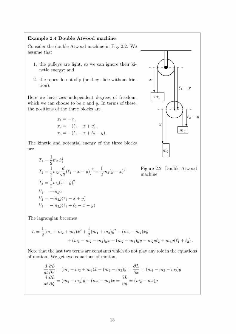
Example 2.4 Double Atwood machine

m1

x

?

......................................................................................................................................................................................

.............

.............

.......................... ............. ............. ............. ............. ............. ............. ............. ............. .............

.................................................................

x

`1 − x

? ......................................................................................................................................................................................

.............

.............

.......................... ............. ............. ............. ............. ............. ............. ............. ............. .............

.................................................................

s

?

y

m2

?

`2 − y

m3

Figure 2.2: Double Atwoodmachine

Consider the double Atwood machine in Fig. 2.2. Weassume that

1. the pulleys are light, so we can ignore their ki-netic energy; and

2. the ropes do not slip (or they slide without fric-tion).

Here we have two independent degrees of freedom,which we can choose to be x and y. In terms of these,the positions of the three blocks are

x1 = −x ,x2 = −(`1 − x+ y) ,

x3 = −(`1 − x+ `2 − y) .

The kinetic and potential energy of the three blocksare

T1 =1

2m1x

21

T2 =1

2m2

[ ddt

(`1 − x− y)]2

=1

2m2(y − x)2

T3 =1

2m3(x+ y)2

V1 = −mgxV2 = −m2g(`1 − x+ y)

V3 = −m2g(`1 + `2 − x− y)

The lagrangian becomes

L =1

2(m1 +m2 +m3)x

2 +1

2(m1 +m2)y

2 + (m3 −m2)xy

+ (m1 −m2 −m3)gx+ (m2 −m3)gy +m2g`2 +m3g(`1 + `2) .

Note that the last two terms are constants which do not play any role in the equationsof motion. We get two equations of motion:

d

dt

∂L

∂x= (m1 +m2 +m3)x+ (m3 −m2)y =

∂L

∂x= (m1 −m2 −m3)g

d

dt

∂L

∂y= (m2 +m3)y + (m3 −m2)x =

∂L

∂y= (m2 −m3)g

13

Example 2.5 Pendulum with rotating support

.................

..................

..................

..................

.................

................

................

...................................

............................................................................................................................

.................

................

................

.................

..................

..................

..................

........

........

.

........

........

.

..................

..................

..................

.................

................

................

.................

.................. .................. .................. ................. ................. ....................................

...................................

................

................

.................

..................

..................

..................

.................s����a

............................. ωt

................

..............

..........................................................

ω

sCCCCCCCCCCCCCCCCCC

`

|m

. ..................... ...................... ......................

θ

Figure 2.3: Pendulum withrotating support.

Consider a pendulum mounted on the edge of a discwith radius a, rotating with constant angular velocityω (see Fig. 2.3). If the support point is in the hori-zontal position at t = 0, the angular position of thesupport point at time t is φ = ωt, and the cartesiancoordinates of the bob at time t are

x = a cosωt+ ` sin θ

z = a sinωt− ` cos θ

giving the velocities

x = −aω sinωt+ `θ cos θ

z = aω cosωt+ `θ sin θ

This gives us the lagrangian

L = T − V =1

2m(x2 + z2)−mgz

=m

2

(a2ω2 + `2θ2 + 2aω`θ sin(θ − ωt)

)−mg

(a sinωt− ` cos θ

)This system has only one degree of freedom θ, but the lagrangian depends explicitlyon time because of the rotation of the support point. The Euler–Lagrange equationis

d

dt

∂L

∂θ=

d

dt

(m`2θ +maω` sin(θ − ωt)

)= m`2θ +maω`(θ − ω) cos(θ − ωt)

=∂L

∂θ= maω`θ cos(θ − ωt) +mg` sin θ

=⇒ `θ − aω2 cos(θ − ωt) = −g sin θ =⇒ θ =aω2

`cos(θ − ωt)− g

`sin θ

Finding the equation of motion for this system becomes a bit complicated, but it isstill far simpler than it would have been to compute the forces at each point and useNewton’s second law.

We can check that our result is sensible by seeing what happens if there is no rotation,ie ω = 0. In this case the system reduces to the simple pendulum, and the equationof motion should be the same. We can immediately see that this is the case.

It is worth noting that the potential energy contains a time-dependent termmga sinωt, which one naively would think should contribute to the dynamics ofthe system — however, it plays no role since it does not contain the coordinate θ.There is also a constant term ma2ω2/2 in the kinetic energy which plays no role.NB: If you removed a sinωt from the definition of z, you would for consistency alsoneed to remove aω cosωt from z, and this will change the dynamics.

14

2.4.1 Polar and spherical coordinates

When we have rotational motion, or a system with rotational (or spherical) symmetry,it is very often most convenient to use polar coordinates (in 2 dimensions) or sphericalcoordinates (in 3 dimensions). The definition of these coordinates are given in Fig. 2.4.Since we will be using them often, we need to know what the kinetic energy of a particleis in terms of these coordinates.

-

6

����

���

��*

y

x

rθ

.

.................

..................

..................

..................

-

6

��

���

��

����������

SS

. .............. ............... ............... ...............

.............

................. ............... ............... ............... ............... ...............

...............

θ

φ

r

z

x

y

Figure 2.4: Plane polar coordinates (r, θ) (left) and spherical coordinates (r, θ, φ) (right).

Polar coordinates

The relation between cartesian and polar coordinates is given by

x = r cos θ =⇒ x = r cos θ − rθ sin θ (2.39)

y = r sin θ =⇒ y = r sin θ + rθ cos θ (2.40)

This gives for the kinetic energy,

T =1

2m(x2 + y2)

=m

2(r2 cos2 θ + r2θ2 sin2 θ − 2rrθ cos θ sin θ + r2 sin2 θ + r2θ2 cos2 θ + 2rrθ cos θ sin θ)

=m

2(r2 + r2θ2) . (2.41)

15

Spherical coordinates

The relation between cartesian and spherical coordinates is given by

x = r sin θ cosφ =⇒ x = r sin θ cosφ+ rθ cos θ cosφ− rφ sin θ sinφ (2.42)

y = r sin θ sinφ =⇒ y = r sin θ sinφ+ rθ cos θ sinφ+ rφ sin θ cosφ (2.43)

z = r cos θ =⇒ z = r cos θ − rθ sin θ (2.44)

Using this we find that

T =1

2m(x2 + y2 + z2) =

1

2m(r2 + r2θ2 + r2φ2 sin2 θ) . (2.45)

The complete derivation is left as an exercise.

2.5 Lagrange multipliers [Optional]

Using the constraint equations to reduce the number of coordinates is usually the moststraightforward way of handling constraints. But it is not always practical:

• It may not be straightforward to solve the constraint equations.

• The constraint equations may involve velocities.

• The constraint equations may be expressed as differential rather than algebraicequations.

• We may want to know the forces of constraint (for example, to find out when theybecome too large or too small to physically constrain the system).

2.5.1 Velocity constraints and differential constraints

A constraint relation of the form

gα(x, x, t) = 0 , x = {x1, . . . , xN} (2.46)

involving velocities xi, can in general not be integrated to yield relations between coor-dinates. However, consider the equation∑

i

Ai(x, t)xi +B(x, t) = 0 , . (2.47)

If we can write

Ai =∂f

∂xiB =

∂f

∂twith f = f(x, t) , (2.48)

then (2.47) is equivalent to an algebraic relation among the coordinates xi:∑i

∂f

∂xi

dxidt

+∂f

∂t=df

dt= 0 (2.49)

⇐⇒ f(x, t)− C = 0 . (2.50)

This is an example of a differential constraint∑i

∂fj∂qi

dqi +∂fj∂tdt = 0 . (2.51)

16

2.5.2 Lagrange undetermined multipliers

Assume now that we are keeping our original coordinates qi (whatever they are) andwrite the constraint equations on the differential form (2.51). We can now try to rederivethe Euler–Lagrange equations.

Consider a variation qαi (t) = qi(t) + αhi(t). We find, as before,

dS

dα=

d

dα

∫ t2

t1

L(qαi , qαi , t)dt =

∫ t2

t1

N∑i=1

(∂L∂qi− d

dt

∂L

∂qi

)hidt = 0 . (2.52)

However, the functions hi are no longer independent, since the qαi must satisfy theequations (2.51). In particular, we must have∑

i

∂fj∂qi

dqαidα

=∑i

∂fj∂qi

hi = 0 . (2.53)

Note that the second term in (2.51) does not contribute, since dt/dα = 0 as t is notvaried.

If we have m constraint equations, we can use them to eliminate m of the functions hi:

∂f1∂qN

hN(t) = −N−1∑i=1

∂f1∂qi

hi(t) ⇐⇒ hN(t) = −∑

i = 1N−1∂f1/∂qi∂f1/∂qN

hi(t) (2.54)

∂f2∂qN−1

hN−1(t) = −N−2∑i=1

∂f2∂qi

hi(t)−∂f2∂qN

hN(t)

= −N−2∑i=1

∂f2∂qi

hi(t)−∂f2/∂qN∂f1/∂qN

N−2∑i=1

∂f1∂qi

hi(t)−∂f2/∂qN∂f1/∂qN

∂f1∂qN−1

hN−1(t)

(2.55)

. . . etc.

This becomes messy and not very illuminating in general, so let us consider just thecase with m = 1, N = 3. Eq. (2.54) then becomes

h3 = −∂f/∂q1∂f/∂q3

h1 −∂f/∂q2∂f/∂q3

h2 (2.56)

and (2.52) becomes∫ t2

t1

{( ∂L∂q1− d

dt

∂L

∂q1

)h1 +

( ∂L∂q2− d

dt

∂L

∂q2

)h2 +

( ∂L∂q3− d

dt

∂L

∂q3

)h3

}dt = 0 (2.57)

⇐⇒∫ t2

t1

{[(∂L

∂q1− d

dt

∂L

∂q1

)− ∂f/∂q1∂f/∂q3

(∂L

∂q3− d

dt

∂L

∂q3

)]h1

+[(∂L

∂q2− d

dt

∂L

∂q2

)− ∂f/∂q2∂f/∂q3

(∂L

∂q3− d

dt

∂L

∂q3

)]h2

}dt = 0

(2.58)

Since h1 and h2 are now both arbitrary functions, the terms inside the square bracketsmust both be zero. So we have

(∂L

∂q1− d

dt

∂L

∂q1

)( ∂f∂q1

)−1= (

∂L

∂q3− d

dt

∂L

∂q3

)( ∂f∂q3

)−1(∂L

∂q2− d

dt

∂L

∂q2

)( ∂f∂q2

)−1= (

∂L

∂q3− d

dt

∂L

∂q3

)( ∂f∂q3

)−1 at all t . (2.59)

17

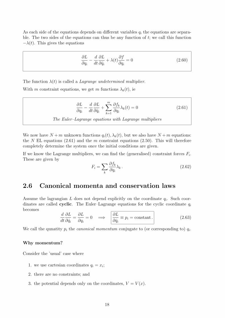
As each side of the equations depends on different variables qi the equations are separa-ble. The two sides of the equations can thus be any function of t; we call this function−λ(t). This gives the equations

∂L

∂qi− d

dt

∂L

∂qi+ λ(t)

∂f

∂qi= 0 (2.60)

The function λ(t) is called a Lagrange undetermined multiplier.

With m constraint equations, we get m functions λk(t), ie

∂L

∂qi− d

dt

∂L

∂qi+

m∑k=1

∂fk∂qi

λk(t) = 0 (2.61)

The Euler–Lagrange equations with Lagrange multipliers

We now have N +m unknown functions qi(t), λk(t), but we also have N +m equations:the N EL equations (2.61) and the m constraint equations (2.50). This will thereforecompletely determine the system once the initial conditions are given.

If we know the Lagrange multipliers, we can find the (generalised) constraint forces Fi.These are given by

Fi =∑k

∂fk∂qi

λk . (2.62)

2.6 Canonical momenta and conservation laws

Assume the lagrangian L does not depend explicitly on the coordinate qi. Such coor-dinates are called cyclic. The Euler–Lagrange equations for the cyclic coordinate qibecomes

d

dt

∂L

∂qi=∂L

∂qi= 0 =⇒ ∂L

∂qi≡ pi = constant . (2.63)

We call the qunatity pi the canonical momentum conjugate to (or corresponding to) qi.

Why momentum?

Consider the ’usual’ case where

1. we use cartesian coordinates qi = xi;

2. there are no constraints; and

3. the potential depends only on the coordinates, V = V (x).

18

In this case we have

L = T − V =1

2m∑j

x2j − V (x) =⇒ ∂L

∂xi= mxi = pi = ordinary momentum.

So we have found the law of conservation of momentum pi if the potential V does notdepend on the coordinate xi — ie, if the system is translationally invariant in the i-direction. Note that if V does not depend on xi this implies that there are no net forcesin the i-direction.

We may in a similar way demonstrate conservation of total momentum for a system ofn particles if the potential energy does not depend on the centre of mass coordinate.But the concept of canonical momenta is much more general and powerful than this,and can be used to derive a whole host of other conservation laws. One of the mostimportant is angular momentum, which we will look at next.

2.6.1 Angular momentum

Consider a one-particle rotationally symmetric 2-dimensional system, and let us usepolar coordinates (r, θ) to describe the parrticle. Rotational symmetry then means thatthe potential energy V (r, θ) = V (r), independent of the angle θ. The lagrangian is then

L = T − V =1

2m(r2 + r2θ2)− V (r) . (2.64)

We see that θ is a cyclic coordinate, and the canonical momentum pθ is therefore con-served. What is this canonical momentum?

We straightforwardly find

pθ =∂L

∂θ=

∂

∂θ

(1

2mr2θ2

)= mr2θ . (2.65)

But θ is the same as the angular velocity ω, and we know that the velocity vθ in theangular direction (perpendicular to the radius r) is vθ = rω = rθ, so pθ = r(mvθ). Butthis is exactly equal to the angular momentum of the particle,

Lz = (~r × ~p)z = mrvθ . (2.66)

So the canonical momentum conjugate to the angle θ is the angular momentum, whichis conserved if the system is rotationally symmetric, ie the lagrangian does not dependon θ.

Angular momentum in spherical coordinates

In section 2.4.1 we found that the kinetic energy in spherical coordinates (see Fig. 2.4 is

T =1

2m(r2 + r2θ2 + r2 sin2 θφ2) . (2.45)

The angle φ corresponds to rotations about the z-axis: if a particle rotates about thez-axis, φ changes while r and θ are unchanged. If the potential energy does not depend

19

on φ, we have rotational symmetry about the z-axis, and the canonical momentum pφis conserved. From (2.45) we find

pφ = mr2 sin2 θφ = r(mr sin θφ)(sin θ) . (2.67)

We now want to show that this is equal to the z-component of the angular momentum,Lz = (~r × ~p)z.

6z

�������

. ............ ............ ............ ............θ

...................... .......... ........... ........... ........... ........... ........... ...........

...............................φ ���� r

@@@Rθ

����φ

Figure 2.5: Unit vectors inspherical coordinates.

We can put a coordinate system (r, θ, φ) at the point ~rand decompose the velocity in its (r, θ, φ) components,

~v = vrr + vθθ + vφφ (2.68)

The unit vector r denotes the radial direction, ie thedirection where r changes, while θ, φ are unchanged.Similarly, θ denotes the direction where θ changes whiler, φ are unchanged, and φ denotes the direction where φchanges while r, θ are unchanged. The three vectors areorthogonal, and φ is also orthogonal to z, since motionin the φ-direction does not change z.

The velocity component vφ is the rotational velocity about the z-axis, which again isequal to the distance from the axis times the angular velocity about the axis. Since φ isthe rotational angle about the z-axis, the angular velocity is dφ/dt = φ. The distancefrom the axis is r sin θ, so

vφ = (r sin θ)φ . (2.69)

We can now work out the vector product ~r × m~v in the spherical coordinate system.Since ~r = rr, we need the cross product of r with each unit vector. Using the right-handrule we find

r × θ = φ , r × φ = −θ , r × r = 0 . (2.70)

The z-component of the angular momentum is therefore

Lz = (~r ×m~v)z = mr[r × (vrr + vθθ + vφφ)]z = mr[vθφ− vφθ]z = −mrvφθ · z . (2.71)

6z

������r

HHHHHjθ

. ......... .......... .......... ..........

θ

............................. θ

-sin θ

We now need to work out the scalar product θ · z. Looking at thefigure on the right, we see that since θ is the angle of ~r with thez-axis, and θ is orthogonal to ~r (but still in the z − r plane), theprojection of θ onto the z-axis is θ · z = − sin θ.

Therefore we find that the z-component of the angular momentumis

Lz = (~r ×m~v)z = −mrvφ(− sin θ) = r · (mr sin θφ) · sin θ = pφ .(2.72)

So the canonical momentum pφ is indeed the angular momentum about the z-axis, andit is conserved if we have rotational symmetry about the z-axis.

If we have full spherical symmetry, this means we have rotational symmetry about all 3axes, so by the same argument as above Lx and Ly must also be conserved. Therefore,

for a spherically symmetric system, the angular momentum vector ~L = ~r×~p is conserved.

20

Naıvely one would think that if we have full rotational symmetry, the angle θ shouldalso be irrelevant, and the canonical momentum pθ should also be conserved. However,this is not the case: although the potential energy does not depend on θ, the kineticenergy does, through the term 1

2mr2 sin2 θφ2. This θ-dependence is an artefact of how

we have chosen the coordinate system, but it is an unavoidable artefact: no matterhow we choose our spherical coordinate angles, these coordinates must break the fullspherical symmetry somehow.

We realise the full symmetry by noting that we could have chosen the coordinatesdifferently, eg we could have chosen θ to be the angle with the x-axis and φ to correspondto rotations about the x-axis — which would have led us to find that Lx is conserved.Similarly, if we choose θ to be the angle with the y-axis we will find that Ly is conserved.

2.7 Energy conservation: the hamiltonian

We know that when we have conservative forces, the potential energy depends onlyon positions, and not on time, and the total energy is conserved. We have derivedconservation of linear and angular momentum in lagrangian mechanics, so we may askourselves if we can also derive energy conservation within the same framework?

The answer to this is that not only can we do this, but the energy conservation theoremwe arrive at is more general than the one we already know!

To see how this works, let us take the (total) time derivative of the lagrangian L =L(qi(t), qi(t), t). Using the chain rule and the Euler–Lagrange equations we get

dL

dt=∑i

∂L

∂qiqi +

∑i

∂L

∂qiqi +

∂L

∂t

=∑i

(d

dt

∂L

∂qi

)qi +

∑i

∂L

∂qi

dqidt

+∂L

∂t

=d

dt

∑i

∂L

∂qiqi +

∂L

∂t

(2.73)

⇐⇒ d

dt

(∑i

∂L

∂qiqi − L

)+∂L

∂t≡ dH

dt+∂L

∂t= 0 , (2.74)

where we have defined

H =∑i

∂L

∂qiqi − L =

∑i

piqi − L = the hamiltonian (2.75)

So we find that if the lagrangian does not depend explicitly on time, then the hamiltonianor energy function H is conserved.

To see how this relates to energy conservation as we know it from before, consider asystem of particles in cartesian coordinates, described by the lagrangian

L = T − V =1

2

∑i

miq2i − V (q) .

21

The hamiltonian for this system is

H =∑i

∂L

∂qiqi − L =

∑i

(miqi)qi −[1

2

∑i

miq2i − V (q)

]=

1

2

∑i

miq2i + V (q) = T + V .

(2.76)

So we find that the hamiltonian is equal to the total energy, so conservation of thehamiltonian is the same as energy conservation in this particular (most common) case.

2.7.1 When is H (not) conserved?

We found that H is conserved if L does not depend explicitly on time, ie L(q, q, t) =L(q, q). We would like to understand in what circumstances an explicit time dependencecould appear in the lagrangian. One possibility would be that the potential energydepends explicitly on time in the first place. But there are also other possibilites. Thekinetic energy, written in terms of the original cartesian (or, for that sake, ordinarypolar or spherical coordinates) does not have any explicit time dependence. But timedependence could still appear in either the kinetic or the potential energy when we writeit in terms of generalised coordinates.

To see how this can happen, let us recall why we introduced generalised coordinates inthe first place:

1. Constraints: There are fewer actual degrees of freedom in the system because ofconstraints. We use generalised coordinates to denote the real (relevant) degreesof freedom. An example of this would be the pendulum, where the original x andz coordinates are reduced to the single coordinate θ.

2. Symmetries: There are symmetries in the system which mean that using non-cartesian coordinates may give a simpler description. An example of this wouldbe using polar coordinates for a system with rotational symmetry.

Explicit time-dependence can appear in both those types of cases, leaving us with threepossibilites for how explicit time-dependence could appear in the lagrangian:

1. The potential energy is explicity time-dependent, V = V (x, t). Physically, thismeans that there are external or non-conservative forces, so the energy of thesystem is not conserved.

2. The constraints are time-dependent. An example of that would be Example 5,the pendulum with rotating support. In such cases, external forces are usuallyrequired to maintain the constraint, so the energy of the system is not conserved.

3. We have chosen to use time-dependent transformations xi = fi(q, t) between theold coordinates x and the new coordinates q because this may simplify the de-scription of the system. In this case, the hamiltonian may be not conserved evenif the total energy is conserved.

22

2.7.2 When is H (not) equal to the total energy?

We showed the hamiltonian H is equal to the total energy E when

L = T − V =1

2

∑i

miq2i − V (q) .

More generally, it is the case when

1. V is independent of the velocitiec qi, V = V (q, t), and

2. T is a homegeneous quadratic function of q,

T =∑ij

aij qiqj, .

Proof

TakeL = T = V

∑ij

aij qiqj − V (q, t) (2.77)

We note that we can always arrange it so that aij = aji, since qiqj = qj qi. The canonicalmomenta are

pk =∂L

∂qk=∑i

aikqi +∑j

akj qj = 2∑j

akj qj . (2.78)

The two terms appear because we get a contribution both from the k = j term andfrom the k = i term in the sum. The hamiltonian is then

H =∑i

piqi − L = 2∑ij

aij qiqj −∑ij

aij qiqj + V (q, t) = T + V = E , (2.79)

which completes the proof.

So when does T (not) have this form?

Let us start from cartesian coordinates, where

T =1

2

∑i

mix2i i = 1, . . . , 3N . (2.80)

We now introduce generalised coordinates qj, which are related to the xi via general,time-dependent transformations,

xi = xi(q1, . . . , qm, t) (2.81)

23

Using the chain rule, we find

xi =dxidt

=m∑j=1

∂xi∂qj

qj +∂xi∂t

, (2.82)

x2i =

( m∑j=1

∂xi∂qj

qj +∂xi∂t

)( m∑k=1

∂xi∂qk

qk +∂xi∂t

)

=m∑

j,k=1

∂xi∂qj

qj∂xi∂qk

qk + 2m∑j=1

∂xi∂qj

∂xi∂tqj +

(∂xi∂t

)2

.

(2.83)

The kinetic enery is therefore

T =1

2

3N∑i=1

mix2i

=1

2

m∑j,k=1

( 3N∑i=1

mi∂xi∂qj

∂xi∂qk

)qj qk +

m∑j=1

( 3N∑i=1

mi∂xi∂qj

∂xi∂t

)qj +

1

2

3N∑i=1

mi

(∂xi∂t

)2

.

(2.84)

This can be written on the form

T =∑jk

ajkqj qk +∑j

bj qk + c , (2.85)

with

ajk =1

2

3N∑i=1

mi∂xi∂qj

∂xi∂qk

, bj =3N∑i=1

mi∂xi∂qj

∂xi∂t

, c =1

2

3N∑i=1

mi

(∂xi∂t

)2

. (2.86)

If the transformations do not depend on time, xi = xi(q1, . . . , qm), then ∂xi∂t

= 0, sobj = 0, c = 0 and therefore,

T =∑ij

aij qiqj . (2.87)

So the kinetic energy will be a homogeneous quadratic function of the generalised veloc-ities qi whenever the constraints or coordinate transformations do not depend on time.Conversely, we may have H 6= E if

1. the potential V depends on velocities, or

2. the constraints of coordinate tranformations are time-dependent.

Example 2.6 Spring mounted on moving cart

Consider a body with mass m sitting at the end of a horizontal spring with springconstant k, with the other end attached to a cart moving with a constant velocityv. Since one end of the spring is fixed to the moving cart, the equilibrium point xoof the body on the spring is also moving with velocity v. If we say that x0 = 0 whent = 0, we therefore have x0 = vt.

24

The potential energy of the body is given by the displacement x−x0 from equilibrium,V = 1

2k(x−x0)2 = 1

2k(x−vt)2. The kinetic energy is the usual one, so the lagrangian

is

L = T − V =1

2mx2 − 1

2k(x− vt)2 . (2.88)

The canonical momentum is px = mx, which gives us the hamiltonian

H = pxx− L =1

2mx2 +

1

2k(x− vt)2 = T + V = E . (2.89)

Since the lagrangian depends explicitly on time, the hamiltonian (and the totalenergy) is not conserved. We can understand this by noting that the motor drivingthe cart will have to do work to maintain a constant velocity; in the absence of thisthe cart will undergo oscillations along with the body attached to the spring.

We can now introduce a new coordinate

q = x− vt =⇒ q = x− v (2.90)

=⇒ L(q, q, t) =1

2m(q + v)2 − 1

2kq2 =

1

2mq2 +mvq − 1

2kq2 +

mv2

2. (2.91)

The canonical momentum is p = m(q + v), and the hamiltonian is

Hq = pq−L = mq2+mvq−1

2mq2−mvq2+1

2kq2−mv

2

2=

1

2mq2+

1

2kq2−mv

2

2. (2.92)

When written in terms of q, the lagrangian does not depend explicitly on time, andtherefore the hamiltonian (2.92) is conserved! However, it is not equal to the totalenergy.

So, by changing coordinates, we have here traded a non-conserved hamiltonian, fora conseverd hamiltonian that is not equal to the total energy.

Example 2.7 Electrodynamics

One case where the distinction between ordinary and canonical momentum is im-portant is electrodynamics. A particle with charge Q moving with velocity ~v in anelectric field ~E and a magnetic field ~B is

~F = Q( ~E + ~v × ~B) (2.93)

Using Maxwell’s laws, we can introduce the electrostatic and vector (‘magnetic’)

potentials φ, ~A:

∇ · ~B = 0 ⇐⇒ ~B = ∇× ~A , (2.94)

∇× ~E = −∂~B

∂t⇐⇒ ~E = −∇φ− ∂ ~A

∂t. (2.95)

It is now possible (although the proof is not straightforward, so we will not presentit here) to derive the force (2.93) from a potential

U = Qφ−Q~A · ~v . (2.96)

25

The lagrangian is then

L = T − U =1

2m

3∑i=1

x2i −Qφ+Q3∑i=1

Aixi . (2.97)

The canonical momentum is

pi =∂L

∂xi= mxi +QAi . (2.98)

This is not the ordinary momentum, a distinction which becomes quite importantin quantum mechanics, where it is the canonical momentum that enters into thecommutation relations that are used to quantise the system. Note that ~A and/orφ must depend on x, otherwise the problem is trivial (there are no forces), so themomentum is not conserved.

The hamiltonian of the particle is

H =3∑i=1

pixi − L =3∑i=1

(mxi +QAi)xi −1

2m

3∑i=1

x2i +Qφ−Q3∑i=1

Aixi

=1

2m

3∑i=1

x2i +Qφ .

(2.99)

We see that the vector (magnetic) potential does not contribute to the hamiltonian.Physically, this is because no net work is done by the magnetic field.

26