AN INTRODUCTION TO LAGRANGIAN MECHANICS - Home | Saint Michael's
232
AN INTRODUCTION TO LAGRANGIAN MECHANICS Alain J. Brizard Department of Chemistry and Physics Saint Michael’s College, Colchester, VT 05439 July 7, 2007
Transcript of AN INTRODUCTION TO LAGRANGIAN MECHANICS - Home | Saint Michael's
AN INTRODUCTION TO
LAGRANGIAN MECHANICS
Alain J. Brizard
Department of Chemistry and PhysicsSaint Michael’s College, Colchester, VT 05439
July 7, 2007
i
Preface
The original purpose of the present lecture notes on Classical Mechanics was to sup-plement the standard undergraduate textbooks (such as Marion and Thorton’s ClassicalDynamics of Particles and Systems) normally used for an intermediate course in Classi-cal Mechanics by inserting a more general and rigorous introduction to Lagrangian andHamiltonian methods suitable for undergraduate physics students at sophomore and ju-nior levels. The outcome of this effort is that the lecture notes are now meant to providea self-consistent introduction to Classical Mechanics without the need of any additionalmaterial.
It is expected that students taking this course will have had a one-year calculus-basedintroductory physics course followed by a one-semester course in Modern Physics. Ideally,students should have completed their three-semester calculus sequence by the time theyenroll in this course and, perhaps, have taken a course in ordinary differential equations.On the other hand, this course should be taken before a rigorous course in QuantumMechanics in order to provide students with a sound historical perspective involving theconnection between Classical Physics and Quantum Physics. Hence, the second semesterof the sophomore year or the fall semester of the junior year provide a perfect niche for thiscourse.
The structure of the lecture notes presented here is based on achieving several goals.As a first goal, I originally wanted to model these notes after the wonderful monographof Landau and Lifschitz on Mechanics, which is often thought to be too concise for mostundergraduate students. One of the many positive characteristics of Landau and Lifschitz’sMechanics is that Lagrangian mechanics is introduced in its first chapter and not in laterchapters as is usually done in more standard textbooks used at the sophomore/juniorundergraduate level. Consequently, Lagrangian mechanics becomes the centerpiece of thecourse and provides a continous thread throughout the text.
As a second goal, the lecture notes introduce several numerical investigations of dynam-ical equations appearing throughout the text. These numerical investigations present aninteractive pedagogical approach, which should enable students to begin their own numer-ical investigations. As a third goal, an attempt was made to introduce relevant historicalfacts (whenever appropriate) about the pioneers of Classical Mechanics. Much of the his-torical information included in the Notes is taken from Rene Dugas (History of Mechanics,1955), Wolfgang Yourgrau and Stanley Mandelstam (Variational Principles in Dynamicsand Quantum Theory, 1968), or Cornelius Lanczos (The Variational Principles of Me-chanics, 1970). In fact, from a pedagogical point of view, this historical perspective helpseducating undergraduate students in establishing the deep connections between Classicaland Quantum Mechanics, which are often ignored or even inverted (as can be observedwhen undergraduate students are surprised to hear that Hamiltonians have an indepen-dent classical existence). As a fourth and final goal, I wanted to keep the scope of these

ii
notes limited to a one-semester course in contrast to standard textbooks, which often in-clude an extensive review of Newtonian Mechanics as well as additional material such asHamiltonian chaos.
The standard topics covered in these notes are listed in order as follows: Introductionto the Calculus of Variations (Chapter 1), Lagrangian Mechanics (Chapter 2), HamiltonianMechanics (Chapter 3), Motion in a Central Field (Chapter 4), Collisions and ScatteringTheory (Chapter 5), Motion in a Non-Inertial Frame (Chapter 6), Rigid Body Motion(Chapter 7), Normal-Mode Analysis (Chapter 8), and Continuous Lagrangian Systems(Chapter 9). Each chapter contains a problem set with variable level of difficulty; sectionsidentified with an asterisk may be omitted for a one-semester course. Lastly, in orderto ensure a self-contained presentation, a summary of mathematical methods associatedwith linear algebra, and trigonometic and elliptic functions is presented in Appendix A.Appendix B presents a brief summary of the derivation of the Schrodinger equation basedon the Lagrangian formalism developed by R. P. Feynman.
Several innovative topics not normally discussed in standard undergraduate textbooksare included throughout the notes. In Chapter 1, a complete discussion of Fermat’s Princi-ple of Least Time is presented, from which a generalization of Snell’s Law for light refrac-tion through a nonuniform medium is derived and the equations of geometric optics areobtained. We note that Fermat’s Principle proves to be an ideal introduction to variationalmethods in the undergraduate physics curriculum since students are already familiar withSnell’s Law of light refraction.
In Chapter 2, we establish the connection between Fermat’s Principle and Maupertuis-Jacobi’s Principle of Least Action. In particular, Jacobi’s Principle introduces a geometricrepresentation of single-particle dynamics that establishes a clear pre-relativistic connectionbetween Geometry and Physics. Next, the nature of mechanical forces is discussed withinthe context of d’Alembert’s Principle, which is based on a dynamical generalization of thePrinciple of Virtual Work. Lastly, the fundamental link between the energy-momentumconservation laws and the symmetries of the Lagrangian function is first discussed throughNoether’s Theorem and then Routh’s procedure to eliminate ignorable coordinates is ap-plied to a Lagrangian with symmetries.
In Chapter 3, the problem of charged-particle motion in an electromagnetic field isinvestigated by the Lagrangian method in the three-dimensional configuration space andthe Hamiltonian method in the six-dimensional phase space. This important physicalexample presents a clear link between the two methods.
Contents
1 Introduction to the Calculus of Variations 1
1.1 Foundations of the Calculus of Variations . . . . . . . . . . . . . . . . . . . 1
1.1.1 A Simple Minimization Problem . . . . . . . . . . . . . . . . . . . . 1
1.1.2 Methods of the Calculus of Variations . . . . . . . . . . . . . . . . . 2
1.1.3 Path of Shortest Distance and Geodesic Equation . . . . . . . . . . 7
1.2 Classical Variational Problems . . . . . . . . . . . . . . . . . . . . . . . . . 10
1.2.1 Isoperimetric Problem . . . . . . . . . . . . . . . . . . . . . . . . . 10
1.2.2 Brachistochrone Problem . . . . . . . . . . . . . . . . . . . . . . . . 12
1.3 Fermat’s Principle of Least Time . . . . . . . . . . . . . . . . . . . . . . . 13
1.3.1 Light Propagation in a Nonuniform Medium . . . . . . . . . . . . . 15
1.3.2 Snell’s Law . . . . . . . . . . . . . . . . . . . . . . . . . . . . . . . 17
1.3.3 Application of Fermat’s Principle . . . . . . . . . . . . . . . . . . . 18
1.4 Geometric Formulation of Ray Optics∗ . . . . . . . . . . . . . . . . . . . . 19
1.4.1 Frenet-Serret Curvature of Light Path . . . . . . . . . . . . . . . . 19
1.4.2 Light Propagation in Spherical Geometry . . . . . . . . . . . . . . . 21
1.4.3 Geodesic Representation of Light Propagation . . . . . . . . . . . . 23
1.4.4 Eikonal Representation . . . . . . . . . . . . . . . . . . . . . . . . . 25
1.5 Problems . . . . . . . . . . . . . . . . . . . . . . . . . . . . . . . . . . . . . 28
2 Lagrangian Mechanics 31
2.1 Maupertuis-Jacobi’s Principle of Least Action . . . . . . . . . . . . . . . . 31
2.1.1 Maupertuis’ principle . . . . . . . . . . . . . . . . . . . . . . . . . . 31
iii
iv CONTENTS
2.1.2 Jacobi’s principle . . . . . . . . . . . . . . . . . . . . . . . . . . . . 33
2.2 D’Alembert’s Principle . . . . . . . . . . . . . . . . . . . . . . . . . . . . . 34
2.2.1 Principle of Virtual Work . . . . . . . . . . . . . . . . . . . . . . . 35
2.2.2 Lagrange’s Equations from D’Alembert’s Principle . . . . . . . . . . 36
2.3 Hamilton’s Principle and Euler-Lagrange Equations . . . . . . . . . . . . . 38
2.3.1 Constraint Forces . . . . . . . . . . . . . . . . . . . . . . . . . . . . 38
2.3.2 Generalized Coordinates in Configuration Space . . . . . . . . . . . 39
2.3.3 Constrained Motion on a Surface . . . . . . . . . . . . . . . . . . . 41
2.3.4 Euler-Lagrange Equations . . . . . . . . . . . . . . . . . . . . . . . 42
2.3.5 Lagrangian Mechanics in Curvilinear Coordinates∗ . . . . . . . . . . 44
2.4 Lagrangian Mechanics in Configuration Space . . . . . . . . . . . . . . . . 45
2.4.1 Example I: Pendulum . . . . . . . . . . . . . . . . . . . . . . . . . . 45
2.4.2 Example II: Bead on a Rotating Hoop . . . . . . . . . . . . . . . . 46
2.4.3 Example III: Rotating Pendulum . . . . . . . . . . . . . . . . . . . 49
2.4.4 Example IV: Compound Atwood Machine . . . . . . . . . . . . . . 51
2.4.5 Example V: Pendulum with Oscillating Fulcrum . . . . . . . . . . . 53
2.5 Symmetries and Conservation Laws . . . . . . . . . . . . . . . . . . . . . . 55
2.5.1 Energy Conservation Law . . . . . . . . . . . . . . . . . . . . . . . 56
2.5.2 Momentum Conservation Laws . . . . . . . . . . . . . . . . . . . . 56
2.5.3 Invariance Properties of a Lagrangian . . . . . . . . . . . . . . . . . 57
2.5.4 Lagrangian Mechanics with Symmetries . . . . . . . . . . . . . . . 58
2.5.5 Routh’s Procedure for Eliminating Ignorable Coordinates . . . . . . 60
2.6 Lagrangian Mechanics in the Center-of-Mass Frame . . . . . . . . . . . . . 61
2.7 Problems . . . . . . . . . . . . . . . . . . . . . . . . . . . . . . . . . . . . . 64
3 Hamiltonian Mechanics 67
3.1 Canonical Hamilton’s Equations . . . . . . . . . . . . . . . . . . . . . . . . 67
3.2 Legendre Transformation* . . . . . . . . . . . . . . . . . . . . . . . . . . . 68
3.3 Hamiltonian Optics and Wave-Particle Duality* . . . . . . . . . . . . . . . 70
CONTENTS v
3.4 Particle Motion in an Electromagnetic Field* . . . . . . . . . . . . . . . . . 71
3.4.1 Euler-Lagrange Equations . . . . . . . . . . . . . . . . . . . . . . . 71
3.4.2 Energy Conservation Law . . . . . . . . . . . . . . . . . . . . . . . 73
3.4.3 Gauge Invariance . . . . . . . . . . . . . . . . . . . . . . . . . . . . 73
3.4.4 Canonical Hamilton’s Equations . . . . . . . . . . . . . . . . . . . . 74
3.5 One-degree-of-freedom Hamiltonian Dynamics . . . . . . . . . . . . . . . . 74
3.5.1 Simple Harmonic Oscillator . . . . . . . . . . . . . . . . . . . . . . 77
3.5.2 Pendulum . . . . . . . . . . . . . . . . . . . . . . . . . . . . . . . . 77
3.5.3 Constrained Motion on the Surface of a Cone . . . . . . . . . . . . 81
3.6 Charged Spherical Pendulum in a Magnetic Field∗ . . . . . . . . . . . . . . 82
3.6.1 Lagrangian and Routhian . . . . . . . . . . . . . . . . . . . . . . . 82
3.6.2 Routh-Euler-Lagrange equations . . . . . . . . . . . . . . . . . . . . 84
3.6.3 Hamiltonian . . . . . . . . . . . . . . . . . . . . . . . . . . . . . . . 84
3.7 Problems . . . . . . . . . . . . . . . . . . . . . . . . . . . . . . . . . . . . . 89
4 Motion in a Central-Force Field 93
4.1 Motion in a Central-Force Field . . . . . . . . . . . . . . . . . . . . . . . . 93
4.1.1 Lagrangian Formalism . . . . . . . . . . . . . . . . . . . . . . . . . 93
4.1.2 Hamiltonian Formalism . . . . . . . . . . . . . . . . . . . . . . . . . 95
4.1.3 Turning Points . . . . . . . . . . . . . . . . . . . . . . . . . . . . . 96
4.2 Homogeneous Central Potentials∗ . . . . . . . . . . . . . . . . . . . . . . . 97
4.2.1 The Virial Theorem . . . . . . . . . . . . . . . . . . . . . . . . . . . 97
4.2.2 General Properties of Homogeneous Potentials . . . . . . . . . . . . 98
4.3 Kepler Problem . . . . . . . . . . . . . . . . . . . . . . . . . . . . . . . . . 99
4.3.1 Bounded Keplerian Orbits . . . . . . . . . . . . . . . . . . . . . . . 100
4.3.2 Unbounded Keplerian Orbits . . . . . . . . . . . . . . . . . . . . . . 103
4.3.3 Laplace-Runge-Lenz Vector∗ . . . . . . . . . . . . . . . . . . . . . . 104
4.4 Isotropic Simple Harmonic Oscillator . . . . . . . . . . . . . . . . . . . . . 107
4.5 Internal Reflection inside a Well . . . . . . . . . . . . . . . . . . . . . . . . 108
vi CONTENTS
4.6 Problems . . . . . . . . . . . . . . . . . . . . . . . . . . . . . . . . . . . . . 111
5 Collisions and Scattering Theory 115
5.1 Two-Particle Collisions in the LAB Frame . . . . . . . . . . . . . . . . . . 115
5.2 Two-Particle Collisions in the CM Frame . . . . . . . . . . . . . . . . . . . 117
5.3 Connection between the CM and LAB Frames . . . . . . . . . . . . . . . . 118
5.4 Scattering Cross Sections . . . . . . . . . . . . . . . . . . . . . . . . . . . . 120
5.4.1 Definitions . . . . . . . . . . . . . . . . . . . . . . . . . . . . . . . . 120
5.4.2 Scattering Cross Sections in CM and LAB Frames . . . . . . . . . . 121
5.5 Rutherford Scattering . . . . . . . . . . . . . . . . . . . . . . . . . . . . . . 123
5.6 Hard-Sphere and Soft-Sphere Scattering . . . . . . . . . . . . . . . . . . . 125
5.6.1 Hard-Sphere Scattering . . . . . . . . . . . . . . . . . . . . . . . . . 125
5.6.2 Soft-Sphere Scattering . . . . . . . . . . . . . . . . . . . . . . . . . 127
5.7 Elastic Scattering by a Hard Surface . . . . . . . . . . . . . . . . . . . . . 130
5.8 Problems . . . . . . . . . . . . . . . . . . . . . . . . . . . . . . . . . . . . . 132
6 Motion in a Non-Inertial Frame 135
6.1 Time Derivatives in Fixed and Rotating Frames . . . . . . . . . . . . . . . 135
6.2 Accelerations in Rotating Frames . . . . . . . . . . . . . . . . . . . . . . . 137
6.3 Lagrangian Formulation of Non-Inertial Motion . . . . . . . . . . . . . . . 139
6.4 Motion Relative to Earth . . . . . . . . . . . . . . . . . . . . . . . . . . . . 139
6.4.1 Free-Fall Problem Revisited . . . . . . . . . . . . . . . . . . . . . . 143
6.4.2 Foucault Pendulum . . . . . . . . . . . . . . . . . . . . . . . . . . . 144
6.5 Problems . . . . . . . . . . . . . . . . . . . . . . . . . . . . . . . . . . . . . 148
7 Rigid Body Motion 149
7.1 Inertia Tensor . . . . . . . . . . . . . . . . . . . . . . . . . . . . . . . . . . 149
7.1.1 Discrete Particle Distribution . . . . . . . . . . . . . . . . . . . . . 149
7.1.2 Parallel-Axes Theorem . . . . . . . . . . . . . . . . . . . . . . . . . 151
7.1.3 Continuous Particle Distribution . . . . . . . . . . . . . . . . . . . 152
CONTENTS vii
7.1.4 Principal Axes of Inertia . . . . . . . . . . . . . . . . . . . . . . . . 154
7.2 Eulerian Method for Rigid-Body Dynamics . . . . . . . . . . . . . . . . . . 156
7.2.1 Euler Equations . . . . . . . . . . . . . . . . . . . . . . . . . . . . . 156
7.2.2 Euler Equations for a Force-Free Symmetric Top . . . . . . . . . . . 157
7.2.3 Euler Equations for a Force-Free Asymmetric Top . . . . . . . . . . 159
7.2.4 Hamiltonian Formulation of Rigid Body Motion . . . . . . . . . . . 161
7.3 Lagrangian Method for Rigid-Body Dynamics . . . . . . . . . . . . . . . . 162
7.3.1 Eulerian Angles as generalized Lagrangian Coordinates . . . . . . . 162
7.3.2 Angular Velocity in terms of Eulerian Angles . . . . . . . . . . . . . 163
7.3.3 Rotational Kinetic Energy of a Symmetric Top . . . . . . . . . . . . 164
7.3.4 Symmetric Top with One Fixed Point . . . . . . . . . . . . . . . . . 165
7.3.5 Stability of the Sleeping Top . . . . . . . . . . . . . . . . . . . . . . 171
7.4 Problems . . . . . . . . . . . . . . . . . . . . . . . . . . . . . . . . . . . . . 172
8 Normal-Mode Analysis 175
8.1 Stability of Equilibrium Points . . . . . . . . . . . . . . . . . . . . . . . . . 175
8.1.1 Bead on a Rotating Hoop . . . . . . . . . . . . . . . . . . . . . . . 175
8.1.2 Circular Orbits in Central-Force Fields . . . . . . . . . . . . . . . . 176
8.2 Small Oscillations about Stable Equilibria . . . . . . . . . . . . . . . . . . 177
8.3 Coupled Oscillations and Normal-Mode Analysis . . . . . . . . . . . . . . . 179
8.3.1 Coupled Simple Harmonic Oscillators . . . . . . . . . . . . . . . . . 179
8.3.2 Nonlinear Coupled Oscillators . . . . . . . . . . . . . . . . . . . . . 183
8.4 Problems . . . . . . . . . . . . . . . . . . . . . . . . . . . . . . . . . . . . . 185
9 Continuous Lagrangian Systems 189
9.1 Waves on a Stretched String . . . . . . . . . . . . . . . . . . . . . . . . . . 189
9.1.1 Wave Equation . . . . . . . . . . . . . . . . . . . . . . . . . . . . . 189
9.1.2 Lagrangian Formalism . . . . . . . . . . . . . . . . . . . . . . . . . 189
9.1.3 Lagrangian Description for Waves on a Stretched String . . . . . . 190

viii CONTENTS
9.2 General Variational Principle for Field Theory* . . . . . . . . . . . . . . . 191
9.2.1 Action Functional . . . . . . . . . . . . . . . . . . . . . . . . . . . . 191
9.2.2 Noether Method and Conservation Laws . . . . . . . . . . . . . . . 192
9.3 Variational Principle for Schroedinger Equation* . . . . . . . . . . . . . . . 194
A Basic Mathematical Methods 197
A.1 Frenet-Serret Formulas . . . . . . . . . . . . . . . . . . . . . . . . . . . . . 197
A.2 Linear Algebra . . . . . . . . . . . . . . . . . . . . . . . . . . . . . . . . . 200
A.2.1 Matrix Algebra . . . . . . . . . . . . . . . . . . . . . . . . . . . . . 200
A.2.2 Eigenvalue analysis of a 2 × 2 matrix . . . . . . . . . . . . . . . . . 202
A.3 Important Integrals . . . . . . . . . . . . . . . . . . . . . . . . . . . . . . . 206
A.3.1 Trigonometric Functions and Integrals . . . . . . . . . . . . . . . . 206
A.3.2 Elliptic Functions and Integrals* . . . . . . . . . . . . . . . . . . . 208
B Notes on Feynman’s Quantum Mechanics 221
B.1 Feynman postulates and quantum wave function . . . . . . . . . . . . . . . 221
B.2 Derivation of the Schroedinger equation . . . . . . . . . . . . . . . . . . . . 223
Chapter 1
Introduction to the Calculus of
Variations
A wide range of equations in physics, from quantum field and superstring theories togeneral relativity, from fluid dynamics to plasma physics and condensed-matter theory, arederived from action (variational) principles. The purpose of this chapter is to introduce themethods of the Calculus of Variations that figure prominently in the formulation of actionprinciples in physics.
1.1 Foundations of the Calculus of Variations
1.1.1 A Simple Minimization Problem
It is a well-known fact that the shortest distance between two points in Euclidean (“flat”)space is calculated along a straight line joining the two points. Although this fact isintuitively obvious, we begin our discussion of the problem of minimizing certain integralsin mathematics and physics with a search for an explicit proof. In particular, we provethat the straight line y0(x) = mx yields a path of shortest distance between the two points(0, 0) and (1, m) on the (x, y)-plane as follows.
First, we consider the length integral
L[y] =∫ 1
0
√1 + (y′)2 dx, (1.1)
where y′ = y′(x) and the notation L[y] is used to denote the fact that the value of theintegral (1.1) depends on the choice we make for the function y(x) (L[y] is, thus, called afunctional of y); we insist, however, that the function y(x) satisfy the boundary conditions
1
2 CHAPTER 1. INTRODUCTION TO THE CALCULUS OF VARIATIONS
y(0) = 0 and y(1) = m. Next, by introducing the modified function
y(x; ε) = y0(x) + ε δy(x),
where y0(x) = mx and the variation function δy(x) is required to satisfy the prescribedboundary conditions δy(0) = 0 = δy(1), we define the modified length integral
L[y0 + ε δy] =∫ 1
0
√1 + (m+ ε δy′)2 dx
as a function of ε and a functional of δy. We now show that the function y0(x) = mxminimizes the integral (1.1) by evaluating the following derivatives
(d
dεL[y0 + ε δy]
)
ε=0
=m√
1 +m2
∫ 1
0δy′ dx =
m√1 +m2
[ δy(1)− δy(0)] = 0,
and (d2
dε2L[y0 + ε δy]
)
ε=0
=∫ 1
0
(δy′)2
(1 +m2)3/2dx > 0,
which holds for a fixed value of m and for all variations δy(x) that satisfy the conditionsδy(0) = 0 = δy(1). Hence, we have shown that y(x) = mx minimizes the length integral(1.1) since the first derivative (with respect to ε) vanishes at ε = 0, while its secondderivative is positive. We note, however, that our task was made easier by our knowledge ofthe actual minimizing function y0(x) = mx; without this knowledge, we would be requiredto choose a trial function y0(x) and test for all variations δy(x) that vanish at the integrationboundaries.
Another way to tackle this minimization problem is to find a way to characterize thefunction y0(x) that minimizes the length integral (1.1), for all variations δy(x), withoutactually solving for y(x). For example, the characteristic property of a straight line y(x)is that its second derivative vanishes for all values of x. The methods of the Calculus ofVariations introduced in this Chapter present a mathematical procedure for transformingthe problem of minimizing an integral to the problem of finding the solution to an ordinarydifferential equation for y(x). The mathematical foundations of the Calculus of Variationswere developed by Joseph-Louis Lagrange (1736-1813) and Leonhard Euler (1707-1783),who developed the mathematical method for finding curves that minimize (or maximize)certain integrals.
1.1.2 Methods of the Calculus of Variations
Euler’s First Equation
The methods of the Calculus of Variations transform the problem of minimizing an integralof the form
F [y] =∫ b
aF (y, y′; x) dx (1.2)
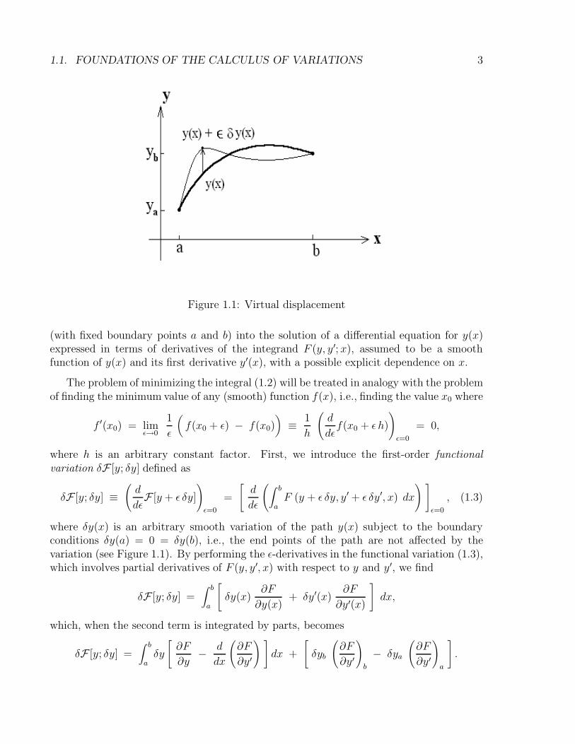
1.1. FOUNDATIONS OF THE CALCULUS OF VARIATIONS 3
Figure 1.1: Virtual displacement
(with fixed boundary points a and b) into the solution of a differential equation for y(x)expressed in terms of derivatives of the integrand F (y, y′; x), assumed to be a smoothfunction of y(x) and its first derivative y′(x), with a possible explicit dependence on x.
The problem of minimizing the integral (1.2) will be treated in analogy with the problemof finding the minimum value of any (smooth) function f(x), i.e., finding the value x0 where
f ′(x0) = limε→0
1
ε
(f(x0 + ε) − f(x0)
)≡ 1
h
(d
dεf(x0 + ε h)
)
ε=0
= 0,
where h is an arbitrary constant factor. First, we introduce the first-order functionalvariation δF [y; δy] defined as
δF [y; δy] ≡(d
dεF [y + ε δy]
)
ε=0
=
[d
dε
(∫ b
aF (y + ε δy, y′ + ε δy′, x) dx
) ]
ε=0
, (1.3)
where δy(x) is an arbitrary smooth variation of the path y(x) subject to the boundaryconditions δy(a) = 0 = δy(b), i.e., the end points of the path are not affected by thevariation (see Figure 1.1). By performing the ε-derivatives in the functional variation (1.3),which involves partial derivatives of F (y, y′, x) with respect to y and y′, we find
δF [y; δy] =∫ b
a
[
δy(x)∂F
∂y(x)+ δy′(x)
∂F
∂y′(x)
]
dx,
which, when the second term is integrated by parts, becomes
δF [y; δy] =∫ b
aδy
[∂F
∂y− d
dx
(∂F
∂y′
) ]
dx +
[
δyb
(∂F
∂y′
)
b
− δya
(∂F
∂y′
)
a
]
.
4 CHAPTER 1. INTRODUCTION TO THE CALCULUS OF VARIATIONS
Here, since the variation δy(x) vanishes at the integration boundaries (δyb = 0 = δya), thelast terms involving δyb and δya vanish explicitly and we obtain
δF [y; δy] =∫ b
aδy
[∂F
∂y− d
dx
(∂F
∂y′
) ]
dx ≡∫ b
aδy
δFδy
dx, (1.4)
where δF/δy is called the functional derivative of F [y] with respect to the function y. Thestationarity condition δF [y; δy] = 0 for all variations δy yields Euler’s First equation
d
dx
(∂F
∂y′
)
≡ y′′∂2F
∂y′ ∂y′+ y′
∂2F
∂y ∂y′+
∂2F
∂x ∂y′=
∂F
∂y, (1.5)
representing a second-order ordinary differential equation for y(x). According to the Cal-culus of Variations, the solution y(x) to this ordinary differential equation, subject to theboundary conditions y(a) = ya and y(b) = yb, yields a solution to the problem of minimiz-ing the integral (1.2). Lastly, we note that Lagrange’s variation operator δ, while analogousto the derivative operator d, commutes with the integral operator, i.e.,
δ∫ b
aP (y(x)) dx =
∫ b
aP ′(y(x)) δy(x) dx,
for any smooth function P .
Extremal Values of an Integral
Euler’s First Equation (1.5) results from the stationarity condition δF [y; δy] = 0, whichdoes not necessarily imply that the Euler path y(x), in fact, minimizes the integral (1.2).To investigate whether the path y(x) actually minimizes Eq. (1.2), we must evaluate thesecond-order functional variation
δ2F [y; δy] ≡(d2
dε2F [y + ε δy]
)
ε=0
.
By following steps similar to the derivation of Eq. (1.4), the second-order variation isexpressed as
δ2F [y; δy] =∫ b
a
δy2
[∂2F
∂y2− d
dx
(∂2F
∂y∂y′
) ]
+ (δy′)2 ∂2F
∂(y′)2
dx. (1.6)
The necessary and sufficient condition for a minimum is δ2F > 0 and, thus, the sufficientconditions for a minimal integral are
∂2F
∂y2− d
dx
(∂2F
∂y∂y′
)
> 0 and∂2F
(∂y′)2> 0, (1.7)
1.1. FOUNDATIONS OF THE CALCULUS OF VARIATIONS 5
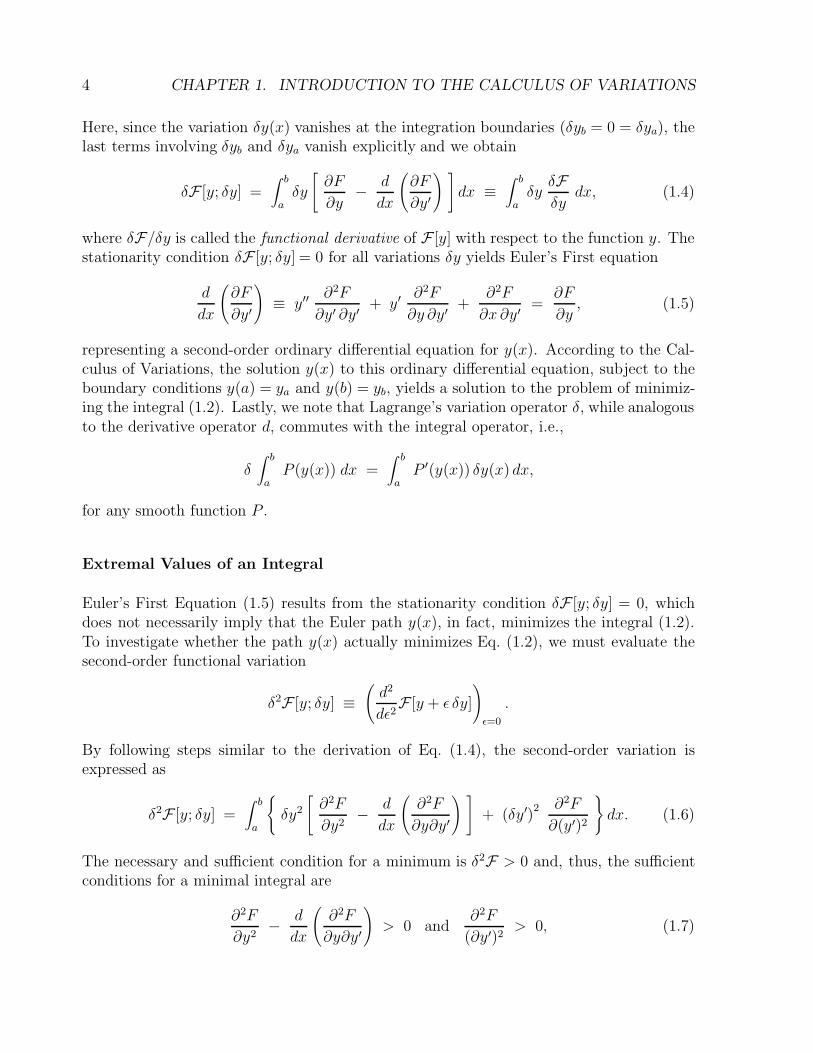
Figure 1.2: Jacobi deviation from two extremal curves
for all smooth variations δy(x). For a small enough interval (a, b), the (δy′)2-term willnormally dominate over the (δy)2-term and the sufficient condition becomes ∂2F/(∂y′)2 >0.
Because variational problems often involve finding the minima or maxima of certainintegrals, the methods of the Calculus of Variations enable us to find extermal solutionsy0(x) for which the integral F [y] is stationary (i.e., δF [y0] = 0), without specifying whetherthe second-order variation is positive-definite (corresponding to a minimum), negative-definite (corresponding to a maximum), or with indefinite sign (i.e., when the coefficientsof (δy)2 and (δy′)2 have opposite signs).
Jacobi Equation*
Carl Gustav Jacobi (1804-1851) derived a useful differential equation describing the devi-ation u(x) = y(x) − y(x) between two extremal curves (see Figure 1.2) that solve Euler’sFirst Equation (1.5) for a given function F (x, y, y′). Upon Taylor expanding Euler’s FirstEquation (1.5) for y = y + u and keeping only linear terms in u (which is assumed to besmall), we easily obtain the linear ordinary differential equation
d
dx
(
u′∂2F
(∂y′)2+ u
∂2F
∂y∂y′
)
= u∂2F
∂y2+ u′
∂2F
∂y′∂y. (1.8)
By performing the x-derivative on the second term on the left side, we obtain a partialcancellation with the second term on the right side and find the Jacobi equation
d
dx
(∂2F
(∂y′)2
du
dx
)
= u
[∂2F
∂y2− d
dx
(∂2F
∂y∂y′
) ]
. (1.9)
We can, thus, immediately see that the extremal properties (1.7) of the solutions of Euler’sFirst Equation (1.5) are intimately connected to the behavior of the deviation u(x) betweentwo nearby extremal curves.
6 CHAPTER 1. INTRODUCTION TO THE CALCULUS OF VARIATIONS
For example, if we simply assume that the coefficients in Jacobi’s equation (1.9) areboth positive (or both negative) constants ±α2 and ±β2, respectively (i.e., the extremalcurves are either minimal or maximal), then Jacobi’s equation becomes α2 u′′ = β2 u,with exponential solutions u(x) = a eγ x + b e−γ x, where (a, b) are determined from initialconditions and γ = β/α. On the other hand, if we assume that the coefficients are constants±α2 and ∓β2 of opposite signs (i.e., the extremals are neither minimal nor maximal), thenJacobi’s equation becomes α2 u′′ = −β2 u, with periodic solutions u(x) = a cos(γ x) +b sin(γ x), where (a, b) are determined from initial conditions and γ = β/α. The specialcase where the coefficient on the right side of Jacobi’s equation (1.9) vanishes (i.e., F isindependent of y) yields a differential equation for u(x) whose solution is independent ofthe sign of the coefficient ∂2F/∂(y′)2 (i.e., identical solutions are obtained for minimal andmaximal curves).
We note that the differential equation (1.8) may be derived from the variational principleδ∫J(u, u′) dx = 0 as the Jacobi-Euler equation
d
dx
(∂J
∂u′
)
=∂J
∂u, (1.10)
where the Jacobi function J(u, u′; x) is defined as
J(u, u′) ≡ 1
2
(d2
dε2F (y + ε u, y′ + ε u′)
)
ε=0
≡ u2
2
∂2F
∂y2+ uu′
∂2F
∂y∂y′+
u′2
2
∂2F
(∂y′)2. (1.11)
For example, for F (y, y′) =√
1 + (y′)2 =√
1 +m2 ≡ Λ, then ∂2F/∂y2 = 0 = ∂2F/∂y∂y′
and ∂2F/∂(y′)2 = Λ−3, and the Jacobi function becomes J(u, u′) = 12Λ−3(u′)2. The Jacobi
equation (1.9), therefore, becomes (Λ−3 u′)′ = 0, or u′′ = 0, i.e., deviations diverge linearly.
Lastly, the second functional variation (1.6) can be combined with the Jacobi equation(1.9) to yield the expression
δ2F [y; δy] =∫ b
a
∂2F
(∂y′)2
(
δy′ − δyu′
u
)2
dx,
where u(x) is a solution of the Jacobi equation (1.9). We note that the minimum conditionδ2F > 0 is now clearly associated with the condition ∂2F/∂(y′)2 > 0. Furthermore, wenote that the Jacobi equation describing space-time geodesic deviations plays a fundamentalrole in Einstein’s Theory of General Relativity. We shall return to the Jacobi equation inSec. 1.4 where we briefly discuss Fermat’s Principle of Least Time and its applications tothe general theory of geometric optics.

1.1. FOUNDATIONS OF THE CALCULUS OF VARIATIONS 7
Euler’s Second Equation
Under certain conditions (∂F/∂x ≡ 0), we may obtain a partial solution to Euler’s FirstEquation (1.5). This partial solution is derived as follows. First, we write the exact x-derivative of F (y, y′; x) as
dF
dx=
∂F
∂x+ y′
∂F
∂y+ y′′
∂F
∂y′,
and substitute Eq. (1.5) to combine the last two terms so that we obtain Euler’s Secondequation
d
dx
(
F − y′∂F
∂y′
)
=∂F
∂x. (1.12)
This equation is especially useful when the integrand F (y, y′) in Eq. (1.2) is independentof x, for which Eq. (1.12) yields the solution
F (y, y′) − y′∂F
∂y′(y, y′) = α, (1.13)
where the constant α is determined from the condition y(x0) = y0 and y′(x0) = y′0. Here,Eq. (1.13) is a partial solution (in some sense) of Eq. (1.5), since we have reduced thederivative order from second-order derivative y′′(x) in Eq. (1.5) to first-order derivativey′(x) in Eq. (1.13) on the solution y(x). Hence, Euler’s Second Equation has produced anequation of the form G(y, y′;α) = 0, which can often be integrated by quadrature as weshall see later.
1.1.3 Path of Shortest Distance and Geodesic Equation
We now return to the problem of minimizing the length integral (1.1), with the integrand
written as F (y, y′) =√
1 + (y′)2. Here, Euler’s First Equation (1.5) yields
d
dx
(∂F
∂y′
)
=y′′
[1 + (y′)2]3/2=
∂F
∂y= 0,
so that the function y(x) that minimizes the length integral (1.1) is the solution of thedifferential equation y′′(x) = 0 subject to the boundary conditions y(0) = 0 and y(1) = m,i.e., y(x) = mx. Note that the integrand F (y, y′) also satisfies the sufficient minimumconditions (1.7) so that the path y(x) = mx is indeed the path of shortest distance betweentwo points on the plane.
Geodesic equation*
We generalize the problem of finding the path of shortest distance on the Euclidean plane(x, y) to the problem of finding geodesic paths in arbitrary geometry because it introduces
8 CHAPTER 1. INTRODUCTION TO THE CALCULUS OF VARIATIONS
important geometric concepts in Classical Mechanics needed in later chapters. For thispurpose, let us consider a path in space from point A to point B parametrized by thecontinuous parameter σ, i.e., x(σ) such that x(A) = xA and x(B) = xB. The lengthintegral from point A to B is
L[x] =∫ B
A
(
gijdxi
dσ
dxj
dσ
)1/2
dσ, (1.14)
where the space metric gij is defined so that the squared infinitesimal length element isds2 ≡ gij(x) dxi dxj (summation over repeated indices is implied throughout the text).Next, using the definition (1.3), the first-order variation δL[x] is given as
δL[x] =1
2
∫ B
A
[∂gij∂xk
δxkdxi
dσ
dxj
dσ+ 2 gij
dδxi
dσ
dxj
dσ
]dσ
ds/dσ
=1
2
∫ b
a
[∂gij∂xk
δxkdxi
ds
dxj
ds+ 2 gij
dδxi
ds
dxj
ds
]
ds,
where a = s(A) and b = s(B) and we have performed a parametrization change: x(σ) →x(s). By integrating the second term by parts, we obtain
δL[x] = −∫ b
a
[d
ds
(
gijdxj
ds
)
− 1
2
∂gjk∂xi
dxj
ds
dxk
ds
]
δxi ds
= −∫ b
a
[
gijd2xj
ds2+
(∂gij∂xk
− 1
2
∂gjk∂xi
)dxj
ds
dxk
ds
]
δxi ds. (1.15)
We now note that, using symmetry properties under interchange of the j-k indices, thesecond term in Eq. (1.15) can also be written as
(∂gij∂xk
− 1
2
∂gjk∂xi
)dxj
ds
dxk
ds=
1
2
(∂gij∂xk
+∂gik∂xj
− ∂gjk∂xi
)dxj
ds
dxk
ds
= Γi|jkdxj
ds
dxk
ds,
using the definition of the Christoffel symbol
Γ`jk = g`i Γi|jk =g`i
2
(∂gij∂xk
+∂gik∂xj
− ∂gjk∂xi
)
≡ Γikj, (1.16)
where gij denotes a component of the inverse metric (i.e., gij gjk = δi k). Hence, the first-order variation (1.15) can be expressed as
δL[x] =∫ b
a
[d2xi
ds2+ Γijk
dxj
ds
dxk
ds
]
gi` δx` ds. (1.17)
1.1. FOUNDATIONS OF THE CALCULUS OF VARIATIONS 9
The stationarity condition δL = 0 for arbitrary variations δx` yields an equation for thepath x(s) of shortest distance known as the geodesic equation
d2xi
ds2+ Γijk
dxj
ds
dxk
ds= 0. (1.18)
Returning to two-dimensional Euclidean geometry, where the components of the metrictensor are constants (either 0 or 1), the geodesic equations are x′′(s) = 0 = y′′(s) whichonce again leads to a straight line.
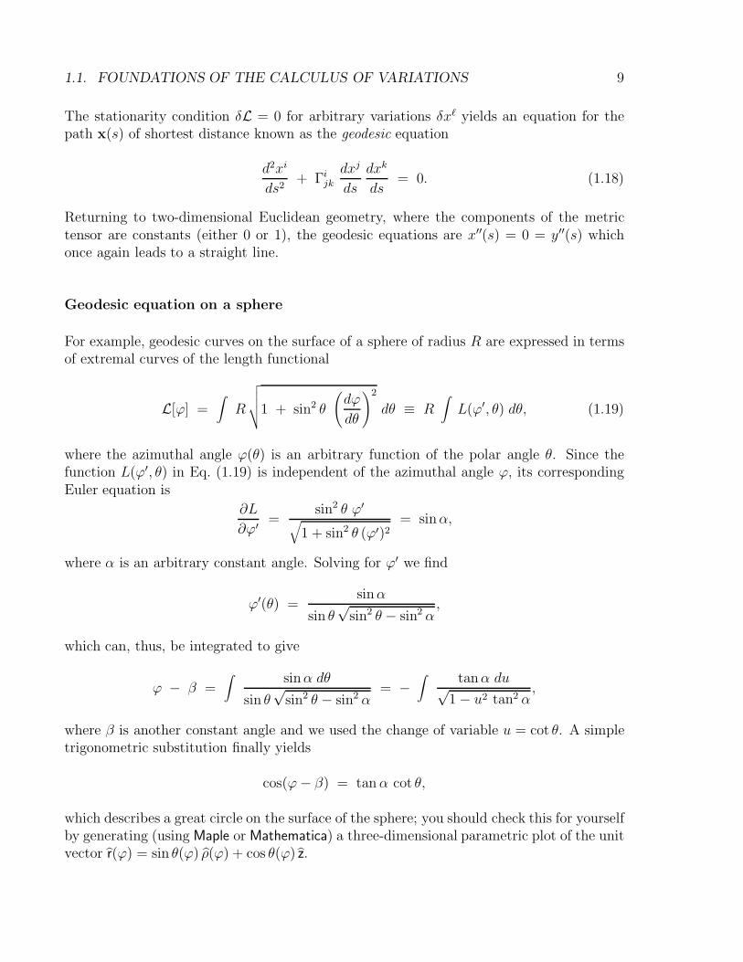
Geodesic equation on a sphere
For example, geodesic curves on the surface of a sphere of radius R are expressed in termsof extremal curves of the length functional
L[ϕ] =∫
R
√√√√1 + sin2 θ
(dϕ
dθ
)2
dθ ≡ R∫L(ϕ′, θ) dθ, (1.19)
where the azimuthal angle ϕ(θ) is an arbitrary function of the polar angle θ. Since thefunction L(ϕ′, θ) in Eq. (1.19) is independent of the azimuthal angle ϕ, its correspondingEuler equation is
∂L
∂ϕ′ =sin2 θ ϕ′
√1 + sin2 θ (ϕ′)2
= sinα,
where α is an arbitrary constant angle. Solving for ϕ′ we find
ϕ′(θ) =sinα
sin θ√
sin2 θ − sin2 α,
which can, thus, be integrated to give
ϕ − β =∫
sinα dθ
sin θ√
sin2 θ − sin2 α= −
∫tanα du√
1 − u2 tan2 α,
where β is another constant angle and we used the change of variable u = cot θ. A simpletrigonometric substitution finally yields
cos(ϕ− β) = tanα cot θ,
which describes a great circle on the surface of the sphere; you should check this for yourselfby generating (using Maple or Mathematica) a three-dimensional parametric plot of the unitvector r(ϕ) = sin θ(ϕ) ρ(ϕ) + cos θ(ϕ) z.
10 CHAPTER 1. INTRODUCTION TO THE CALCULUS OF VARIATIONS
1.2 Classical Variational Problems
The development of the Calculus of Variations led to the resolution of several classical op-timization problems in mathematics and physics. In this section, we present two classicalvariational problems that were connected to its original development. First, in the Isoperi-metric problem, we show how Lagrange modified Euler’s formulation of the Calculus ofVariations by allowing constraints to be imposed on the search for finding extremal valuesof certain integrals. Next, in the Brachistochrone problem, we show how the Calculus ofVariations is used to find the path of quickest descent for a bead sliding along a frictionlesswire under the action of gravity.
1.2.1 Isoperimetric Problem
Isoperimetric problems represent some of the earliest applications of the variational ap-proach to solving mathematical optimization problems. Pappus (ca. 290-350) was amongthe first to recognize that among all the isoperimetric closed planar curves (i.e., closedcurves that have the same perimeter length), the circle encloses the greatest area.1 Thevariational formulation of the isoperimetric problem requires that we maximize the area
integral A =∫y(x) dx while keeping the perimeter length integral L =
∫ √1 + (y′)2 dx
constant.
The isoperimetric problem falls in a class of variational problems called constrainedvariational principles, where a certain functional
∫f(y, y′, x) dx is to be optimized under
the constraint that another functional∫g(y, y′, x) dx be held constant (say at value G).
The constrained variational principle is then expressed in terms of the functional
Fλ[y] =∫f(y, y′, x) dx + λ
(G −
∫g(y, y′, x) dx
)
=∫ [
f(y, y′, x) − λ g(y, y′, x)]dx + λG, (1.20)
where the parameter λ is called a Lagrange multiplier. Note that the functional Fλ[y] ischosen, on the one hand, so that the derivative
dFλ[y]
dλ= G −
∫g(y, y′, x) dx = 0
enforces the constraint for all curves y(x). On the other hand, the stationarity conditionδFλ = 0 for the functional (1.20) with respect to arbitrary variations δy(x) (which vanishat the integration boundaries) yields Euler’s First Equation:
d
dx
(∂f
∂y′− λ
∂g
∂y′
)
=∂f
∂y− λ
∂g
∂y. (1.21)
1Such results are normally described in terms of the so-called isoperimetric inequalities 4π A ≤ L2,where A denotes the area enclosed by a closed curve of perimeter length L; here, equality is satisfied bythe circle.
1.2. CLASSICAL VARIATIONAL PROBLEMS 11
Here, we assume that this second-order differential equation is to be solved subject tothe conditions y(x0) = y0 and y′(x0) = 0; the solution y(x;λ) of Eq. (1.21) is, however,parametrized by the unknown Lagrange multiplier λ.
If the integrands f(y, y′) and g(y, y′) in Eq. (1.20) are both explicitly independent of x,then Euler’s Second Equation (1.13) for the functional (1.20) becomes
d
dx
[ (
f − y′∂f
∂y′
)
− λ
(
g − y′∂g
∂y′
) ]
= 0. (1.22)
By integrating this equation we obtain(
f − y′∂f
∂y′
)
− λ
(
g − y′∂g
∂y′
)
= 0,
where the constant of integration on the right is chosen from the conditions y(x0) = y0 andy′(x0) = 0, so that the value of the constant Lagrange multiplier is now defined as
λ(x0) =f(y0, 0)
g(y0, 0).
Hence, the solution y(x) of the constrained variational problem (1.20) is now uniquelydetermined.
We return to the isoperimetric problem now represented in terms of the constrainedfunctional
Aλ[y] =∫
y dx + λ(L −
∫ √1 + (y′)2 dx
)
=∫ [
y − λ√
1 + (y′)2
]dx + λL, (1.23)
where L denotes the value of the constant-length constraint. From Eq. (1.21), the station-arity of the functional (1.23) with respect to arbitrary variations δy(x) yields
d
dx
− λy′√
1 + (y′)2
= 1,
which can be integrated to give
− λy′√
1 + (y′)2= x − x0, (1.24)
where x0 denotes a constant of integration associated with the condition y′(x0) = 0. Since
the integrands f(y, y′) = y and g(y, y′) =√
1 + (y′)2 are both explicitly independent of x,
then Euler’s Second Equation (1.22) applies, and we obtain
d
dx
y − λ√
1 + (y′)2
= 0,
12 CHAPTER 1. INTRODUCTION TO THE CALCULUS OF VARIATIONS
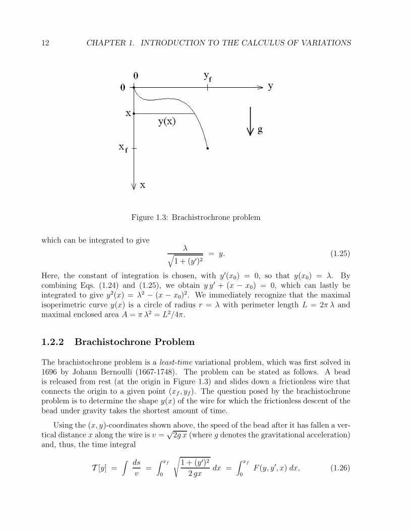
Figure 1.3: Brachistrochrone problem
which can be integrated to giveλ
√1 + (y′)2
= y. (1.25)
Here, the constant of integration is chosen, with y′(x0) = 0, so that y(x0) = λ. Bycombining Eqs. (1.24) and (1.25), we obtain y y′ + (x − x0) = 0, which can lastly beintegrated to give y2(x) = λ2 − (x − x0)
2. We immediately recognize that the maximalisoperimetric curve y(x) is a circle of radius r = λ with perimeter length L = 2π λ andmaximal enclosed area A = π λ2 = L2/4π.
1.2.2 Brachistochrone Problem
The brachistochrone problem is a least-time variational problem, which was first solved in1696 by Johann Bernoulli (1667-1748). The problem can be stated as follows. A beadis released from rest (at the origin in Figure 1.3) and slides down a frictionless wire thatconnects the origin to a given point (xf , yf). The question posed by the brachistochroneproblem is to determine the shape y(x) of the wire for which the frictionless descent of thebead under gravity takes the shortest amount of time.
Using the (x, y)-coordinates shown above, the speed of the bead after it has fallen a ver-tical distance x along the wire is v =
√2g x (where g denotes the gravitational acceleration)
and, thus, the time integral
T [y] =∫
ds
v=
∫ xf
0
√1 + (y′)2
2 gxdx =
∫ xf
0F (y, y′, x) dx, (1.26)
1.3. FERMAT’S PRINCIPLE OF LEAST TIME 13
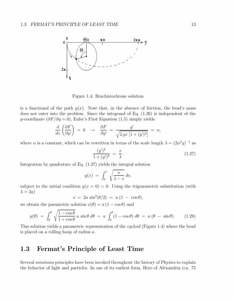
Figure 1.4: Brachistochrone solution
is a functional of the path y(x). Note that, in the absence of friction, the bead’s massdoes not enter into the problem. Since the integrand of Eq. (1.26) is independent of they-coordinate (∂F/∂y = 0), Euler’s First Equation (1.5) simply yields
d
dx
(∂F
∂y′
)
= 0 → ∂F
∂y′=
y′√
2 gx [1 + (y′)2]= α,
where α is a constant, which can be rewritten in terms of the scale length λ = (2α2g)−1 as
(y′)2
1 + (y′)2=
x
λ. (1.27)
Integration by quadrature of Eq. (1.27) yields the integral solution
y(x) =∫ x
0
√s
λ− sds,
subject to the initial condition y(x = 0) = 0. Using the trigonometric substitution (withλ = 2a)
s = 2a sin2(θ/2) = a (1 − cos θ),
we obtain the parametric solution x(θ) = a (1 − cos θ) and
y(θ) =∫ θ
0
√1 − cos θ
1 + cos θa sin θ dθ = a
∫ θ
0(1 − cos θ) dθ = a (θ − sin θ). (1.28)
This solution yields a parametric representation of the cycloid (Figure 1.4) where the beadis placed on a rolling hoop of radius a.
1.3 Fermat’s Principle of Least Time
Several minimum principles have been invoked throughout the history of Physics to explainthe behavior of light and particles. In one of its earliest form, Hero of Alexandria (ca. 75
14 CHAPTER 1. INTRODUCTION TO THE CALCULUS OF VARIATIONS
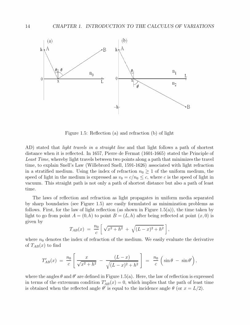
Figure 1.5: Reflection (a) and refraction (b) of light
AD) stated that light travels in a straight line and that light follows a path of shortestdistance when it is reflected. In 1657, Pierre de Fermat (1601-1665) stated the Principle ofLeast Time, whereby light travels between two points along a path that minimizes the traveltime, to explain Snell’s Law (Willebrord Snell, 1591-1626) associated with light refractionin a stratified medium. Using the index of refraction n0 ≥ 1 of the uniform medium, thespeed of light in the medium is expressed as v0 = c/n0 ≤ c, where c is the speed of light invacuum. This straight path is not only a path of shortest distance but also a path of leasttime.
The laws of reflection and refraction as light propagates in uniform media separatedby sharp boundaries (see Figure 1.5) are easily formulated as minimization problems asfollows. First, for the law of light reflection (as shown in Figure 1.5(a)), the time taken bylight to go from point A = (0, h) to point B = (L, h) after being reflected at point (x, 0) isgiven by
TAB(x) =n0
c
[ √x2 + h2 +
√(L− x)2 + h2
],
where n0 denotes the index of refraction of the medium. We easily evaluate the derivativeof TAB(x) to find
T ′AB(x) =
n0
c
x√x2 + h2
− (L − x)√
(L − x)2 + h2
=n0
c
(sin θ − sin θ′
),
where the angles θ and θ′ are defined in Figure 1.5(a). Here, the law of reflection is expressedin terms of the extremum condition T ′
AB(x) = 0, which implies that the path of least timeis obtained when the reflected angle θ′ is equal to the incidence angle θ (or x = L/2).
1.3. FERMAT’S PRINCIPLE OF LEAST TIME 15
Next, the law of light refraction (as shown in Figure 1.5(b)) involving light travellingfrom point A = (0, h) in one medium (with index of refraction n1) to point B = (L,−h)in another medium (with index of refraction n2) is similarly expressed as a minimizationproblem based on the time function
TAB(x) =1
c
[n1
√x2 + h2 + n2
√(L− x)2 + h2
],
where definitions are found in Figure 1.5(b). Here, the extremum condition T ′AB(x) = 0
yields Snell’s lawn1 sin θ = n2 sin θ′. (1.29)
Note that Snell’s law implies that the refracted light ray bends toward the medium withthe largest index of refraction. In what follows, we generalize Snell’s law to describe lightrefraction in a continuous nonuniform medium.
1.3.1 Light Propagation in a Nonuniform Medium
According to Fermat’s Principle, light propagates in a nonuniform medium by travellingalong a path that minimizes the travel time between an initial point A (where a light rayis launched) and a final point B (where the light ray is received). Hence, the time takenby a light ray following a path γ from point A to point B (parametrized by σ) is
T [x] =∫
c−1n(x)
∣∣∣∣∣dx
dσ
∣∣∣∣∣ dσ = c−1 Ln[x], (1.30)
where Ln[x] represents the length of the optical path taken by light as it travels in a mediumwith refractive index n and
∣∣∣∣∣dx
dσ
∣∣∣∣∣ =
√√√√(dx
dσ
)2
+
(dy
dσ
)2
+
(dz
dσ
)2
.
We now consider ray propagation in two dimensions (x, y), with the index of refractionn(y), and return to general properties of ray propagation in Sec. 1.4.
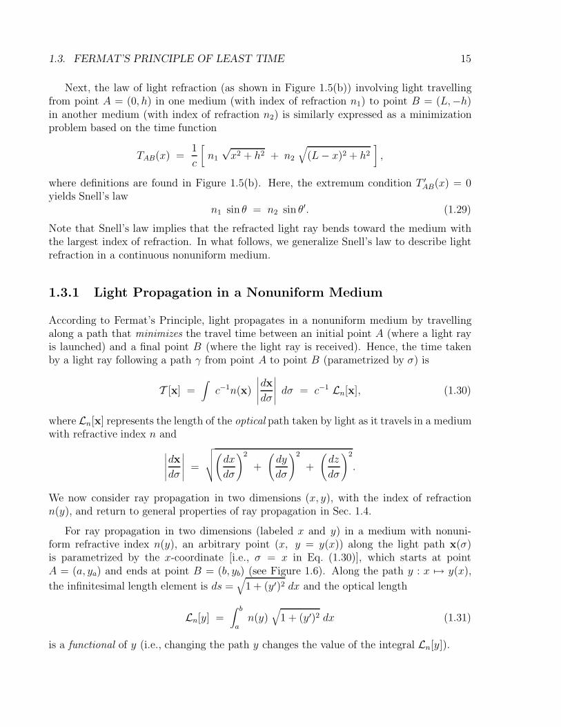
For ray propagation in two dimensions (labeled x and y) in a medium with nonuni-form refractive index n(y), an arbitrary point (x, y = y(x)) along the light path x(σ)is parametrized by the x-coordinate [i.e., σ = x in Eq. (1.30)], which starts at pointA = (a, ya) and ends at point B = (b, yb) (see Figure 1.6). Along the path y : x 7→ y(x),
the infinitesimal length element is ds =√
1 + (y′)2 dx and the optical length
Ln[y] =∫ b
an(y)
√1 + (y′)2 dx (1.31)
is a functional of y (i.e., changing the path y changes the value of the integral Ln[y]).
16 CHAPTER 1. INTRODUCTION TO THE CALCULUS OF VARIATIONS
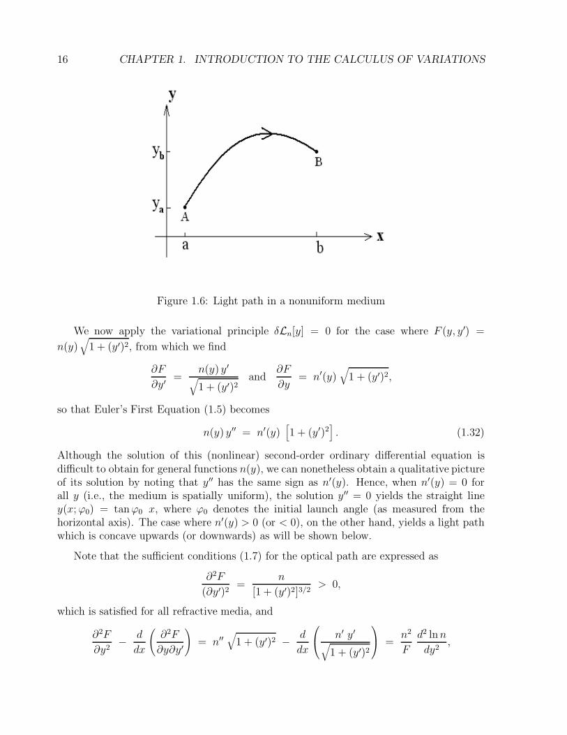
Figure 1.6: Light path in a nonuniform medium
We now apply the variational principle δLn[y] = 0 for the case where F (y, y′) =
n(y)√
1 + (y′)2, from which we find
∂F
∂y′=
n(y) y′√
1 + (y′)2and
∂F
∂y= n′(y)
√1 + (y′)2,
so that Euler’s First Equation (1.5) becomes
n(y) y′′ = n′(y)[1 + (y′)2
]. (1.32)
Although the solution of this (nonlinear) second-order ordinary differential equation isdifficult to obtain for general functions n(y), we can nonetheless obtain a qualitative pictureof its solution by noting that y′′ has the same sign as n′(y). Hence, when n′(y) = 0 forall y (i.e., the medium is spatially uniform), the solution y′′ = 0 yields the straight liney(x;ϕ0) = tanϕ0 x, where ϕ0 denotes the initial launch angle (as measured from thehorizontal axis). The case where n′(y) > 0 (or < 0), on the other hand, yields a light pathwhich is concave upwards (or downwards) as will be shown below.
Note that the sufficient conditions (1.7) for the optical path are expressed as
∂2F
(∂y′)2=
n
[1 + (y′)2]3/2> 0,
which is satisfied for all refractive media, and
∂2F
∂y2− d
dx
(∂2F
∂y∂y′
)
= n′′√
1 + (y′)2 − d
dx
n′ y′√
1 + (y′)2
=n2
F
d2 lnn
dy2,
1.3. FERMAT’S PRINCIPLE OF LEAST TIME 17
whose sign is indefinite. Hence, the sufficient condition for a minimal optical length forlight traveling in a nonuniform refractive medium is d2 lnn/dy2 > 0; note, however, thatonly the stationarity of the optical path is physically meaningful and, thus, we shall notdiscuss the minimal properties of light paths in what follows.
Since the function F (y, y′) = n(y)√
1 + (y′)2 is explicitly independent of x, we find
F − y′∂F
∂y′=
n(y)√
1 + (y′)2= constant,
and, thus, the partial solution of Eq. (1.32) is
n(y) = α√
1 + (y′)2, (1.33)
where α is a constant determined from the initial conditions of the light ray. We note thatEq. (1.33) states that as a light ray enters a region of increased (decreased) refractive index,the slope of its path also increases (decreases). In particular, by substituting Eq. (1.32)into Eq. (1.33), we find
α2 y′′ =1
2
dn2(y)
dy,
and, hence, the path of a light ray is concave upward (downward) where n′(y) is positive(negative), as previously discussed. Eq. (1.33) can be integrated by quadrature to give theintegral solution
x(y) =∫ y
0
α ds√
[n(s)]2 − α2, (1.34)
subject to the condition x(y = 0) = 0. From the explicit dependence of the index ofrefraction n(y), one may be able to perform the integration in Eq. (1.34) to obtain x(y)and, thus, obtain an explicit solution y(x) by inverting x(y).
1.3.2 Snell’s Law
We now show that the partial solution (1.33) corresponds to Snell’s Law for light refractionin a nonuniform medium. Consider a light ray travelling in the (x, y)-plane launchedfrom the initial position (0, 0) at an initial angle ϕ0 (measured from the x-axis) so thaty′(0) = tanϕ0 is the slope at x = 0. The constant α is then simply determined fromEq. (1.33) as α = n0 cosϕ0, where n0 = n(0) is the refractive index at y(0) = 0. Next, let
y′(x) = tanϕ(x) be the slope of the light ray at (x, y(x)), so that√
1 + (y′)2 = secϕ and
Eq. (1.33) becomes n(y) cosϕ = n0 cosϕ0. Lastly, when we substitute the complementaryangle θ = π/2 − ϕ (measured from the vertical y-axis), we obtain the local form of Snell’sLaw:
n[y(x)] sin θ(x) = n0 sin θ0, (1.35)
18 CHAPTER 1. INTRODUCTION TO THE CALCULUS OF VARIATIONS
properly generalized to include a light path in a nonuniform refractive medium. Note thatSnell’s Law (1.35) does not tell us anything about the actual light path y(x); this solutionmust come from solving Eq. (1.34).
1.3.3 Application of Fermat’s Principle
As an application of Fermat’s Principle, we consider the propagation of a light ray in amedium with linear refractive index n(y) = n0 (1 − β y) exhibiting a constant gradientn′(y) = −n0 β. Substituting this profile into the optical-path solution (1.34), we find
x(y) =∫ y
0
cosϕ0 ds√(1 − β s)2 − cos2 ϕ0
. (1.36)
Next, we use the trigonometric substitution
y(ϕ) =1
β
(
1 − cosϕ0
cosϕ
)
, (1.37)
with ϕ = ϕ0 at (x, y) = (0, 0), so that Eq. (1.36) becomes
x(ϕ) = − cosϕ0
βln
(secϕ+ tanϕ
secϕ0 + tanϕ0
)
. (1.38)
The parametric solution (1.37)-(1.38) for the optical path in a linear medium shows thatthe path reaches a maximum height y = y(0) at a distance x = x(0) when the tangentangle ϕ is zero:
x =cosϕ0
βln(secϕ0 + tanϕ0) and y =
1 − cosϕ0
β.
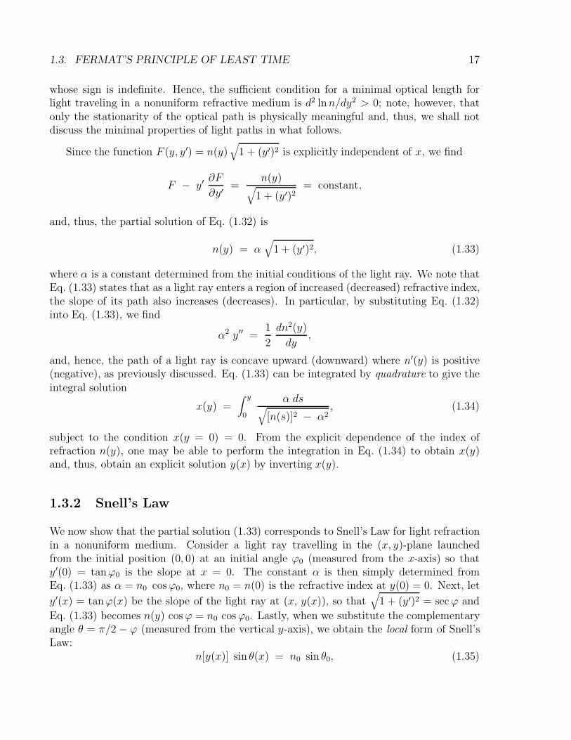
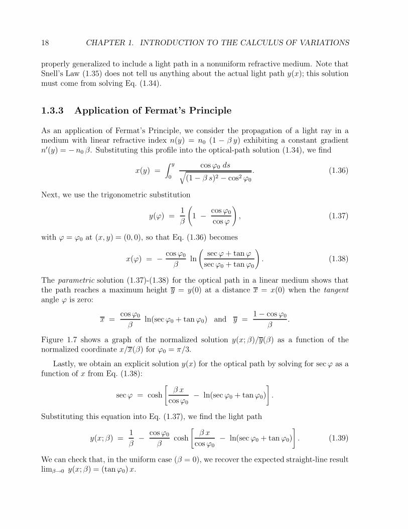
Figure 1.7 shows a graph of the normalized solution y(x; β)/y(β) as a function of thenormalized coordinate x/x(β) for ϕ0 = π/3.
Lastly, we obtain an explicit solution y(x) for the optical path by solving for secϕ as afunction of x from Eq. (1.38):
secϕ = cosh
[β x
cosϕ0− ln(secϕ0 + tanϕ0)
]
.
Substituting this equation into Eq. (1.37), we find the light path
y(x; β) =1
β− cosϕ0
βcosh
[β x
cosϕ0− ln(secϕ0 + tanϕ0)
]
. (1.39)
We can check that, in the uniform case (β = 0), we recover the expected straight-line resultlimβ→0 y(x; β) = (tanϕ0)x.
1.4. GEOMETRIC FORMULATION OF RAY OPTICS∗ 19
Figure 1.7: Light-path solution for a linear nonuniform medium
1.4 Geometric Formulation of Ray Optics∗
1.4.1 Frenet-Serret Curvature of Light Path
We now return to the general formulation for light-ray propagation based on the timeintegral (1.30), where the integrand is
F
(
x,dx
dσ
)
= n(x)
∣∣∣∣∣dx
dσ
∣∣∣∣∣ ,
and light rays are allowed to travel in a three-dimensional refractive medium with a generalindex of refraction n(x). Euler’s First equation in this case is
d
dσ
(∂F
∂(dx/dσ)
)
=∂F
∂x, (1.40)
where∂F
∂(dx/dσ)=
n
Λ
dx
dσand
∂F
∂x= Λ ∇n,
with Λ = |dx/dσ|. Euler’s First Equation (1.40), therefore, becomes
d
dσ
(n
Λ
dx
dσ
)
= Λ ∇n. (1.41)
Euler’s Second Equation, on the other hand, states that
H(σ) ≡ F
(
x,dx
dσ
)
− dx
dσ·
∂F
∂(dx/dσ)= 0
20 CHAPTER 1. INTRODUCTION TO THE CALCULUS OF VARIATIONS
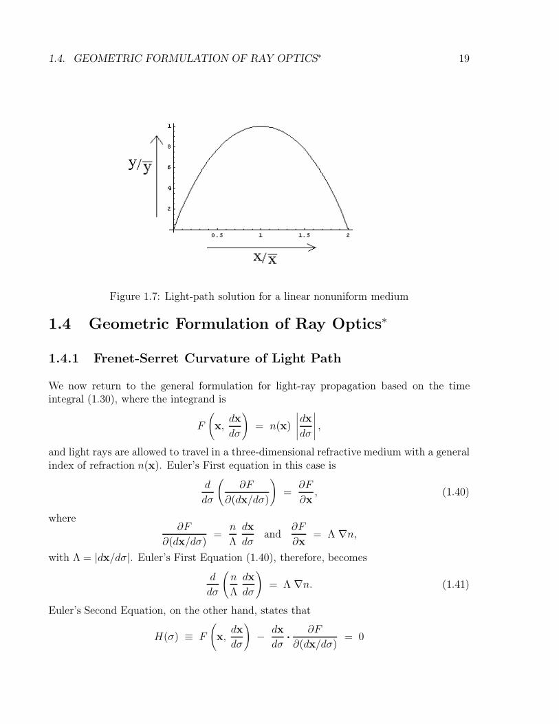
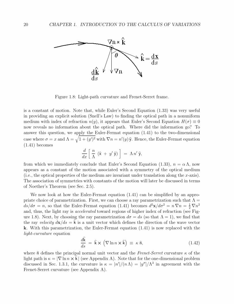
Figure 1.8: Light-path curvature and Frenet-Serret frame.
is a constant of motion. Note that, while Euler’s Second Equation (1.33) was very usefulin providing an explicit solution (Snell’s Law) to finding the optical path in a nonuniformmedium with index of refraction n(y), it appears that Euler’s Second Equation H(σ) ≡ 0now reveals no information about the optical path. Where did the information go? Toanswer this question, we apply the Euler-Fermat equation (1.41) to the two-dimensional
case where σ = x and Λ =√
1 + (y′)2 with ∇n = n′(y) y. Hence, the Euler-Fermat equation
(1.41) becomesd
dx
[n
Λ(x + y′ y)
]= Λn′ y,
from which we immediately conclude that Euler’s Second Equation (1.33), n = αΛ, nowappears as a constant of the motion associated with a symmetry of the optical medium(i.e., the optical properties of the medium are invariant under translation along the x-axis).The association of symmetries with constants of the motion will later be discussed in termsof Noether’s Theorem (see Sec. 2.5).
We now look at how the Euler-Fermat equation (1.41) can be simplified by an appro-priate choice of parametrization. First, we can choose a ray parametrization such that Λ =ds/dσ = n, so that the Euler-Fermat equation (1.41) becomes d2x/dσ2 = n∇n = 1
2∇n2
and, thus, the light ray is accelerated toward regions of higher index of refraction (see Fig-ure 1.8). Next, by choosing the ray parametrization dσ = ds (so that Λ = 1), we find thatthe ray velocity dx/ds = k is a unit vector which defines the direction of the wave vectork. With this parametrization, the Euler-Fermat equation (1.41) is now replaced with thelight-curvature equation
dk
ds= k ×
(∇ lnn× k
)≡ κ n, (1.42)
where n defines the principal normal unit vector and the Frenet-Serret curvature κ of thelight path is κ = |∇ lnn× k | (see Appendix A). Note that for the one-dimensional problemdiscussed in Sec. 1.3.1, the curvature is κ = |n′|/(nΛ) = |y′′|/Λ3 in agreement with theFrenet-Serret curvature (see Appendix A).
1.4. GEOMETRIC FORMULATION OF RAY OPTICS∗ 21
Lastly, we introduce the general form of Snell’s Law (1.35) as follows. First, we define theunit vector g = ∇n/(|∇n|) to be pointing in the direction of increasing index of refractionand, after performing the cross-product of Eq. (1.41) with g, we obtain the identity
g ×d
ds
(
ndx
ds
)
= g ×∇n = 0.
Using this identity, we readily evaluate the s-derivative of n g × k:
d
ds
(
g ×ndx
ds
)
=dg
ds×
(
ndx
ds
)
=dg
ds×n k.
Hence, if the unit vector g is constant along the path of a light ray (i.e., dg/ds = 0), wethen find the conservation law
d
ds
(g ×n k
)= 0, (1.43)
which implies that the vector quantity n g × k is a constant along the light path. Notethat, when a light ray progagates in two dimensions, this conservation law implies that thequantity |g ×n k| = n sin θ is also a constant along the light path, where θ is the angledefined as cos θ ≡ g · k. The conservation law (1.43), therefore, represents a generalizationof Snell’s Law (1.35).
1.4.2 Light Propagation in Spherical Geometry
By using the general ray-orbit equation (1.42), we can also show that for a spherically-symmetric nonuniform medium with index of refraction n(r), the light-ray orbit r(s) sat-isfies the conservation law
d
ds
(
r×n(r)dr
ds
)
= r×d
ds
(
n(r)dr
ds
)
= r×∇n(r) = 0. (1.44)
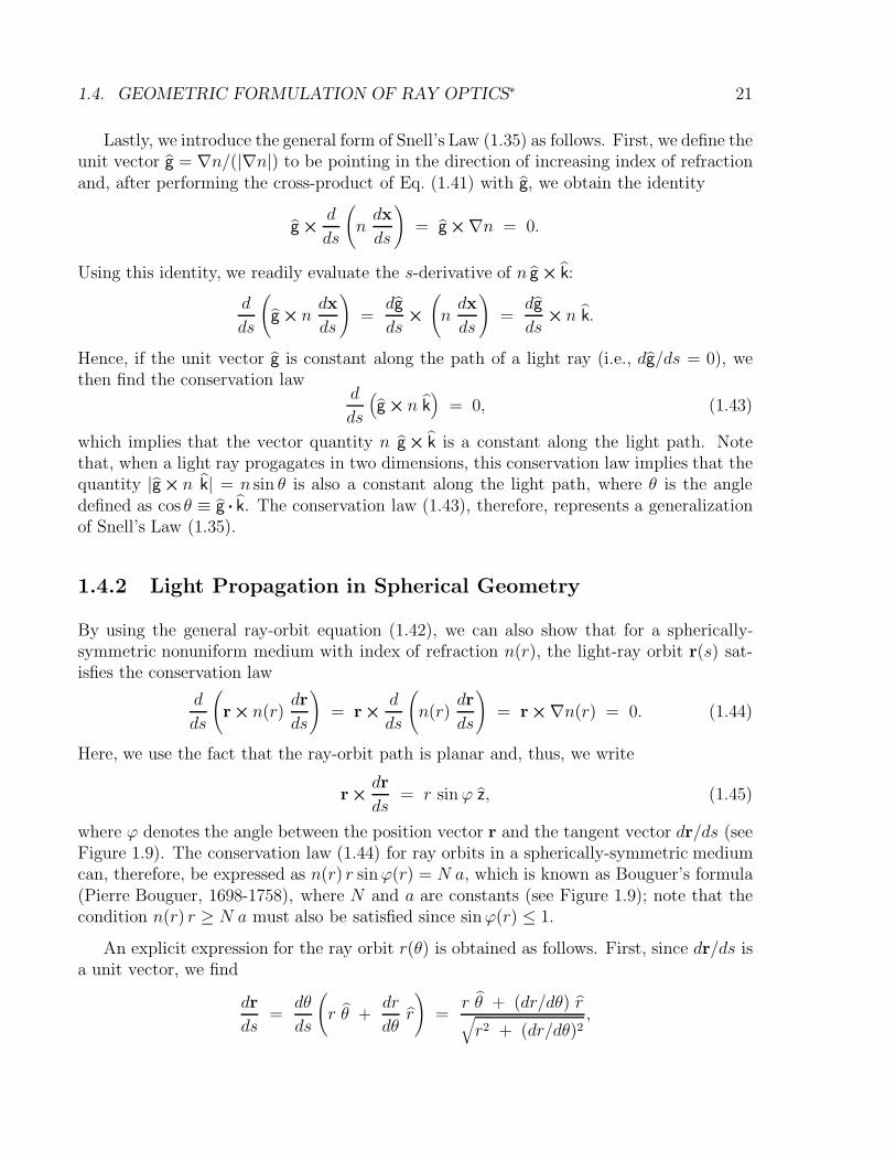
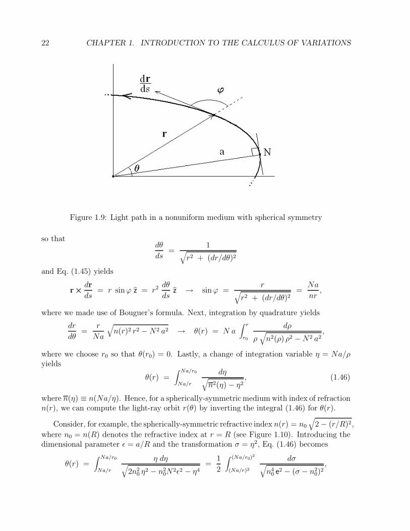
Here, we use the fact that the ray-orbit path is planar and, thus, we write
r×dr
ds= r sinϕ z, (1.45)
where ϕ denotes the angle between the position vector r and the tangent vector dr/ds (seeFigure 1.9). The conservation law (1.44) for ray orbits in a spherically-symmetric mediumcan, therefore, be expressed as n(r) r sinϕ(r) = N a, which is known as Bouguer’s formula(Pierre Bouguer, 1698-1758), where N and a are constants (see Figure 1.9); note that thecondition n(r) r ≥ N a must also be satisfied since sinϕ(r) ≤ 1.
An explicit expression for the ray orbit r(θ) is obtained as follows. First, since dr/ds isa unit vector, we find
dr
ds=
dθ
ds
(
r θ +dr
dθr
)
=r θ + (dr/dθ) r√r2 + (dr/dθ)2
,
22 CHAPTER 1. INTRODUCTION TO THE CALCULUS OF VARIATIONS
Figure 1.9: Light path in a nonuniform medium with spherical symmetry
so thatdθ
ds=
1√r2 + (dr/dθ)2
and Eq. (1.45) yields
r×dr
ds= r sinϕ z = r2 dθ
dsz → sinϕ =
r√r2 + (dr/dθ)2
=Na
nr,
where we made use of Bouguer’s formula. Next, integration by quadrature yields
dr
dθ=
r
Na
√n(r)2 r2 −N2 a2 → θ(r) = N a
∫ r
r0
dρ
ρ√n2(ρ) ρ2 −N2 a2
,
where we choose r0 so that θ(r0) = 0. Lastly, a change of integration variable η = Na/ρyields
θ(r) =∫ Na/r0
Na/r
dη√n2(η) − η2
, (1.46)
where n(η) ≡ n(Na/η). Hence, for a spherically-symmetric medium with index of refractionn(r), we can compute the light-ray orbit r(θ) by inverting the integral (1.46) for θ(r).
Consider, for example, the spherically-symmetric refractive index n(r) = n0
√2 − (r/R)2,
where n0 = n(R) denotes the refractive index at r = R (see Figure 1.10). Introducing thedimensional parameter ε = a/R and the transformation σ = η2, Eq. (1.46) becomes
θ(r) =∫ Na/r0
Na/r
η dη√
2n20 η
2 − n20N
2ε2 − η4=
1
2
∫ (Na/r0)2
(Na/r)2
dσ√n4
0 e2 − (σ − n20)
2,

1.4. GEOMETRIC FORMULATION OF RAY OPTICS∗ 23
Figure 1.10: Elliptical light path in a spherically-symmetric refractive medium.
where e =√
1 −N2ε2/n20 (assuming that n0 > N ε). Next, using the trigonometric substi-
tution σ = n20 (1 + e cosχ), we find θ(r) = 1
2χ(r) or
r2(θ) =r20 (1 + e)
1 + e cos 2θ,
which represents an ellipse of major radius and minor radius r1 = R (1 + e)1/2 and r0 =R (1− e)1/2, respectively. This example shows that, surprisingly, it is possible to trap light!
1.4.3 Geodesic Representation of Light Propagation
We now investigate the geodesic properties of light propagation in a nonuniform refractivemedium. For this purpose, let us consider a path AB in space from point A to point Bparametrized by the continuous parameter σ, i.e., x(σ) such that x(A) = xA and x(B) =xB. The time taken by light in propagating from A to B is
T [x] =∫ B
A
dt
dσdσ =
∫ B
A
n
c
(
gijdxi
dσ
dxj
dσ
)1/2
dσ, (1.47)
where dt = nds/c denotes the infinitesimal time interval taken by light in moving aninfinitesimal distance ds in a medium with refractive index n and the space metric isdenoted by gij . The geodesic properties of light propagation are investigated with thevacuum metric gij or the medium-modified metric gij = n2 gij .
24 CHAPTER 1. INTRODUCTION TO THE CALCULUS OF VARIATIONS
Vacuum-metric case
We begin with the vacuum-metric case and consider the light-curvature equation (1.42).First, we define the vacuum-metric tensor gij = ei · ej in terms of the basis vectors (e1, e2, e3),so that the ray velocity is
dx
ds=
dxi
dsei.
Second, using the definition for the Christoffel symbol (1.16) and the relations
dejds
≡ Γijkdxk
dsei,
we finddk
ds≡ d2x
ds2=
d2xi
ds2ei +
dxi
ds
deids
=
(d2xi
ds2+ Γijk
dxj
ds
dxk
ds
)
ei.
By combining these relations, light-curvature equation (1.42) becomes
d2xi
ds2+ Γijk
dxj
ds
dxk
ds=
(
gij − dxi
ds
dxj
ds
)∂ lnn
∂xj. (1.48)
This equation shows that the path of a light ray departs from a vacuum geodesic line as aresult of a refractive-index gradient projected along the tensor
hij ≡ gij − dxi
ds
dxj
ds
which, by construction, is perpendicular to the ray velocity dx/ds (i.e., hij dxj/ds = 0).
Medium-metric case
Next, we investigate the geodesic propagation of a light ray associated with the medium-modified (conformal) metric gij = n2 gij , where c2dt2 = n2ds2 = gij dx
idxj. The derivationfollows a variational formulation similar to that found in Sec. 1.1.3. Hence, the first-ordervariation δT [x] is expressed as
δT [x] =∫ tB
tA
[d2xi
dt2+ Γ
ijk
dxj
dt
dxk
dt
]
gi` δx` dt
c2, (1.49)
where the medium-modified Christoffel symbols Γijk include the effects of the gradient in
the refractive index n(x). We, therefore, find that the light path x(t) is a solution of thegeodesic equation
d2xi
dt2+ Γ
ijk
dxj
dt
dxk
dt= 0, (1.50)
which is also the path of least time for which δT [x] = 0.
1.4. GEOMETRIC FORMULATION OF RAY OPTICS∗ 25
Jacobi equation for light propagation
Lastly, we point out that the Jacobi equation for the deviation ξ(σ) = x(σ) − x(σ) be-tween two rays that satisfy the Euler-Fermat ray equation (1.41) can be obtained from theJacobian function
J(ξ, dξ/dσ) ≡ 1
2
[d2
dε2
(
n(x + ε ξ)
∣∣∣∣∣dx
dσ+ ε
dξ
dσ
∣∣∣∣∣
) ]
ε=0
≡ n
2Λ3
∣∣∣∣∣dξ
dσ×dx
dσ
∣∣∣∣∣
2
+ξ ·∇n
Λ
dξ
dσ·dx
dσ+
Λ
2ξξ : ∇∇n, (1.51)
where the Euler-Fermat ray equation (1.41) was taken into account and the exact σ-derivative, which cancels out upon integration, is omitted. Hence, the Jacobi equationdescribing light-ray deviation is expressed as the Jacobi-Euler-Fermat equation
d
dσ
(∂J
∂(dξ/dσ)
)
=∂J
∂ξ,
which yields
d
dσ
[n
Λ3
dx
dσ×
(dξ
dσ×dx
dσ
) ]
= Λ ξ ·∇∇n ·
(
I − 1
Λ2
dx
dσ
dx
dσ
)
+
[dξ
dσ− (ξ ·∇ lnn)
dx
dσ
]
×
(∇nΛ
×dx
dσ
)
. (1.52)
The Jacobi equation (1.52) describes the property of nearby rays to converge or diverge ina nonuniform refractive medium. Note, here, that the terms involving Λ−1∇n× dx/dσ inEq. (1.52) can be written in terms of the Euler-Fermat ray equation (1.41) as
∇nΛ
×dx
dσ=
1
Λ2
d
dσ
(n
Λ
dx
dσ
)
×dx
dσ=
n
Λ3
(d2x
dσ2×dx
dσ
)
,
which, thus, involve the Frenet-Serret ray curvature.
1.4.4 Eikonal Representation
The complementary picture of rays propagating in a nonuniform medium was proposed byChristiaan Huygens (1629-1695) in terms of wavefronts. Here, a wavefront is defined as thesurface that is locally perpendicular to a ray. Hence, the index of refraction itself (for anisotropic medium) can be written as
n = |∇S| =ck
ωor ∇S = n
dx
ds=
ck
ω, (1.53)
26 CHAPTER 1. INTRODUCTION TO THE CALCULUS OF VARIATIONS
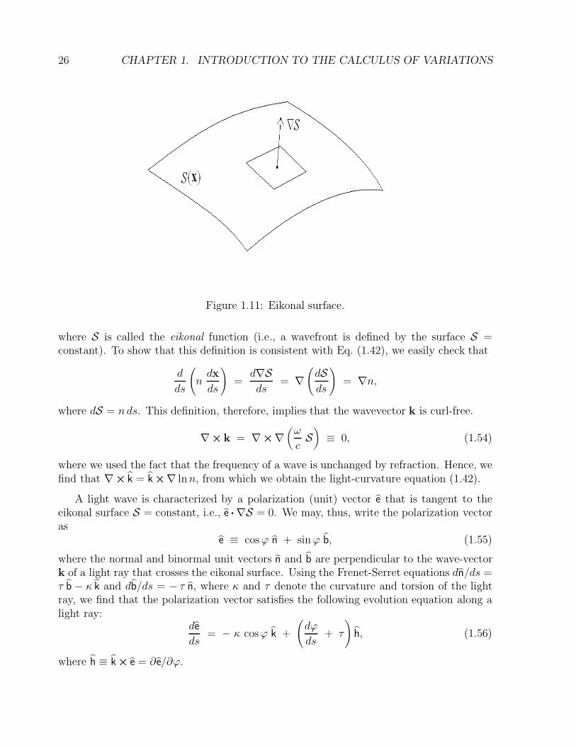
Figure 1.11: Eikonal surface.
where S is called the eikonal function (i.e., a wavefront is defined by the surface S =constant). To show that this definition is consistent with Eq. (1.42), we easily check that
d
ds
(
ndx
ds
)
=d∇Sds
= ∇(dSds
)
= ∇n,
where dS = nds. This definition, therefore, implies that the wavevector k is curl-free.
∇×k = ∇×∇(ω
cS)
≡ 0, (1.54)
where we used the fact that the frequency of a wave is unchanged by refraction. Hence, wefind that ∇× k = k ×∇ lnn, from which we obtain the light-curvature equation (1.42).
A light wave is characterized by a polarization (unit) vector e that is tangent to theeikonal surface S = constant, i.e., e ·∇S = 0. We may, thus, write the polarization vectoras
e ≡ cosϕ n + sinϕ b, (1.55)
where the normal and binormal unit vectors n and b are perpendicular to the wave-vectork of a light ray that crosses the eikonal surface. Using the Frenet-Serret equations dn/ds =τ b − κ k and db/ds = − τ n, where κ and τ denote the curvature and torsion of the lightray, we find that the polarization vector satisfies the following evolution equation along alight ray:
de
ds= − κ cosϕ k +
(dϕ
ds+ τ
)
h, (1.56)
where h ≡ k × e = ∂e/∂ϕ.
1.4. GEOMETRIC FORMULATION OF RAY OPTICS∗ 27
Note that, in the absence of sources and sinks, the light energy flux entering a finitevolume bounded by a closed surface is equal to the light energy flux leaving the volumeand, thus, the intensity of light I satisfies the conservation law
0 = ∇ · (I ∇S) = I ∇2S + ∇S ·∇I. (1.57)
Using the definition ∇S ·∇ ≡ n∂/∂s, we find the intensity evolution equation
∂ ln I
∂s= − n−1 ∇2S,
whose solution is expressed as
I = I0 exp
(
−∫ s
0∇2S dσ
n
)
, (1.58)
where I0 is the light intensity at position s = 0 along a ray. This equation, therefore,determines whether light intensity increases (∇2S < 0) or decreases (∇2S > 0) along a raydepending on the sign of ∇2S. Lastly, in a refractive medium with spherical symmetry,with S ′(r) = n(r) and k = r, the conservation law (1.57) becomes
0 =1
r2
d
dr
(r2 I n
),
which implies that the light intensity satisfies the inverse-square law: I(r)n(r) r2 = I0n0 r20.
28 CHAPTER 1. INTRODUCTION TO THE CALCULUS OF VARIATIONS
1.5 Problems
Problem 1
Find Euler’s first and second equations following the extremization of the integral
F [y] =∫ b
aF (y, y′, y′′) dx.
State whether an additional set of boundary conditions for δy′(a) and δy′(b) are necessary.
Problem 2
Find the curve joining two points (x1, y1) and (x2, y2) that yields a surface of revolution(about the x-axis) of minimum area by minimizing the integral
A[y] =∫ x2
x1
y√
1 + (y′)2 dx.
Problem 3
Show that the time required for a particle to move without friction to the minimum
point of the cycloid solution of the Brachistochrone problem is π√a/g.
Problem 4
A thin rope of massm (and uniform density) is attached to two vertical poles of heightHseparated by a horizontal distanceD; the coordinates of the pole tops are set at (±D/2, H).If the length L of the rope is greater than D, it will sag under the action of gravity andits lowest point (at its midpoint) will be at a height y(x = 0) = y0. The shape of therope, subject to the boundary conditions y(±D/2) = H, is obtained by minimizing thegravitational potential energy of the rope expressed in terms of the functional
U [y] =∫ −D/2
D/2mg y
√1 + (y′)2 dx.
Show that the extremal curve y(x) (known as the catenary curve) for this problem is
y(x) = c cosh
(x− b
c
)
,
where b = 0 and c = y0.
1.5. PROBLEMS 29
Problem 5
A light ray travels in a medium with refractive index
n(y) = n0 exp (−β y),
where n0 is the refractive index at y = 0 and β is a positive constant.
(a) Use the results of the Principle of Least Time contained in the Notes distributed inclass to show that the path of the light ray is expressed as
y(x; β) =1
βln
[cos(β x− ϕ0)
cosϕ0
]
, (1.59)
where the light ray is initially travelling upwards from (x, y) = (0, 0) at an angle ϕ0.
(b) Using the appropriate mathematical techniques, show that we recover the expectedresult limβ→0 y(x; β) = (tanϕ0) x from Eq. (1.59).
(c) The light ray reaches a maximum height y at x = x(β), where y′(x; β) = 0. Findexpressions for x and y(β) = y(x; β).
Problem 6
Consider the path associated with the index of refraction n(y) = H/y, where the heightH is a constant and 0 < y < H α−1 ≡ R to ensure that, according to Eq. (1.33), n(y) > α.Show that the light path has the simple semi-circular form:
(R− x)2 + y2 = R2 → y(x) =√x (2R − x).
Problem 7
Using the parametric solutions (1.37)-(1.38) of the optical path in a linear refractivemedium, calculate the Frenet-Serret curvature coefficient
κ(ϕ) =|r′′(ϕ)× r′(ϕ)|
|r′(ϕ)|3 ,
and show that it is equal to |k ×∇ lnn|.
Problem 8
Assuming that the refractive index n(z) in a nonuniform medium is a function of z only,derive the Euler-Fermat equations (1.42) for the components (α, β, γ) of the unit vectork = α x + β y + γ z.
30 CHAPTER 1. INTRODUCTION TO THE CALCULUS OF VARIATIONS
Problem 9
In Figure 1.10, show that the angle ϕ(θ) defined from the conservation law (1.44) isexpressed as
ϕ(θ) = arcsin
[1 + e cos 2θ√
1 + e2 + 2 e cos 2θ
]
,
so that ϕ = π2
at θ = 0 and π2, as expected for an ellipse.
Problem 10
Find the light-path trajectory r(θ) for a spherically-symmetric medium with index ofrefraction n(r) = n0 (b/r)2, where b is an arbitrary constant and n0 = n(b).
Problem 11
Derive the Jacobi equation (1.52) for two-dimensional light propagation in a nonuniformmedium with index of refraction n(y). (Hint: choose σ = x) Compare your Jacobi equationwith that obtained from Eq. (1.9).
Chapter 2
Lagrangian Mechanics
In this Chapter, we present four principles by which single-particle dynamics may be de-scribed. Here, each principle provides an algorithm by which dynamical equations arederived.
2.1 Maupertuis-Jacobi’s Principle of Least Action
The publication of Fermat’s Principle of Least Time in 1657 generated an intense contro-versy between Fermat and disciples of Rene Descartes (1596-1650) involving whether lighttravels slower (Fermat) or faster (Descartes) in a dense medium as compared to free space.
In 1740, Pierre Louis Moreau de Maupertuis (1698-1759) stated (without proof) that,in analogy with Fermat’s Principle of Least Time for light, a particle of mass m under theinfluence of a force F = −∇U moves along a path which satisfies the Principle of LeastAction: δS = 0, where the action integral is defined as
S[x] =∫
p · dx =∫mv ds, (2.1)
where v = ds/dt denotes the magnitude of particle velocity, which can also be expressed as
v(s) =√
(2/m) [E − U(s)], (2.2)
with the particle’s kinetic energy K = mv2/2 written in terms of its total energy E and itspotential energy U(s).
2.1.1 Maupertuis’ principle
In 1744, Euler proved Maupertuis’ Principle of Least Action δ∫mv ds = 0 for particle
motion in the (x, y)-plane as follows. For this purpose, we use the Frenet-Serret curvature
31
32 CHAPTER 2. LAGRANGIAN MECHANICS
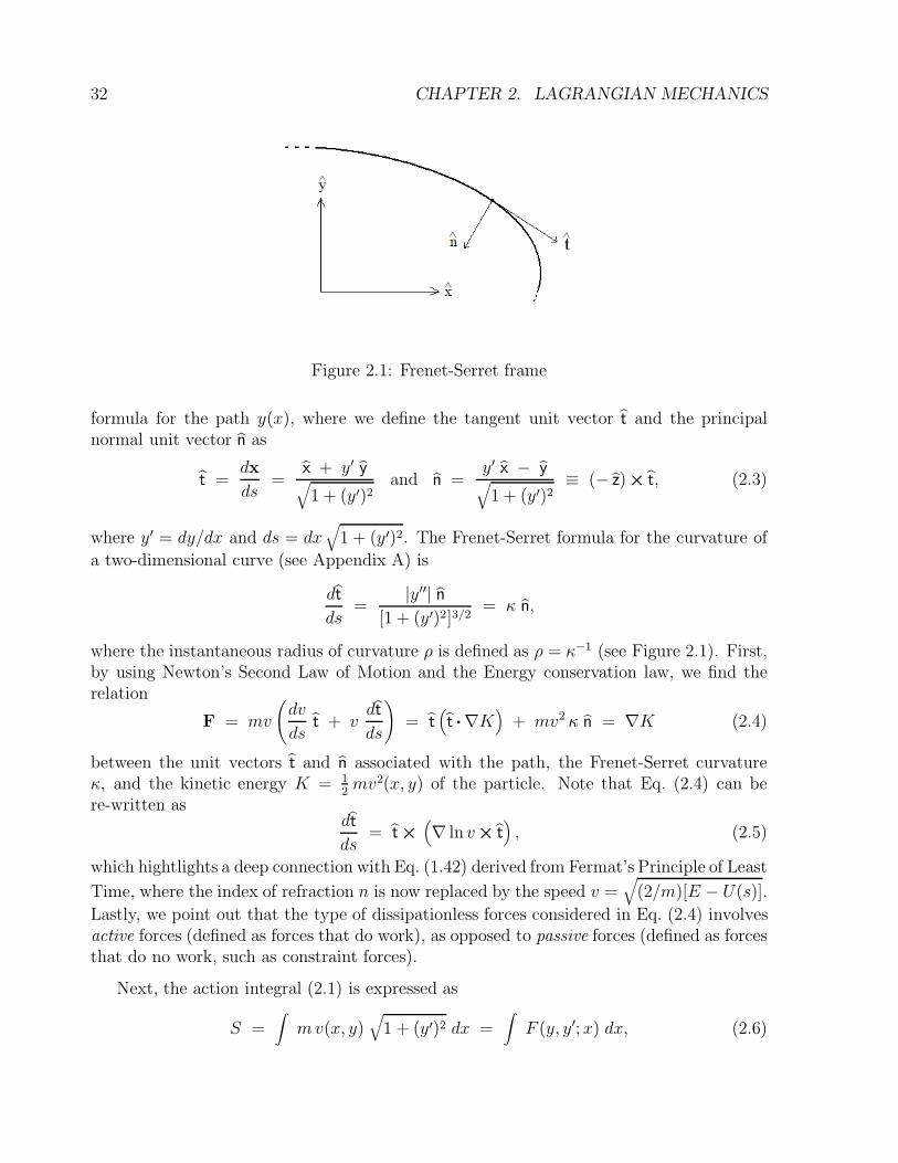
Figure 2.1: Frenet-Serret frame
formula for the path y(x), where we define the tangent unit vector t and the principalnormal unit vector n as
t =dx
ds=
x + y′ y√
1 + (y′)2and n =
y′ x − y√
1 + (y′)2≡ (− z)× t, (2.3)
where y′ = dy/dx and ds = dx√
1 + (y′)2. The Frenet-Serret formula for the curvature of
a two-dimensional curve (see Appendix A) is
dt
ds=
|y′′| n
[1 + (y′)2]3/2= κ n,
where the instantaneous radius of curvature ρ is defined as ρ = κ−1 (see Figure 2.1). First,by using Newton’s Second Law of Motion and the Energy conservation law, we find therelation
F = mv
(dv
dst + v
dt
ds
)
= t(t ·∇K
)+ mv2 κ n = ∇K (2.4)
between the unit vectors t and n associated with the path, the Frenet-Serret curvatureκ, and the kinetic energy K = 1
2mv2(x, y) of the particle. Note that Eq. (2.4) can be
re-written asdt
ds= t ×
(∇ ln v× t
), (2.5)
which hightlights a deep connection with Eq. (1.42) derived from Fermat’s Principle of Least
Time, where the index of refraction n is now replaced by the speed v =√
(2/m)[E − U(s)].
Lastly, we point out that the type of dissipationless forces considered in Eq. (2.4) involvesactive forces (defined as forces that do work), as opposed to passive forces (defined as forcesthat do no work, such as constraint forces).
Next, the action integral (2.1) is expressed as
S =∫mv(x, y)
√1 + (y′)2 dx =
∫F (y, y′; x) dx, (2.6)

2.1. MAUPERTUIS-JACOBI’S PRINCIPLE OF LEAST ACTION 33
so that the Euler’s First Equation (1.5) corresponding to Maupertuis’ action integral (2.6),with
∂F
∂y′=
mv y′√
1 + (y′)2and
∂F
∂y= m
√1 + (y′)2
∂v
∂y,
yields the Maupertuis-Euler equation
m v y′′
[1 + (y′)2]3/2=
m√
1 + (y′)2
∂v
∂y− m y′
√1 + (y′)2
∂v
∂x≡ m n ·∇v, (2.7)
which can also be expressed as mv κ = m n ·∇v. Using the relation F = ∇K and theFrenet-Serret formulas (2.3), the Maupertuis-Euler equation (2.7) becomes
mv2 κ = F · n,
from which we recover Newton’s Second Law (2.4).
2.1.2 Jacobi’s principle
Jacobi emphasized the connection between Fermat’s Principle of Least Time (1.30) andMaupertuis’ Principle of Least Action (2.1) by introducing a different form of the Principleof Least Action δS = 0, where Jacobi’s action integral is
S[x] =∫ √
2m (E − U) ds = 2∫K dt, (2.8)
where particle momentum is written as p =√
2m (E − U). To obtain the second expression
of Jacobi’s action integral (2.8), Jacobi made use of the fact that, by introducing a pathparameter τ such that v = ds/dt = s′/t′ (where a prime, here, denotes a τ -derivative), wefind
K =m (s′)2
2 (t′)2= E − U,
so that 2K t′ = s′ p, and the second form of Jacobi’s action integral results. Next, Jacobiused the Principle of Least Action (2.8) to establish the geometric foundations of particlemechanics. Here, the Euler-Jacobi equation resulting from Jacobi’s Principle of LeastAction is expressed as
d
ds
(√E − U
dx
ds
)
= ∇√E − U ,
which is identical in form to the light-curvature equation (1.42), with the index of refractionn substituted with
√E − U .
Note that the connection between Fermat’s Principle of Least Time and Maupertuis-Jacobi’s Principle of Least Action involves the relation n = γ |p|, where γ is a constant.

34 CHAPTER 2. LAGRANGIAN MECHANICS
This connection was later used by Prince Louis Victor Pierre Raymond de Broglie (1892-1987) to establish the relation |p| = h|k| = n (hω/c) between the momentum of a particleand its wavenumber |k| = 2π/λ = nω/c. Using de Broglie’s relation p = h k between theparticle momentum p and the wave vector k, we note that
|p|22m
=h2|k|22m
≡ h2
2m|∇Θ|2 = E − U, (2.9)
where Θ is the dimensionless (eikonal) phase. Letting Θ = lnψ, so that ∇Θ = ∇ lnψ,Eq. (2.9) becomes
h2
2m|∇ψ|2 = (E − U) ψ2.
Lastly, by taking its variation
h2
m∇ψ ·∇δψ − δψ (E − U) ψ = 0,
and integrating over space (upon integration by parts), we obtain
0 =∫
Vδψ
[
(E − U) ψ +h2
2m∇2ψ
]
d3x,
which yields (for arbitrary variations δψ) the time-independent Schrodinger equation
− h2
2m∇2ψ + U ψ = E ψ.
Further historical comments concerning the derivation of Schrodinger’s equation can befound in Yougrau and Mandelstam’s (Variational Principles in Dynamics and QuantumTheory, 1968).
2.2 D’Alembert’s Principle
So far, we have studied the Maupertuis-Jacobi principles (2.1) and (2.8), which make use ofthe length variable s as the orbit parameter to describe particle motion. We now turn ourattention to two principles that will provide a clear path toward the ultimate variationalprinciple called Hamilton’s Principle, from which equations of motion are derived in termsof generalized spatial coordinates.
First, within the context of Newtonian mechanics, we distinguish between two classes offorces, depending on whether a force is able to do work or not. In the first class, an activeforce Fw is involved in performing infinitesimal work dW = Fw · dx evaluated along theinfinitesimal displacement dx; the class of active forces includes conservative (e.g., gravity)and nonconservative (e.g., friction) forces. In the second class, a passive force (labeled F0)is defined as a force not involved in performing work, which includes constraint forces suchas normal and tension forces. Here, the infinitesimal work performed by a passive force isF0 · dx = 0 because the infinitesimal displacement dx is required to satisfy the constraints.
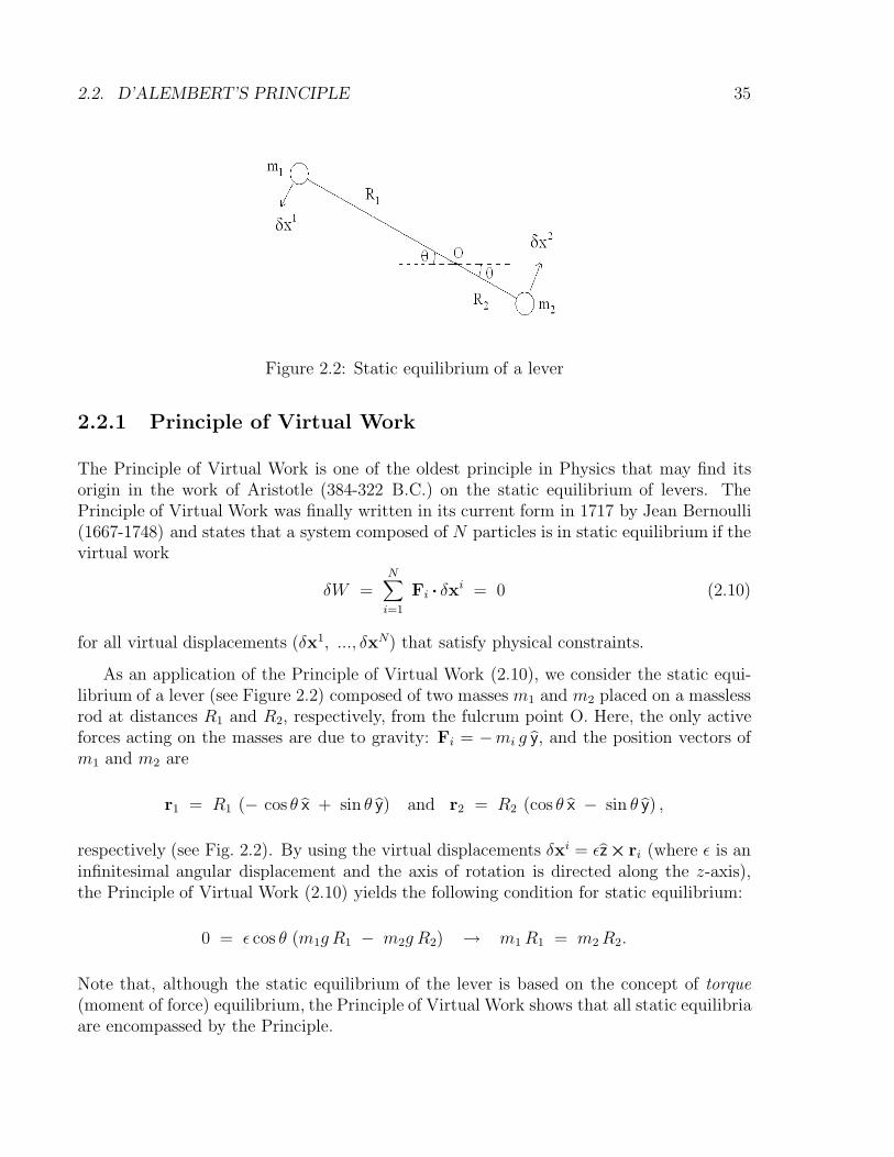
2.2. D’ALEMBERT’S PRINCIPLE 35
Figure 2.2: Static equilibrium of a lever
2.2.1 Principle of Virtual Work
The Principle of Virtual Work is one of the oldest principle in Physics that may find itsorigin in the work of Aristotle (384-322 B.C.) on the static equilibrium of levers. ThePrinciple of Virtual Work was finally written in its current form in 1717 by Jean Bernoulli(1667-1748) and states that a system composed of N particles is in static equilibrium if thevirtual work
δW =N∑
i=1
Fi · δxi = 0 (2.10)
for all virtual displacements (δx1, ..., δxN) that satisfy physical constraints.
As an application of the Principle of Virtual Work (2.10), we consider the static equi-librium of a lever (see Figure 2.2) composed of two masses m1 and m2 placed on a masslessrod at distances R1 and R2, respectively, from the fulcrum point O. Here, the only activeforces acting on the masses are due to gravity: Fi = −mi g y, and the position vectors ofm1 and m2 are
r1 = R1 (− cos θ x + sin θ y) and r2 = R2 (cos θ x − sin θ y) ,
respectively (see Fig. 2.2). By using the virtual displacements δxi = εz× ri (where ε is aninfinitesimal angular displacement and the axis of rotation is directed along the z-axis),the Principle of Virtual Work (2.10) yields the following condition for static equilibrium:
0 = ε cos θ (m1g R1 − m2g R2) → m1R1 = m2R2.
Note that, although the static equilibrium of the lever is based on the concept of torque(moment of force) equilibrium, the Principle of Virtual Work shows that all static equilibriaare encompassed by the Principle.

36 CHAPTER 2. LAGRANGIAN MECHANICS
2.2.2 Lagrange’s Equations from D’Alembert’s Principle
It was Jean Le Rond d’Alembert (1717-1783) who generalized the Principle of Virtual Work(in 1742) by including the accelerating force −mi x
i in the Principle of Virtual Work (2.10):
N∑
i=1
(
Fi − mid2xi
dt2
)
· δxi = 0 (2.11)
so that the equations of dynamics could be obtained from Eq. (2.11). Hence, d’Alembert’sPrinciple, in effect, states that the work done by all active forces acting in a system isalgebraically equal to the work done by all the acceleration forces (taken to be positive).
As a simple application of d’Alembert’s Principle (2.11), we return to the lever problem(see Fig. 2.2), where we now assume m2R2 > m1R1. Here, the particle accelerations are
xi = − (θ)2 ri − θ z × ri,
so that d’Alembert’s Principle (2.11) yields (with δxi = ε z × ri)
0 = ε[
(m1g R1 − m2g R2) cos θ +(m1R
21 + m2R
22
)θ].
Hence, according to d’Alembert’s Principle, the angular acceleration θ of the unbalancedlever is
θ =g cos θ
I(m2R2 − m1R1) ,
where I = m1R21 + m2R
22 denotes the moment of inertia of the lever as it rotates about
the fulcrum point O. Thus, we see that rotational dynamics associated with unbalancedtorques can be described in terms of d’Alembert’s Principle.
The most historically significant application of d’Alembert’s Principle (2.11), however,came from Lagrange who transformed it as follows. Consider, for simplicity, the followinginfinitesimal-work identity
0 =
(
F − md2x
dt2
)
· δx = δW − d
dt
(
mdx
dt· δx
)
+ mdx
dt·d δx
dt, (2.12)
where F denotes an active force applied to a particle of mass m so that δW = F · δx denotesthe virtual work calculated along the virtual displacement δx. We note that if the positionvector x(q1, ..., qk; t) is a time-dependent function of k generalized coordinates, then we find
δx =k∑
i=1
∂x
∂qiδqi,
and
v =dx
dt=
∂x
∂t+
k∑
i=1
∂x
∂qiqi.
2.2. D’ALEMBERT’S PRINCIPLE 37
Next, we introduce the variation of the kinetic energy K = mv2/2:
δK = mdx
dt·d δx
dt=
∑
i
δqi∂K
∂qi,
since the virtual variation operator δ (introduced by Lagrange) commutes with the timederivative d/dt, and we introduce the generalized force
Qi ≡ F ·∂x
∂qi,
so that δW =∑i Q
i δqi. We shall also use the identity
md2x
dt2·∂x
∂qi=
d
dt
(
mv ·∂x
∂qi
)
− mv ·d
dt
(∂x
∂qi
)
,
withd
dt
(∂x
∂qi
)
≡ ∂2x
∂t ∂qi+ qj
∂2x
∂qj ∂qi≡ ∂v
∂qi,
and∂v
∂qi=
∂x
∂qi.
Our first result derived from D’Alembert’s Principle (2.12) is now expressed in terms of thegeneralized coordinates (q1, ..., qk) as
0 =∑
i
δqi
[d
dt
(∂K
∂qi
)
− ∂K
∂qi− Qi
]
.
Since this relation must hold for any variation δqi (i = 1, ..., k), we obtain Lagrange’sequation
d
dt
(∂K
∂qi
)
− ∂K
∂qi= Qi, (2.13)
where we note that the generalized force Qi is associated with any active (conservative ornonconservative) force F. Hence, for a conservative active force derivable from a singlepotential energy U (i.e., F = −∇U), the ith-component of the generalized force is Qi =− ∂U/∂qi, and Lagrange’s equation (2.13) becomes
d
dt
(∂K
∂qi
)
− ∂K
∂qi= − ∂U
∂qi. (2.14)
We shall soon return to this important equation.
Our second result based on D’Alembert’s Principle (2.12), now expressed as
δK + δW =d
dt
(
mdx
dt· δx
)
, (2.15)
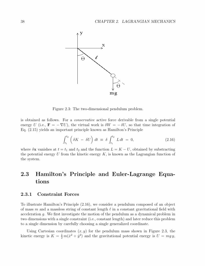
38 CHAPTER 2. LAGRANGIAN MECHANICS
Figure 2.3: The two-dimensional pendulum problem.
is obtained as follows. For a conservative active force derivable from a single potentialenergy U (i.e., F = −∇U), the virtual work is δW = − δU , so that time integration ofEq. (2.15) yields an important principle known as Hamilton’s Principle
∫ t2
t1
(δK − δU
)dt ≡ δ
∫ t2
t1Ldt = 0, (2.16)
where δx vanishes at t = t1 and t2 and the function L = K − U , obtained by substractingthe potential energy U from the kinetic energy K, is known as the Lagrangian function ofthe system.
2.3 Hamilton’s Principle and Euler-Lagrange Equa-
tions
2.3.1 Constraint Forces
To illustrate Hamilton’s Principle (2.16), we consider a pendulum composed of an objectof mass m and a massless string of constant length ` in a constant gravitational field withacceleration g. We first investigate the motion of the pendulum as a dynamical problem intwo dimensions with a single constraint (i.e., constant length) and later reduce this problemto a single dimension by carefully choosing a single generalized coordinate.
Using Cartesian coordinates (x, y) for the pendulum mass shown in Figure 2.3, thekinetic energy is K = 1
2m(x2 + y2) and the gravitational potential energy is U = mg y,
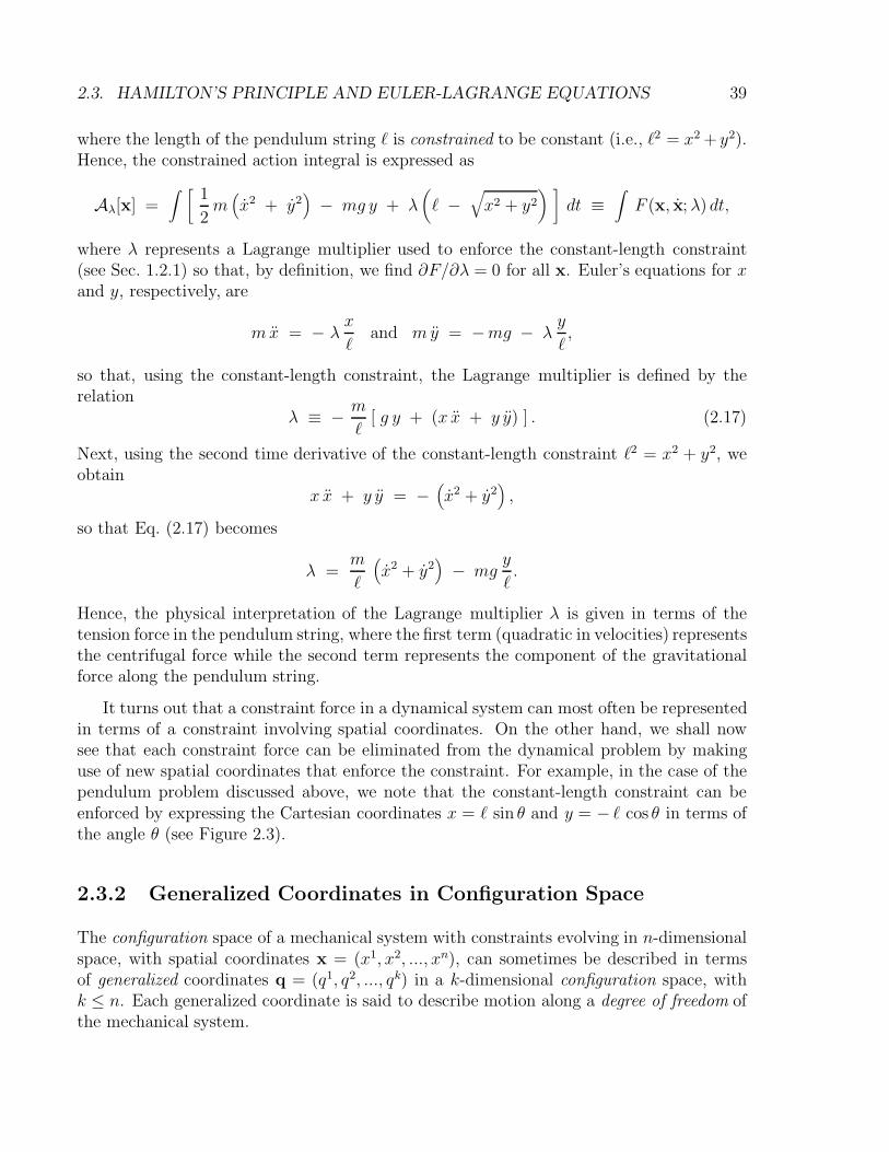
2.3. HAMILTON’S PRINCIPLE AND EULER-LAGRANGE EQUATIONS 39
where the length of the pendulum string ` is constrained to be constant (i.e., `2 = x2 + y2).Hence, the constrained action integral is expressed as
Aλ[x] =∫ [
1
2m(x2 + y2
)− mg y + λ
(` −
√x2 + y2
) ]dt ≡
∫F (x, x;λ) dt,
where λ represents a Lagrange multiplier used to enforce the constant-length constraint(see Sec. 1.2.1) so that, by definition, we find ∂F/∂λ = 0 for all x. Euler’s equations for xand y, respectively, are
mx = − λx
`and m y = −mg − λ
y
`,
so that, using the constant-length constraint, the Lagrange multiplier is defined by therelation
λ ≡ − m
`[ g y + (x x + y y) ] . (2.17)
Next, using the second time derivative of the constant-length constraint `2 = x2 + y2, weobtain
x x + y y = −(x2 + y2
),
so that Eq. (2.17) becomes
λ =m
`
(x2 + y2
)− mg
y
`.
Hence, the physical interpretation of the Lagrange multiplier λ is given in terms of thetension force in the pendulum string, where the first term (quadratic in velocities) representsthe centrifugal force while the second term represents the component of the gravitationalforce along the pendulum string.
It turns out that a constraint force in a dynamical system can most often be representedin terms of a constraint involving spatial coordinates. On the other hand, we shall nowsee that each constraint force can be eliminated from the dynamical problem by makinguse of new spatial coordinates that enforce the constraint. For example, in the case of thependulum problem discussed above, we note that the constant-length constraint can beenforced by expressing the Cartesian coordinates x = ` sin θ and y = − ` cos θ in terms ofthe angle θ (see Figure 2.3).
2.3.2 Generalized Coordinates in Configuration Space
The configuration space of a mechanical system with constraints evolving in n-dimensionalspace, with spatial coordinates x = (x1, x2, ..., xn), can sometimes be described in termsof generalized coordinates q = (q1, q2, ..., qk) in a k-dimensional configuration space, withk ≤ n. Each generalized coordinate is said to describe motion along a degree of freedom ofthe mechanical system.
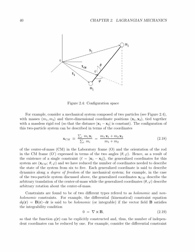
40 CHAPTER 2. LAGRANGIAN MECHANICS
Figure 2.4: Configuration space
For example, consider a mechanical system composed of two particles (see Figure 2.4),with masses (m1, m2) and three-dimensional coordinate positions (x1,x2), tied togetherwith a massless rigid rod (so that the distance |x1 − x2| is constant). The configuration ofthis two-particle system can be described in terms of the coordinates
xCM ≡∑i mi xi∑i mi
=m1 x1 +m2 x2
m1 +m2(2.18)
of the center-of-mass (CM) in the Laboratory frame (O) and the orientation of the rodin the CM frame (O’) expressed in terms of the two angles (θ, ϕ). Hence, as a result ofthe existence of a single constraint (` = |x1 − x2|), the generalized coordinates for thissystem are (xCM ; θ, ϕ) and we have reduced the number of coordinates needed to describethe state of the system from six to five. Each generalized coordinate is said to describedynamics along a degree of freedom of the mechanical system; for example, in the caseof the two-particle system discussed above, the generalized coordinates xCM describe thearbitrary translation of the center-of-mass while the generalized coordinates (θ, ϕ) describearbitrary rotation about the center-of-mass.
Constraints are found to be of two different types refered to as holonomic and non-holonomic constraints. For example, the differential (kinematical) constraint equationdq(r) = B(r) · dr is said to be holonomic (or integrable) if the vector field B satisfiesthe integrability condition
0 = ∇×B, (2.19)
so that the function q(r) can be explicitly constructed and, thus, the number of indepen-dent coordinates can be reduced by one. For example, consider the differential constraint
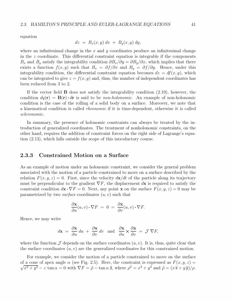
2.3. HAMILTON’S PRINCIPLE AND EULER-LAGRANGE EQUATIONS 41
equation
dz = Bx(x, y) dx + By(x, y) dy,
where an infinitesimal change in the x and y coordinates produce an infinitesimal changein the z coordinate. This differential constraint equation is integrable if the componentsBx and By satisfy the integrability condition ∂Bx/∂y = ∂By/∂x, which implies that thereexists a function f(x, y) such that Bx = ∂f/∂x and By = ∂f/∂y. Hence, under thisintegrability condition, the differential constraint equation becomes dz = df(x, y), whichcan be integrated to give z = f(x, y) and, thus, the number of independent coordinates hasbeen reduced from 3 to 2.
If the vector field B does not satisfy the integrability condition (2.19), however, thecondition dq(r) = B(r) · dr is said to be non-holonomic. An example of non-holonomiccondition is the case of the rolling of a solid body on a surface. Moreover, we note thata kinematical condition is called rheonomic if it is time-dependent, otherwise it is calledscleronomic.
In summary, the presence of holonomic constraints can always be treated by the in-troduction of generalized coordinates. The treatment of nonholonomic constraints, on theother hand, requires the addition of constraint forces on the right side of Lagrange’s equa-tion (2.13), which falls outside the scope of this introductory course.
2.3.3 Constrained Motion on a Surface
As an example of motion under an holonomic constraint, we consider the general problemassociated with the motion of a particle constrained to move on a surface described by therelation F (x, y, z) = 0. First, since the velocity dx/dt of the particle along its trajectorymust be perpendicular to the gradient ∇F , the displacement dx is required to satisfy theconstraint condition dx ·∇F = 0. Next, any point x on the surface F (x, y, z) = 0 may beparametrized by two surface coordinates (u, v) such that
∂x
∂u(u, v) ·∇F = 0 =
∂x
∂v(u, v) ·∇F.
Hence, we may write
dx =∂x
∂udu +
∂x
∂vdv and
∂x
∂u×∂x
∂v= J ∇F,
where the function J depends on the surface coordinates (u, v). It is, thus, quite clear thatthe surface coordinates (u, v) are the generalized coordinates for this constrained motion.
For example, we consider the motion of a particle constrained to move on the surfaceof a cone of apex angle α (see Fig. 2.5). Here, the constraint is expressed as F (x, y, z) =√x2 + y2 − z tanα = 0 with ∇F = ρ − tanα z, where ρ2 = x2 + y2 and ρ = (x x + y y)/ρ.
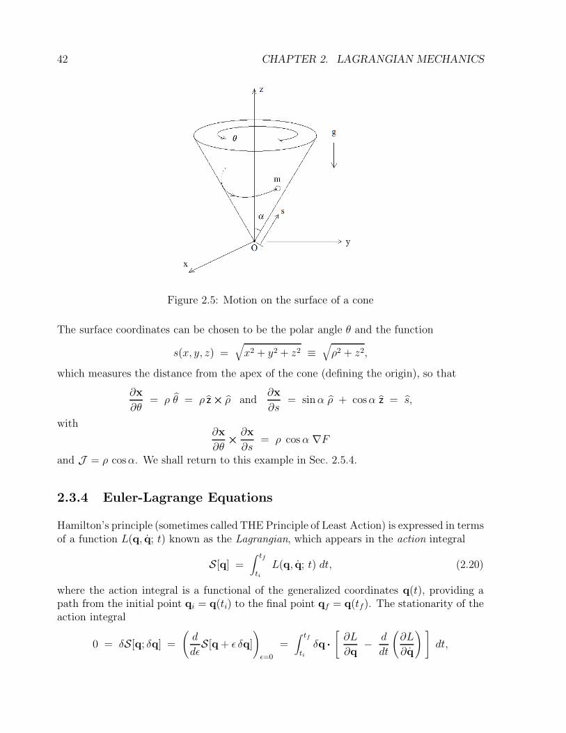
42 CHAPTER 2. LAGRANGIAN MECHANICS
Figure 2.5: Motion on the surface of a cone
The surface coordinates can be chosen to be the polar angle θ and the function
s(x, y, z) =√x2 + y2 + z2 ≡
√ρ2 + z2,
which measures the distance from the apex of the cone (defining the origin), so that
∂x
∂θ= ρ θ = ρ z × ρ and
∂x
∂s= sinα ρ + cosα z = s,
with∂x
∂θ×∂x
∂s= ρ cosα ∇F
and J = ρ cosα. We shall return to this example in Sec. 2.5.4.
2.3.4 Euler-Lagrange Equations
Hamilton’s principle (sometimes called THE Principle of Least Action) is expressed in termsof a function L(q, q; t) known as the Lagrangian, which appears in the action integral
S[q] =∫ tf
tiL(q, q; t) dt, (2.20)
where the action integral is a functional of the generalized coordinates q(t), providing apath from the initial point qi = q(ti) to the final point qf = q(tf). The stationarity of theaction integral
0 = δS[q; δq] =
(d
dεS[q + ε δq]
)
ε=0
=∫ tf
tiδq ·
[∂L
∂q− d
dt
(∂L
∂q
) ]
dt,
2.3. HAMILTON’S PRINCIPLE AND EULER-LAGRANGE EQUATIONS 43
where the variation δq is assumed to vanish at the integration boundaries (δqi = 0 = δqf),yields the Euler-Lagrange equation for the generalized coordinate qj (j = 1, ..., k):
d
dt
(∂L
∂qj
)
=∂L
∂qj. (2.21)
The Lagrangian also satisfies the second Euler equation:
d
dt
(
L − q ·∂L
∂q
)
=∂L
∂t, (2.22)
and thus, for time-independent Lagrangian systems (∂L/∂t = 0), we find that L−q · ∂L/∂qis a conserved quantity whose interpretation will be discussed shortly.
Note that, according to d’Alembert’s Principle (2.11), or Eq. (2.16), the form of theLagrangian function L(r, r; t) is dictated by our requirement that Newton’s Second Lawm r = −∇U(r, t), which describes the motion of a particle of mass m in a nonuniform(possibly time-dependent) potential U(r, t), be written in the Euler-Lagrange form (2.21).One easily obtains the form
L(r, r; t) =m
2|r|2 − U(r, t), (2.23)
for the Lagrangian of a particle of mass m, which is simply the kinetic energy of theparticle minus its potential energy. The minus sign in Eq. (2.23) is important; not onlydoes this form give us the correct equations of motion but, without the minus sign, energywould not be conserved. In fact, we note that Jacobi’s action integral (2.8) can also bewritten as A =
∫[(K − U) + E] dt, using the Energy conservation law E = K + U ; hence,
Energy conservation is the important connection between the Principles of Least Action ofMaupertuis-Jacobi and Euler-Lagrange.
For a simple mechanical system, the Lagrangian function is obtained by computing thekinetic energy of the system and its potential energy and then construct Eq. (2.23). Theconstruction of a Lagrangian function for a system of N particles, therefore, proceeds infour steps as follows.
• Step I. Define k generalized coordinates q1(t), ..., qk(t) that represent the instanta-neous configuration of the mechanical system of N particles at time t.
• Step II. For each particle, construct the position vector ra(q; t) in Cartesian coordinatesand its associated velocity
va(q, q; t) =∂ra∂t
+k∑
j=1
qj∂ra∂qj
for a = 1, ..., N .
44 CHAPTER 2. LAGRANGIAN MECHANICS
• Step III. Construct the kinetic energy
K(q, q; t) =∑
a
ma
2|va(q, q; t)|2
and the potential energyU(q; t) =
∑
a
U(ra(q; t), t)
for the system and combine them to obtain the Lagrangian
L(q, q; t) = K(q, q; t) − U(q; t).
• Step IV. From the Lagrangian L(q, q; t), the Euler-Lagrange equations (2.21) arederived for each generalized coordinate qj:
∑
a
d
dt
(∂ra∂qj
·ma va
)
=∑
a
(
ma va ·∂va∂qj
− ∂ra∂qj
·∇aU
)
, (2.24)
where we have used the identity ∂va/∂qj = ∂ra/∂q
j.
Note that in the presence of k time-dependent constraints Φj(r1, ..., rn; t) = 0 (j =1, ..., k) among n point particles, the Euler-Lagrange equation for the ith-coordinate xi` ofthe `th-particle is expressed as
d
dt
(∂L
∂xi`
)
− ∂L
∂xi`=
k∑
j=1
λj(t)∂Φj
∂xi`,
where λj(t) (j = 1, ..., k) denote the Lagrange multipliers needed to impose the constraints.
2.3.5 Lagrangian Mechanics in Curvilinear Coordinates∗
The Euler-Lagrange equation (2.24) can be framed within the context of Riemannian ge-ometry as follows; Jacobi was the first to investigate the relation between particle dynamicsand Riemannian geometry. The kinetic energy of a single particle of mass m, with gener-alized coordinates q = (q1, ..., qk), is expressed as
K =m
2|v|2 =
m
2
∂r
∂qi·∂r
∂qjqi qj ≡ m
2gij q
i qj,
where gij denotes the metric tensor on configuration space. When the particle moves in apotential U(q), the Euler-Lagrange equation (2.24) becomes
d
dt
(mgij q
j)
= mgij qj +
m
2
(∂gij∂qk
+∂gik∂qj
)
qj qk
=m
2
∂gjk∂qi
qj qk − ∂U
∂qi,
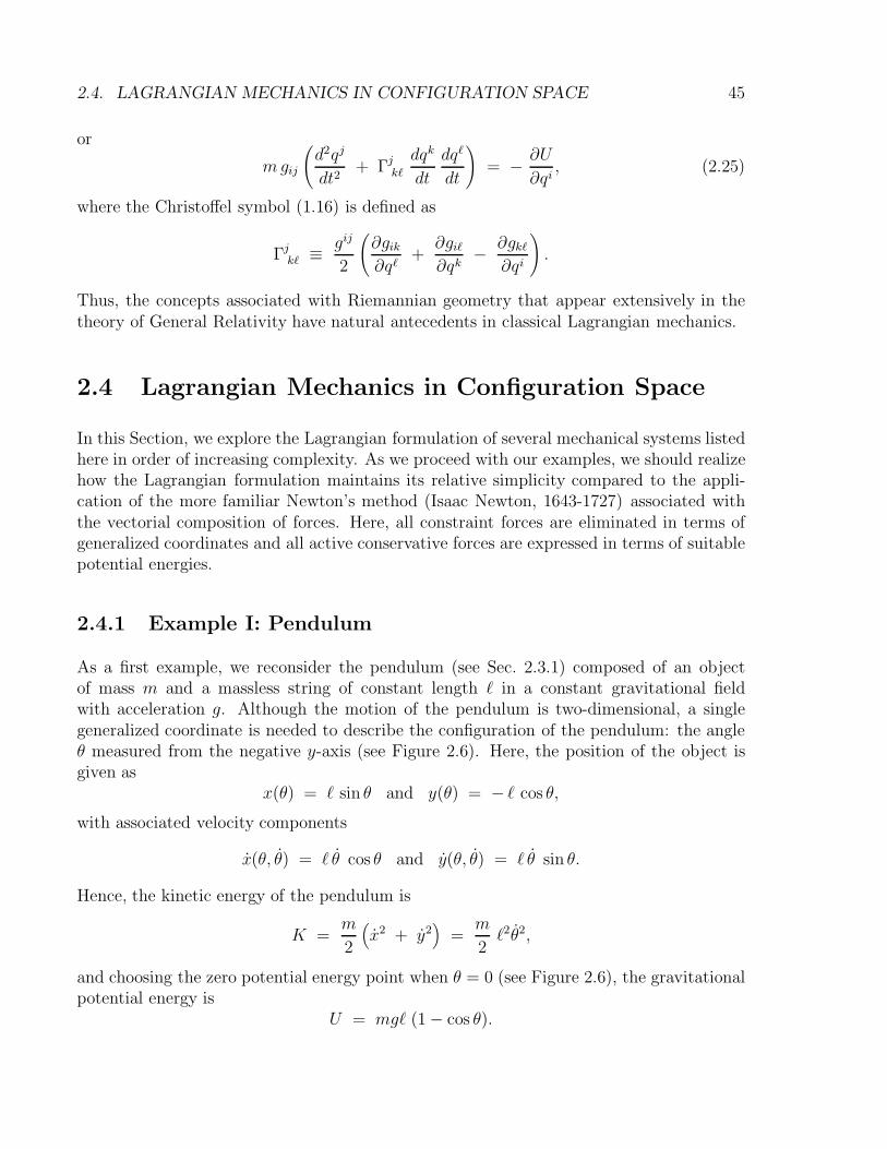
2.4. LAGRANGIAN MECHANICS IN CONFIGURATION SPACE 45
or
mgij
(d2qj
dt2+ Γjk`
dqk
dt
dq`
dt
)
= − ∂U
∂qi, (2.25)
where the Christoffel symbol (1.16) is defined as
Γjk` ≡ gij
2
(∂gik∂q`
+∂gi`∂qk
− ∂gk`∂qi
)
.
Thus, the concepts associated with Riemannian geometry that appear extensively in thetheory of General Relativity have natural antecedents in classical Lagrangian mechanics.
2.4 Lagrangian Mechanics in Configuration Space
In this Section, we explore the Lagrangian formulation of several mechanical systems listedhere in order of increasing complexity. As we proceed with our examples, we should realizehow the Lagrangian formulation maintains its relative simplicity compared to the appli-cation of the more familiar Newton’s method (Isaac Newton, 1643-1727) associated withthe vectorial composition of forces. Here, all constraint forces are eliminated in terms ofgeneralized coordinates and all active conservative forces are expressed in terms of suitablepotential energies.
2.4.1 Example I: Pendulum
As a first example, we reconsider the pendulum (see Sec. 2.3.1) composed of an objectof mass m and a massless string of constant length ` in a constant gravitational fieldwith acceleration g. Although the motion of the pendulum is two-dimensional, a singlegeneralized coordinate is needed to describe the configuration of the pendulum: the angleθ measured from the negative y-axis (see Figure 2.6). Here, the position of the object isgiven as
x(θ) = ` sin θ and y(θ) = − ` cos θ,
with associated velocity components
x(θ, θ) = ` θ cos θ and y(θ, θ) = ` θ sin θ.
Hence, the kinetic energy of the pendulum is
K =m
2
(x2 + y2
)=
m
2`2θ2,
and choosing the zero potential energy point when θ = 0 (see Figure 2.6), the gravitationalpotential energy is
U = mg` (1 − cos θ).
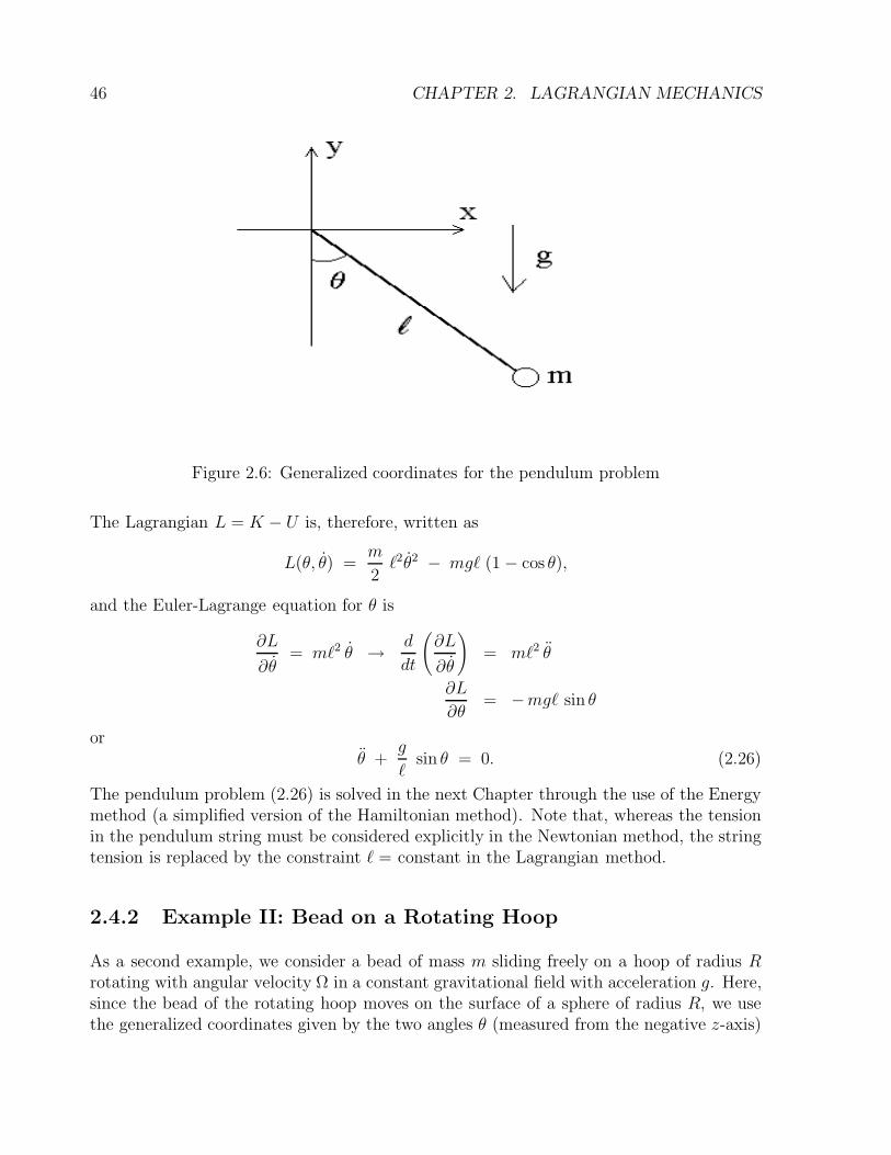
46 CHAPTER 2. LAGRANGIAN MECHANICS
Figure 2.6: Generalized coordinates for the pendulum problem
The Lagrangian L = K − U is, therefore, written as
L(θ, θ) =m
2`2θ2 − mg` (1 − cos θ),
and the Euler-Lagrange equation for θ is
∂L
∂θ= m`2 θ → d
dt
(∂L
∂θ
)
= m`2 θ
∂L
∂θ= −mg` sin θ
orθ +
g
`sin θ = 0. (2.26)
The pendulum problem (2.26) is solved in the next Chapter through the use of the Energymethod (a simplified version of the Hamiltonian method). Note that, whereas the tensionin the pendulum string must be considered explicitly in the Newtonian method, the stringtension is replaced by the constraint ` = constant in the Lagrangian method.
2.4.2 Example II: Bead on a Rotating Hoop
As a second example, we consider a bead of mass m sliding freely on a hoop of radius Rrotating with angular velocity Ω in a constant gravitational field with acceleration g. Here,since the bead of the rotating hoop moves on the surface of a sphere of radius R, we usethe generalized coordinates given by the two angles θ (measured from the negative z-axis)
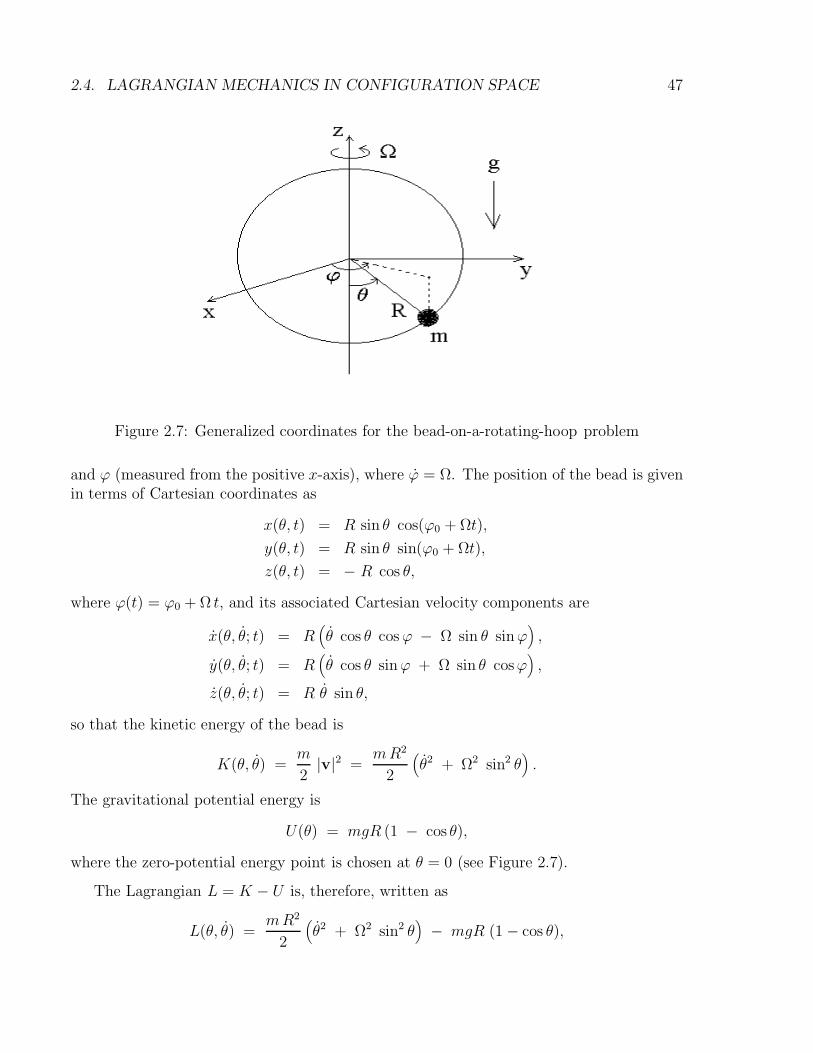
2.4. LAGRANGIAN MECHANICS IN CONFIGURATION SPACE 47
Figure 2.7: Generalized coordinates for the bead-on-a-rotating-hoop problem
and ϕ (measured from the positive x-axis), where ϕ = Ω. The position of the bead is givenin terms of Cartesian coordinates as
x(θ, t) = R sin θ cos(ϕ0 + Ωt),
y(θ, t) = R sin θ sin(ϕ0 + Ωt),
z(θ, t) = − R cos θ,
where ϕ(t) = ϕ0 + Ω t, and its associated Cartesian velocity components are
x(θ, θ; t) = R(θ cos θ cosϕ − Ω sin θ sinϕ
),
y(θ, θ; t) = R(θ cos θ sinϕ + Ω sin θ cosϕ
),
z(θ, θ; t) = R θ sin θ,
so that the kinetic energy of the bead is
K(θ, θ) =m
2|v|2 =
mR2
2
(θ2 + Ω2 sin2 θ
).
The gravitational potential energy is
U(θ) = mgR (1 − cos θ),
where the zero-potential energy point is chosen at θ = 0 (see Figure 2.7).
The Lagrangian L = K − U is, therefore, written as
L(θ, θ) =mR2
2
(θ2 + Ω2 sin2 θ
)− mgR (1 − cos θ),
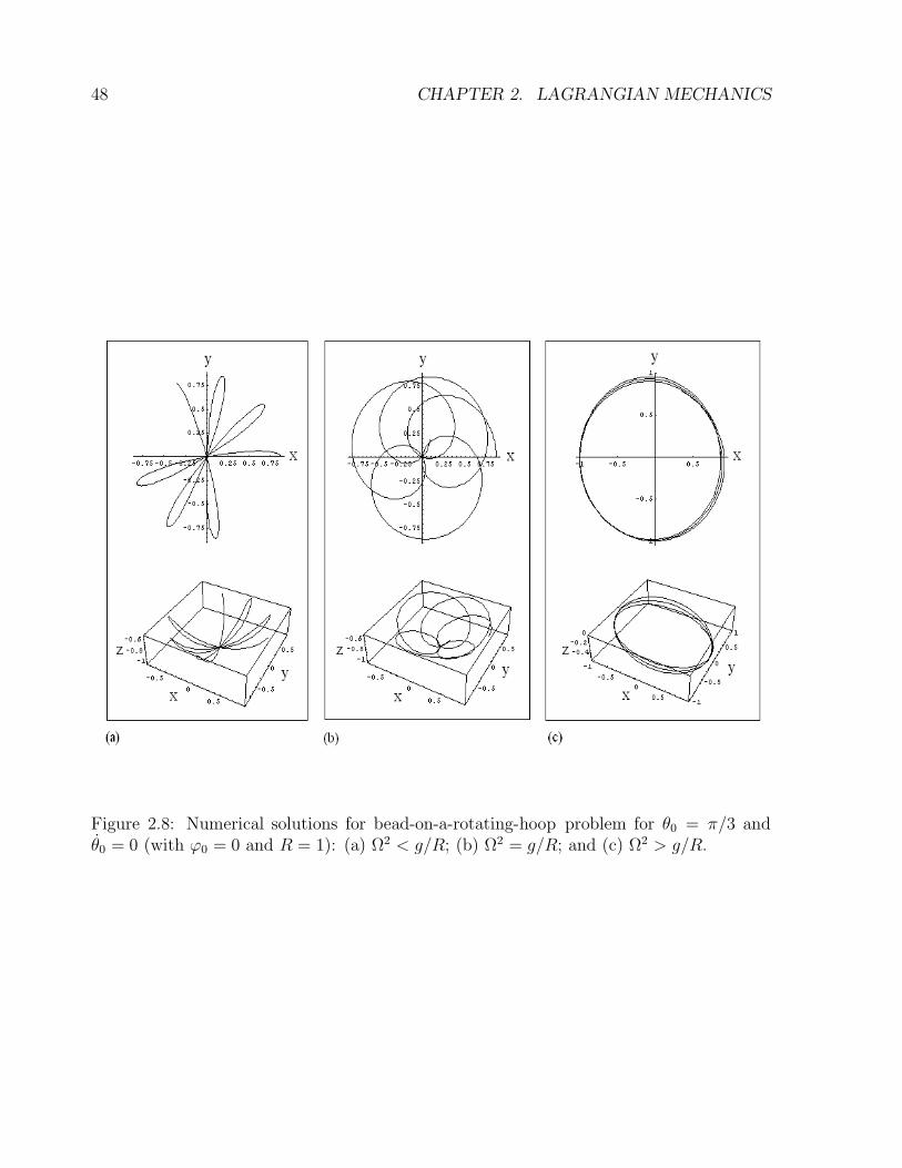
48 CHAPTER 2. LAGRANGIAN MECHANICS
Figure 2.8: Numerical solutions for bead-on-a-rotating-hoop problem for θ0 = π/3 andθ0 = 0 (with ϕ0 = 0 and R = 1): (a) Ω2 < g/R; (b) Ω2 = g/R; and (c) Ω2 > g/R.
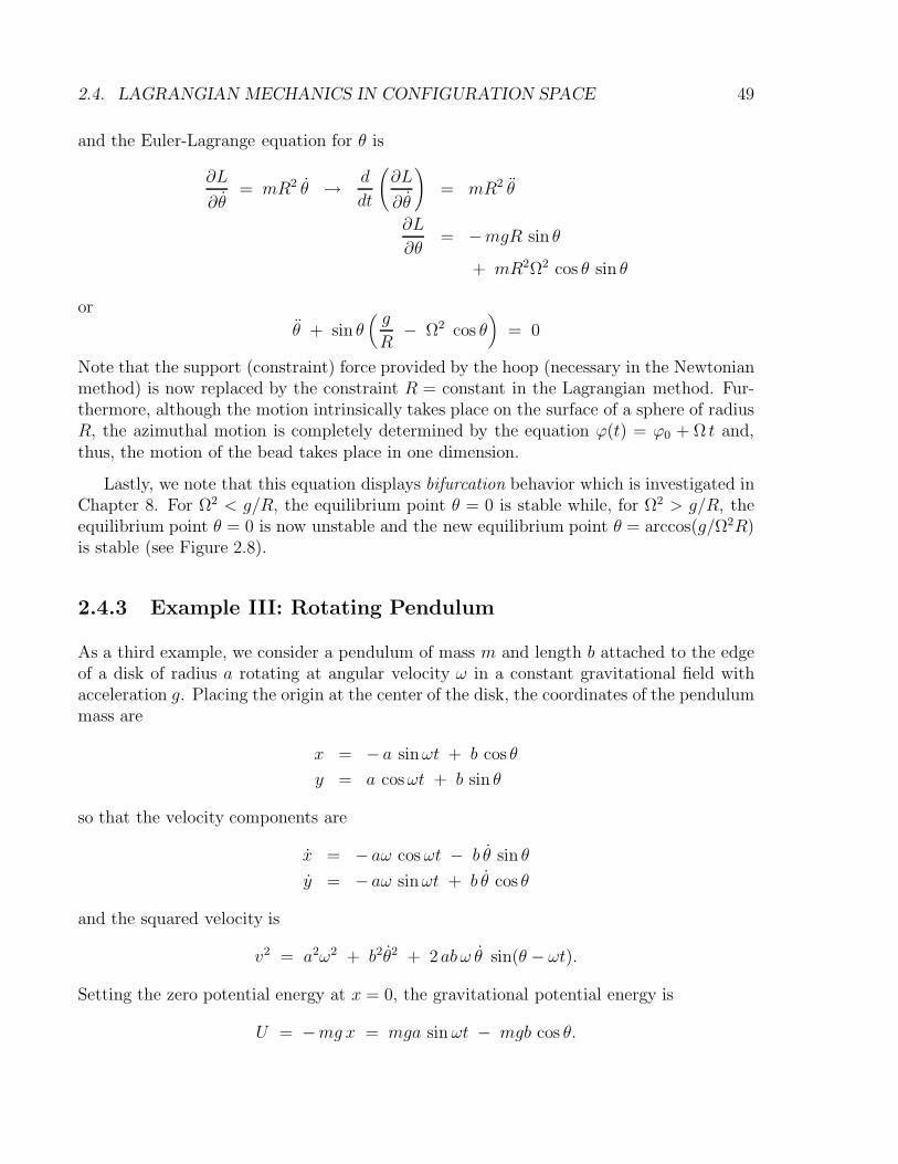
2.4. LAGRANGIAN MECHANICS IN CONFIGURATION SPACE 49
and the Euler-Lagrange equation for θ is
∂L
∂θ= mR2 θ → d
dt
(∂L
∂θ
)
= mR2 θ
∂L
∂θ= −mgR sin θ
+ mR2Ω2 cos θ sin θ
or
θ + sin θ(g
R− Ω2 cos θ
)= 0
Note that the support (constraint) force provided by the hoop (necessary in the Newtonianmethod) is now replaced by the constraint R = constant in the Lagrangian method. Fur-thermore, although the motion intrinsically takes place on the surface of a sphere of radiusR, the azimuthal motion is completely determined by the equation ϕ(t) = ϕ0 + Ω t and,thus, the motion of the bead takes place in one dimension.
Lastly, we note that this equation displays bifurcation behavior which is investigated inChapter 8. For Ω2 < g/R, the equilibrium point θ = 0 is stable while, for Ω2 > g/R, theequilibrium point θ = 0 is now unstable and the new equilibrium point θ = arccos(g/Ω2R)is stable (see Figure 2.8).
2.4.3 Example III: Rotating Pendulum
As a third example, we consider a pendulum of mass m and length b attached to the edgeof a disk of radius a rotating at angular velocity ω in a constant gravitational field withacceleration g. Placing the origin at the center of the disk, the coordinates of the pendulummass are
x = − a sinωt + b cos θ
y = a cosωt + b sin θ
so that the velocity components are
x = − aω cosωt − b θ sin θ
y = − aω sinωt + b θ cos θ
and the squared velocity is
v2 = a2ω2 + b2θ2 + 2ab ω θ sin(θ − ωt).
Setting the zero potential energy at x = 0, the gravitational potential energy is
U = −mg x = mga sinωt − mgb cos θ.
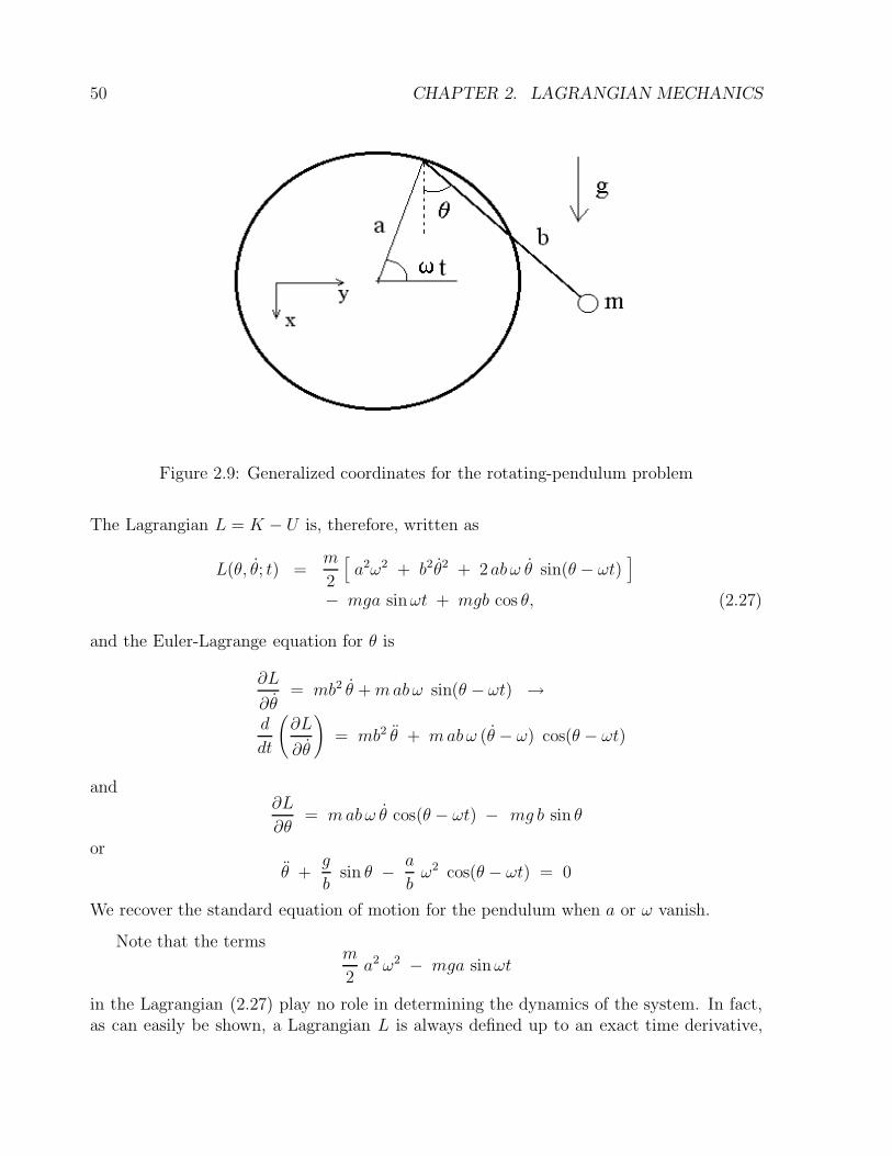
50 CHAPTER 2. LAGRANGIAN MECHANICS
Figure 2.9: Generalized coordinates for the rotating-pendulum problem
The Lagrangian L = K − U is, therefore, written as
L(θ, θ; t) =m
2
[a2ω2 + b2θ2 + 2ab ω θ sin(θ − ωt)
]
− mga sinωt + mgb cos θ, (2.27)
and the Euler-Lagrange equation for θ is
∂L
∂θ= mb2 θ +mabω sin(θ − ωt) →
d
dt
(∂L
∂θ
)
= mb2 θ + mabω (θ − ω) cos(θ − ωt)
and∂L
∂θ= mabω θ cos(θ − ωt) − mg b sin θ
or
θ +g
bsin θ − a
bω2 cos(θ − ωt) = 0
We recover the standard equation of motion for the pendulum when a or ω vanish.
Note that the termsm
2a2 ω2 − mga sinωt
in the Lagrangian (2.27) play no role in determining the dynamics of the system. In fact,as can easily be shown, a Lagrangian L is always defined up to an exact time derivative,
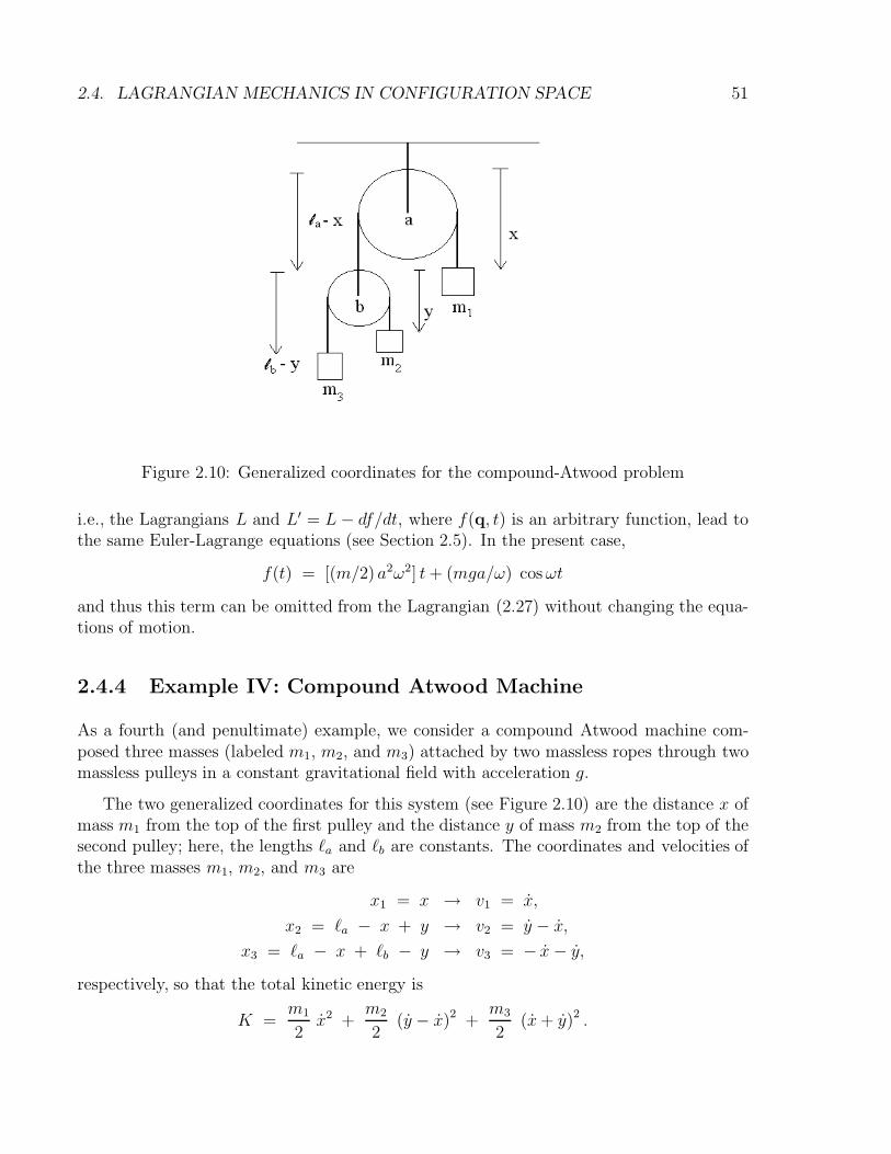
2.4. LAGRANGIAN MECHANICS IN CONFIGURATION SPACE 51
Figure 2.10: Generalized coordinates for the compound-Atwood problem
i.e., the Lagrangians L and L′ = L − df/dt, where f(q, t) is an arbitrary function, lead tothe same Euler-Lagrange equations (see Section 2.5). In the present case,
f(t) = [(m/2) a2ω2] t+ (mga/ω) cosωt
and thus this term can be omitted from the Lagrangian (2.27) without changing the equa-tions of motion.
2.4.4 Example IV: Compound Atwood Machine
As a fourth (and penultimate) example, we consider a compound Atwood machine com-posed three masses (labeled m1, m2, and m3) attached by two massless ropes through twomassless pulleys in a constant gravitational field with acceleration g.
The two generalized coordinates for this system (see Figure 2.10) are the distance x ofmass m1 from the top of the first pulley and the distance y of mass m2 from the top of thesecond pulley; here, the lengths `a and `b are constants. The coordinates and velocities ofthe three masses m1, m2, and m3 are
x1 = x → v1 = x,
x2 = `a − x + y → v2 = y − x,
x3 = `a − x + `b − y → v3 = − x− y,
respectively, so that the total kinetic energy is
K =m1
2x2 +
m2
2(y − x)2 +
m3
2(x+ y)2 .
52 CHAPTER 2. LAGRANGIAN MECHANICS
Placing the zero potential energy at the top of the first pulley, the total gravitationalpotential energy, on the other hand, can be written as
U = − g x (m1 −m2 −m3) − g y (m2 −m3) ,
where constant terms were omitted. The Lagrangian L = K − U is, therefore, written as
L(x, x, y, y) =m1
2x2 +
m2
2(x− y)
2+
m3
2(x+ y)
2
+ g x (m1 −m2 −m3) + g y (m2 −m3) .
The Euler-Lagrange equation for x is
∂L
∂x= (m1 +m2 +m3) x+ (m3 −m2) y →
d
dt
(∂L
∂x
)
= (m1 +m2 +m3) x+ (m3 −m2) y
∂L
∂x= g (m1 −m2 −m3)
while the Euler-Lagrange equation for y is
∂L
∂y= (m3 −m2) x + (m2 +m3) y →
d
dt
(∂L
∂y
)
= (m3 −m2) x + (m2 +m3) y
∂L
∂y= g (m2 −m3) .
We combine these two Euler-Lagrange equations
(m1 +m2 +m3) x+ (m3 −m2) y = g (m1 −m2 −m3) , (2.28)
(m3 −m2) x + (m2 +m3) y = g (m2 −m3) , (2.29)
to describe the dynamical evolution of the Compound Atwood Machine. This set of equa-tions can, in fact, be solved explicitly as
x = g
(m1m+ − (m2
+ −m2−)
m1m+ + (m2+ −m2
−)
)
and y = g
(2 m1m−
m1m+ + (m2+ −m2
−)
)
,
where m± = m2 ±m3. Note also that, by using the energy conservation law E = K + Uit can be shown that the position z of the center of mass of the mechanical system (asmeasured from the top of the first pulley) satisfies the relation
Mg (z − z0) =m1
2x2 +
m2
2(y − x)2 +
m3
2(x+ y)2 > 0, (2.30)
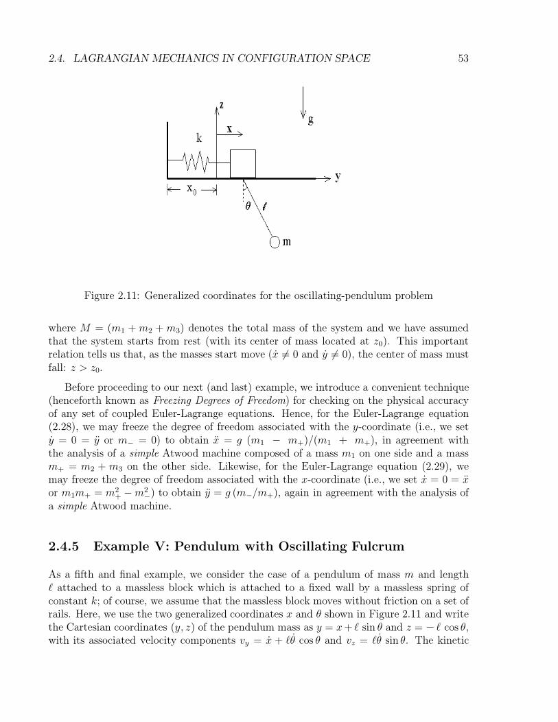
2.4. LAGRANGIAN MECHANICS IN CONFIGURATION SPACE 53
Figure 2.11: Generalized coordinates for the oscillating-pendulum problem
where M = (m1 + m2 + m3) denotes the total mass of the system and we have assumedthat the system starts from rest (with its center of mass located at z0). This importantrelation tells us that, as the masses start move (x 6= 0 and y 6= 0), the center of mass mustfall: z > z0.
Before proceeding to our next (and last) example, we introduce a convenient technique(henceforth known as Freezing Degrees of Freedom) for checking on the physical accuracyof any set of coupled Euler-Lagrange equations. Hence, for the Euler-Lagrange equation(2.28), we may freeze the degree of freedom associated with the y-coordinate (i.e., we sety = 0 = y or m− = 0) to obtain x = g (m1 − m+)/(m1 + m+), in agreement withthe analysis of a simple Atwood machine composed of a mass m1 on one side and a massm+ = m2 + m3 on the other side. Likewise, for the Euler-Lagrange equation (2.29), wemay freeze the degree of freedom associated with the x-coordinate (i.e., we set x = 0 = xor m1m+ = m2
+ −m2−) to obtain y = g (m−/m+), again in agreement with the analysis of
a simple Atwood machine.
2.4.5 Example V: Pendulum with Oscillating Fulcrum
As a fifth and final example, we consider the case of a pendulum of mass m and length` attached to a massless block which is attached to a fixed wall by a massless spring ofconstant k; of course, we assume that the massless block moves without friction on a set ofrails. Here, we use the two generalized coordinates x and θ shown in Figure 2.11 and writethe Cartesian coordinates (y, z) of the pendulum mass as y = x+ ` sin θ and z = − ` cos θ,with its associated velocity components vy = x + `θ cos θ and vz = `θ sin θ. The kinetic

54 CHAPTER 2. LAGRANGIAN MECHANICS
energy of the pendulum is thus
K =m
2
(v2y + v2
z
)=
m
2
(x2 + `2θ2 + 2 ` cos θ xθ
).
The potential energy U = Uk + Ug has two terms: one term Uk = 12kx2 associated with
displacement of the spring away from its equilibrium position and one term Ug = mgzassociated with gravity. Hence, the Lagrangian for this system is
L(x, θ, x, θ) =m
2
(x2 + `2θ2 + 2 ` cos θ xθ
)− k
2x2 + mg` cos θ.
The Euler-Lagrange equation for x is
∂L
∂x= m
(x + ` cos θ θ
)→
d
dt
(∂L
∂x
)
= m x + m`(θ cos θ − θ2 sin θ
)
∂L
∂x= − k x
while the Euler-Lagrange equation for θ is
∂L
∂θ= m`
(` θ + x cos θ
)→
d
dt
(∂L
∂θ
)
= m`2 θ + m`(x cos θ − xθ sin θ
)
∂L
∂θ= − m` xθ sin θ − mg` sin θ
or
m x + k x = m`(θ2 sin θ − θ cos θ
), (2.31)
θ + (g/`) sin θ = − (x/`) cos θ. (2.32)
Here, we recover the dynamical equation for a block-and-spring harmonic oscillator fromEq. (2.31) by freezing the degree of freedom associated with the θ-coordinate (i.e., by settingθ = 0 = θ) and the dynamical equation for the pendulum from Eq. (2.32) by freezing thedegree of freedom associated with the x-coordinate (i.e., by setting x = 0 = x). It iseasy to see from this last example how powerful and yet simple the Lagrangian method iscompared to the Newtonian method.
2.5. SYMMETRIES AND CONSERVATION LAWS 55
Numerical Box
By introducing the frequencies ωk =√k/m and ωg =
√g/`, with Ω ≡ ωk/ωg and d/dt =
ωg d/dτ , the coupled equations (2.31) and (2.32) are now expressed in dimensionless formas
s′′ + Ω2 s = (θ′)2 sin θ − θ′′ cos θ
θ′′ + sin θ = − s′′ cos θ,
where a prime denotes a derivative with respect to the dimensionless time τ = ωgt ands = x/` denotes the dimensionless displacement of the spring. Note that these coupledequations now involve the single parameter Ω, where Ω 1 represents the weak-springlimit while Ω 1 represents the strong-spring limit.
2.5 Symmetries and Conservation Laws
We are sometimes faced with a Lagrangian function that is either independent of time,independent of a linear spatial coordinate, or independent of an angular spatial coordinate.The Noether theorem (Amalie Emmy Noether, 1882-1935) states that for each symmetry ofthe Lagrangian there corresponds a conservation law (and vice versa). When the LagrangianL is invariant under a time translation, a space translation, or a spatial rotation, theconservation law involves energy, linear momentum, or angular momentum, respectively.
We begin our discussion with a general expression for the variation δL of the LagrangianL(q, q, t):
δL = δq ·
[∂L
∂q− d
dt
(∂L
∂q
) ]
+d
dt
(
δq ·∂L
∂q
)
,
obtained after re-arranging the term δq · ∂L/∂q. Next, we make use of the Euler-Lagrangeequations for q (which enables us to drop the term δq · [· · ·]) and we find
δL =d
dt
(
δq ·∂L
∂q
)
. (2.33)
Lastly, the variation δL can only be generated by a time translation δt, since
0 = δ∫L dt =
∫ [ (
δL + δt∂L
∂t
)
dt + L dδt
]
=∫ [
δL − δt
(dL
dt− ∂L
∂t
) ]
dt
56 CHAPTER 2. LAGRANGIAN MECHANICS
so that
δL = δt
(dL
dt− ∂L
∂t
)
By combining this expression with Eq. (2.33), we find
δt
(dL
dt− ∂L
∂t
)
=d
dt
(
δq ·∂L
∂q
)
, (2.34)
which we, henceforth, refer to as the Noether equation for finite-dimensional mechanicalsystems [see Eq. (9.10) in Chapter 9 for the infinite-dimensional case].
We now apply Noether’s Theorem, based on the Noether equation (2.34), to investigatethe connection between symmetries of the Lagrangian with conservation laws.
2.5.1 Energy Conservation Law
First, we consider time translations, t→ t+δt and δq = q δt, so that the Noether equation(2.34) becomes Euler’s Second Equation for the Lagrangian:
− ∂L
∂t=
d
dt
(
q ·∂L
∂q− L
)
.
Noether’s Theorem states that if the Lagrangian is invariant under time translations, i.e.,∂L/∂t = 0, then energy is conserved, dE/dt = 0, where
E = q ·∂L
∂q− L
defines the energy invariant.
2.5.2 Momentum Conservation Laws
Next, we consider invariance under spatial translations, q → q+ε (where δq = ε denotes aconstant infinitesimal displacement and δt = 0), so that the Noether equation (2.34) yieldsthe linear momentum conservation law
0 =d
dt
(∂L
∂q
)
=dP
dt,
where P denotes the total linear momentum of the mechanical system. On the otherhand, when the Lagrangian is invariant under spatial rotations, q → q + (δϕ×q) (whereδϕ = δϕ ϕ denotes a constant infinitesimal rotation about an axis along the ϕ-direction),the Noether equation (2.34) yields the angular momentum conservation law
0 =d
dt
(
q×∂L
∂q
)
=dL
dt,
where L = q×P denotes the total angular momentum of the mechanical system.
2.5. SYMMETRIES AND CONSERVATION LAWS 57
2.5.3 Invariance Properties of a Lagrangian
Lastly, an important invariance property of the Lagrangian is related to the fact that theEuler-Lagrange equations themselves are invariant under the gauge transformation
L → L +dF
dt(2.35)
on the Lagrangian itself, where F (q, t) is an arbitrary time-dependent function so that
dF (q, t)
dt=
∂F
∂t+∑
j
qj∂F
∂qj.
To investigate the invariance property (2.35), we call L′ = L + dF/dt the new Lagrangianand L the old Lagrangian, and consider the new Euler-Lagrange equations
d
dt
(∂L′
∂qi
)
=∂L′
∂qi.
We now express each term in terms of the old Lagrangian L and the function F . Let usbegin with
∂L′
∂qi=
∂
∂qi
L +∂F
∂t+∑
j
qj∂F
∂qj
=∂L
∂qi+
∂F
∂qi,
so thatd
dt
(∂L′
∂qi
)
=d
dt
(∂L
∂qi
)
+∂2F
∂t∂qi+∑
k
qk∂2F
∂qk∂qi.
Next, we find
∂L′
∂qi=
∂
∂qi
L +∂F
∂t+∑
j
qj∂F
∂qj
=∂L
∂qi+
∂2F
∂qi∂t+∑
j
qj∂2F
∂qi∂qj.
Using the symmetry properties
qj∂2F
∂qi∂qj= qj
∂2F
∂qj∂qiand
∂2F
∂t∂qi=
∂2F
∂qi∂t,
we easily verify that
d
dt
(∂L′
∂qi
)
− ∂L′
∂qi=
d
dt
(∂L
∂qi
)
− ∂L
∂qi= 0.
Hence, since L and L′ = L + dF/dt lead to the same Euler-Lagrange equations, they aresaid to be equivalent.

58 CHAPTER 2. LAGRANGIAN MECHANICS
Using this invariance property, for example, we note that the Lagrangian is also invariantunder the Galilean velocity transformation v → v + α, so that the Lagrangian variation
δL = α ·
(
v∂L
∂v2
)
≡ α ·dx
dt
∂L
∂v2,
using the kinetic identity ∂L/∂v2 = m/2, can be written as an exact time derivative
δL =d
dt
(α ·
m
2x
)≡ dδF
dt.
Hence, because Lagrangian mechanics is invariant under the gauge transformation (2.35),the Lagrangian L is said to be Galilean invariant.
2.5.4 Lagrangian Mechanics with Symmetries
As an example of Lagrangian mechanics with symmetries, we return to the motion of aparticle of mass m constrained to move on the surface of a cone of apex angle α (such that√x2 + y2 = z tanα) in the presence of a gravitational field (see Figure 2.5 and Sec. 2.3.3).
The Lagrangian for this constrained mechanical system is expressed in terms of thegeneralized coordinates (s, θ), where s denotes the distance from the cone’s apex (labeled Oin Figure 2.5) and θ is the standard polar angle in the (x, y)-plane. Hence, by combining thekinetic energy K = 1
2m(s2+s2 θ2 sin2 α) with the potential energy U = mgz = mg s cosα,
we construct the Lagrangian
L(s, θ; s, θ) =1
2m(s2 + s2 θ2 sin2 α
)− mg s cosα. (2.36)
Since the Lagrangian is independent of the polar angle θ, the canonical angular momentum
pθ =∂L
∂θ= ms2 θ sin2 α (2.37)
is a constant of the motion (as predicted by Noether’s Theorem). The Euler-Lagrangeequation for s, on the other hand, is expressed as
s + g cosα = s θ2 sin2 α =p2θ
m2 s3 sin2 α, (2.38)
where g cosα denotes the component of the gravitational acceleration parallel to the surfaceof the cone. The right side of Eq. (2.38) involves s only after using θ = pθ/(ms2 sin2 α),which follows from the conservation of angular momentum.
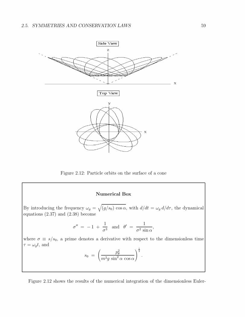
2.5. SYMMETRIES AND CONSERVATION LAWS 59
Figure 2.12: Particle orbits on the surface of a cone
Numerical Box
By introducing the frequency ωg =√
(g/s0) cosα, with d/dt = ωg d/dτ , the dynamical
equations (2.37) and (2.38) become
σ′′ = − 1 +1
σ3and θ′ =
1
σ2 sinα,
where σ ≡ s/s0, a prime denotes a derivative with respect to the dimensionless timeτ = ωgt, and
s0 =
(p2θ
m2g sin2 α cosα
) 1
3
.
Figure 2.12 shows the results of the numerical integration of the dimensionless Euler-
60 CHAPTER 2. LAGRANGIAN MECHANICS
Lagrange equations for θ(τ ) and σ(τ ); see Numerical Box. The top figure in Figure 2.12shows a projection of the path of the particle on the (x, z)-plane (side view), which clearlyshows that the motion is periodic as the σ-coordinate oscillates between two finite valuesof σ. The bottom figure in Figure 2.12 shows a projection of the path of the particle onthe (x, y)-plane (top view), which shows the slow precession motion in the θ-coordinate. Inthe next Chapter, we will show that the doubly-periodic motion of the particle moving onthe surface of the inverted cone is a result of the conservation law of angular momentumand energy (since the Lagrangian system is also independent of time).
2.5.5 Routh’s Procedure for Eliminating Ignorable Coordinates
Edward John Routh (1831-1907) introduced a simple procedure for eliminating ignorabledegrees of freedom while introducing their corresponding conserved momenta. Consider,for example, two-dimensional motion on the (x, y)-plane represented by the LagrangianL(r; r, θ), where r and θ are the polar coordinates. Since the Lagrangian under consid-eration is independent of the angle θ, the canonical momentum pθ = ∂L/∂θ is conserved.Routh’s procedure for deriving a reduced Lagrangian involves the construction of the Routh-Lagrange function (or Routhian) R(r, r; pθ) defined as
R(r, r; pθ) = L(r; r, θ) − pθ θ, (2.39)
where θ is expressed as a function of r and pθ.
For example, for the constrained motion of a particle on the surface of a cone in the pres-ence of gravity, the Lagrangian (2.36) can be reduced to the Routh-Lagrange (or Routhian)function
R(s, s; pθ) =1
2ms2 −
(
mg s cosα +p2θ
2ms2 sin2 α
)
=1
2ms2 − V (s), (2.40)
and the equation of motion (2.38) can be expressed in Euler-Lagrange form
d
ds
(∂R
∂s
)
=∂R
∂s→ m s = − V ′(s),
in terms of the effective potential
V (s) = mg s cosα +p2θ
2ms2 sin2 α.
Here, the effective potential V (s) has a single minimum at s = s0, where
s0 =
(p2θ
m2g sin2 α cosα
)1
3
and V0 ≡ V (s0) = 32mg s0 cosα.
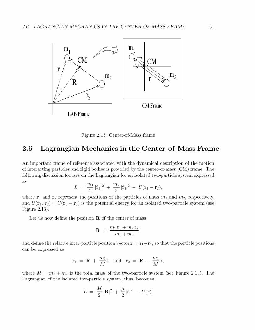
2.6. LAGRANGIAN MECHANICS IN THE CENTER-OF-MASS FRAME 61
Figure 2.13: Center-of-Mass frame
2.6 Lagrangian Mechanics in the Center-of-Mass Frame
An important frame of reference associated with the dynamical description of the motionof interacting particles and rigid bodies is provided by the center-of-mass (CM) frame. Thefollowing discussion focuses on the Lagrangian for an isolated two-particle system expressedas
L =m1
2|r1|2 +
m2
2|r2|2 − U(r1 − r2),
where r1 and r2 represent the positions of the particles of mass m1 and m2, respectively,and U(r1, r2) = U(r1 − r2) is the potential energy for an isolated two-particle system (seeFigure 2.13).
Let us now define the position R of the center of mass
R =m1 r1 +m2 r2
m1 +m2,
and define the relative inter-particle position vector r = r1−r2, so that the particle positionscan be expressed as
r1 = R +m2
Mr and r2 = R − m1
Mr,
where M = m1 + m2 is the total mass of the two-particle system (see Figure 2.13). TheLagrangian of the isolated two-particle system, thus, becomes
L =M
2|R|2 +
µ
2|r|2 − U(r),
62 CHAPTER 2. LAGRANGIAN MECHANICS
where
µ =m1m2
m1 +m2
=(
1
m1
+1
m2
)−1
denotes the reduced mass of the two-particle system. We note that the angular momentumof the two-particle system is expressed as
L =∑
a
ra ×pa = R×P + r×p, (2.41)
where the canonical momentum of the center-of-mass P and the canonical momentum p
of the two-particle system in the CM frame are defined, respectively, as
P =∂L
∂R= M R and p =
∂L
∂r= µr.
For an isolated system (∂L/∂R = 0), the canonical momentum P of the center-of-mass isa constant of the motion. The CM reference frame is defined by the condition R = 0, i.e.,we move the origin of our coordinate system to the CM position.
In the CM frame, the Lagrangian for an isolated two-particle system is
L(r, r) =µ
2|r|2 − U(r), (2.42)
which describes the motion of a fictitious particle of mass µ at position r, where the positionsof the two real particles of masses m1 and m2 are
r1 =m2
Mr and r2 = − m1
Mr. (2.43)
Hence, once the Euler-Lagrange equation for r
d
dt
(∂L
∂r
)
=∂L
∂r→ µ r = −∇U(r)
is solved, the motion of the two particles in the CM frame is determined through Eqs. (2.43).
The angular momentum L = µ r× r in the CM frame satisfies the evolution equation
dL
dt= r×µr = − r×∇U(r). (2.44)
Here, using spherical coordinates (r, θ, ϕ), we find
dL
dt= − ϕ
∂U
∂θ+
θ
sin θ
∂U
∂ϕ.
If motion is originally taking place on the (x, y)-plane (i.e., at θ = π/2) and the potentialU(r, ϕ) is independent of the polar angle θ, then the angular momentum vector is L = ` z
and its magnitude ` satisfies the evolution equation
d`
dt= − ∂U
∂ϕ.
2.6. LAGRANGIAN MECHANICS IN THE CENTER-OF-MASS FRAME 63
Hence, for motion in a potential U(r) that depends only on the radial position r, theangular momentum remains along the z-axis L = ` z represents an additional constant ofmotion. Motion in such potentials is refered to as motion in a central-force potential andwill be studied in Chap. 4.
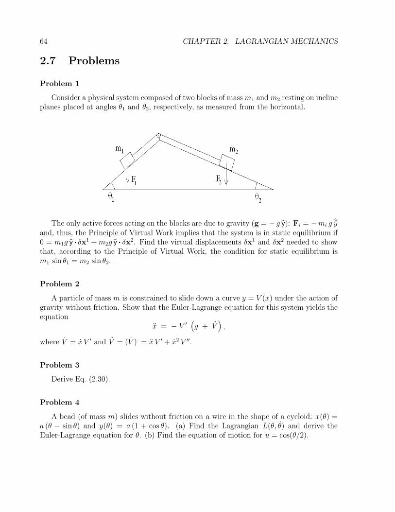
64 CHAPTER 2. LAGRANGIAN MECHANICS
2.7 Problems
Problem 1
Consider a physical system composed of two blocks of mass m1 and m2 resting on inclineplanes placed at angles θ1 and θ2, respectively, as measured from the horizontal.
The only active forces acting on the blocks are due to gravity (g = − g y): Fi = −mi g yand, thus, the Principle of Virtual Work implies that the system is in static equilibrium if0 = m1g y · δx1 +m2g y · δx2. Find the virtual displacements δx1 and δx2 needed to showthat, according to the Principle of Virtual Work, the condition for static equilibrium ism1 sin θ1 = m2 sin θ2.
Problem 2
A particle of mass m is constrained to slide down a curve y = V (x) under the action ofgravity without friction. Show that the Euler-Lagrange equation for this system yields theequation
x = − V ′(g + V
),
where V = x V ′ and V = (V )· = x V ′ + x2 V ′′.
Problem 3
Derive Eq. (2.30).
Problem 4
A bead (of mass m) slides without friction on a wire in the shape of a cycloid: x(θ) =a (θ − sin θ) and y(θ) = a (1 + cos θ). (a) Find the Lagrangian L(θ, θ) and derive theEuler-Lagrange equation for θ. (b) Find the equation of motion for u = cos(θ/2).
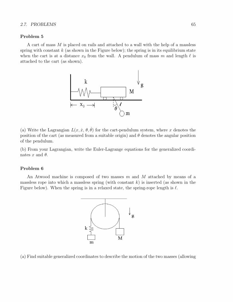
2.7. PROBLEMS 65
Problem 5
A cart of mass M is placed on rails and attached to a wall with the help of a masslessspring with constant k (as shown in the Figure below); the spring is in its equilibrium statewhen the cart is at a distance x0 from the wall. A pendulum of mass m and length ` isattached to the cart (as shown).
(a) Write the Lagrangian L(x, x, θ, θ) for the cart-pendulum system, where x denotes theposition of the cart (as measured from a suitable origin) and θ denotes the angular positionof the pendulum.
(b) From your Lagrangian, write the Euler-Lagrange equations for the generalized coordi-nates x and θ.
Problem 6
An Atwood machine is composed of two masses m and M attached by means of amassless rope into which a massless spring (with constant k) is inserted (as shown in theFigure below). When the spring is in a relaxed state, the spring-rope length is `.
(a) Find suitable generalized coordinates to describe the motion of the two masses (allowing
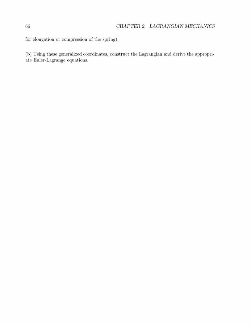
66 CHAPTER 2. LAGRANGIAN MECHANICS
for elongation or compression of the spring).
(b) Using these generalized coordinates, construct the Lagrangian and derive the appropri-ate Euler-Lagrange equations.
Chapter 3
Hamiltonian Mechanics
In the previous Chapter, the Lagrangian method was introduced as a powerful alternativeto the Newtonian method for deriving equations of motion for complex mechanical systems.In the present Chapter, a complementary approach to the Lagrangian method, known as theHamiltonian method, is presented. Although much of the Hamiltonian method is outsidethe scope of this course (e.g., the canonical and noncanonical Hamiltonian formulations ofClassical Mechanics and the Hamiltonian formulation of Quantum Mechanics), a simplifiedversion (the Energy method) is presented here as a practical method for solving the Euler-Lagrange equations by quadrature.
3.1 Canonical Hamilton’s Equations
The k second-order Euler-Lagrange equations on configuration space q = (q1, ..., qk)
d
dt
(∂L
∂qj
)
=∂L
∂qj, (3.1)
can be written as 2k first-order differential equations, known as Hamilton’s equations(William Rowan Hamilton, 1805-1865), on a 2k-dimensional phase space with coordinatesz = (q1, ..., qk; p1, ..., pk), where
pj(q, q; t) =∂L
∂qj(q, q; t) (3.2)
defines the jth-component of the canonical momentum. In terms of these new coordinates,the Euler-Lagrange equations (3.1) are transformed into Hamilton’s canonical equations
dqj
dt=
∂H
∂pjand
dpjdt
= − ∂H
∂qj, (3.3)
67
68 CHAPTER 3. HAMILTONIAN MECHANICS
where the Hamiltonian functionH(q,p; t) is defined from the Lagrangian function L(q, q; t)by the Legendre transformation (Adrien-Marie Legendre, 1752-1833)
H(q,p; t) = p · q(q,p, t) − L[q, q(q,p, t), t]. (3.4)
We note that Hamilton’s equations (3.3) can also be derived from a variational principleas follows. First, we use the inverse of the Legendre transformation
L(z, z; t) = p · q −H(z; t) (3.5)
to obtain an expression for the Lagrangian function in phase space. Next, we calculate thefirst-variation of the action integral
δ∫L(q,p; t) dt =
∫ [
δp ·
(
q − ∂H
∂p
)
+
(
p · δq − δq ·∂H
∂q
) ]
dt,
where the variations δqi and δpi are now considered independent (and they are both as-sumed to vanish at the end points). Lastly, by integrating by parts the term p · δq, wefind
δ∫
L(q,p; t) dt =∫ [
δp ·
(
q − ∂H
∂p
)
− δq ·
(
p +∂H
∂q
) ]
dt,
so that the Principle of Least Action∫δLdt = 0 now yields Hamilton’s equations (3.3).
3.2 Legendre Transformation*
Before proceeding with the Hamiltonian formulation of particle dynamics, we investigatethe conditions under which the Legendre transformation (3.4) is possible. It turns out thatthe condition under which the Legendre transformation can be used is associated with thecondition under which the inversion of the relation p(r, r, t) → r(r,p, t) is possible. Tosimplify our discussion, we focus on motion in two dimensions (labeled x and y).
The general expression of the kinetic energy term of a Lagrangian with two degrees offreedom L(x, x, y, y) = K(x, x, y, y) − U(x, y) is
K(x, x, y, y) =α
2x2 + β x y +
γ
2y2 =
1
2rT · M · r, (3.6)
where r> = (x, y) denotes the transpose of r (see Appendix A for additional details con-cerning linear algebra) and the mass matrix M is
M =
α β
β γ
.
3.2. LEGENDRE TRANSFORMATION* 69
Here, the coefficients α, β, and γ may be function of x and/or y. The canonical momentumvector (3.2) is thus defined as
p =∂L
∂r= M · r →
px
py
=
α β
β γ
·
x
y
orpx = α x + β y
py = β x + γ y
. (3.7)
The Lagrangian is said to be regular if the matrix M is invertible, i.e., if its determinant
∆ = α γ − β2 6= 0.
In the case of a regular Lagrangian, we readily invert (3.7) to obtain
r(r,p, t) = M−1 · p →
x
y
=1
∆
γ − β
− β α
·
px
py
orx = (γ px − β py)/∆
y = (αpy − β px)/∆
, (3.8)
and the kinetic energy term becomes
K(x, px, y, py) =1
2p> · M−1 · p.
Lastly, under the Legendre transformation, we find
H = p> ·(M−1 · p
)−(
1
2p> · M−1 · p − U
)
=1
2p> · M−1 · p + U.
Hence, we clearly see that the Legendre transformation is applicable only if the mass matrixM in the kinetic energy (3.6) is invertible.
Lastly, we note that the Legendre transformation is also used in other areas in physicssuch as Thermodynamics. Indeed, we begin with the First Law of Thermodynamics
dU(S, V ) = T dS − P dV
expressed in terms of the internal energy function U(S, V ), where entropy S and volume Vare the independent variables while temperature T (S, V ) = ∂U/∂S and pressure P (S, V ) =
70 CHAPTER 3. HAMILTONIAN MECHANICS
− ∂U/∂V are dependent variables. It is possible, however, to choose other independentvariables by defining new thermodynamic functions as shown in the Table below.
Pressure P Volume V Temperature T Entropy S
Pressure P × × G = H − T S H = U + P VVolume V × × F = U − T S U
Temperature T G = H − T S F = U − T S × ×Entropy S H = U + P V U × ×
For example, if we choose volume V and temperature T as independent variables, weintroduce the Legendre transformation from the internal energy U(S, V ) to the Helmholtzfree energy F (V, T ) = U − T S, such that the First Law of Thermodynamics now becomes
dF (V, T ) = dU − T dS − S dT = − P dV − S dT,
where pressure P (V, T ) = − ∂F/∂V and entropy S(V, T ) = − ∂F/∂T are dependent vari-ables. Likewise, enthalpy H(P, S) = U + P V and Gibbs free energy G(T, P ) = H − T Sare introduced by Legendre transformations whenever one chooses (P, S) and (T, P ), re-spectively, as independent variables.
3.3 Hamiltonian Optics and Wave-Particle Duality*
Historically, the Hamiltonian method was first introduced as a formulation of the dynamicsof light rays. Consider the following phase integral
Θ[z] =∫ t2
t1[ k · x − ω(x,k; t) ] dt, (3.9)
where Θ[z] is a functional of the light-path z(t) = (x(t), k(t)) in ray phase space, expressedin terms of the instantaneous position x(t) of a light ray and its associated instantaneouswave vector k(t); here, the dispersion relation ω(x,k; t) is obtained as a root of the disper-sion equation det D(x, t; k, ω) = 0, and a dot denotes a total time derivative: x = dx/dt.
Assuming that the phase integral Θ[z] acquires a minimal value for a physical ray orbitz(t), henceforth called the Principle of Phase Stationarity δΘ = 0, we can show that Euler’sFirst Equation leads to Hamilton’s ray equations:
dx
dt=
∂ω
∂kand
dk
dt= − ∇ω. (3.10)
The first ray equation states that a ray travels at the group velocity while the second rayequation states that the wave vector k is refracted as the ray propagates in a non-uniformmedium (see Chapter 1). Hence, the frequency function ω(x,k; t) is the Hamiltonian ofray dynamics in a nonuniform medium.
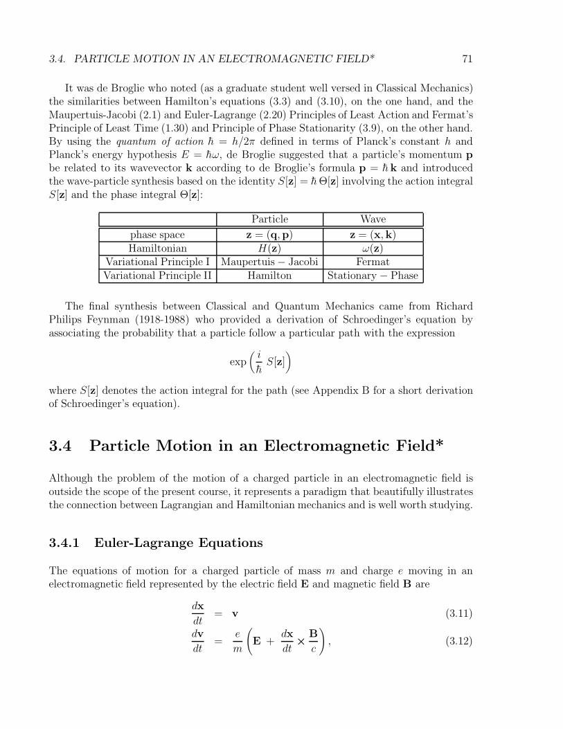
3.4. PARTICLE MOTION IN AN ELECTROMAGNETIC FIELD* 71
It was de Broglie who noted (as a graduate student well versed in Classical Mechanics)the similarities between Hamilton’s equations (3.3) and (3.10), on the one hand, and theMaupertuis-Jacobi (2.1) and Euler-Lagrange (2.20) Principles of Least Action and Fermat’sPrinciple of Least Time (1.30) and Principle of Phase Stationarity (3.9), on the other hand.By using the quantum of action h = h/2π defined in terms of Planck’s constant h andPlanck’s energy hypothesis E = hω, de Broglie suggested that a particle’s momentum p
be related to its wavevector k according to de Broglie’s formula p = h k and introducedthe wave-particle synthesis based on the identity S[z] = hΘ[z] involving the action integralS[z] and the phase integral Θ[z]:
Particle Wave
phase space z = (q,p) z = (x,k)Hamiltonian H(z) ω(z)
Variational Principle I Maupertuis − Jacobi FermatVariational Principle II Hamilton Stationary − Phase
The final synthesis between Classical and Quantum Mechanics came from RichardPhilips Feynman (1918-1988) who provided a derivation of Schroedinger’s equation byassociating the probability that a particle follow a particular path with the expression
exp(i
hS[z]
)
where S[z] denotes the action integral for the path (see Appendix B for a short derivationof Schroedinger’s equation).
3.4 Particle Motion in an Electromagnetic Field*
Although the problem of the motion of a charged particle in an electromagnetic field isoutside the scope of the present course, it represents a paradigm that beautifully illustratesthe connection between Lagrangian and Hamiltonian mechanics and is well worth studying.
3.4.1 Euler-Lagrange Equations
The equations of motion for a charged particle of mass m and charge e moving in anelectromagnetic field represented by the electric field E and magnetic field B are
dx
dt= v (3.11)
dv
dt=
e
m
(
E +dx
dt×
B
c
)
, (3.12)

72 CHAPTER 3. HAMILTONIAN MECHANICS
where x denotes the position of the particle and v its velocity.1
By treating the coordinates (x,v) as generalized coordinates (i.e., δv is treated inde-pendently from δx), we can show that the equations of motion (3.11) and (3.12) can beobtained as Euler-Lagrange equations from the Lagrangian (3.5)
L(x, x, v, v; t) =(mv +
e
cA(x, t)
)· x −
(eΦ(x, t) +
m
2|v|2
), (3.13)
where Φ and A are the electromagnetic potentials in terms of which electric and magneticfields are defined
E = −∇Φ − 1
c
∂A
∂tand B = ∇×A. (3.14)
Note that these expressions for E and B satisfy Faraday’s law ∇×E = − c−1 ∂B/∂t andthe divergenceless property ∇ ·B = 0 of the magnetic field.
First, we look at the Euler-Lagrange equation for x:
∂L
∂x= mv +
e
cA → d
dt
(∂L
∂x
)
= m v +e
c
(∂A
∂t+ x ·∇A
)
∂L
∂x=
e
c∇A · x − e∇Φ,
which yields Eq. (3.12), since
m v = − e
(
∇Φ +1
c
∂A
∂t
)
+e
cx×∇×A = eE +
e
cx×B, (3.15)
where the definitions (3.14) were used.
Next, we look at the Euler-Lagrange equation for v:
∂L
∂v= 0 → d
dt
(∂L
∂v
)
= 0 =∂L
∂v= m x − mv,
which yields Eq. (3.11). Because ∂L/∂v = 0, we note that we could use Eq. (3.11) as aconstraint which could be imposed a priori on the Lagrangian (3.13) to give
L(x, x; t) =m
2|x|2 +
e
cA(x, t) · x − eΦ(x, t). (3.16)
The Euler-Lagrange equation for x in this case is identical to Eq. (3.15) with v = x.
1Gaussian units are used whenever electromagnetic fields are involved.
3.4. PARTICLE MOTION IN AN ELECTROMAGNETIC FIELD* 73
3.4.2 Energy Conservation Law
We now show that the second Euler equation (i.e., the energy conservation law), expressedas
d
dt
(
L − x ·∂L
∂x
)
=∂L
∂t,
is satisfied exactly by the Lagrangian (3.16) and the equations of motion (3.11) and (3.12).First, from the Lagrangian (3.16), we find
∂L
∂t=
e
c
∂A
∂t·v − e
∂Φ
∂t
L − x ·∂L
∂x= L −
(mv +
e
cA
)·v
= −(m
2|v|2 + eΦ
).
Next, we find
d
dt
(
L − x ·∂L
∂x
)
= − mv · v − e
(∂Φ
∂t+ v ·∇Φ
)
= −e ∂
∂t
(Φ − v
c·A
).
Using Eq. (3.11), we readily find mv · v = eE ·v and thus
− eE ·v − e
(∂Φ
∂t+ v ·∇Φ
)
=e
c
∂A
∂t· v − e
∂Φ
∂t,
which is shown to be satisfied exactly by substituting the definition (3.14) for E.
3.4.3 Gauge Invariance
The electric and magnetic fields defined in (3.14) are invariant under the gauge transfor-mation
Φ → Φ − 1
c
∂χ
∂tand A → A + ∇χ, (3.17)
where χ(x, t) is an arbitrary scalar field. Although the equations of motion (3.11) and (3.12)are manifestly gauge invariant, the Lagrangian (3.16) is not manifestly gauge invariant sincethe electromagnetic potentials Φ and A appear explicitly. Under a gauge transformation(3.17), however, we find
L → L +e
cx ·∇χ − e
(
− 1
c
∂χ
∂t
)
= L +d
dt
(e
cχ).
Since Lagrangian Mechanics is invariant under the transformation (2.35), we find that theLagrangian (3.16) is invariant under a gauge transformation.
74 CHAPTER 3. HAMILTONIAN MECHANICS
3.4.4 Canonical Hamilton’s Equations
The canonical momentum p for a particle of mass m and charge e in an electromagneticfield is defined as
p(x,v, t) =∂L
∂x= mv +
e
cA(x, t). (3.18)
The canonical Hamiltonian function H(x,p, t) is now constructed through the Legendretransformation
H(x,p, t) = p · x(x,p, t) − L[x, x(x,p, t), t]
= eΦ(x, t) +1
2m
∣∣∣∣ p − e
cA(x, t)
∣∣∣∣2
, (3.19)
where v(x,p, t) was obtained by inverting p(x,v, t) from Eq. (3.18). Using the canonicalHamiltonian function (3.19), we immediately find
x =∂H
∂p=
1
m
(p − e
cA
),
p = − ∂H
∂x= − e ∇Φ − e
c∇A · x,
from which we recover the equations of motion (3.11) and (3.12) once we use the definition(3.18) for the canonical momentum.
3.5 One-degree-of-freedom Hamiltonian Dynamics
In this Section, we investigate Hamiltonian dynamics with one degree of freedom in a time-independent potential. In particular, we show that such systems are always integrable (i.e.,they can always be solved by quadrature).
The one degree-of-freedom Hamiltonian dynamics of a particle of mass m is based onthe Hamiltonian
H(x, p) =p2
2m+ U(x), (3.20)
where p = mx is the particle’s momentum and U(x) is the time-independent potentialenergy. The Hamilton’s equations (3.3) for this Hamiltonian are
dx
dt=
p
mand
dp
dt= − dU(x)
dx. (3.21)
Since the Hamiltonian (and Lagrangian) is time independent, the energy conservation lawstates that H(x, p) = E. In turn, this conservation law implies that the particle’s velocity
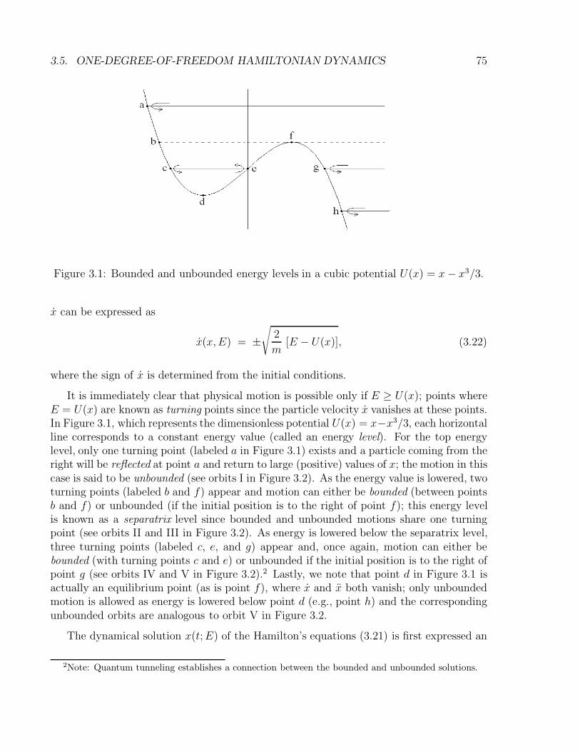
3.5. ONE-DEGREE-OF-FREEDOM HAMILTONIAN DYNAMICS 75
Figure 3.1: Bounded and unbounded energy levels in a cubic potential U(x) = x− x3/3.
x can be expressed as
x(x,E) = ±√
2
m[E − U(x)], (3.22)
where the sign of x is determined from the initial conditions.
It is immediately clear that physical motion is possible only if E ≥ U(x); points whereE = U(x) are known as turning points since the particle velocity x vanishes at these points.In Figure 3.1, which represents the dimensionless potential U(x) = x−x3/3, each horizontalline corresponds to a constant energy value (called an energy level). For the top energylevel, only one turning point (labeled a in Figure 3.1) exists and a particle coming from theright will be reflected at point a and return to large (positive) values of x; the motion in thiscase is said to be unbounded (see orbits I in Figure 3.2). As the energy value is lowered, twoturning points (labeled b and f) appear and motion can either be bounded (between pointsb and f) or unbounded (if the initial position is to the right of point f); this energy levelis known as a separatrix level since bounded and unbounded motions share one turningpoint (see orbits II and III in Figure 3.2). As energy is lowered below the separatrix level,three turning points (labeled c, e, and g) appear and, once again, motion can either bebounded (with turning points c and e) or unbounded if the initial position is to the right ofpoint g (see orbits IV and V in Figure 3.2).2 Lastly, we note that point d in Figure 3.1 isactually an equilibrium point (as is point f), where x and x both vanish; only unboundedmotion is allowed as energy is lowered below point d (e.g., point h) and the correspondingunbounded orbits are analogous to orbit V in Figure 3.2.
The dynamical solution x(t;E) of the Hamilton’s equations (3.21) is first expressed an
2Note: Quantum tunneling establishes a connection between the bounded and unbounded solutions.
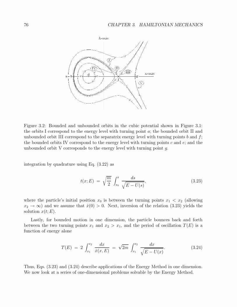
76 CHAPTER 3. HAMILTONIAN MECHANICS
Figure 3.2: Bounded and unbounded orbits in the cubic potential shown in Figure 3.1:the orbits I correspond to the energy level with turning point a; the bounded orbit II andunbounded orbit III correspond to the separatrix energy level with turning points b and f ;the bounded orbits IV correspond to the energy level with turning points c and e; and theunbounded orbit V corresponds to the energy level with turning point g.
integration by quadrature using Eq. (3.22) as
t(x;E) =
√m
2
∫ x
x0
ds√E − U(s)
, (3.23)
where the particle’s initial position x0 is between the turning points x1 < x2 (allowingx2 → ∞) and we assume that x(0) > 0. Next, inversion of the relation (3.23) yields thesolution x(t;E).
Lastly, for bounded motion in one dimension, the particle bounces back and forthbetween the two turning points x1 and x2 > x1, and the period of oscillation T (E) is afunction of energy alone
T (E) = 2∫ x2
x1
dx
x(x,E)=
√2m
∫ x2
x1
dx√E − U(x)
. (3.24)
Thus, Eqs. (3.23) and (3.24) describe applications of the Energy Method in one dimension.We now look at a series of one-dimensional problems solvable by the Energy Method.
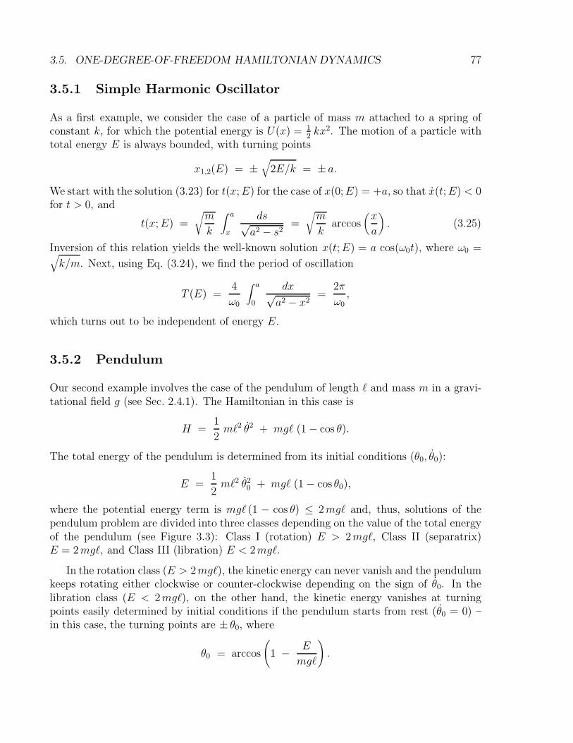
3.5. ONE-DEGREE-OF-FREEDOM HAMILTONIAN DYNAMICS 77
3.5.1 Simple Harmonic Oscillator
As a first example, we consider the case of a particle of mass m attached to a spring ofconstant k, for which the potential energy is U(x) = 1
2kx2. The motion of a particle with
total energy E is always bounded, with turning points
x1,2(E) = ±√
2E/k = ± a.
We start with the solution (3.23) for t(x;E) for the case of x(0;E) = +a, so that x(t;E) < 0for t > 0, and
t(x;E) =
√m
k
∫ a
x
ds√a2 − s2
=
√m
karccos
(x
a
). (3.25)
Inversion of this relation yields the well-known solution x(t;E) = a cos(ω0t), where ω0 =√k/m. Next, using Eq. (3.24), we find the period of oscillation
T (E) =4
ω0
∫ a
0
dx√a2 − x2
=2π
ω0,
which turns out to be independent of energy E.
3.5.2 Pendulum
Our second example involves the case of the pendulum of length ` and mass m in a gravi-tational field g (see Sec. 2.4.1). The Hamiltonian in this case is
H =1
2m`2 θ2 + mg` (1 − cos θ).
The total energy of the pendulum is determined from its initial conditions (θ0, θ0):
E =1
2m`2 θ2
0 + mg` (1 − cos θ0),
where the potential energy term is mg` (1 − cos θ) ≤ 2mg` and, thus, solutions of thependulum problem are divided into three classes depending on the value of the total energyof the pendulum (see Figure 3.3): Class I (rotation) E > 2mg`, Class II (separatrix)E = 2mg`, and Class III (libration) E < 2mg`.
In the rotation class (E > 2mg`), the kinetic energy can never vanish and the pendulumkeeps rotating either clockwise or counter-clockwise depending on the sign of θ0. In thelibration class (E < 2mg`), on the other hand, the kinetic energy vanishes at turningpoints easily determined by initial conditions if the pendulum starts from rest (θ0 = 0) –in this case, the turning points are ± θ0, where
θ0 = arccos
(
1 − E
mg`
)
.
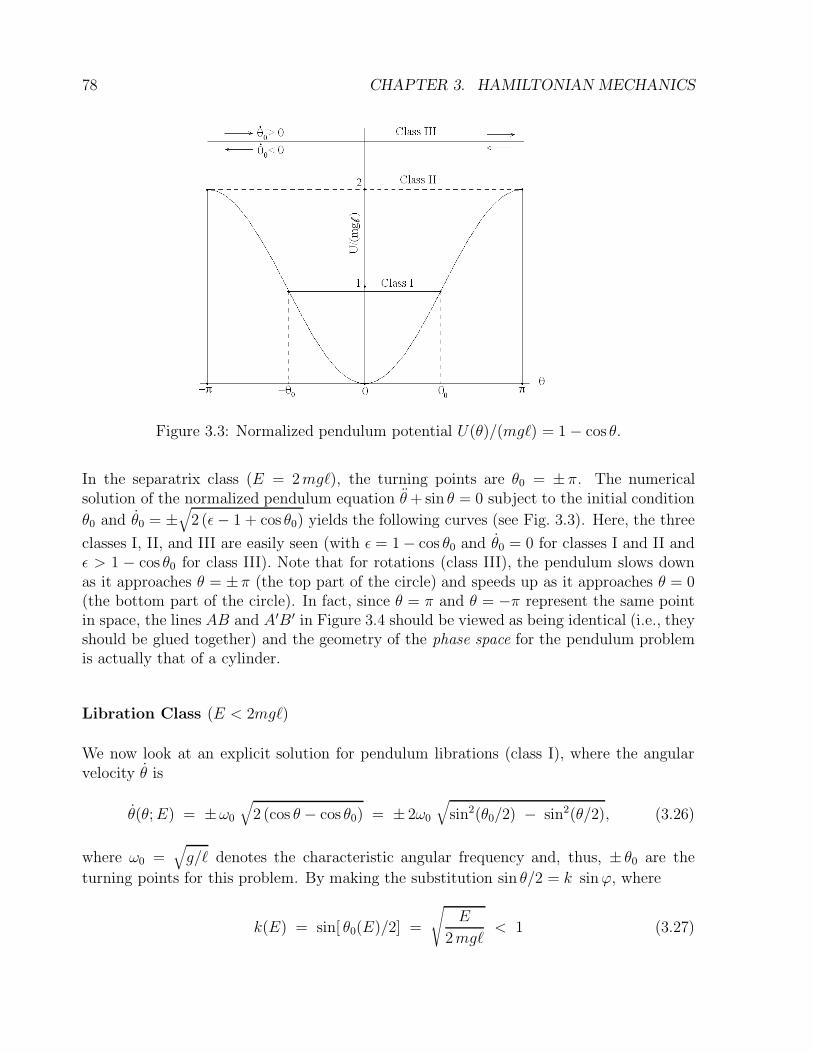
78 CHAPTER 3. HAMILTONIAN MECHANICS
Figure 3.3: Normalized pendulum potential U(θ)/(mg`) = 1 − cos θ.
In the separatrix class (E = 2mg`), the turning points are θ0 = ±π. The numericalsolution of the normalized pendulum equation θ+ sin θ = 0 subject to the initial condition
θ0 and θ0 = ±√
2 (ε− 1 + cos θ0) yields the following curves (see Fig. 3.3). Here, the three
classes I, II, and III are easily seen (with ε = 1 − cos θ0 and θ0 = 0 for classes I and II andε > 1 − cos θ0 for class III). Note that for rotations (class III), the pendulum slows downas it approaches θ = ±π (the top part of the circle) and speeds up as it approaches θ = 0(the bottom part of the circle). In fact, since θ = π and θ = −π represent the same pointin space, the lines AB and A′B ′ in Figure 3.4 should be viewed as being identical (i.e., theyshould be glued together) and the geometry of the phase space for the pendulum problemis actually that of a cylinder.
Libration Class (E < 2mg`)
We now look at an explicit solution for pendulum librations (class I), where the angularvelocity θ is
θ(θ;E) = ±ω0
√2 (cos θ − cos θ0) = ± 2ω0
√sin2(θ0/2) − sin2(θ/2), (3.26)
where ω0 =√g/` denotes the characteristic angular frequency and, thus, ± θ0 are the
turning points for this problem. By making the substitution sin θ/2 = k sinϕ, where
k(E) = sin[ θ0(E)/2] =
√E
2mg`< 1 (3.27)

3.5. ONE-DEGREE-OF-FREEDOM HAMILTONIAN DYNAMICS 79
Figure 3.4: Phase space of the pendulum
and ϕ = ±π/2 when θ = ± θ0, the libration solution of the pendulum problem is thus
ω0 t(θ;E) =∫ π/2
Θ(θ;E)
dϕ√
1 − k2 sin2 ϕ, (3.28)
where Θ(θ;E) = arcsin(k−1 sin θ/2). The inversion of this relation yields θ(t;E) expressedin terms of Jacobi elliptic functions (see Appendix A.3.2 for more details), while the periodof oscillation is defined as
ω0 T (E) = 4∫ π/2
0
dϕ√
1 − k2 sin2 ϕ= 4
∫ π/2
0dϕ
(
1 +k2
2sin2 ϕ + · · ·
)
,
= 2π
(
1 +k2
4+ · · ·
)
= 4 K(k), (3.29)
where K(k) denotes the complete elliptic integral of the first kind (see Figure 3.5 andAppendix A.3.2).
We note here that if k 1 (or θ0 1) the libration period of a pendulum is nearlyindependent of energy, T ' 2π/ω0. However, we also note that as E → 2mg` (k → 1 orθ0 → π), the libration period of the pendulum becomes infinitely large, i.e., T → ∞ inEq. (3.29) (see Figure 3.5).
Separatrix Class (E = 2mg`)
In the separatrix case (θ0 = π), the pendulum equation (3.26) yields the separatrix equa-tion ϕ = ω0 cosϕ, where ϕ = θ/2. The separatrix solution is expressed in terms of the
80 CHAPTER 3. HAMILTONIAN MECHANICS
Figure 3.5: Normalized pendulum period ω0 T (E)/2π as a function of the normalized energyk2 = E/(2mg`) for Libration Class I (k2 < 1) and Rotation Class III (k2 > 1); note that,for the Separatrix Class II (k2 = 1), the period is infinite.
transcendental equation
secϕ(t) = cosh(ω0t+ γ), (3.30)
where cosh γ = secϕ0 represents the initial condition. We again note that ϕ → π/2 (orθ → π) only as t→ ∞. Separatrices are associated with turning points s0 where U ′(s0) = 0and U ′′(s0) < 0, which are quite common in periodic dynamical systems as will be shownin Secs. 3.6 and 7.2.3.
Rotation Class (E > 2mg`)
The solution for rotations (class III) associated with the initial conditions θ0 = ±π and
1
2θ20 = ω2
0
(E
mg`− 2
)
=1
2θ2 − ω2
0
(1 + cos θ
),
or
θ = ±√θ20 + 2ω2
0 (1 + cos θ),
which shows that θ does not vanish for rotations. We now write cos θ = 1 − 2 sin2(θ/2)and define Ω2
0 = θ20 + 4ω2
0 , with so that
θ = ±Ω0
√1 − k−2 sin2(θ/2),
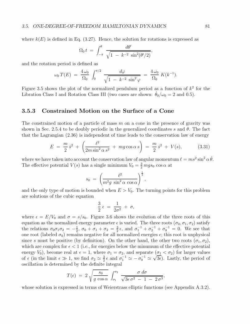
3.5. ONE-DEGREE-OF-FREEDOM HAMILTONIAN DYNAMICS 81
where k(E) is defined in Eq. (3.27). Hence, the solution for rotations is expressed as
Ω0 t =∫ θ
−π
dθ′√
1 − k−2 sin2(θ′/2),
and the rotation period is defined as
ω0 T (E) =4ω0
Ω0
∫ π/2
0
dϕ√
1 − k−2 sin2 ϕ=
4ω0
Ω0K(k−1).
Figure 3.5 shows the plot of the normalized pendulum period as a function of k2 for theLibration Class I and Rotation Class III (two cases are shown: θ0/ω0 = 2 and 0.5).
3.5.3 Constrained Motion on the Surface of a Cone
The constrained motion of a particle of mass m on a cone in the presence of gravity wasshown in Sec. 2.5.4 to be doubly periodic in the generalized coordinates s and θ. The factthat the Lagrangian (2.36) is independent of time leads to the conservation law of energy
E =m
2s2 +
(`2
2m sin2 α s2+ mg cosα s
)
=m
2s2 + V (s), (3.31)
where we have taken into account the conservation law of angular momentum ` = ms2 sin2 α θ.The effective potential V (s) has a single minimum V0 = 3
2mgs0 cosα at
s0 =
(`2
m2g sin2 α cosα
) 1
3
,
and the only type of motion is bounded when E > V0. The turning points for this problemare solutions of the cubic equation
3
2ε =
1
2σ2+ σ,
where ε = E/V0 and σ = s/s0. Figure 3.6 shows the evolution of the three roots of thisequation as the normalized energy parameter ε is varied. The three roots (σ0, σ1, σ2) satisfythe relations σ0σ1σ2 = −1
2, σ0 + σ1 + σ2 = 3
2ε, and σ−1
1 + σ−12 + σ−1
0 = 0. We see thatone root (labeled σ0) remains negative for all normalized energies ε; this root is unphysicalsince s must be positive (by definition). On the other hand, the other two roots (σ1, σ2),which are complex for ε < 1 (i.e., for energies below the minumum of the effective potentialenergy V0), become real at ε = 1, where σ1 = σ2, and separate (σ1 < σ2) for larger valuesof ε (in the limit ε 1, we find σ2 ' 3
2ε and σ−1
1 ' −σ−10 '
√3ε). Lastly, the period of
oscillation is determined by the definite integral
T (ε) = 2
√s0
g cosα
∫ σ2
σ1
σ dσ√3ε σ2 − 1 − 2σ3
,
whose solution is expressed in terms of Weierstrass elliptic functions (see Appendix A.3.2).
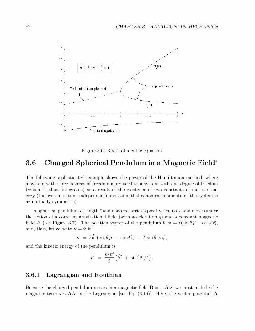
82 CHAPTER 3. HAMILTONIAN MECHANICS
Figure 3.6: Roots of a cubic equation
3.6 Charged Spherical Pendulum in a Magnetic Field∗
The following sophisticated example shows the power of the Hamiltonian method, wherea system with three degrees of freedom is reduced to a system with one degree of freedom(which is, thus, integrable) as a result of the existence of two constants of motion: en-ergy (the system is time independent) and azimuthal canonical momentum (the system isazimuthally symmetric).
A spherical pendulum of length ` and massm carries a positive charge e and moves underthe action of a constant gravitational field (with acceleration g) and a constant magneticfield B (see Figure 3.7). The position vector of the pendulum is x = `(sin θ ρ − cos θ z),and, thus, its velocity v = x is
v = ` θ (cos θ ρ + sin θ z) + ` sin θ ϕ ϕ,
and the kinetic energy of the pendulum is
K =m`2
2
(θ2 + sin2 θ ϕ2
).
3.6.1 Lagrangian and Routhian
Because the charged pendulum moves in a magnetic field B = −B z, we must include themagnetic term v · eA/c in the Lagrangian [see Eq. (3.16)]. Here, the vector potential A
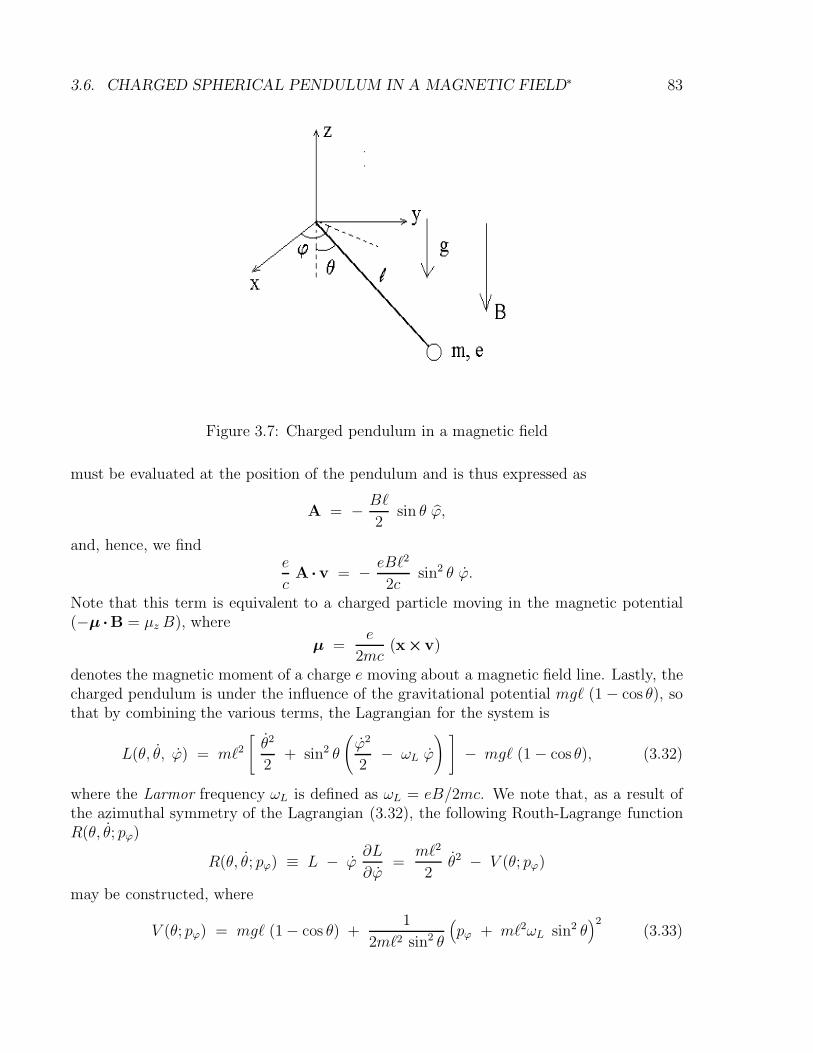
3.6. CHARGED SPHERICAL PENDULUM IN A MAGNETIC FIELD∗ 83
Figure 3.7: Charged pendulum in a magnetic field
must be evaluated at the position of the pendulum and is thus expressed as
A = − B`
2sin θ ϕ,
and, hence, we finde
cA · v = − eB`2
2csin2 θ ϕ.
Note that this term is equivalent to a charged particle moving in the magnetic potential(−µ ·B = µz B), where
µ =e
2mc(x×v)
denotes the magnetic moment of a charge e moving about a magnetic field line. Lastly, thecharged pendulum is under the influence of the gravitational potential mg` (1 − cos θ), sothat by combining the various terms, the Lagrangian for the system is
L(θ, θ, ϕ) = m`2[θ2
2+ sin2 θ
(ϕ2
2− ωL ϕ
) ]
− mg` (1 − cos θ), (3.32)
where the Larmor frequency ωL is defined as ωL = eB/2mc. We note that, as a result ofthe azimuthal symmetry of the Lagrangian (3.32), the following Routh-Lagrange functionR(θ, θ; pϕ)
R(θ, θ; pϕ) ≡ L − ϕ∂L
∂ϕ=
m`2
2θ2 − V (θ; pϕ)
may be constructed, where
V (θ; pϕ) = mg` (1 − cos θ) +1
2m`2 sin2 θ
(pϕ + m`2ωL sin2 θ
)2(3.33)
84 CHAPTER 3. HAMILTONIAN MECHANICS
represents an effective potential under which the charged spherical pendulum moves.
3.6.2 Routh-Euler-Lagrange equations
The Routh-Euler-Lagrange equation for θ is expressed in terms of the effective potential(3.33) as
d
dt
(∂R
∂θ
)
=∂R
∂θ→ m`2 θ = − ∂V
∂θ,
which yields
θ +g
`sin θ = sin θ cos θ
[ (pϕ
m`2 sin2 θ
)2
− ω2L
]
. (3.34)
Not surprisingly the integration of this second-order differential equation for θ is complex(see below). It turns out, however, that the Hamiltonian formalism gives us glimpses intothe gobal structure of general solutions of this equation.
3.6.3 Hamiltonian
The Hamiltonian for the charged pendulum in a magnetic field is obtained through theLegendre transformation (3.4):
H = θ∂L
∂θ+ ϕ
∂L
∂ϕ− L
=p2θ
2m`2+
1
2m`2 sin2 θ
(pϕ + m`2ωL sin2 θ
)2+ mg` (1 − cos θ). (3.35)
The Hamilton’s equations for (θ, pθ) are
θ =∂H
∂pθ=
pθm`2
pθ = − ∂H
∂θ= − mg` sin θ + m`2 sin θ cos θ
[ (pϕ
m`2 sin2 θ
)2
− ω2L
]
,
while the Hamilton’s equations for (ϕ, pϕ) are
ϕ =∂H
∂pϕ=
pϕm`2 sin2 θ
+ ωL
pϕ = − ∂H
∂ϕ= 0.
It is readily seen that these Hamilton equations lead to the same equations as the Euler-Lagrange equations for θ and ϕ.
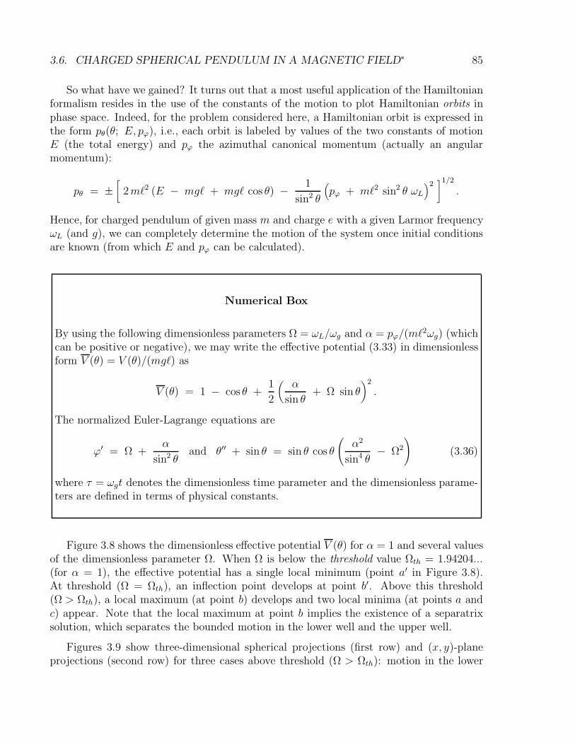
3.6. CHARGED SPHERICAL PENDULUM IN A MAGNETIC FIELD∗ 85
So what have we gained? It turns out that a most useful application of the Hamiltonianformalism resides in the use of the constants of the motion to plot Hamiltonian orbits inphase space. Indeed, for the problem considered here, a Hamiltonian orbit is expressed inthe form pθ(θ; E, pϕ), i.e., each orbit is labeled by values of the two constants of motionE (the total energy) and pϕ the azimuthal canonical momentum (actually an angularmomentum):
pθ = ±[
2m`2 (E − mg` + mg` cos θ) − 1
sin2 θ
(pϕ + m`2 sin2 θ ωL
)2]1/2
.
Hence, for charged pendulum of given mass m and charge e with a given Larmor frequencyωL (and g), we can completely determine the motion of the system once initial conditionsare known (from which E and pϕ can be calculated).
Numerical Box
By using the following dimensionless parameters Ω = ωL/ωg and α = pϕ/(m`2ωg) (which
can be positive or negative), we may write the effective potential (3.33) in dimensionlessform V (θ) = V (θ)/(mg`) as
V (θ) = 1 − cos θ +1
2
(α
sin θ+ Ω sin θ
)2
.
The normalized Euler-Lagrange equations are
ϕ′ = Ω +α
sin2 θand θ′′ + sin θ = sin θ cos θ
(α2
sin4 θ− Ω2
)
(3.36)
where τ = ωgt denotes the dimensionless time parameter and the dimensionless parame-ters are defined in terms of physical constants.
Figure 3.8 shows the dimensionless effective potential V (θ) for α = 1 and several valuesof the dimensionless parameter Ω. When Ω is below the threshold value Ωth = 1.94204...(for α = 1), the effective potential has a single local minimum (point a′ in Figure 3.8).At threshold (Ω = Ωth), an inflection point develops at point b′. Above this threshold(Ω > Ωth), a local maximum (at point b) develops and two local minima (at points a andc) appear. Note that the local maximum at point b implies the existence of a separatrixsolution, which separates the bounded motion in the lower well and the upper well.
Figures 3.9 show three-dimensional spherical projections (first row) and (x, y)-planeprojections (second row) for three cases above threshold (Ω > Ωth): motion in the lower
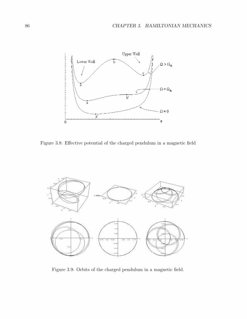
86 CHAPTER 3. HAMILTONIAN MECHANICS
Figure 3.8: Effective potential of the charged pendulum in a magnetic field
Figure 3.9: Orbits of the charged pendulum in a magnetic field.
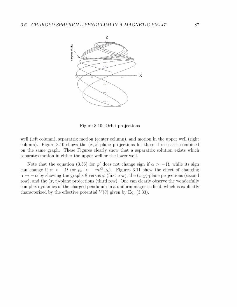
3.6. CHARGED SPHERICAL PENDULUM IN A MAGNETIC FIELD∗ 87
Figure 3.10: Orbit projections
well (left column), separatrix motion (center column), and motion in the upper well (rightcolumn). Figure 3.10 shows the (x, z)-plane projections for these three cases combinedon the same graph. These Figures clearly show that a separatrix solution exists whichseparates motion in either the upper well or the lower well.
Note that the equation (3.36) for ϕ′ does not change sign if α > −Ω, while its signcan change if α < −Ω (or pϕ < −m`2 ωL). Figures 3.11 show the effect of changingα→ −α by showing the graphs θ versus ϕ (first row), the (x, y)-plane projections (secondrow), and the (x, z)-plane projections (third row). One can clearly observe the wonderfullycomplex dynamics of the charged pendulum in a uniform magnetic field, which is explicitlycharacterized by the effective potential V (θ) given by Eq. (3.33).
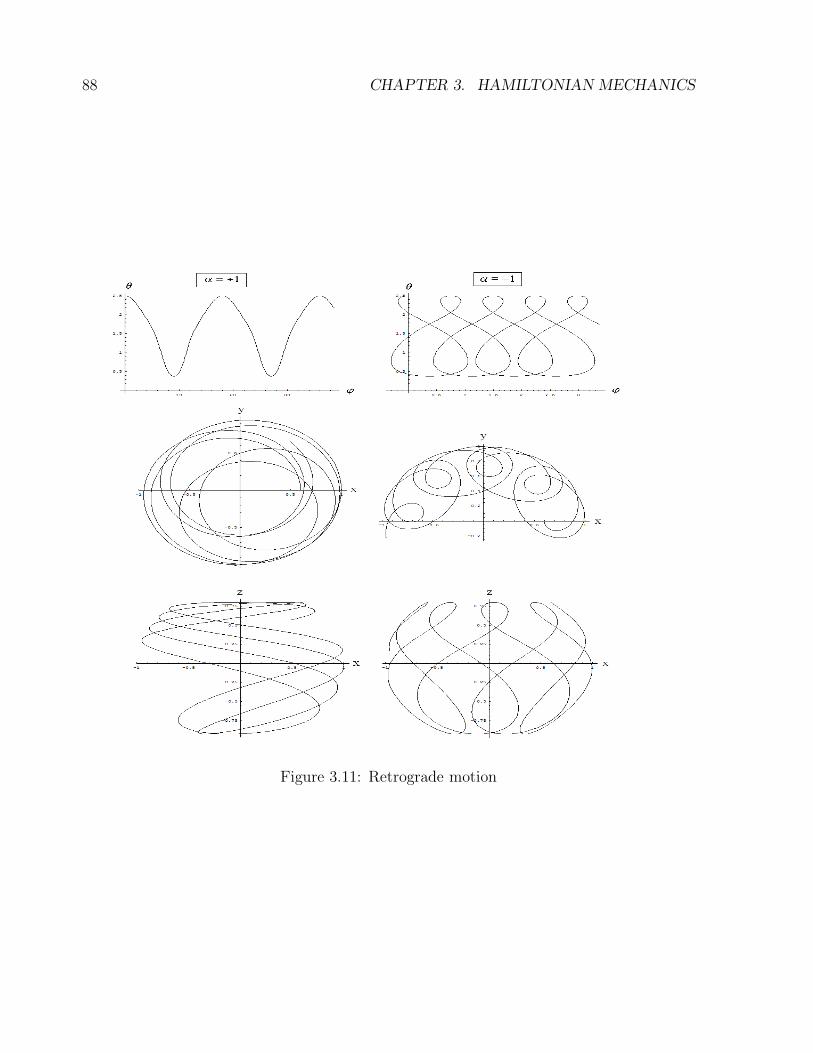
88 CHAPTER 3. HAMILTONIAN MECHANICS
Figure 3.11: Retrograde motion
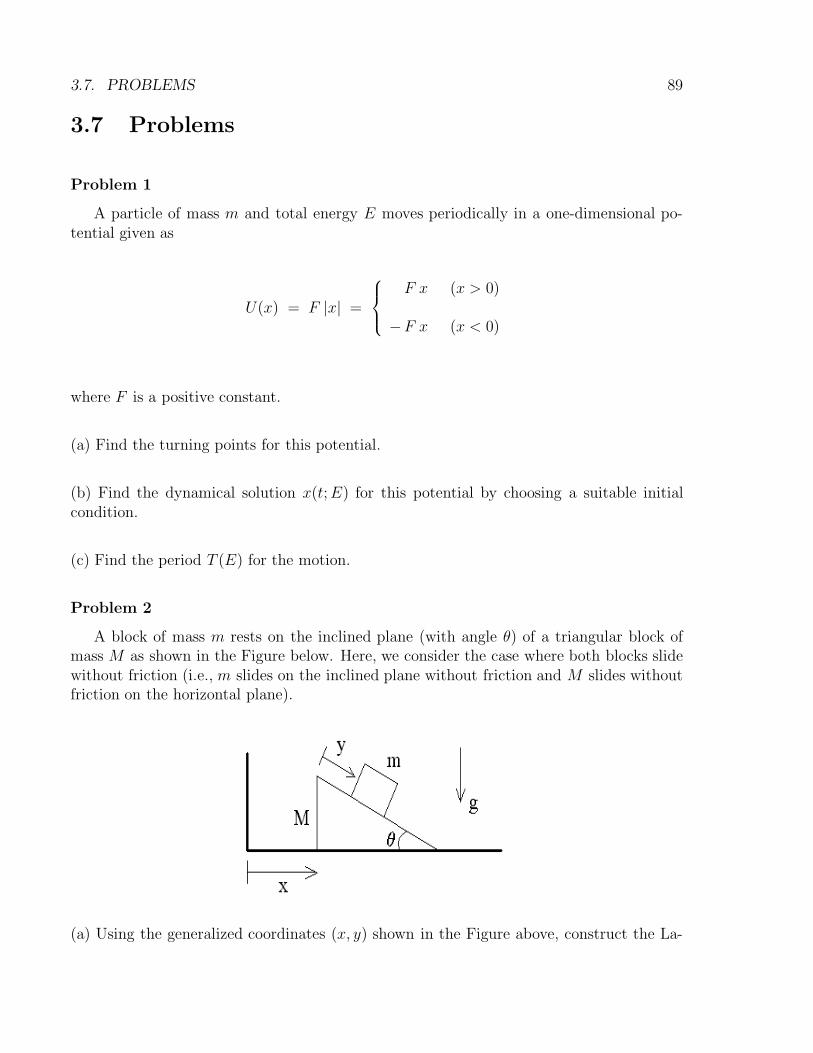
3.7. PROBLEMS 89
3.7 Problems
Problem 1
A particle of mass m and total energy E moves periodically in a one-dimensional po-tential given as
U(x) = F |x| =
F x (x > 0)
−F x (x < 0)
where F is a positive constant.
(a) Find the turning points for this potential.
(b) Find the dynamical solution x(t;E) for this potential by choosing a suitable initialcondition.
(c) Find the period T (E) for the motion.
Problem 2
A block of mass m rests on the inclined plane (with angle θ) of a triangular block ofmass M as shown in the Figure below. Here, we consider the case where both blocks slidewithout friction (i.e., m slides on the inclined plane without friction and M slides withoutfriction on the horizontal plane).
(a) Using the generalized coordinates (x, y) shown in the Figure above, construct the La-
90 CHAPTER 3. HAMILTONIAN MECHANICS
grangian L(x, x, y, y).
(b) Derive the Euler-Lagrange equations for x and y.
(c) Calculate the canonical momenta
px(x, x, y, y) =∂L
∂xand py(x, x, y, y) =
∂L
∂y,
and invert these expressions to find the functions x(x, px, y, py) and y(x, px, y, py).
(d) Calculate the Hamiltonian H(x, px, y, py) for this system by using the Legendre trans-formation
H(x, px, y, py) = px x + py y − L(x, x, y, y),
where the functions x(x, px, y, py) and y(x, px, y, py) are used.
(e) Find which of the two momenta found in Part (c) is a constant of the motion anddiscuss why it is so. If the two blocks start from rest, what is the value of this constant ofmotion?
Problem 3
Consider all possible orbits of a unit-mass particle moving in the dimensionless potentialU(x) = 1−x2/2 + x4/16. Here, orbits are solutions of the equation of motion x = −U ′(x)and the dimensionless energy equation is E = x2/2 + U(x).
(a) Draw the potential U(x) and identify all possible unbounded and bounded orbits (withtheir respective energy ranges).
(b) For each orbit found in part (a), find the turning point(s) for each energy level.
(c) Sketch the phase portrait (x, x) showing all orbits (including the separatrix orbit).
(d) Show that the separatrix orbit (with initial conditions x0 =√
8 and x0 = 0) is expressedas x(t) =
√8 sech(t) by solving the integral
t(x) =∫ √
8
x
ds√s2 (1 − s2/8)
.
(Hint: use the hyperbolic trigonometric substitution s =√
8 sech ξ.)
(e) Write a numerical code to solve the second-order ordinary differential equation x =x−x3/4 by choosing appropriate initial conditions needed to obtain all the possible orbits.
3.7. PROBLEMS 91
Problem 4
When a particle (of mass m) moving under the potential U(x) is perturbed by thepotential δU(x), its period (3.24) is changed by a small amount defined as
δT = −√
2m∂
∂E
∫ x2
x1
δU(x) dx√E − U(x)
,
where x1,2 are the turning points of the unperturbed problem. Calculate the change inthe period of a particle moving in the quadratic potential U(x) = mω2 x2/2 introduced bythe perturbation potential δU(x) = ε x4. Here, ω denotes the unperturbed frequency, theparticle is trapped in the region −a ≤ x ≤ a, and ε is a constant that satisfies the conditionε mω2/(2a2).

92 CHAPTER 3. HAMILTONIAN MECHANICS
Chapter 4
Motion in a Central-Force Field
4.1 Motion in a Central-Force Field
A particle moves under the influence of a central-force field F(r) = F (r) r(θ, ϕ) if the forceon the particle is independent of the angular position (θ, ϕ) of the particle about the centerof force and depends only on its distance r from the center of force. Here, the magnitudeF (r) (which is positive for a repulsive force and negative for an attractive force) is definedin terms of the central potential U(r) as F (r) = −U ′(r). Note that, for a central-forcepotential U(r), the angular momentum L = ` z in the CM frame is a constant of the motionsince r×∇U(r) = 0.
4.1.1 Lagrangian Formalism
The motion of two particles in an isolated system takes place on a two-dimensional plane,which we, henceforth, take to be the (x, y)-plane and, hence, the constant angular mo-mentum is L = ` z. When these particles move in a central-force field, the center-of-massLagrangian is simply
L =µ
2
(r2 + r2 θ2
)− U(r), (4.1)
where µ denotes the reduced mass for the two-particle system and polar coordinates (r, θ)are most conveniently used, with x = r cos θ and y = r sin θ. Since the potential U isindependent of θ, the canonical angular momentum
pθ =∂L
∂θ= µr2 θ ≡ ` (4.2)
93
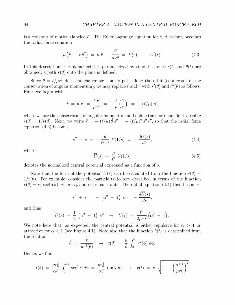
94 CHAPTER 4. MOTION IN A CENTRAL-FORCE FIELD
is a constant of motion (labeled `). The Euler-Lagrange equation for r, therefore, becomesthe radial force equation
µ(r − r θ2
)= µ r − `2
µr3= F (r) ≡ −U ′(r). (4.3)
In this description, the planar orbit is parametrized by time, i.e., once r(t) and θ(t) areobtained, a path r(θ) onto the plane is defined.
Since θ = `/µr2 does not change sign on its path along the orbit (as a result of theconservation of angular momentum), we may replace r and r with r′(θ) and r′′(θ) as follows.First, we begin with
r = θ r′ =` r′
µr2= − `
µ
(1
r
)′= − (`/µ) s′,
where we use the conservation of angular momentum and define the new dependent variables(θ) = 1/r(θ). Next, we write r = − (`/µ) θ s′′ = − (`/µ)2 s2 s′′, so that the radial forceequation (4.3) becomes
s′′ + s = − µ
`2 s2F (1/s) ≡ − dU (s)
ds, (4.4)
whereU(s) =
µ
`2U(1/s) (4.5)
denotes the normalized central potential expressed as a function of s.
Note that the form of the potential U(r) can be calculated from the function s(θ) =1/r(θ). For example, consider the particle trajectory described in terms of the functionr(θ) = r0 sec(α θ), where r0 and α are constants. The radial equation (4.4) then becomes
s′′ + s = −(α2 − 1
)s = − dU(s)
ds,
and thus
U(s) =1
2
(α2 − 1
)s2 → U(r) =
`2
2µr2
(α2 − 1
).
We note here that, as expected, the central potential is either repulsive for α > 1 orattractive for α < 1 (see Figure 4.1). Note also that the function θ(t) is determined fromthe relation
θ =`
µr2(θ)→ t(θ) =
µ
`
∫ θ
0r2(φ) dφ.
Hence, we find
t(θ) =µr2
0
α`
∫ αθ
0sec2 φ dφ =
µr20
α`tan(αθ) → r(t) = r0
√√√√1 +
(α` t
µr20
)2
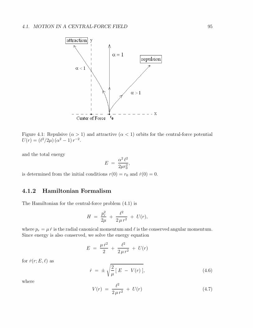
4.1. MOTION IN A CENTRAL-FORCE FIELD 95
Figure 4.1: Repulsive (α > 1) and attractive (α < 1) orbits for the central-force potentialU(r) = (`2/2µ) (α2 − 1) r−2.
and the total energy
E =α2 `2
2µr20
,
is determined from the initial conditions r(0) = r0 and r(0) = 0.
4.1.2 Hamiltonian Formalism
The Hamiltonian for the central-force problem (4.1) is
H =p2r
2µ+
`2
2µr2+ U(r),
where pr = µ r is the radial canonical momentum and ` is the conserved angular momentum.Since energy is also conserved, we solve the energy equation
E =µ r2
2+
`2
2µr2+ U(r)
for r(r;E, `) as
r = ±√
2
µ[ E − V (r) ], (4.6)
where
V (r) =`2
2µr2+ U(r) (4.7)
96 CHAPTER 4. MOTION IN A CENTRAL-FORCE FIELD
is the effective potential for central-force problems and the sign ± in Eq. (4.6) depends oninitial conditions. Hence, Eq. (4.6) yields the integral solution
t(r;E, `) = ±∫
dr√
(2/µ) [E − V (r)]. (4.8)
We can also the energy equation
µE/`2 =s′2
2+
s2
2+ U(s), (4.9)
to obtains′(θ) = ±
√ε− 2U (s) − s2, (4.10)
where the normalized energy ε is defined as
ε =2µE
`2. (4.11)
Hence, for a given central-force potential U(r), we can solve for r(θ) = 1/s(θ) by integrating
θ(s) = −∫ s
s0
dσ√ε− 2U (σ) − σ2
, (4.12)
where s0 defines θ(s0) = 0, and performing the inversion θ(s) → s(θ) = 1/r(θ).
4.1.3 Turning Points
Eq. (4.10) yields the following energy equation
E =µ
2r2 +
`2
2µr2+ U(r) =
`2
2µ
[(s′)2 + s2 + 2U (s)
],
where s′ = −µr/`. Turning points are those special values of rn (or sn) (n = 1, 2, ...) forwhich
E = U(rn) +`2
2µr2n
=`2
µ
[
U(sn) +s2n
2
]
,
i.e., r (or s′) vanishes at these points. If two non-vanishing turning points r2 < r1 < ∞(or 0 < s1 < s2) exist, the motion is said to be bounded in the interval r2 < r < r1 (ors1 < s < s2), otherwise the motion is unbounded. If the motion is bounded, the angularperiod ∆θ is defined as
∆θ(s) = 2∫ s2
s1
ds√ε− 2U (s) − s2
. (4.13)
Here, the bounded orbit is closed only if ∆θ is a rational multiple of 2π.
4.2. HOMOGENEOUS CENTRAL POTENTIALS∗ 97
4.2 Homogeneous Central Potentials∗
An important class of central potentials is provided by homogeneous potentials that satisfythe condition U(λ r) = λn U(r), where λ denotes a rescaling parameter and n denotes theorder of the homogeneous potential.
4.2.1 The Virial Theorem
The Virial Theorem is an important theorem in Celestial Mechanics and Astrophysics. Webegin with the time derivative of the quantity S =
∑i pi · ri:
dS
dt=
∑
i
(dpidt
· ri + pi ·dridt
)
, (4.14)
where the summation is over all particles in a mechanical system under the influence of aself-interaction potential
U =1
2
∑
i, j 6=iU(ri − rj).
We note, however, that since Q itself can be written as a time derivative
S =∑
i
midridt
· ri =d
dt
(1
2
∑
i
mi |ri|2)
=1
2
dIdt,
where I denotes the moment of inertia of the system and that, using Hamilton’s equations
dridt
=pi
miand
dpidt
= −∑
j 6=i∇i U(ri − rj),
Eq. (4.14) can also be written as
1
2
d2Idt2
=∑
i
|pi|2mi
− ri ·∑
j 6=i∇iUij
= 2 K −∑
i, j 6=iri ·∇iUij, (4.15)
where K denotes the kinetic energy of the mechanical system. Next, using Newton’s ThirdLaw, we write
∑
i, j 6=iri ·∇iUij =
1
2
∑
i, j 6=i(ri − rj) ·∇U(ri − rj),
and, for a homogeneous central potential of order n, we find r ·∇U(r) = n U(r), so that
1
2
∑
i, j 6=i(ri − rj) ·∇U(ri − rj) = n U.
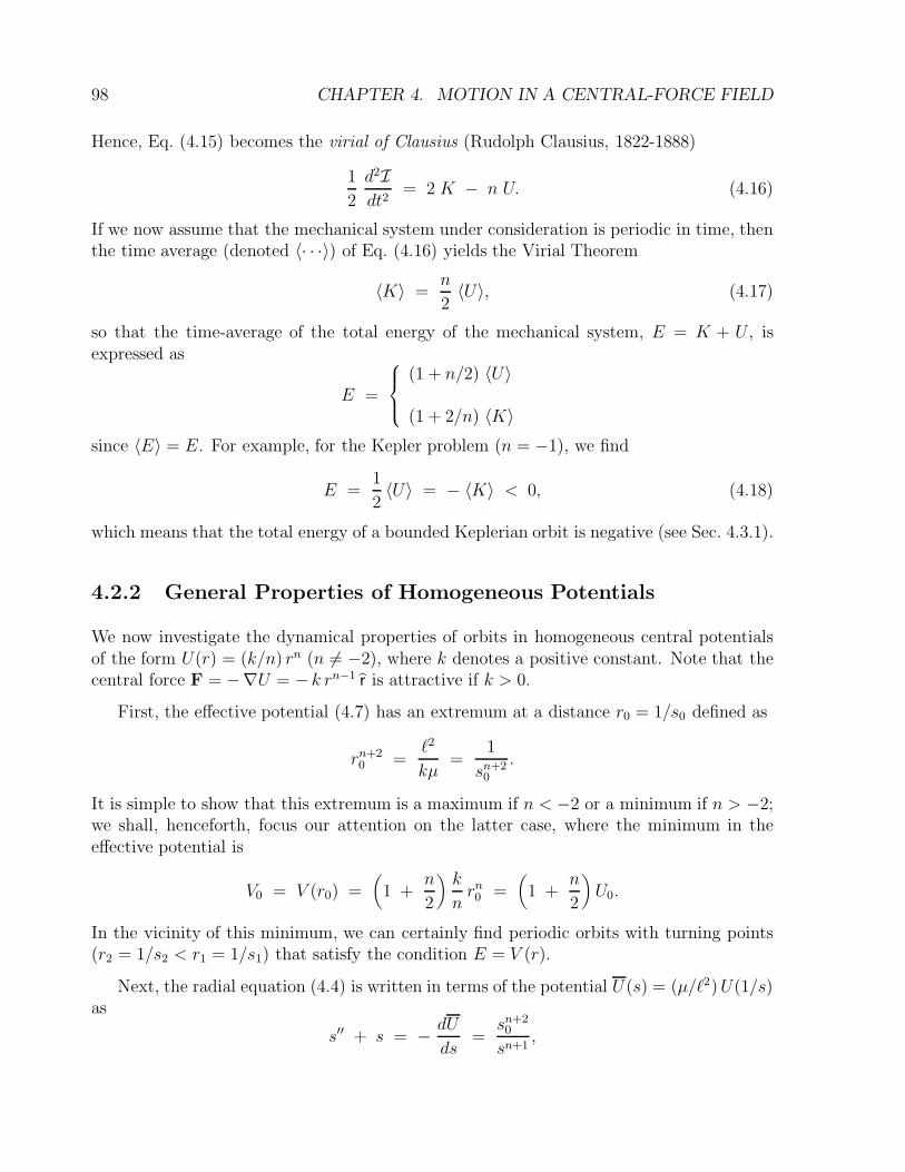
98 CHAPTER 4. MOTION IN A CENTRAL-FORCE FIELD
Hence, Eq. (4.15) becomes the virial of Clausius (Rudolph Clausius, 1822-1888)
1
2
d2Idt2
= 2 K − n U. (4.16)
If we now assume that the mechanical system under consideration is periodic in time, thenthe time average (denoted 〈· · ·〉) of Eq. (4.16) yields the Virial Theorem
〈K〉 =n
2〈U〉, (4.17)
so that the time-average of the total energy of the mechanical system, E = K + U , isexpressed as
E =
(1 + n/2) 〈U〉
(1 + 2/n) 〈K〉since 〈E〉 = E. For example, for the Kepler problem (n = −1), we find
E =1
2〈U〉 = − 〈K〉 < 0, (4.18)
which means that the total energy of a bounded Keplerian orbit is negative (see Sec. 4.3.1).
4.2.2 General Properties of Homogeneous Potentials
We now investigate the dynamical properties of orbits in homogeneous central potentialsof the form U(r) = (k/n) rn (n 6= −2), where k denotes a positive constant. Note that thecentral force F = −∇U = − k rn−1 r is attractive if k > 0.
First, the effective potential (4.7) has an extremum at a distance r0 = 1/s0 defined as
rn+20 =
`2
kµ=
1
sn+20
.
It is simple to show that this extremum is a maximum if n < −2 or a minimum if n > −2;we shall, henceforth, focus our attention on the latter case, where the minimum in theeffective potential is
V0 = V (r0) =(1 +
n
2
)k
nrn0 =
(1 +
n
2
)U0.
In the vicinity of this minimum, we can certainly find periodic orbits with turning points(r2 = 1/s2 < r1 = 1/s1) that satisfy the condition E = V (r).
Next, the radial equation (4.4) is written in terms of the potential U (s) = (µ/`2)U(1/s)as
s′′ + s = − dU
ds=
sn+20
sn+1,
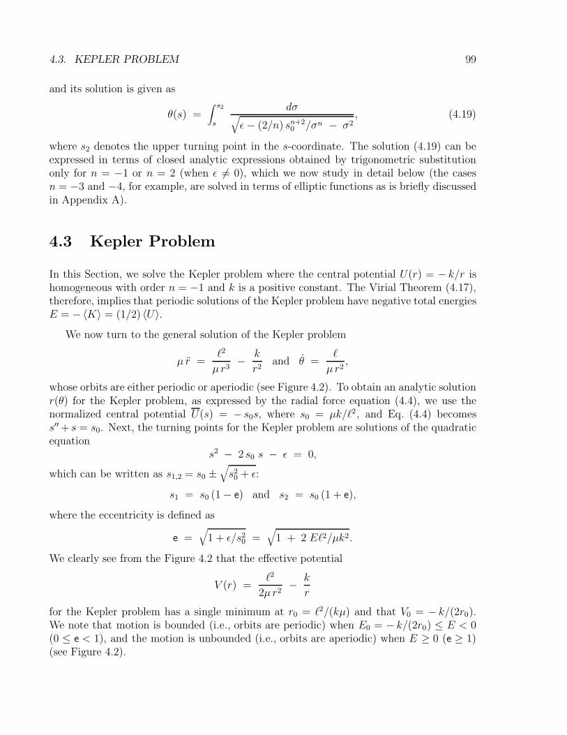
4.3. KEPLER PROBLEM 99
and its solution is given as
θ(s) =∫ s2
s
dσ√ε− (2/n) sn+2
0 /σn − σ2, (4.19)
where s2 denotes the upper turning point in the s-coordinate. The solution (4.19) can beexpressed in terms of closed analytic expressions obtained by trigonometric substitutiononly for n = −1 or n = 2 (when ε 6= 0), which we now study in detail below (the casesn = −3 and −4, for example, are solved in terms of elliptic functions as is briefly discussedin Appendix A).
4.3 Kepler Problem
In this Section, we solve the Kepler problem where the central potential U(r) = − k/r ishomogeneous with order n = −1 and k is a positive constant. The Virial Theorem (4.17),therefore, implies that periodic solutions of the Kepler problem have negative total energiesE = −〈K〉 = (1/2) 〈U〉.
We now turn to the general solution of the Kepler problem
µ r =`2
µr3− k
r2and θ =
`
µ r2,
whose orbits are either periodic or aperiodic (see Figure 4.2). To obtain an analytic solutionr(θ) for the Kepler problem, as expressed by the radial force equation (4.4), we use thenormalized central potential U(s) = − s0s, where s0 = µk/`2, and Eq. (4.4) becomess′′ + s = s0. Next, the turning points for the Kepler problem are solutions of the quadraticequation
s2 − 2 s0 s − ε = 0,
which can be written as s1,2 = s0 ±√s20 + ε:
s1 = s0 (1 − e) and s2 = s0 (1 + e),
where the eccentricity is defined as
e =√
1 + ε/s20 =
√1 + 2 E`2/µk2.
We clearly see from the Figure 4.2 that the effective potential
V (r) =`2
2µr2− k
r
for the Kepler problem has a single minimum at r0 = `2/(kµ) and that V0 = − k/(2r0).We note that motion is bounded (i.e., orbits are periodic) when E0 = − k/(2r0) ≤ E < 0(0 ≤ e < 1), and the motion is unbounded (i.e., orbits are aperiodic) when E ≥ 0 (e ≥ 1)(see Figure 4.2).
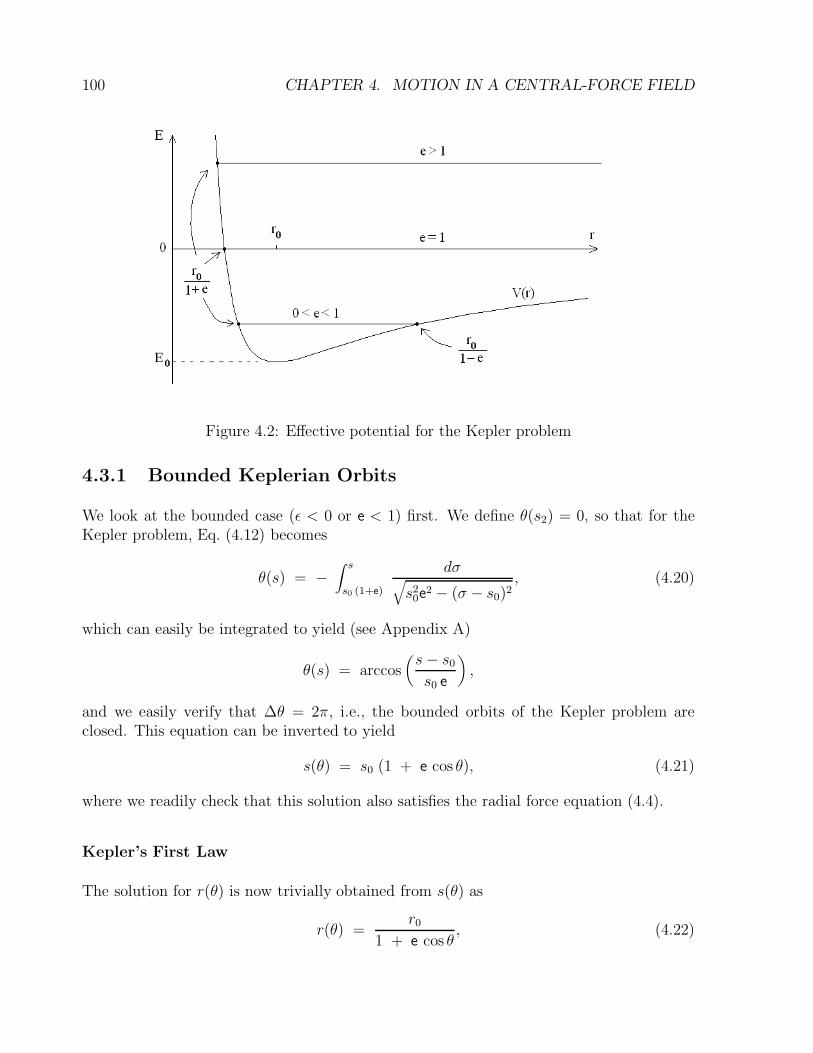
100 CHAPTER 4. MOTION IN A CENTRAL-FORCE FIELD
Figure 4.2: Effective potential for the Kepler problem
4.3.1 Bounded Keplerian Orbits
We look at the bounded case (ε < 0 or e < 1) first. We define θ(s2) = 0, so that for theKepler problem, Eq. (4.12) becomes
θ(s) = −∫ s
s0 (1+e)
dσ√s20e
2 − (σ − s0)2, (4.20)
which can easily be integrated to yield (see Appendix A)
θ(s) = arccos(s− s0
s0 e
),
and we easily verify that ∆θ = 2π, i.e., the bounded orbits of the Kepler problem areclosed. This equation can be inverted to yield
s(θ) = s0 (1 + e cos θ), (4.21)
where we readily check that this solution also satisfies the radial force equation (4.4).
Kepler’s First Law
The solution for r(θ) is now trivially obtained from s(θ) as
r(θ) =r0
1 + e cos θ, (4.22)
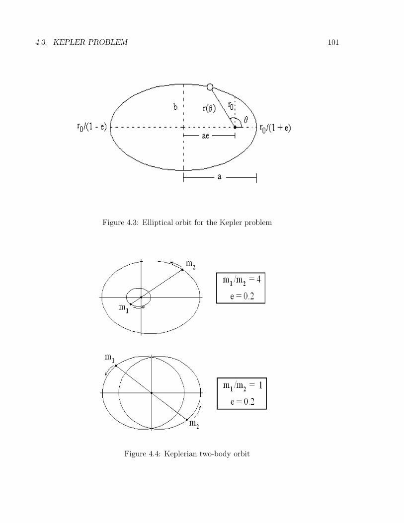
4.3. KEPLER PROBLEM 101
Figure 4.3: Elliptical orbit for the Kepler problem
Figure 4.4: Keplerian two-body orbit
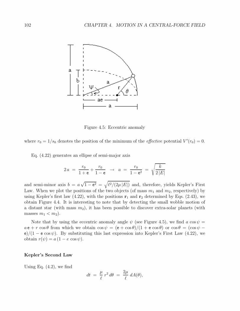
102 CHAPTER 4. MOTION IN A CENTRAL-FORCE FIELD
Figure 4.5: Eccentric anomaly
where r0 = 1/s0 denotes the position of the minimum of the effective potential V ′(r0) = 0.
Eq. (4.22) generates an ellipse of semi-major axis
2a =r0
1 + e+
r01 − e
→ a =r0
1 − e2=
√k
2 |E|
and semi-minor axis b = a√
1 − e2 =√`2/(2µ |E|) and, therefore, yields Kepler’s First
Law. When we plot the positions of the two objects (of mass m1 and m2, respectively) byusing Kepler’s first law (4.22), with the positions r1 and r2 determined by Eqs. (2.43), weobtain Figure 4.4. It is interesting to note that by detecting the small wobble motion ofa distant star (with mass m2), it has been possible to discover extra-solar planets (withmasses m1 < m2).
Note that by using the eccentric anomaly angle ψ (see Figure 4.5), we find a cosψ =a e + r cos θ from which we obtain cosψ = (e + cos θ)/(1 + e cos θ) or cos θ = (cosψ −e)/(1 − e cosψ). By substituting this last expression into Kepler’s First Law (4.22), weobtain r(ψ) = a (1 − e cosψ).
Kepler’s Second Law
Using Eq. (4.2), we find
dt =µ
`r2 dθ =
2µ
`dA(θ),
4.3. KEPLER PROBLEM 103
where dA(θ) = (∫r dr) dθ = 1
2[r(θ)]2 dθ denotes an infinitesimal area swept by dθ at radius
r(θ). When integrated, this relation yields Kepler’s Second law
∆t =2µ
`∆A, (4.23)
i.e., equal areas ∆A are swept in equal times ∆t since µ and ` are constants.
Kepler’s Third Law
The orbital period T of a bound system is defined as
T =∫ 2π
0
dθ
θ=
µ
`
∫ 2π
0r2 dθ =
2µ
`A =
2π µ
`a b
where A = π ab denotes the area of an ellipse with semi-major axis a and semi-minor axisb; here, we used the identity
∫ 2π
0
dθ
(1 + e cos θ)2=
2π
(1 − e2)3/2.
Using the expressions for a and b found above, we find
T =2π µ
`· k
2|E| ·√√√√ `2
2µ |E| = 2π
√√√√ µk2
(2 |E|)3.
If we now substitute the expression for a = k/2|E| and square both sides of this equation,we obtain Kepler’s Third Law
T 2 =(2π)2µ
ka3. (4.24)
In Newtonian gravitational theory, where k/µ = G (m1 + m2), we find that, althoughKepler’s Third Law states that T 2/a3 is a constant for all planets in the solar system,which is only an approximation that holds for m1 m2 (true for all solar planets).
4.3.2 Unbounded Keplerian Orbits
We now look at the case where the total energy is positive or zero (i.e., e ≥ 1). Eq. (4.22)yields r (1 + e cos θ) = r0 or the hyperbola equation
(√e2 − 1 x − e r0√
e2 − 1
)2
− y2 =r20
e2 − 1.
For e = 1, the particle orbit is a parabola x = (r20 − y2)/2r0, with distance of closest
approach at x(0) = r0/2.

104 CHAPTER 4. MOTION IN A CENTRAL-FORCE FIELD
Figure 4.6: Bounded and unbounded orbits for the Kepler problem
4.3.3 Laplace-Runge-Lenz Vector∗
Since the orientation of the unperturbed Keplerian ellipse is constant (i.e., it does notprecess), it turns out there exists a third constant of the motion for the Kepler problem(in addition to energy and angular momentum); we note, however, that only two of thesethree invariants are independent.
Let us now investigate this additional constant of the motion for the Kepler problem.First, we consider the time derivative of the vector p×L, where the linear momentum p
and angular momentum L are
p = µ(r r + rθ θ
)and L = ` z = µr2θ z.
The time derivative of the linear momentum is p = −∇U(r) = −U ′(r) r while the angularmomentum L = r×p is itself a constant of the motion so that
d
dt(p×L) =
dp
dt×L = − µ ∇U × (r× r)
= − µr ·∇U r + µr ·∇U r.
By re-arranging some terms (and using r ·∇U = dU/dt for time-independent potentials),we find
d
dt(p×L) = − d
dt(µU r) + µ (r ·∇U + U) r,
ordA
dt= µ (r ·∇U + U) r, (4.25)
4.3. KEPLER PROBLEM 105
where the Laplace-Runge-Lenz (LRL) vector is defined as
A = p× L + µU(r) r. (4.26)
We immediately note that the LRL vector (4.26) is a constant of the motion if the potentialU(r) satisfies the condition
r ·∇U(r) + U(r) =d(r U)
dr= 0.
For the Kepler problem, with U(r) = − k/r, the vector (4.26) becomes
A = p×L − kµ r =
(`2
r− kµ
)
r − ` µr θ, (4.27)
which is a constant of the motion since r ·∇U = −U .
Since the vector A is constant in both magnitude and direction, its magnitude is aconstant
|A|2 = 2µ `2(p2
2µ+ U
)
+ k2µ2 = k2µ2
(
1 +2`2E
µk2
)
= k2µ2e2.
Here, we choose its direction to be along the x-axis (A = kµe x) and its constant amplitude(|A| = kµe) is determined at the distance of closest approach rmin = r0/(1 + e). We caneasily show that (
`2
r− k µ
)
= A · r ≡ (kµ e) cos θ
leads to the Kepler solution
r(θ) =r0
1 + e cos θ,
where r0 = `2/kµ and the orbit’s eccentricity is e = |A|/kµ.
Note that if the Keplerian orbital motion is perturbed by the introduction of an addi-tional potential term δU(r), we find
dA
dt= (δU + r ·∇δU) p,
where A = A0 + µ δU r and, thus, we obtain the cross product (to lowest order in δU)
A0 ×dA
dt= (δU + r ·∇δU)
(p2 + µU
)L,
where U = − k/r is the unperturbed Kepler potential. Next, using the expression for theunperturbed total energy
E =p2
2µ+ U = − k
2a,
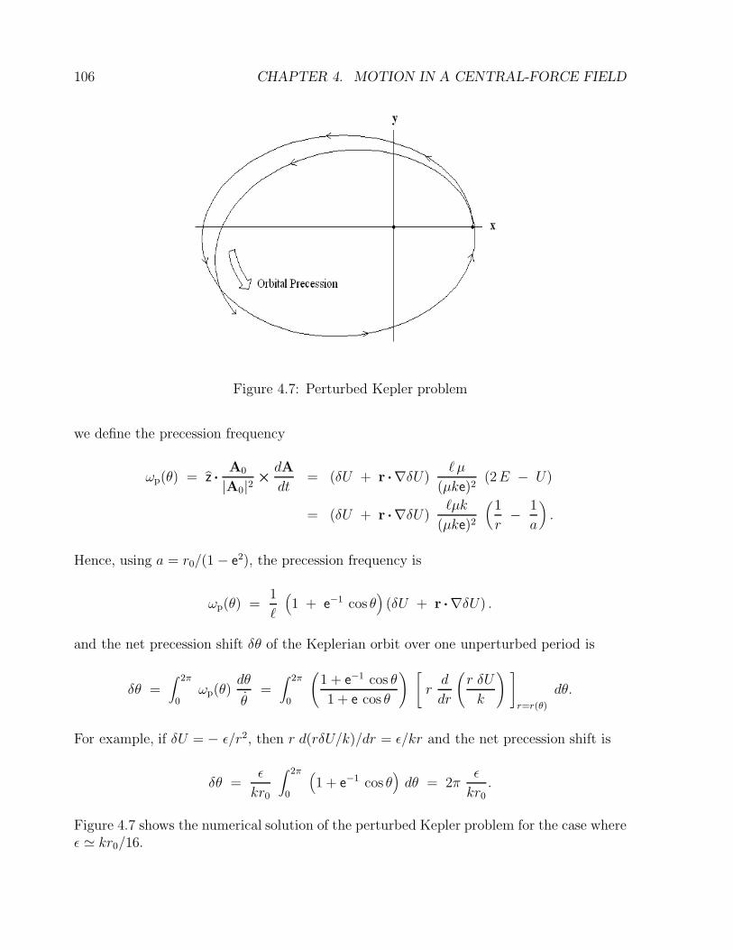
106 CHAPTER 4. MOTION IN A CENTRAL-FORCE FIELD
Figure 4.7: Perturbed Kepler problem
we define the precession frequency
ωp(θ) = z ·A0
|A0|2×dA
dt= (δU + r ·∇δU)
` µ
(µke)2(2E − U)
= (δU + r ·∇δU)`µk
(µke)2
(1
r− 1
a
).
Hence, using a = r0/(1 − e2), the precession frequency is
ωp(θ) =1
`
(1 + e−1 cos θ
)(δU + r ·∇δU) .
and the net precession shift δθ of the Keplerian orbit over one unperturbed period is
δθ =∫ 2π
0ωp(θ)
dθ
θ=
∫ 2π
0
(1 + e−1 cos θ
1 + e cos θ
) [
rd
dr
(r δU
k
) ]
r=r(θ)
dθ.
For example, if δU = − ε/r2, then r d(rδU/k)/dr = ε/kr and the net precession shift is
δθ =ε
kr0
∫ 2π
0
(1 + e−1 cos θ
)dθ = 2π
ε
kr0.
Figure 4.7 shows the numerical solution of the perturbed Kepler problem for the case whereε ' kr0/16.
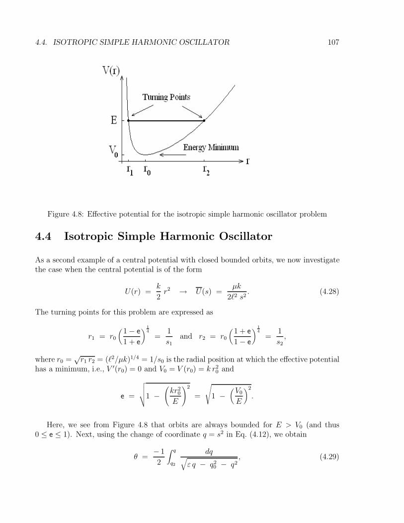
4.4. ISOTROPIC SIMPLE HARMONIC OSCILLATOR 107
Figure 4.8: Effective potential for the isotropic simple harmonic oscillator problem
4.4 Isotropic Simple Harmonic Oscillator
As a second example of a central potential with closed bounded orbits, we now investigatethe case when the central potential is of the form
U(r) =k
2r2 → U(s) =
µk
2`2 s2. (4.28)
The turning points for this problem are expressed as
r1 = r0
(1 − e
1 + e
)1
4
=1
s1
and r2 = r0
(1 + e
1 − e
)1
4
=1
s2
,
where r0 =√r1 r2 = (`2/µk)1/4 = 1/s0 is the radial position at which the effective potential
has a minimum, i.e., V ′(r0) = 0 and V0 = V (r0) = k r20 and
e =
√√√√1 −(kr2
0
E
)2
=
√
1 −(V0
E
)2
.
Here, we see from Figure 4.8 that orbits are always bounded for E > V0 (and thus0 ≤ e ≤ 1). Next, using the change of coordinate q = s2 in Eq. (4.12), we obtain
θ =− 1
2
∫ q
q2
dq√ε q − q2
0 − q2, (4.29)
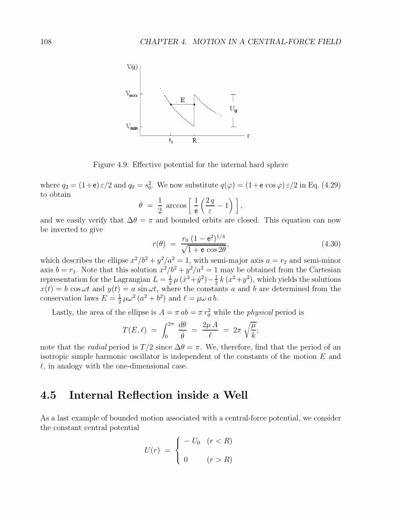
108 CHAPTER 4. MOTION IN A CENTRAL-FORCE FIELD
Figure 4.9: Effective potential for the internal hard sphere
where q2 = (1+e) ε/2 and q0 = s20. We now substitute q(ϕ) = (1+e cosϕ) ε/2 in Eq. (4.29)
to obtain
θ =1
2arccos
[1
e
(2 q
ε− 1
) ],
and we easily verify that ∆θ = π and bounded orbits are closed. This equation can nowbe inverted to give
r(θ) =r0 (1 − e2)1/4
√1 + e cos 2θ
, (4.30)
which describes the ellipse x2/b2 + y2/a2 = 1, with semi-major axis a = r2 and semi-minoraxis b = r1. Note that this solution x2/b2 + y2/a2 = 1 may be obtained from the Cartesianrepresentation for the Lagrangian L = 1
2µ (x2+y2)− 1
2k (x2+y2), which yields the solutions
x(t) = b cosωt and y(t) = a sinωt, where the constants a and b are determined from theconservation laws E = 1
2µω2 (a2 + b2) and ` = µω a b.
Lastly, the area of the ellipse is A = π ab = π r20 while the physical period is
T (E, `) =∫ 2π
0
dθ
θ=
2µA
`= 2π
õ
k;
note that the radial period is T/2 since ∆θ = π. We, therefore, find that the period of anisotropic simple harmonic oscillator is independent of the constants of the motion E and`, in analogy with the one-dimensional case.
4.5 Internal Reflection inside a Well
As a last example of bounded motion associated with a central-force potential, we considerthe constant central potential
U(r) =
− U0 (r < R)
0 (r > R)
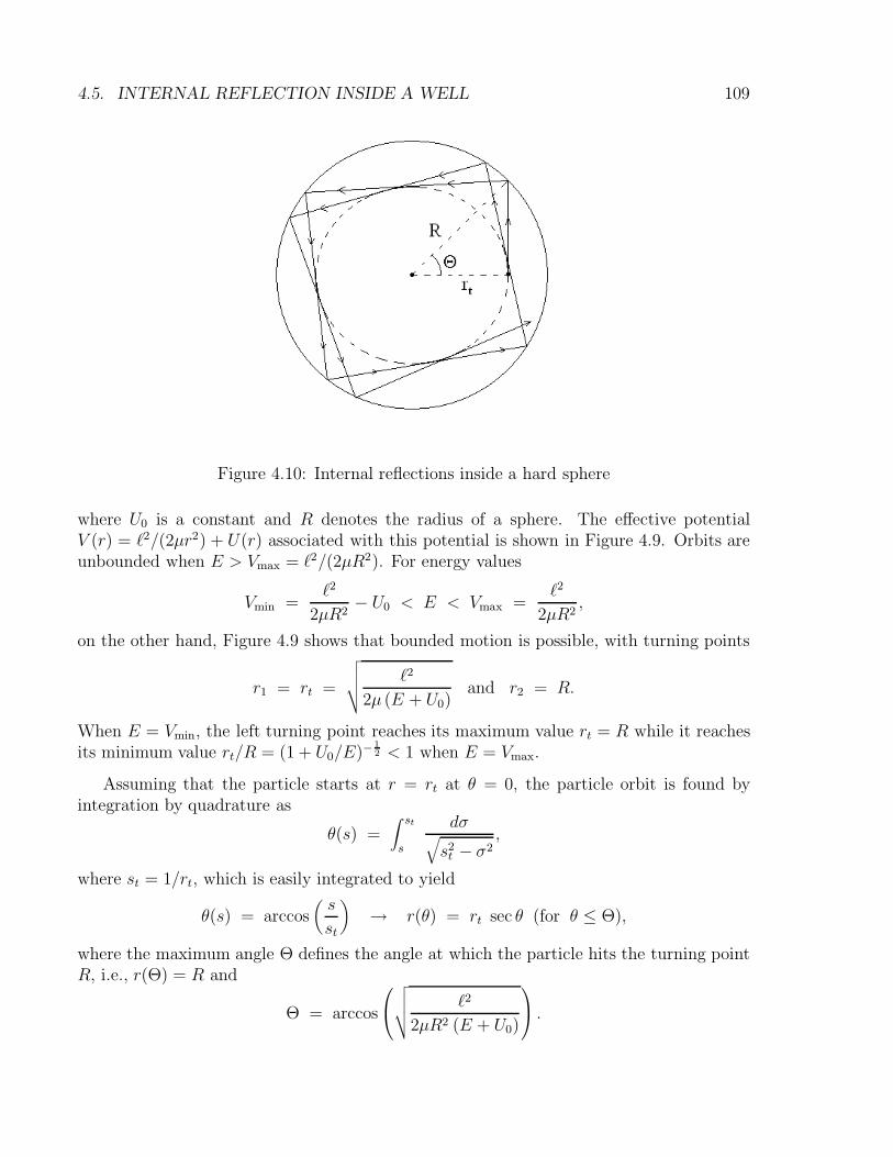
4.5. INTERNAL REFLECTION INSIDE A WELL 109
Figure 4.10: Internal reflections inside a hard sphere
where U0 is a constant and R denotes the radius of a sphere. The effective potentialV (r) = `2/(2µr2) + U(r) associated with this potential is shown in Figure 4.9. Orbits areunbounded when E > Vmax = `2/(2µR2). For energy values
Vmin =`2
2µR2− U0 < E < Vmax =
`2
2µR2,
on the other hand, Figure 4.9 shows that bounded motion is possible, with turning points
r1 = rt =
√√√√ `2
2µ (E + U0)and r2 = R.
When E = Vmin, the left turning point reaches its maximum value rt = R while it reachesits minimum value rt/R = (1 + U0/E)−
1
2 < 1 when E = Vmax.
Assuming that the particle starts at r = rt at θ = 0, the particle orbit is found byintegration by quadrature as
θ(s) =∫ st
s
dσ√s2t − σ2
,
where st = 1/rt, which is easily integrated to yield
θ(s) = arccos(s
st
)→ r(θ) = rt sec θ (for θ ≤ Θ),
where the maximum angle Θ defines the angle at which the particle hits the turning pointR, i.e., r(Θ) = R and
Θ = arccos
√√√√ `2
2µR2 (E + U0)
.
110 CHAPTER 4. MOTION IN A CENTRAL-FORCE FIELD
Subsequent motion of the particle involves an infinite sequence of internal reflections asshown in Figure 4.10. The case where E > `2/2µR2 involves a single turning point and isdiscussed in Sec. 5.6.2.
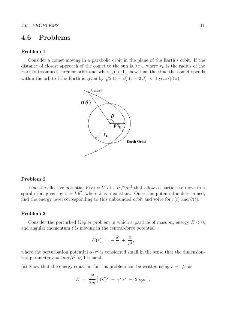
4.6. PROBLEMS 111
4.6 Problems
Problem 1
Consider a comet moving in a parabolic orbit in the plane of the Earth’s orbit. If thedistance of closest approach of the comet to the sun is β rE , where rE is the radius of theEarth’s (assumed) circular orbit and where β < 1, show that the time the comet spends
within the orbit of the Earth is given by√
2 (1 − β) (1 + 2β) × 1 year/(3π).
Problem 2
Find the effective potential V (r) = U(r) + `2/2µr2 that allows a particle to move in aspiral orbit given by r = k θ2, where k is a constant. Once this potential is determined,find the energy level corresponding to this unbounded orbit and solve for r(t) and θ(t).
Problem 3
Consider the perturbed Kepler problem in which a particle of mass m, energy E < 0,and angular momentum ` is moving in the central-force potential
U(r) = − k
r+
α
r2,
where the perturbation potential α/r2 is considered small in the sense that the dimension-less parameter ε = 2mα/`2 1 is small.
(a) Show that the energy equation for this problem can be written using s = 1/r as
E =`2
2m
[(s′)2 + γ2 s2 − 2 s0s
],

112 CHAPTER 4. MOTION IN A CENTRAL-FORCE FIELD
where s0 = mk/`2 and γ2 = 1 + ε.
(b) Show that the turning points are
s1 =s0
γ2(1 − e) and s2 =
s0
γ2(1 + e),
where e =√
1 + 2 γ2`2E/mk2.
(c) By solving the integral
θ(s) = −∫ s
s2
dσ√
(2mE/`2) + 2 s0σ − γ2 σ2,
where θ(s2) = 0, show that
r(θ) =γ2 r0
1 + e cos(γθ),
where r0 = 1/s0.
Problem 4
A Keplerian elliptical orbit, described by the relation r(θ) = r0/(1+ e cos θ), undergoesa precession motion when perturbed by the perturbation potential δU(r), with precessionfrequency
ωp(θ) = z ·dA
dt×
A
|A|2 = − 1
`
(1 + e−1 cos θ
)(δU + r ·∇δU)
where A = p× L−µk r denotes the Laplace-Runge-Lenz vector for the unperturbed Keplerproblem.
Show that the net precession shift δθ of the Keplerian orbit over one unperturbed periodis
δθ =∫ 2π
0ωp(θ)
dθ
θ= − 6π
α
kr20
.
if the perturbation potential is δU(r) = −α/r3, where α is a constant.
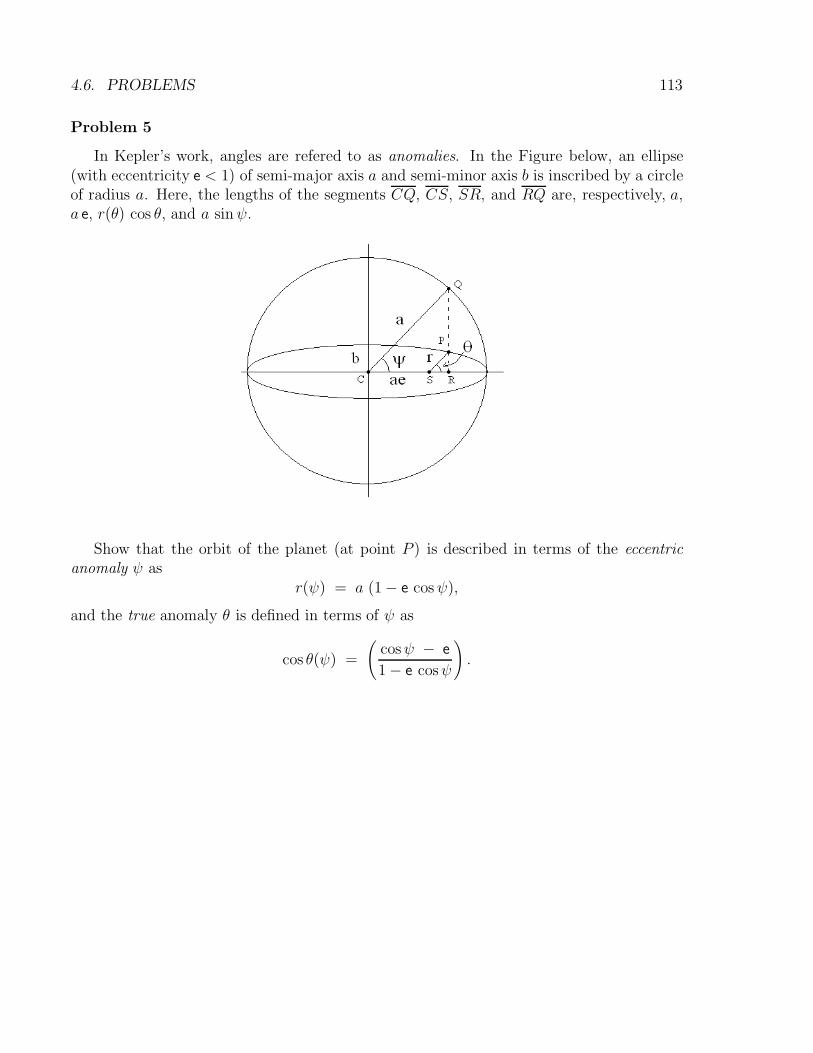
4.6. PROBLEMS 113
Problem 5
In Kepler’s work, angles are refered to as anomalies. In the Figure below, an ellipse(with eccentricity e < 1) of semi-major axis a and semi-minor axis b is inscribed by a circleof radius a. Here, the lengths of the segments CQ, CS, SR, and RQ are, respectively, a,a e, r(θ) cos θ, and a sinψ.
Show that the orbit of the planet (at point P ) is described in terms of the eccentricanomaly ψ as
r(ψ) = a (1 − e cosψ),
and the true anomaly θ is defined in terms of ψ as
cos θ(ψ) =
(cosψ − e
1 − e cosψ
)
.
114 CHAPTER 4. MOTION IN A CENTRAL-FORCE FIELD
Chapter 5
Collisions and Scattering Theory
In the previous Chapter, we investigated two types of orbits (bounded and unbounded)for two-particle systems evolving under the influence of a central potential. In the presentChapter, we focus our attention on unbounded orbits within the context of elastic collisiontheory. In this context, a collision between two interacting particles involves a three-stepprocess: Step I – two particles are initially infinitely far apart (in which case, the energy ofeach particle is assumed to be strictly kinetic); Step II – as the two particles approach eachother, their interacting potential (repulsive or attractive) causes them to reach a distanceof closest approach; and Step III – the two particles then move progressively farther apart(eventually reaching a point where the energy of each particle is once again strictly kinetic).
These three steps form the foundations of Collision Kinematics and Collision Dynamics.The topic of Collision Kinematics, which describes the collision in terms of the conservationlaws of momentum and energy, deals with Steps I and III; here, the incoming particlesdefine the initial state of the two-particle system while the outgoing particles define thefinal state. The topic of Collision Dynamics, on the other hand, deals with Step II, inwhich the particular nature of the interaction is taken into account.
5.1 Two-Particle Collisions in the LAB Frame
Consider the collision of two particles (labeled 1 and 2) of masses m1 and m2, respectively.Let us denote the velocities of particles 1 and 2 before the collision as u1 and u2, respectively,while the velocities after the collision are denoted v1 and v2. Furthermore, the particlemomenta before and after the collision are denoted p and q, respectively.
To simplify the analysis, we define the laboratory (LAB) frame to correspond to thereference frame in which m2 is at rest (i.e., u2 = 0); in this collision scenario, m1 acts asthe projectile particle and m2 is the target particle. We now write the velocities u1, v1, and
115
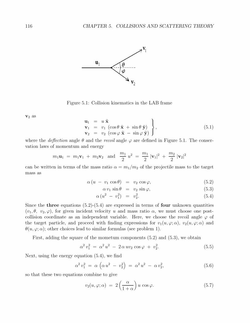
116 CHAPTER 5. COLLISIONS AND SCATTERING THEORY
Figure 5.1: Collision kinematics in the LAB frame
v2 asu1 = u x
v1 = v1 (cos θ x + sin θ y)v2 = v2 (cosϕ x − sinϕ y)
, (5.1)
where the deflection angle θ and the recoil angle ϕ are defined in Figure 5.1. The conser-vation laws of momentum and energy
m1u1 = m1v1 + m2v2 andm1
2u2 =
m1
2|v1|2 +
m2
2|v2|2
can be written in terms of the mass ratio α = m1/m2 of the projectile mass to the targetmass as
α (u − v1 cos θ) = v2 cosϕ, (5.2)
αv1 sin θ = v2 sinϕ, (5.3)
α (u2 − v21) = v2
2. (5.4)
Since the three equations (5.2)-(5.4) are expressed in terms of four unknown quantities(v1, θ, v2, ϕ), for given incident velocity u and mass ratio α, we must choose one post-collision coordinate as an independent variable. Here, we choose the recoil angle ϕ ofthe target particle, and proceed with finding expressions for v1(u, ϕ;α), v2(u, ϕ;α) andθ(u, ϕ;α); other choices lead to similar formulas (see problem 1).
First, adding the square of the mometum components (5.2) and (5.3), we obtain
α2 v21 = α2 u2 − 2α uv2 cosϕ + v2
2. (5.5)
Next, using the energy equation (5.4), we find
α2 v21 = α
(αu2 − v2
2
)= α2 u2 − α v2
2, (5.6)
so that these two equations combine to give
v2(u, ϕ;α) = 2(
α
1 + α
)u cosϕ. (5.7)
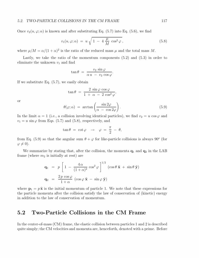
5.2. TWO-PARTICLE COLLISIONS IN THE CM FRAME 117
Once v2(u, ϕ;α) is known and after substituting Eq. (5.7) into Eq. (5.6), we find
v1(u, ϕ;α) = u
√1 − 4
µ
Mcos2 ϕ , (5.8)
where µ/M = α/(1 + α)2 is the ratio of the reduced mass µ and the total mass M .
Lastly, we take the ratio of the momentum components (5.2) and (5.3) in order toeliminate the unknown v1 and find
tan θ =v2 sinϕ
αu − v2 cosϕ.
If we substitute Eq. (5.7), we easily obtain
tan θ =2 sinϕ cosϕ
1 + α − 2 cos2 ϕ,
or
θ(ϕ;α) = arctan
(sin 2ϕ
α − cos 2ϕ
)
. (5.9)
In the limit α = 1 (i.e., a collision involving identical particles), we find v2 = u cosϕ andv1 = u sinϕ from Eqs. (5.7) and (5.8), respectively, and
tan θ = cotϕ → ϕ =π
2− θ,
from Eq. (5.9) so that the angular sum θ + ϕ for like-particle collisions is always 90o (forϕ 6= 0).
We summarize by stating that, after the collision, the momenta q1 and q2 in the LABframe (where m2 is initially at rest) are
q1 = p
[
1 − 4α
(1 + α)2cos2 ϕ
]1/2
(cos θ x + sin θ y)
q2 =2 p cosϕ
1 + α(cosϕ x − sinϕ y)
where p1 = p x is the initial momentum of particle 1. We note that these expressions forthe particle momenta after the collision satisfy the law of conservation of (kinetic) energyin addition to the law of conservation of momentum.
5.2 Two-Particle Collisions in the CM Frame
In the center-of-mass (CM) frame, the elastic collision between particles 1 and 2 is describedquite simply; the CM velocities and momenta are, henceforth, denoted with a prime. Before
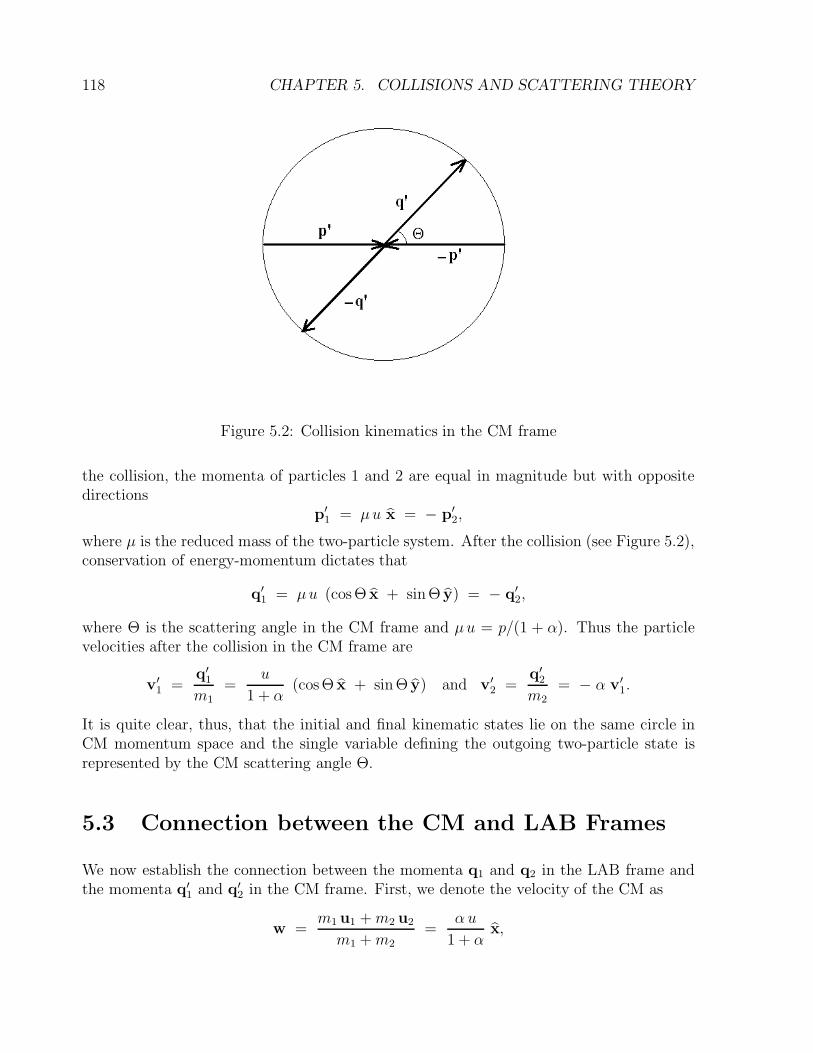
118 CHAPTER 5. COLLISIONS AND SCATTERING THEORY
Figure 5.2: Collision kinematics in the CM frame
the collision, the momenta of particles 1 and 2 are equal in magnitude but with oppositedirections
p′1 = µu x = − p′
2,
where µ is the reduced mass of the two-particle system. After the collision (see Figure 5.2),conservation of energy-momentum dictates that
q′1 = µu (cosΘ x + sinΘ y) = − q′
2,
where Θ is the scattering angle in the CM frame and µu = p/(1 + α). Thus the particlevelocities after the collision in the CM frame are
v′1 =
q′1
m1=
u
1 + α(cosΘ x + sinΘ y) and v′
2 =q′
2
m2= − α v′
1.
It is quite clear, thus, that the initial and final kinematic states lie on the same circle inCM momentum space and the single variable defining the outgoing two-particle state isrepresented by the CM scattering angle Θ.
5.3 Connection between the CM and LAB Frames
We now establish the connection between the momenta q1 and q2 in the LAB frame andthe momenta q′
1 and q′2 in the CM frame. First, we denote the velocity of the CM as
w =m1 u1 +m2 u2
m1 +m2
=α u
1 + αx,
5.3. CONNECTION BETWEEN THE CM AND LAB FRAMES 119
Figure 5.3: CM collision geometry
so that w = |w| = α u/(1 + α) and |v′2| = w = α |v′
1|.The connection between v′
1 and v1 is expressed as
v′1 = v1 − w →
v1 cos θ = w (1 + α−1 cosΘ)
v1 sin θ = wα−1 sinΘ
so that
tan θ =sinΘ
α+ cos Θ, (5.10)
andv1 = v′1
√1 + α2 + 2α cosΘ,
where v′1 = u/(1 + α). Likewise, the connection between v′2 and v2 is expressed as
v′2 = v2 − w →
v2 cosϕ = w (1 − cos Θ)
v2 sinϕ = w sinΘ
so that
tanϕ =sinΘ
1 − cos Θ= cot
Θ
2→ ϕ =
1
2(π − Θ),
and
v2 = 2 v′2 sinΘ
2,
where v′2 = α u/(1 + α) = w.
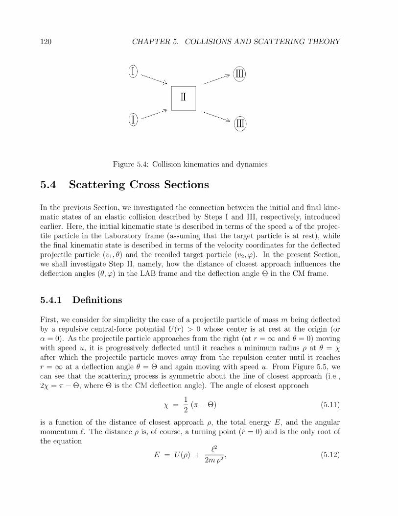
120 CHAPTER 5. COLLISIONS AND SCATTERING THEORY
Figure 5.4: Collision kinematics and dynamics
5.4 Scattering Cross Sections
In the previous Section, we investigated the connection between the initial and final kine-matic states of an elastic collision described by Steps I and III, respectively, introducedearlier. Here, the initial kinematic state is described in terms of the speed u of the projec-tile particle in the Laboratory frame (assuming that the target particle is at rest), whilethe final kinematic state is described in terms of the velocity coordinates for the deflectedprojectile particle (v1, θ) and the recoiled target particle (v2, ϕ). In the present Section,we shall investigate Step II, namely, how the distance of closest approach influences thedeflection angles (θ, ϕ) in the LAB frame and the deflection angle Θ in the CM frame.
5.4.1 Definitions
First, we consider for simplicity the case of a projectile particle of mass m being deflectedby a repulsive central-force potential U(r) > 0 whose center is at rest at the origin (orα = 0). As the projectile particle approaches from the right (at r = ∞ and θ = 0) movingwith speed u, it is progressively deflected until it reaches a minimum radius ρ at θ = χafter which the projectile particle moves away from the repulsion center until it reachesr = ∞ at a deflection angle θ = Θ and again moving with speed u. From Figure 5.5, wecan see that the scattering process is symmetric about the line of closest approach (i.e.,2χ = π − Θ, where Θ is the CM deflection angle). The angle of closest approach
χ =1
2(π − Θ) (5.11)
is a function of the distance of closest approach ρ, the total energy E, and the angularmomentum `. The distance ρ is, of course, a turning point (r = 0) and is the only root ofthe equation
E = U(ρ) +`2
2mρ2, (5.12)
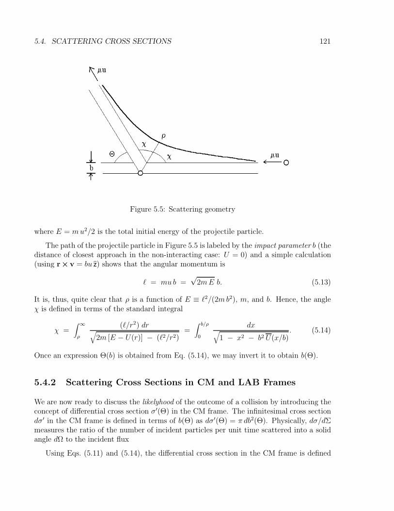
5.4. SCATTERING CROSS SECTIONS 121
Figure 5.5: Scattering geometry
where E = mu2/2 is the total initial energy of the projectile particle.
The path of the projectile particle in Figure 5.5 is labeled by the impact parameter b (thedistance of closest approach in the non-interacting case: U = 0) and a simple calculation(using r×v = bu z) shows that the angular momentum is
` = mub =√
2mE b. (5.13)
It is, thus, quite clear that ρ is a function of E ≡ `2/(2mb2), m, and b. Hence, the angleχ is defined in terms of the standard integral
χ =∫ ∞
ρ
(`/r2) dr√
2m [E − U(r)] − (`2/r2)=∫ b/ρ
0
dx√
1 − x2 − b2 U(x/b). (5.14)
Once an expression Θ(b) is obtained from Eq. (5.14), we may invert it to obtain b(Θ).
5.4.2 Scattering Cross Sections in CM and LAB Frames
We are now ready to discuss the likelyhood of the outcome of a collision by introducing theconcept of differential cross section σ′(Θ) in the CM frame. The infinitesimal cross sectiondσ′ in the CM frame is defined in terms of b(Θ) as dσ′(Θ) = π db2(Θ). Physically, dσ/dΣmeasures the ratio of the number of incident particles per unit time scattered into a solidangle dΩ to the incident flux
Using Eqs. (5.11) and (5.14), the differential cross section in the CM frame is defined
122 CHAPTER 5. COLLISIONS AND SCATTERING THEORY
as
σ′(Θ) =dσ′
2π sinΘ dΘ=
b(Θ)
sinΘ
∣∣∣∣∣db(Θ)
dΘ
∣∣∣∣∣ , (5.15)
and the total cross section is, thus, defined as
σT = 2π∫ π
0σ′(Θ) sinΘ dΘ.
We note that, in Eq. (5.15), the quantity db/dΘ is often negative and, thus, we must takeits absolute value to ensure that σ′(Θ) is positive.
The differential cross section can also be written in the LAB frame in terms of thedeflection angle θ as
σ(θ) =dσ
2π sin θ dθ=
b(θ)
sin θ
∣∣∣∣∣db(θ)
dθ
∣∣∣∣∣ . (5.16)
Since the infinitesimal cross section dσ = dσ′ is the same in both frames (i.e., the likelyhoodof a collision should not depend on the choice of a frame of reference), we find
σ(θ) sin θ dθ = σ′(Θ) sinΘ dΘ,
from which we obtain
σ(θ) = σ′(Θ)sinΘ
sin θ
dΘ
dθ, (5.17)
or
σ′(Θ) = σ(θ)sin θ
sinΘ
dθ
dΘ. (5.18)
Eq. (5.17) yields an expression for the differential cross section in the LAB frame σ(θ) oncethe differential cross section in the CM frame σ′(Θ) and an explicit formula for Θ(θ) are
known. Eq. (5.18) represents the inverse transformation σ(θ) → σ′(Θ). We point outthat, whereas the CM differential cross section σ′(Θ) is naturally associated with theo-retical calculations, the LAB differential cross section σ(θ) is naturally associated withexperimental measurements. Hence, the transformation (5.17) is used to translate a theo-retical prediction into an observable experimental cross section, while the transformation(5.18) is used to translate experimental measurements into a format suitable for theoreticalanalysis.
We note that these transformations rely on finding relations between the LAB deflectionangle θ and the CM deflection angle Θ given by Eq. (5.10), which can be converted into
sin(Θ − θ) = α sin θ. (5.19)
For example, using these relations, we now show how to obtain an expression for Eq. (5.17)by using Eqs. (5.10) and (5.19). First, we use Eq. (5.19) to obtain
dΘ
dθ=
α cos θ + cos(Θ − θ)
cos(Θ − θ), (5.20)
5.5. RUTHERFORD SCATTERING 123
where
cos(Θ − θ) =√
1 − α2 sin2 θ .
Next, using Eq. (5.10), we show that
sinΘ
sin θ=
α+ cos Θ
cos θ=
α + [cos(Θ − θ) cos θ −= α sin θ︷ ︸︸ ︷
sin(Θ − θ) sin θ]
cos θ
=α (1 − sin2 θ) + cos(Θ − θ) cos θ
cos θ= α cos θ +
√1 − α2 sin2 θ . (5.21)
Thus by combining Eqs. (5.20) and (5.21), we find
sinΘ
sin θ
dΘ
dθ=
[α cos θ +√
1 − α2 sin2 θ]2√1 − α2 sin2 θ
= 2α cos θ +1 + α2 cos 2θ√1 − α2 sin2 θ
, (5.22)
which is valid for α < 1. Lastly, noting from Eq. (5.19), that the CM deflection angle isdefined as
Θ(θ) = θ + arcsin(α sin θ ),
the transformation σ′(Θ) → σ(θ) is now complete. Similar manipulations yield the trans-formation σ(θ) → σ′(Θ). We note that the LAB-frame cross section σ(θ) are generallydifficult to obtain for arbitrary mass ratio α = m1/m2.
5.5 Rutherford Scattering
As an explicit example of the scattering formalism developed in this Chapter, we investigatethe scattering of a charged particle of mass m1 and charge q1 by another charged particleof mass m2 m1 and charge q2 such that q1 q2 > 0 and µ ' m1. This situation leads tothe two particles experiencing a repulsive central force with potential
U(r) =k
r,
where k = q1q2/(4π ε0) > 0.
The turning-point equation in this case is
E = Eb2
ρ2+
k
ρ,
whose solution is the distance of closest approach
ρ = r0 +√r20 + b2 = b
(ε +
√1 + ε2
), (5.23)
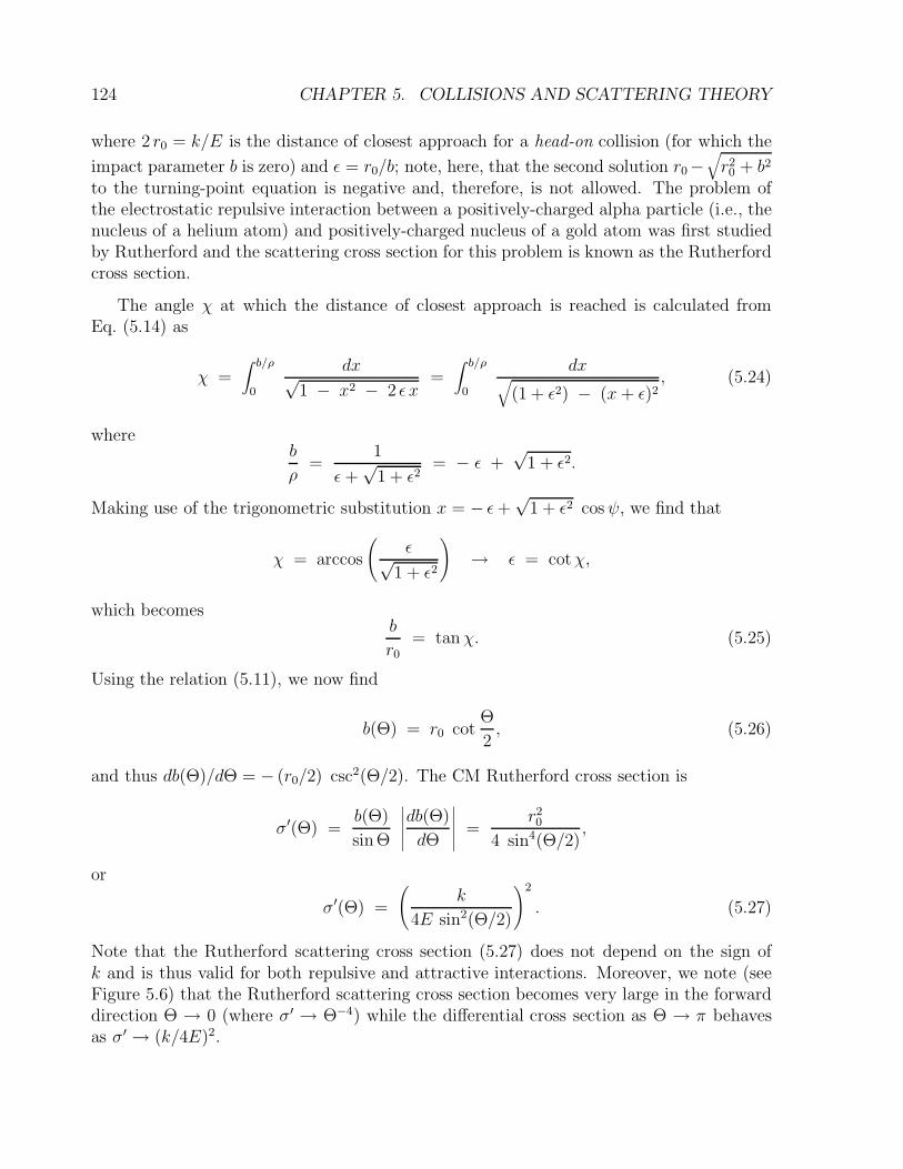
124 CHAPTER 5. COLLISIONS AND SCATTERING THEORY
where 2 r0 = k/E is the distance of closest approach for a head-on collision (for which the
impact parameter b is zero) and ε = r0/b; note, here, that the second solution r0−√r20 + b2
to the turning-point equation is negative and, therefore, is not allowed. The problem ofthe electrostatic repulsive interaction between a positively-charged alpha particle (i.e., thenucleus of a helium atom) and positively-charged nucleus of a gold atom was first studiedby Rutherford and the scattering cross section for this problem is known as the Rutherfordcross section.
The angle χ at which the distance of closest approach is reached is calculated fromEq. (5.14) as
χ =∫ b/ρ
0
dx√1 − x2 − 2 ε x
=∫ b/ρ
0
dx√
(1 + ε2) − (x+ ε)2, (5.24)
whereb
ρ=
1
ε+√
1 + ε2= − ε +
√1 + ε2.
Making use of the trigonometric substitution x = − ε+√
1 + ε2 cosψ, we find that
χ = arccos
(ε√
1 + ε2
)
→ ε = cotχ,
which becomesb
r0= tanχ. (5.25)
Using the relation (5.11), we now find
b(Θ) = r0 cotΘ
2, (5.26)
and thus db(Θ)/dΘ = − (r0/2) csc2(Θ/2). The CM Rutherford cross section is
σ′(Θ) =b(Θ)
sinΘ
∣∣∣∣∣db(Θ)
dΘ
∣∣∣∣∣ =r20
4 sin4(Θ/2),
or
σ′(Θ) =
(k
4E sin2(Θ/2)
)2
. (5.27)
Note that the Rutherford scattering cross section (5.27) does not depend on the sign ofk and is thus valid for both repulsive and attractive interactions. Moreover, we note (seeFigure 5.6) that the Rutherford scattering cross section becomes very large in the forwarddirection Θ → 0 (where σ′ → Θ−4) while the differential cross section as Θ → π behavesas σ′ → (k/4E)2.
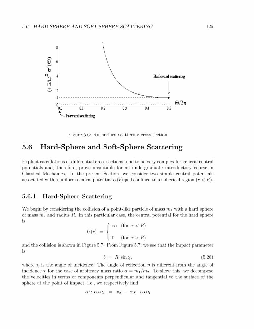
5.6. HARD-SPHERE AND SOFT-SPHERE SCATTERING 125
Figure 5.6: Rutherford scattering cross-section
5.6 Hard-Sphere and Soft-Sphere Scattering
Explicit calculations of differential cross sections tend to be very complex for general centralpotentials and, therefore, prove unsuitable for an undergraduate introductory course inClassical Mechanics. In the present Section, we consider two simple central potentialsassociated with a uniform central potential U(r) 6= 0 confined to a spherical region (r < R).
5.6.1 Hard-Sphere Scattering
We begin by considering the collision of a point-like particle of mass m1 with a hard sphereof mass m2 and radius R. In this particular case, the central potential for the hard sphereis
U(r) =
∞ (for r < R)
0 (for r > R)
and the collision is shown in Figure 5.7. From Figure 5.7, we see that the impact parameteris
b = R sinχ, (5.28)
where χ is the angle of incidence. The angle of reflection η is different from the angle ofincidence χ for the case of arbitrary mass ratio α = m1/m2. To show this, we decomposethe velocities in terms of components perpendicular and tangential to the surface of thesphere at the point of impact, i.e., we respectively find
αu cosχ = v2 − α v1 cos η
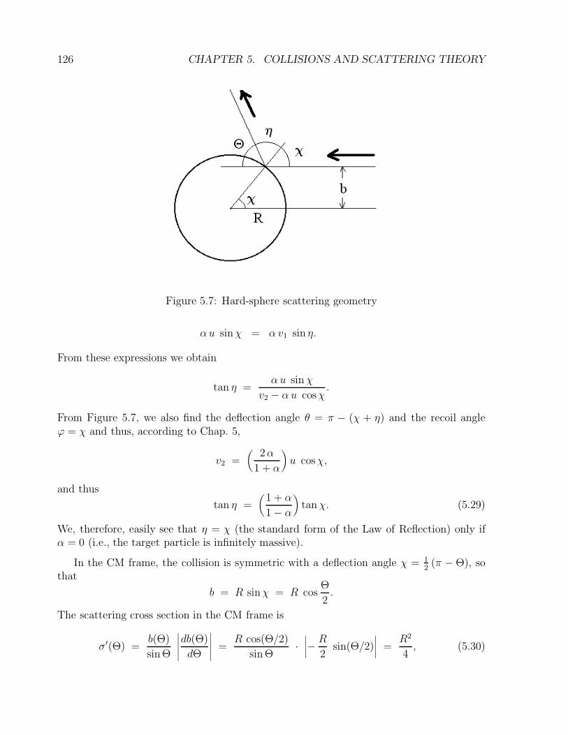
126 CHAPTER 5. COLLISIONS AND SCATTERING THEORY
Figure 5.7: Hard-sphere scattering geometry
αu sinχ = α v1 sin η.
From these expressions we obtain
tan η =α u sinχ
v2 − α u cosχ.
From Figure 5.7, we also find the deflection angle θ = π − (χ + η) and the recoil angleϕ = χ and thus, according to Chap. 5,
v2 =(
2α
1 + α
)u cosχ,
and thus
tan η =(
1 + α
1 − α
)tanχ. (5.29)
We, therefore, easily see that η = χ (the standard form of the Law of Reflection) only ifα = 0 (i.e., the target particle is infinitely massive).
In the CM frame, the collision is symmetric with a deflection angle χ = 12(π − Θ), so
that
b = R sinχ = R cosΘ
2.
The scattering cross section in the CM frame is
σ′(Θ) =b(Θ)
sinΘ
∣∣∣∣∣db(Θ)
dΘ
∣∣∣∣∣ =R cos(Θ/2)
sinΘ·∣∣∣∣−
R
2sin(Θ/2)
∣∣∣∣ =R2
4, (5.30)
5.6. HARD-SPHERE AND SOFT-SPHERE SCATTERING 127
and the total cross section is
σT = 2π∫ π
0σ′(Θ) sin Θ dΘ = π R2, (5.31)
i.e., the total cross section for the problem of hard-sphere collision is equal to the effectivearea of the sphere.
The scattering cross section in the LAB frame can also be obtained for the case α < 1using Eqs. (5.17) and (5.22) as
σ(θ) =R2
4
(
2α cos θ +1 + α2 cos 2θ√1 − α2 sin2 θ
)
, (5.32)
for α = m1/m2 < 1. The integration of this formula must yield the total cross section
σT = 2π∫ π
0σ(θ) sin θ dθ,
where θmax = π for α < 1.
5.6.2 Soft-Sphere Scattering
We now consider the scattering of a particle subjected to the attractive potential consideredin Sec. 4.5
U(r) =
− U0 (for r < R)
0 for r > R(5.33)
where the constant U0 denotes the depth of the attractive potential well and E > `2/2µR2
involves a single turning point. We denote β the angle at which the incoming particle entersthe soft-sphere potential (see Figure 5.8), and thus the impact parameter b of the incomingparticle is b = R sin β. The particle enters the soft-sphere potential region (r < R) andreaches a distance of closest approach ρ, defined from the turning-point condition
E = −U0 + Eb2
ρ2→ ρ =
b√
1 + U0/E=
R
nsinβ,
where n =√
1 + U0/E denotes the index of refraction of the soft-sphere potential region.From Figure 5.8, we note that an optical analogy helps us determine that, through Snell’slaw, we find
sinβ = n sin(β − Θ
2
), (5.34)
where the transmission angle α is given in terms of the incident angle β and the CMscattering angle −Θ as Θ = 2 (β − α).
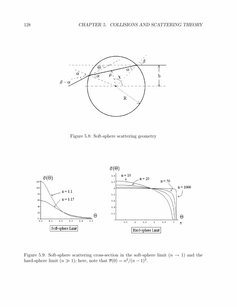
128 CHAPTER 5. COLLISIONS AND SCATTERING THEORY
Figure 5.8: Soft-sphere scattering geometry
Figure 5.9: Soft-sphere scattering cross-section in the soft-sphere limit (n → 1) and thehard-sphere limit (n 1); here, note that σ(0) = n2/(n − 1)2.
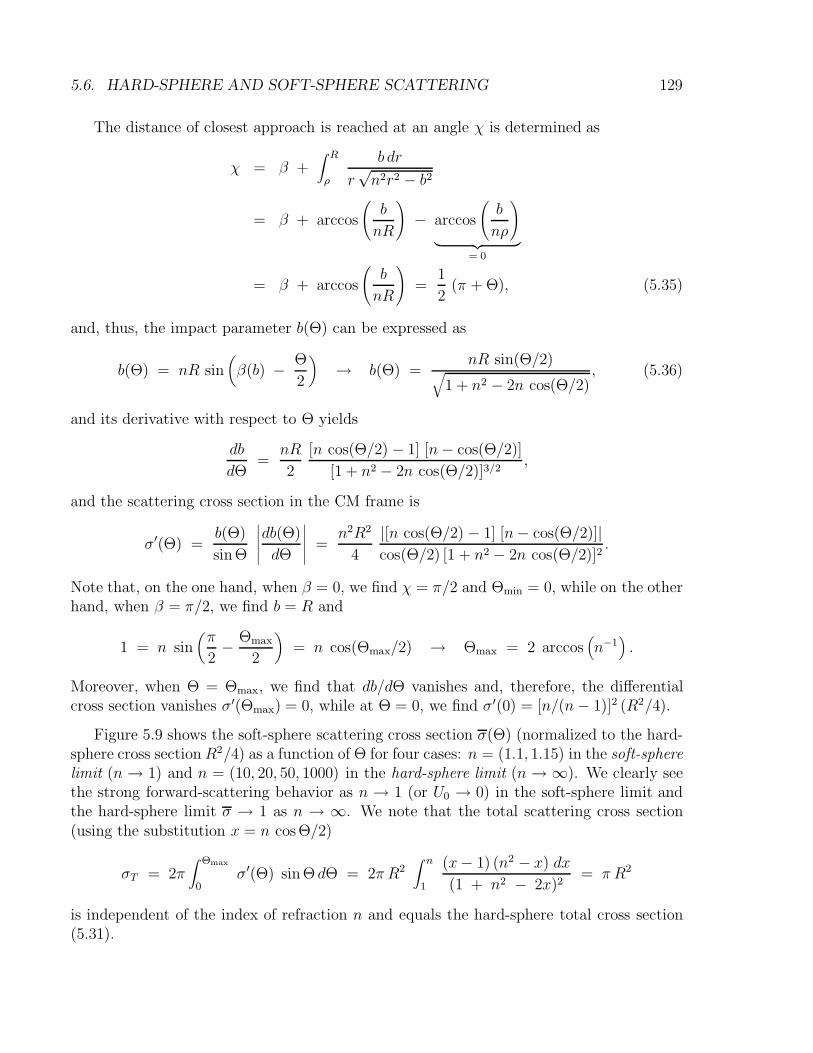
5.6. HARD-SPHERE AND SOFT-SPHERE SCATTERING 129
The distance of closest approach is reached at an angle χ is determined as
χ = β +∫ R
ρ
b dr
r√n2r2 − b2
= β + arccos
(b
nR
)
− arccos
(b
nρ
)
︸ ︷︷ ︸= 0
= β + arccos
(b
nR
)
=1
2(π + Θ), (5.35)
and, thus, the impact parameter b(Θ) can be expressed as
b(Θ) = nR sin(β(b) − Θ
2
)→ b(Θ) =
nR sin(Θ/2)√
1 + n2 − 2n cos(Θ/2), (5.36)
and its derivative with respect to Θ yields
db
dΘ=
nR
2
[n cos(Θ/2) − 1] [n− cos(Θ/2)]
[1 + n2 − 2n cos(Θ/2)]3/2,
and the scattering cross section in the CM frame is
σ′(Θ) =b(Θ)
sinΘ
∣∣∣∣∣db(Θ)
dΘ
∣∣∣∣∣ =n2R2
4
|[n cos(Θ/2) − 1] [n− cos(Θ/2)]|cos(Θ/2) [1 + n2 − 2n cos(Θ/2)]2
.
Note that, on the one hand, when β = 0, we find χ = π/2 and Θmin = 0, while on the otherhand, when β = π/2, we find b = R and
1 = n sin(π
2− Θmax
2
)= n cos(Θmax/2) → Θmax = 2 arccos
(n−1
).
Moreover, when Θ = Θmax, we find that db/dΘ vanishes and, therefore, the differentialcross section vanishes σ′(Θmax) = 0, while at Θ = 0, we find σ′(0) = [n/(n− 1)]2 (R2/4).
Figure 5.9 shows the soft-sphere scattering cross section σ(Θ) (normalized to the hard-sphere cross sectionR2/4) as a function of Θ for four cases: n = (1.1, 1.15) in the soft-spherelimit (n → 1) and n = (10, 20, 50, 1000) in the hard-sphere limit (n → ∞). We clearly seethe strong forward-scattering behavior as n → 1 (or U0 → 0) in the soft-sphere limit andthe hard-sphere limit σ → 1 as n → ∞. We note that the total scattering cross section(using the substitution x = n cosΘ/2)
σT = 2π∫ Θmax
0σ′(Θ) sinΘ dΘ = 2π R2
∫ n
1
(x− 1) (n2 − x) dx
(1 + n2 − 2x)2= π R2
is independent of the index of refraction n and equals the hard-sphere total cross section(5.31).
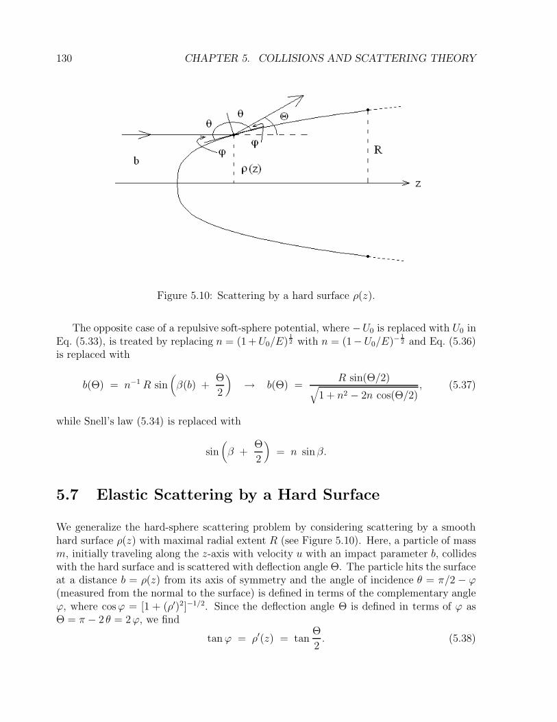
130 CHAPTER 5. COLLISIONS AND SCATTERING THEORY
Figure 5.10: Scattering by a hard surface ρ(z).
The opposite case of a repulsive soft-sphere potential, where −U0 is replaced with U0 inEq. (5.33), is treated by replacing n = (1 +U0/E)
1
2 with n = (1−U0/E)−1
2 and Eq. (5.36)is replaced with
b(Θ) = n−1 R sin(β(b) +
Θ
2
)→ b(Θ) =
R sin(Θ/2)√
1 + n2 − 2n cos(Θ/2), (5.37)
while Snell’s law (5.34) is replaced with
sin(β +
Θ
2
)= n sinβ.
5.7 Elastic Scattering by a Hard Surface
We generalize the hard-sphere scattering problem by considering scattering by a smoothhard surface ρ(z) with maximal radial extent R (see Figure 5.10). Here, a particle of massm, initially traveling along the z-axis with velocity u with an impact parameter b, collideswith the hard surface and is scattered with deflection angle Θ. The particle hits the surfaceat a distance b = ρ(z) from its axis of symmetry and the angle of incidence θ = π/2 − ϕ(measured from the normal to the surface) is defined in terms of the complementary angleϕ, where cosϕ = [1 + (ρ′)2]−1/2. Since the deflection angle Θ is defined in terms of ϕ asΘ = π − 2 θ = 2ϕ, we find
tanϕ = ρ′(z) = tanΘ
2. (5.38)
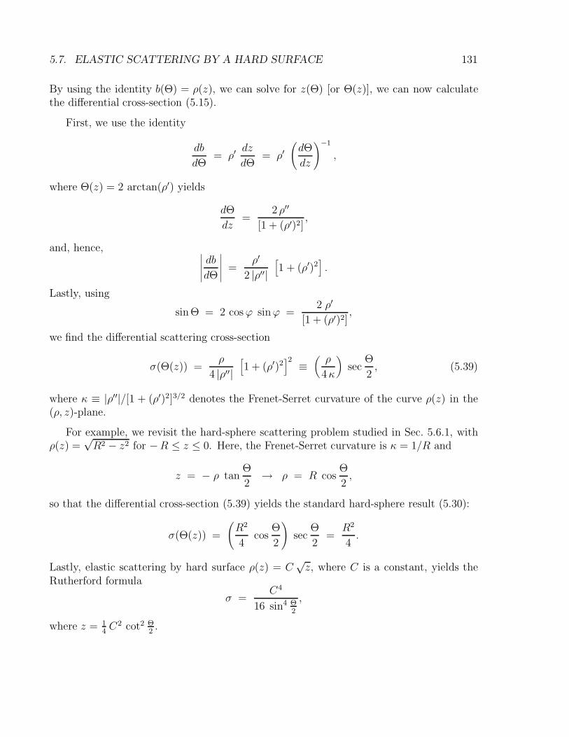
5.7. ELASTIC SCATTERING BY A HARD SURFACE 131
By using the identity b(Θ) = ρ(z), we can solve for z(Θ) [or Θ(z)], we can now calculatethe differential cross-section (5.15).
First, we use the identity
db
dΘ= ρ′
dz
dΘ= ρ′
(dΘ
dz
)−1
,
where Θ(z) = 2 arctan(ρ′) yields
dΘ
dz=
2 ρ′′
[1 + (ρ′)2],
and, hence, ∣∣∣∣∣db
dΘ
∣∣∣∣∣ =ρ′
2 |ρ′′|[1 + (ρ′)2
].
Lastly, using
sinΘ = 2 cosϕ sinϕ =2 ρ′
[1 + (ρ′)2],
we find the differential scattering cross-section
σ(Θ(z)) =ρ
4 |ρ′′|[1 + (ρ′)2
]2 ≡(ρ
4κ
)sec
Θ
2, (5.39)
where κ ≡ |ρ′′|/[1 + (ρ′)2]3/2 denotes the Frenet-Serret curvature of the curve ρ(z) in the(ρ, z)-plane.
For example, we revisit the hard-sphere scattering problem studied in Sec. 5.6.1, withρ(z) =
√R2 − z2 for −R ≤ z ≤ 0. Here, the Frenet-Serret curvature is κ = 1/R and
z = − ρ tanΘ
2→ ρ = R cos
Θ
2,
so that the differential cross-section (5.39) yields the standard hard-sphere result (5.30):
σ(Θ(z)) =
(R2
4cos
Θ
2
)
secΘ
2=
R2
4.
Lastly, elastic scattering by hard surface ρ(z) = C√z, where C is a constant, yields the
Rutherford formula
σ =C4
16 sin4 Θ2
,
where z = 14C2 cot2 Θ
2.
132 CHAPTER 5. COLLISIONS AND SCATTERING THEORY
5.8 Problems
Problem 1
(a) Using the conservation laws of energy and momentum, solve for v1(u, θ; β), whereβ = m2/m1 and
u1 = u x
v1 = v1 (cos θ x + sin θ y)
v2 = v2 (cosϕ x − sinϕ y)
(b) Discuss the number of physical solutions for v1(u, θ; β) for β < 1 and β > 1.
(c) For β < 1, show that physical solutions for v1(u, θ; β) exist for θ < arcsin(β) = θmax.
Problem 2
Show that the momentum transfer ∆p′1 = q′
1 − p′1 of the projectile particle in the CM
frame has a magnitude
|∆p′1| = 2µu sin
Θ
2,
where µ, u, and Θ are the reduced mass, initial projectile LAB speed, and CM scatteringangle, respectively.
Problem 3
Show that the differential cross section σ′(Θ) for the elastic scattering of a particle ofmass m from the repulsive central-force potential U(r) = k/r2 with a fixed force-center atr = 0 (or an infinitely massive target particle) is
σ′(Θ) =2π2 k
mu2
(π − Θ)
[Θ (2π − Θ)]2 sin Θ,
where u is the speed of the incoming projectile particle at r = ∞.
Hint : Show that b(Θ) =r0 (π −Θ)√2πΘ − Θ2
, where r20 =
2k
mu2.
Problem 4
By using the relations tan θ = sinΘ/(α + cos Θ) and/or sin(Θ − θ) = α sin θ, whereα = m1/m2, show that the relation between the differential cross section in the CM frame,
5.8. PROBLEMS 133
σ′(Θ), and the differential cross section in the LAB frame, σ(θ), is
σ′(Θ) = σ(θ) · 1 + α cos Θ
(1 + 2α cosΘ + α2)3/2.
Problem 5
Consider the scattering of a particle of mass m by the localized repulsive central poten-tial
U(r) =
− kr2/2 r ≤ R
0 r > R
where the radius R denotes the range of the interaction.
(a) Show that for a particle of energy E > 0 moving towards the center of attraction withimpact parameter b = R sinβ, the distance of closest approach ρ for this problem is
ρ =
√E
k(e − 1), where e =
√
1 +2kb2
E
(b) Show that the angle χ at closest approach is
χ = β +∫ R
ρ
(b/r2) dr√
1 − b2/r2 + kr2/2E
= β +1
2arccos
(2 sin2 β − 1
e
)
(c) Using the relation χ = 12(π+ Θ) between χ and the CM scattering angle Θ, show that
e =cos 2β
cos(2β −Θ)< 1.
Problem 6
Consider elastic scattering by a hard ellipsoid ρ(z) = ρ0
√1 − (z/z0)2 (− z0 ≤ z ≤ 0),
where ρ0 = z0
√1 − e2 ≤ z0 and 0 ≤ e < 1 denotes the eccentricity of the ellipse in the
(ρ, z)-plane.
134 CHAPTER 5. COLLISIONS AND SCATTERING THEORY
(a) Show that the differential scattering cross-section is expressed as
σ(Θ) =ρ2
0 (1 − e2)
4 (1 − e2 cos2 Θ2).
(b) Show that the total cross-section σT is
σT = 2π∫ π
0σ(Θ) sinΘ dΘ = π ρ2
0
[ (1
e2− 1
)ln(
1
1 − e2
) ].
(c) Show that we recover the hard-sphere result σT = π ρ20 in the limit e → 0.
Chapter 6
Motion in a Non-Inertial Frame
A reference frame is said to be an inertial frame if the motion of particles in that frameis subject only to physical forces (i.e., forces are derivable from a physical potential Usuch that m x = −∇U). The Principle of Galilean Relativity (Sec. 2.5.3) states that thelaws of physics are the same in all inertial frames and that all reference frames moving atconstant velocity with respect to an inertial frame are also inertial frames. Hence, physicalaccelerations are identical in all inertial frames.
In contrast, a reference frame is said to be non-inertial if the motion of particles in thatframe of reference violates the Principle of Galilean Relativity. Such non-inertial framesinclude all rotating frames and accelerated reference frames.
6.1 Time Derivatives in Fixed and Rotating Frames
To investigate the relationship between inertial and non-inertial frames, we consider thetime derivative of an arbitrary vector A(t) in two reference frames. The first reference frameis called the fixed (inertial) frame and is expressed in terms of the Cartesian coordinatesr′ = (x′, y′, z′). The second reference frame is called the rotating (non-inertial) frame andis expressed in terms of the Cartesian coordinates r = (x, y, z). In Figure 6.1, the rotatingframe shares the same origin as the fixed frame (we relax this condition later) and therotation angular velocity ω of the rotating frame (with respect to the fixed frame) hascomponents (ωx, ωy, ωz).
Since observations can also be made in a rotating frame of reference, we decompose thevector A in terms of components Ai in the rotating frame (with unit vectors xi). Thus,A = Ai xi (using the summation rule) and the time derivative of A as observed in the fixedframe is
dA
dt=
dAi
dtxi + Ai
dxi
dt. (6.1)
135
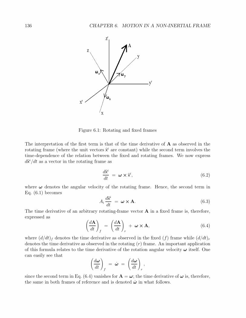
136 CHAPTER 6. MOTION IN A NON-INERTIAL FRAME
Figure 6.1: Rotating and fixed frames
The interpretation of the first term is that of the time derivative of A as observed in therotating frame (where the unit vectors xi are constant) while the second term involves thetime-dependence of the relation between the fixed and rotating frames. We now expressdxi/dt as a vector in the rotating frame as
dxi
dt= ω × xi, (6.2)
where ω denotes the angular velocity of the rotating frame. Hence, the second term inEq. (6.1) becomes
Aidxi
dt= ω ×A. (6.3)
The time derivative of an arbitrary rotating-frame vector A in a fixed frame is, therefore,expressed as (
dA
dt
)
f
=
(dA
dt
)
r
+ ω ×A, (6.4)
where (d/dt)f denotes the time derivative as observed in the fixed (f) frame while (d/dt)rdenotes the time derivative as observed in the rotating (r) frame. An important applicationof this formula relates to the time derivative of the rotation angular velocity ω itself. Onecan easily see that (
dω
dt
)
f
= ω =
(dω
dt
)
r
,
since the second term in Eq. (6.4) vanishes for A = ω; the time derivative of ω is, therefore,the same in both frames of reference and is denoted ω in what follows.
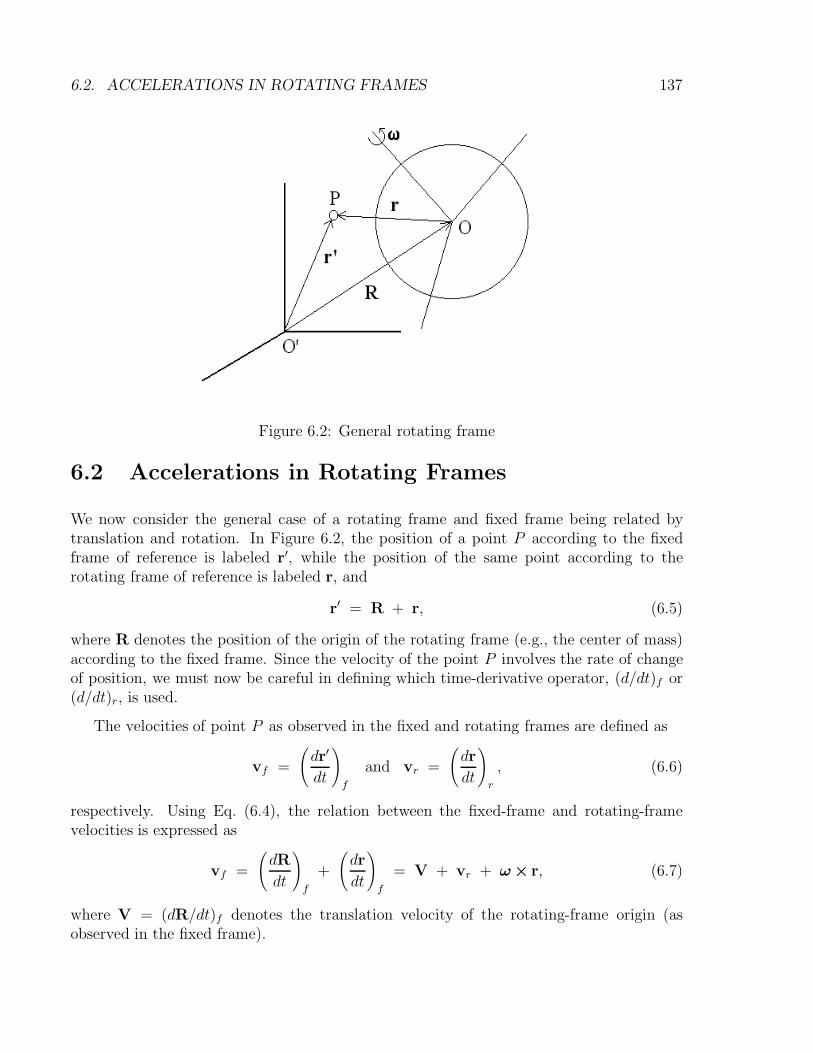
6.2. ACCELERATIONS IN ROTATING FRAMES 137
Figure 6.2: General rotating frame
6.2 Accelerations in Rotating Frames
We now consider the general case of a rotating frame and fixed frame being related bytranslation and rotation. In Figure 6.2, the position of a point P according to the fixedframe of reference is labeled r′, while the position of the same point according to therotating frame of reference is labeled r, and
r′ = R + r, (6.5)
where R denotes the position of the origin of the rotating frame (e.g., the center of mass)according to the fixed frame. Since the velocity of the point P involves the rate of changeof position, we must now be careful in defining which time-derivative operator, (d/dt)f or(d/dt)r, is used.
The velocities of point P as observed in the fixed and rotating frames are defined as
vf =
(dr′
dt
)
f
and vr =
(dr
dt
)
r
, (6.6)
respectively. Using Eq. (6.4), the relation between the fixed-frame and rotating-framevelocities is expressed as
vf =
(dR
dt
)
f
+
(dr
dt
)
f
= V + vr + ω × r, (6.7)
where V = (dR/dt)f denotes the translation velocity of the rotating-frame origin (asobserved in the fixed frame).
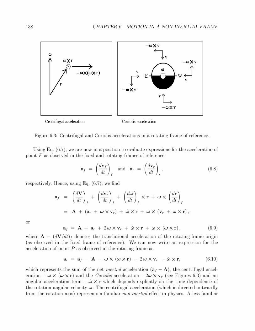
138 CHAPTER 6. MOTION IN A NON-INERTIAL FRAME
Figure 6.3: Centrifugal and Coriolis accelerations in a rotating frame of reference.
Using Eq. (6.7), we are now in a position to evaluate expressions for the acceleration ofpoint P as observed in the fixed and rotating frames of reference
af =
(dvfdt
)
f
and ar =
(dvrdt
)
r
, (6.8)
respectively. Hence, using Eq. (6.7), we find
af =
(dV
dt
)
f
+
(dvrdt
)
f
+
(dω
dt
)
f
× r + ω ×
(dr
dt
)
f
= A + (ar + ω ×vr) + ω × r + ω × (vr + ω × r) ,
oraf = A + ar + 2ω ×vr + ω × r + ω × (ω × r) , (6.9)
where A = (dV/dt)f denotes the translational acceleration of the rotating-frame origin(as observed in the fixed frame of reference). We can now write an expression for theacceleration of point P as observed in the rotating frame as
ar = af − A − ω × (ω × r) − 2ω ×vr − ω × r, (6.10)
which represents the sum of the net inertial acceleration (af − A), the centrifugal accel-eration −ω × (ω × r) and the Coriolis acceleration − 2ω ×vr (see Figures 6.3) and anangular acceleration term − ω × r which depends explicitly on the time dependence ofthe rotation angular velocity ω. The centrifugal acceleration (which is directed outwardlyfrom the rotation axis) represents a familiar non-inertial effect in physics. A less familiar
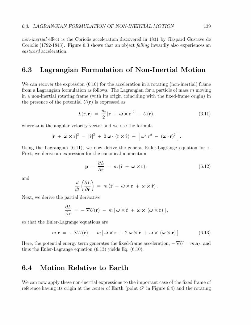
6.3. LAGRANGIAN FORMULATION OF NON-INERTIAL MOTION 139
non-inertial effect is the Coriolis acceleration discovered in 1831 by Gaspard Gustave deCoriolis (1792-1843). Figure 6.3 shows that an object falling inwardly also experiences aneastward acceleration.
6.3 Lagrangian Formulation of Non-Inertial Motion
We can recover the expression (6.10) for the acceleration in a rotating (non-inertial) framefrom a Lagrangian formulation as follows. The Lagrangian for a particle of mass m movingin a non-inertial rotating frame (with its origin coinciding with the fixed-frame origin) inthe presence of the potential U(r) is expressed as
L(r, r) =m
2|r + ω × r|2 − U(r), (6.11)
where ω is the angular velocity vector and we use the formula
|r + ω × r|2 = |r|2 + 2 ω · (r× r) +[ω2 r2 − (ω · r)2
].
Using the Lagrangian (6.11), we now derive the general Euler-Lagrange equation for r.First, we derive an expression for the canonical momentum
p =∂L
∂r= m (r + ω × r) , (6.12)
andd
dt
(∂L
∂r
)
= m (r + ω × r + ω × r) .
Next, we derive the partial derivative
∂L
∂r= − ∇U(r) − m [ ω × r + ω × (ω × r) ] ,
so that the Euler-Lagrange equations are
m r = − ∇U(r) − m [ ω × r + 2 ω × r + ω × (ω × r) ] . (6.13)
Here, the potential energy term generates the fixed-frame acceleration, −∇U = m af , andthus the Euler-Lagrange equation (6.13) yields Eq. (6.10).
6.4 Motion Relative to Earth
We can now apply these non-inertial expressions to the important case of the fixed frame ofreference having its origin at the center of Earth (point O′ in Figure 6.4) and the rotating
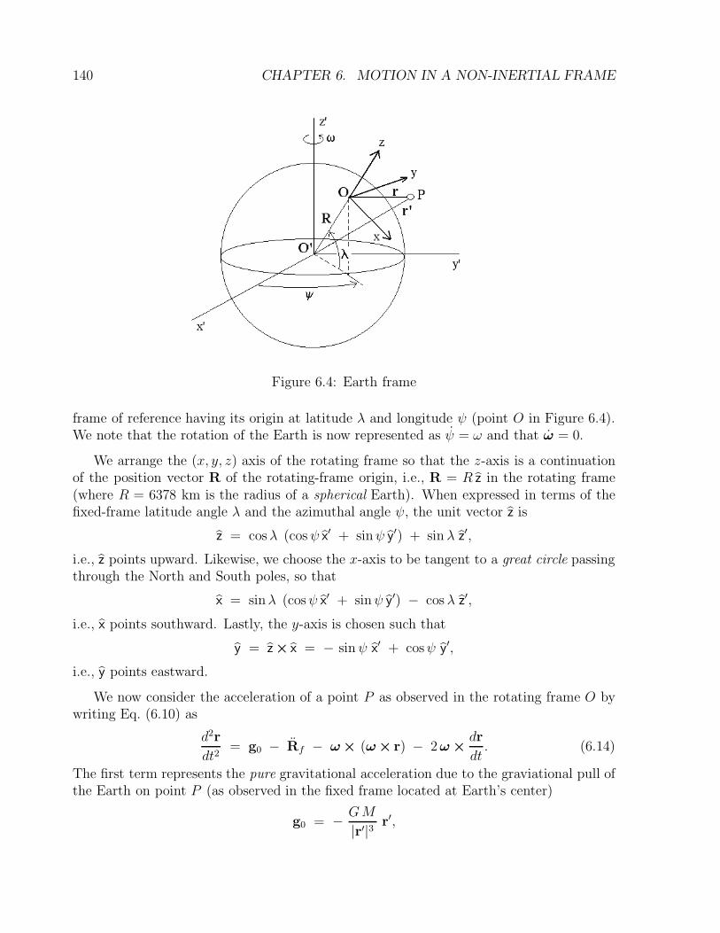
140 CHAPTER 6. MOTION IN A NON-INERTIAL FRAME
Figure 6.4: Earth frame
frame of reference having its origin at latitude λ and longitude ψ (point O in Figure 6.4).We note that the rotation of the Earth is now represented as ψ = ω and that ω = 0.
We arrange the (x, y, z) axis of the rotating frame so that the z-axis is a continuationof the position vector R of the rotating-frame origin, i.e., R = R z in the rotating frame(where R = 6378 km is the radius of a spherical Earth). When expressed in terms of thefixed-frame latitude angle λ and the azimuthal angle ψ, the unit vector z is
z = cosλ (cosψ x′ + sinψ y′) + sin λ z′,
i.e., z points upward. Likewise, we choose the x-axis to be tangent to a great circle passingthrough the North and South poles, so that
x = sinλ (cosψ x′ + sinψ y′) − cos λ z′,
i.e., x points southward. Lastly, the y-axis is chosen such that
y = z × x = − sinψ x′ + cosψ y′,
i.e., y points eastward.
We now consider the acceleration of a point P as observed in the rotating frame O bywriting Eq. (6.10) as
d2r
dt2= g0 − Rf − ω × (ω × r) − 2ω ×
dr
dt. (6.14)
The first term represents the pure gravitational acceleration due to the graviational pull ofthe Earth on point P (as observed in the fixed frame located at Earth’s center)
g0 = − GM
|r′|3 r′,
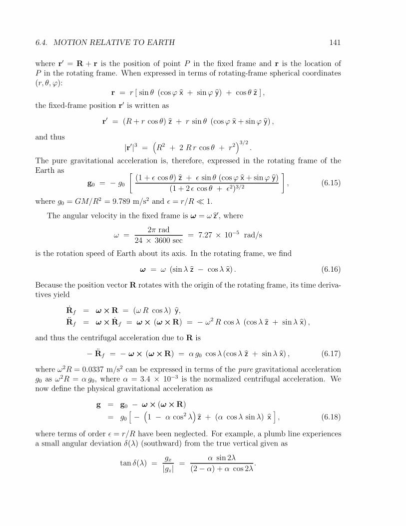
6.4. MOTION RELATIVE TO EARTH 141
where r′ = R + r is the position of point P in the fixed frame and r is the location ofP in the rotating frame. When expressed in terms of rotating-frame spherical coordinates(r, θ, ϕ):
r = r [ sin θ (cosϕ x + sinϕ y) + cos θ z ] ,
the fixed-frame position r′ is written as
r′ = (R+ r cos θ) z + r sin θ (cosϕ x + sinϕ y) ,
and thus
|r′|3 =(R2 + 2 R r cos θ + r2
)3/2.
The pure gravitational acceleration is, therefore, expressed in the rotating frame of theEarth as
g0 = − g0
[(1 + ε cos θ) z + ε sin θ (cosϕ x + sinϕ y)
(1 + 2 ε cos θ + ε2)3/2
]
, (6.15)
where g0 = GM/R2 = 9.789 m/s2 and ε = r/R 1.
The angular velocity in the fixed frame is ω = ω z′, where
ω =2π rad
24 × 3600 sec= 7.27 × 10⁻⁵ rad/s
is the rotation speed of Earth about its axis. In the rotating frame, we find
ω = ω (sinλ z − cosλ x) . (6.16)
Because the position vector R rotates with the origin of the rotating frame, its time deriva-tives yield
Rf = ω ×R = (ωR cosλ) y,
Rf = ω × Rf = ω × (ω ×R) = − ω2R cos λ (cos λ z + sinλ x) ,
and thus the centrifugal acceleration due to R is
− Rf = − ω × (ω ×R) = αg0 cos λ (cosλ z + sinλ x) , (6.17)
where ω2R = 0.0337 m/s2 can be expressed in terms of the pure gravitational accelerationg0 as ω2R = αg0, where α = 3.4 × 10⁻³ is the normalized centrifugal acceleration. Wenow define the physical gravitational acceleration as
g = g0 − ω × (ω ×R)
= g0
[−(1 − α cos2 λ
)z + (α cosλ sin λ) x
], (6.18)
where terms of order ε = r/R have been neglected. For example, a plumb line experiencesa small angular deviation δ(λ) (southward) from the true vertical given as
tan δ(λ) =gx|gz|
=α sin 2λ
(2 − α) + α cos 2λ.
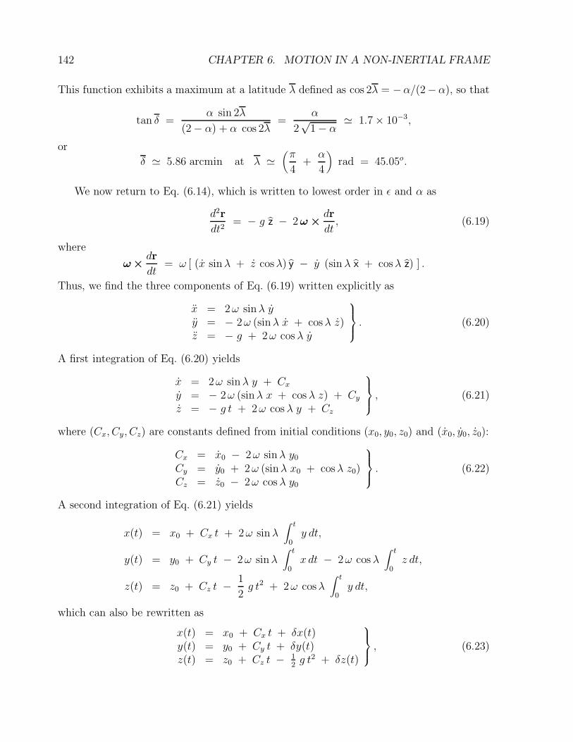
142 CHAPTER 6. MOTION IN A NON-INERTIAL FRAME
This function exhibits a maximum at a latitude λ defined as cos 2λ = −α/(2−α), so that
tan δ =α sin 2λ
(2 − α) + α cos 2λ=
α
2√
1 − α' 1.7 × 10⁻³,
or
δ ' 5.86 arcmin at λ '(π
4+
α
4
)rad = 45.05o.
We now return to Eq. (6.14), which is written to lowest order in ε and α as
d2r
dt2= − g z − 2ω ×
dr
dt, (6.19)
where
ω ×dr
dt= ω [ (x sinλ + z cosλ) y − y (sin λ x + cosλ z) ] .
Thus, we find the three components of Eq. (6.19) written explicitly as
x = 2ω sinλ yy = − 2ω (sinλ x + cosλ z)z = − g + 2ω cos λ y
. (6.20)
A first integration of Eq. (6.20) yields
x = 2ω sinλ y + Cxy = − 2ω (sinλ x + cos λ z) + Cyz = − g t + 2ω cos λ y + Cz
, (6.21)
where (Cx, Cy, Cz) are constants defined from initial conditions (x0, y0, z0) and (x0, y0, z0):
Cx = x0 − 2ω sinλ y0
Cy = y0 + 2ω (sinλ x0 + cosλ z0)Cz = z0 − 2ω cos λ y0
. (6.22)
A second integration of Eq. (6.21) yields
x(t) = x0 + Cx t + 2ω sinλ∫ t
0y dt,
y(t) = y0 + Cy t − 2ω sinλ∫ t
0x dt − 2ω cos λ
∫ t
0z dt,
z(t) = z0 + Cz t − 1
2g t2 + 2ω cosλ
∫ t
0y dt,
which can also be rewritten as
x(t) = x0 + Cx t + δx(t)y(t) = y0 + Cy t + δy(t)z(t) = z0 + Cz t − 1
2g t2 + δz(t)
, (6.23)

6.4. MOTION RELATIVE TO EARTH 143
where the Coriolis drifts are
δx(t) = 2ω sinλ(y0 t +
1
2Cy t
2 +∫ t
0δy dt
)(6.24)
δy(t) = − 2ω sinλ(x0 t +
1
2Cx t
2 +∫ t
0δx dt
)
− 2ω cos λ(z0 t +
1
2Cz t
2 − 1
6g t3 +
∫ t
0δz dt
)(6.25)
δz(t) = 2ω cosλ(y0 t +
1
2Cy t
2 +∫ t
0δy dt
). (6.26)
Note that each Coriolis drift can be expressed as an infinite series in powers of ω and thatall Coriolis effects vanish when ω = 0.
6.4.1 Free-Fall Problem Revisited
As an example of the importance of Coriolis effects in describing motion relative to Earth,we consider the simple free-fall problem, where
(x0, y0, z0) = (0, 0, h) and (x0, y0, z0) = (0, 0, 0),
so that the constants (6.22) are
Cx = 0 = Cz and Cy = 2ω h cos λ.
Substituting these constants into Eqs. (6.23) and keeping only terms up to first order in ω,we find
x(t) = 0, (6.27)
y(t) =1
3gt3 ω cos λ, (6.28)
z(t) = h − 1
2gt2. (6.29)
Hence, a free-falling object starting from rest touches the ground z(T ) = 0 after a time
T =√
2h/g after which time the object has drifted eastward by a distance of
y(T ) =1
3gT 3 ω cos λ =
ω cos λ
3
√8h3
g,
which is maximum at the equator. At a height of 100 m and latitude 45o, for example, wefind an eastward drift of 1.55 cm.
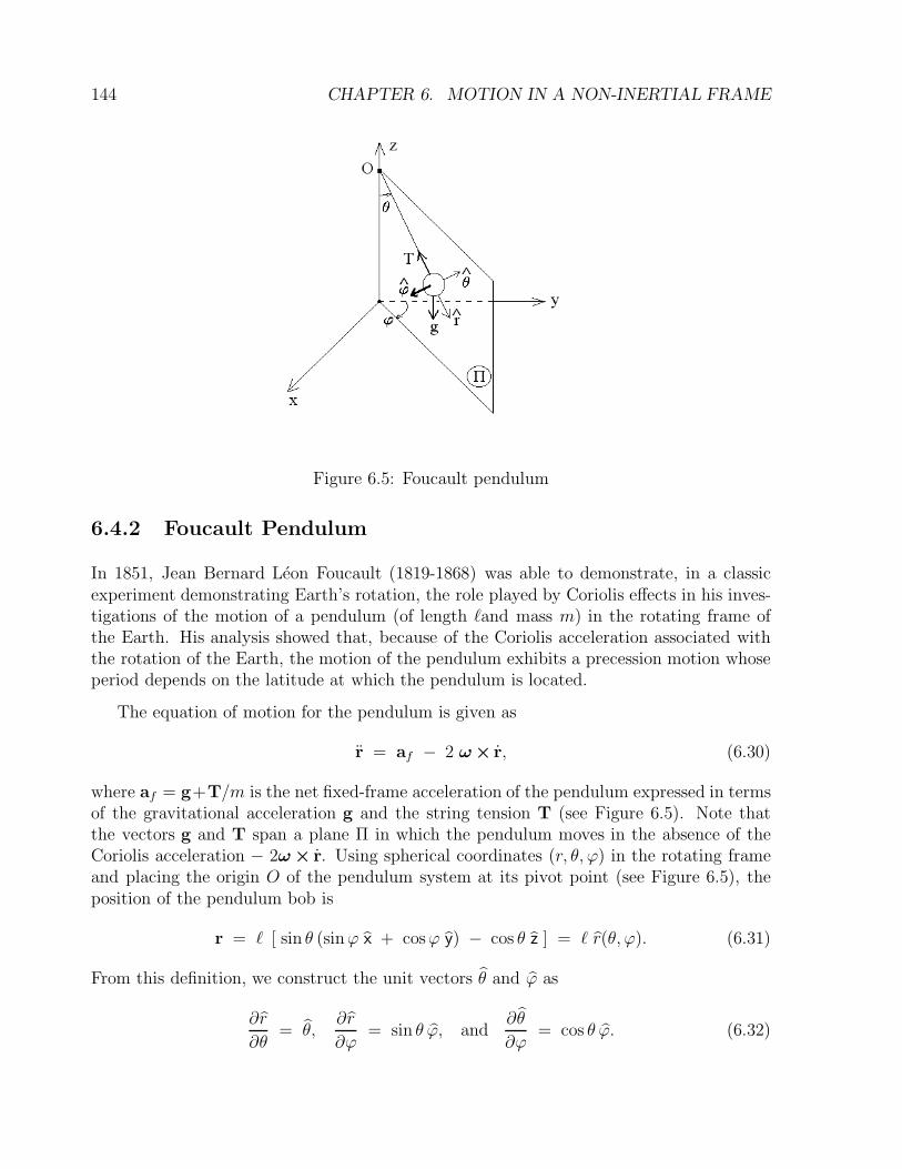
144 CHAPTER 6. MOTION IN A NON-INERTIAL FRAME
Figure 6.5: Foucault pendulum
6.4.2 Foucault Pendulum
In 1851, Jean Bernard Leon Foucault (1819-1868) was able to demonstrate, in a classicexperiment demonstrating Earth’s rotation, the role played by Coriolis effects in his inves-tigations of the motion of a pendulum (of length `and mass m) in the rotating frame ofthe Earth. His analysis showed that, because of the Coriolis acceleration associated withthe rotation of the Earth, the motion of the pendulum exhibits a precession motion whoseperiod depends on the latitude at which the pendulum is located.
The equation of motion for the pendulum is given as
r = af − 2 ω × r, (6.30)
where af = g+T/m is the net fixed-frame acceleration of the pendulum expressed in termsof the gravitational acceleration g and the string tension T (see Figure 6.5). Note thatthe vectors g and T span a plane Π in which the pendulum moves in the absence of theCoriolis acceleration − 2ω × r. Using spherical coordinates (r, θ, ϕ) in the rotating frameand placing the origin O of the pendulum system at its pivot point (see Figure 6.5), theposition of the pendulum bob is
r = ` [ sin θ (sinϕ x + cosϕ y) − cos θ z ] = ` r(θ, ϕ). (6.31)
From this definition, we construct the unit vectors θ and ϕ as
∂r
∂θ= θ,
∂r
∂ϕ= sin θ ϕ, and
∂θ
∂ϕ= cos θ ϕ. (6.32)
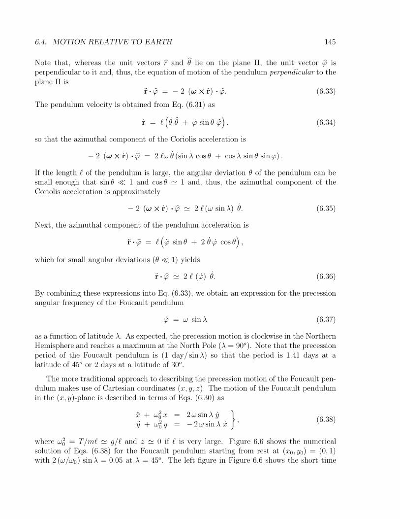
6.4. MOTION RELATIVE TO EARTH 145
Note that, whereas the unit vectors r and θ lie on the plane Π, the unit vector ϕ isperpendicular to it and, thus, the equation of motion of the pendulum perpendicular to theplane Π is
r · ϕ = − 2 (ω × r) · ϕ. (6.33)
The pendulum velocity is obtained from Eq. (6.31) as
r = `(θ θ + ϕ sin θ ϕ
), (6.34)
so that the azimuthal component of the Coriolis acceleration is
− 2 (ω × r) · ϕ = 2 `ω θ (sinλ cos θ + cosλ sin θ sinϕ) .
If the length ` of the pendulum is large, the angular deviation θ of the pendulum can besmall enough that sin θ 1 and cos θ ' 1 and, thus, the azimuthal component of theCoriolis acceleration is approximately
− 2 (ω × r) · ϕ ' 2 ` (ω sin λ) θ. (6.35)
Next, the azimuthal component of the pendulum acceleration is
r · ϕ = `(ϕ sin θ + 2 θ ϕ cos θ
),
which for small angular deviations (θ 1) yields
r · ϕ ' 2 ` (ϕ) θ. (6.36)
By combining these expressions into Eq. (6.33), we obtain an expression for the precessionangular frequency of the Foucault pendulum
ϕ = ω sin λ (6.37)
as a function of latitude λ. As expected, the precession motion is clockwise in the NorthernHemisphere and reaches a maximum at the North Pole (λ = 90o). Note that the precessionperiod of the Foucault pendulum is (1 day/ sinλ) so that the period is 1.41 days at alatitude of 45o or 2 days at a latitude of 30o.
The more traditional approach to describing the precession motion of the Foucault pen-dulum makes use of Cartesian coordinates (x, y, z). The motion of the Foucault pendulumin the (x, y)-plane is described in terms of Eqs. (6.30) as
x + ω20 x = 2ω sinλ y
y + ω20 y = − 2ω sinλ x
, (6.38)
where ω20 = T/m` ' g/` and z ' 0 if ` is very large. Figure 6.6 shows the numerical
solution of Eqs. (6.38) for the Foucault pendulum starting from rest at (x0, y0) = (0, 1)with 2 (ω/ω0) sinλ = 0.05 at λ = 45o. The left figure in Figure 6.6 shows the short time
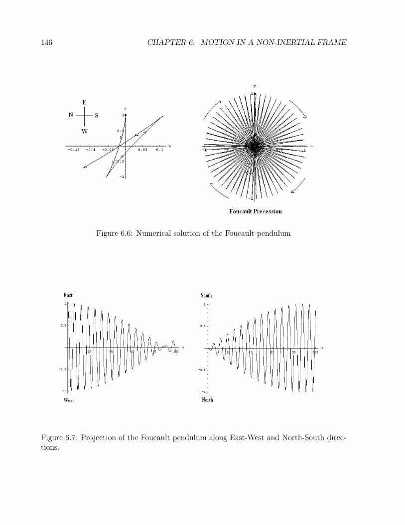
146 CHAPTER 6. MOTION IN A NON-INERTIAL FRAME
Figure 6.6: Numerical solution of the Foucault pendulum
Figure 6.7: Projection of the Foucault pendulum along East-West and North-South direc-tions.
6.4. MOTION RELATIVE TO EARTH 147
behavior (note the different x and y scales) while the right figure in Figure 6.6 shows thecomplete Foucault precession. Figure 6.7 shows that, over a finite period of time, thependulum motion progressively moves from the East-West axis to the North-South axis.We now define the complex-valued function
q = y + i x = ` sin θ eiϕ, (6.39)
so that Eq. (6.38) becomes
q + ω20 q − 2i ω sinλ q = 0.
Next, we insert the eigenfunction q(t) = ρ exp(iΩt) into this equation and find that thesolution for the eigenfrequency Ω is
Ω = ω sinλ ±√ω2 sin2 λ + ω2
0,
so that the eigenfunction is
q = ρ eiω sinλ t sin(√
ω2 sin2 λ + ω20 t).
By comparing this solution with Eq. (6.39), we finally find
ρ sin(√
ω2 sin2 λ + ω20 t)
= ` sin θ ' ` θ(t),
andϕ(t) = (ω sinλ) t,
from which we recover the Foucault pendulum precession frequency (6.37).
148 CHAPTER 6. MOTION IN A NON-INERTIAL FRAME
6.5 Problems
Problem 1
(a) Consider the case involving motion on the (x, y)-plane perpendicular to the angularvelocity vector ω = ω z with the potential energy
U(r) =1
2k(x2 + y2
).
Using the Euler-Lagrange equations (6.13), derive the equations of motion for x and y.
(b) By using the equations of motion derived in Part (a), show that the canonical angularmomentum ` = z · (r×p) is a constant of the motion.
Problem 2
If a particle is projected vertically upward to a height h above a point on the Earth’ssurface at a northern latitude λ, show that it strikes the ground at a point
4ω
3cos λ
√8h3
g
to the west. (Neglect air resistance, and consider only small vertical heights.)
Problem 3
For the potentialU(r, r) = V (r) + σ · r× r,
where V (r) denotes an arbitrary central potential and σ denotes an arbitrary constantvector, derive the Euler-Lagrange equations of motion in terms of spherical coordinates.
Problem 4
The Lagrangian for the Foucault-pendulum equations (6.38) is
L(x, y; x, y) =1
2
(x2 + y2
)− ω2
0
2
(x2 + y2
)+ ω sin λ (x y − x y) .
(a) By using the polar transformation x(t) = ρ(t) cosϕ(t) and y(t) = ρ(t) sinϕ(t), derivethe new Lagrangian L(ρ; ρ, ϕ).
(b) Since the new Lagrangian L(ρ; ρ, ϕ) is independent of ϕ, derive an expression for theconserved momentum pϕ and find the Routhian R(ρ, ρ; pϕ) and the Routh-Euler-Lagrangianequation for ρ.
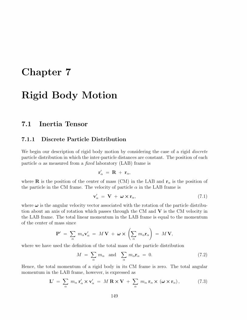
Chapter 7
Rigid Body Motion
7.1 Inertia Tensor
7.1.1 Discrete Particle Distribution
We begin our description of rigid body motion by considering the case of a rigid discreteparticle distribution in which the inter-particle distances are constant. The position of eachparticle α as measured from a fixed laboratory (LAB) frame is
r′α = R + rα,
where R is the position of the center of mass (CM) in the LAB and rα is the position ofthe particle in the CM frame. The velocity of particle α in the LAB frame is
v′α = V + ω × rα, (7.1)
where ω is the angular velocity vector associated with the rotation of the particle distribu-tion about an axis of rotation which passes through the CM and V is the CM velocity inthe LAB frame. The total linear momentum in the LAB frame is equal to the momentumof the center of mass since
P′ =∑
α
mαv′α = M V + ω ×
(∑
α
mαrα
)
= M V,
where we have used the definition of the total mass of the particle distribution
M =∑
α
mα and∑
α
mαrα = 0. (7.2)
Hence, the total momentum of a rigid body in its CM frame is zero. The total angularmomentum in the LAB frame, however, is expressed as
L′ =∑
α
mα r′α ×v′α = M R×V +
∑
α
mα rα × (ω × rα) , (7.3)
149
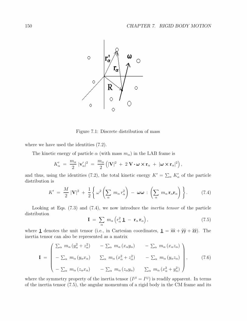
150 CHAPTER 7. RIGID BODY MOTION
Figure 7.1: Discrete distribution of mass
where we have used the identities (7.2).
The kinetic energy of particle α (with mass mα) in the LAB frame is
K ′α =
mα
2|v′α|2 =
mα
2
(|V|2 + 2 V · ω × rα + |ω × rα|2
),
and thus, using the identities (7.2), the total kinetic energy K ′ =∑α K
′α of the particle
distribution is
K ′ =M
2|V|2 +
1
2
ω2
(∑
α
mα r2α
)
− ωω :
(∑
α
mα rαrα
)
. (7.4)
Looking at Eqs. (7.3) and (7.4), we now introduce the inertia tensor of the particledistribution
I =∑
α
mα
(r2α 1 − rα rα
), (7.5)
where 1 denotes the unit tensor (i.e., in Cartesian coordinates, 1 = xx + yy + zz). Theinertia tensor can also be represented as a matrix
I =
∑α mα (y2
α + z2α) − ∑
α mα (xαyα) − ∑α mα (xαzα)
− ∑α mα (yαxα)
∑α mα (x2
α + z2α) − ∑
α mα (yαzα)
− ∑α mα (zαxα) − ∑
α mα (zαyα)∑α mα (x2
α + y2α)
, (7.6)
where the symmetry property of the inertia tensor (I ji = I ij) is readily apparent. In termsof the inertia tensor (7.5), the angular momentum of a rigid body in the CM frame and its
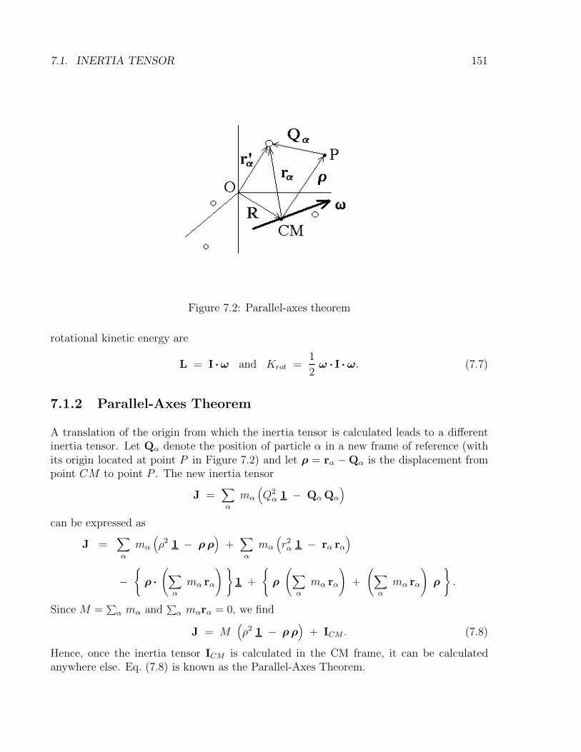
7.1. INERTIA TENSOR 151
Figure 7.2: Parallel-axes theorem
rotational kinetic energy are
L = I ·ω and Krot =1
2ω · I · ω. (7.7)
7.1.2 Parallel-Axes Theorem
A translation of the origin from which the inertia tensor is calculated leads to a differentinertia tensor. Let Qα denote the position of particle α in a new frame of reference (withits origin located at point P in Figure 7.2) and let ρ = rα − Qα is the displacement frompoint CM to point P . The new inertia tensor
J =∑
α
mα
(Q2α 1 − QαQα
)
can be expressed as
J =∑
α
mα
(ρ2 1 − ρ ρ
)+∑
α
mα
(r2α 1 − rα rα
)
−
ρ ·
(∑
α
mα rα
)
1 +
ρ
(∑
α
mα rα
)
+
(∑
α
mα rα
)
ρ
.
Since M =∑α mα and
∑α mαrα = 0, we find
J = M(ρ2 1 − ρ ρ
)+ ICM . (7.8)
Hence, once the inertia tensor ICM is calculated in the CM frame, it can be calculatedanywhere else. Eq. (7.8) is known as the Parallel-Axes Theorem.
152 CHAPTER 7. RIGID BODY MOTION
Figure 7.3: Continuous distribution of mass
7.1.3 Continuous Particle Distribution
For a continuous particle distribution the inertia tensor (7.5) becomes
I =∫dm
(r2 1 − rr
), (7.9)
where dm(r) = ρ(r) d3r is the infinitesimal mass element at point r, with mass densityρ(r).
Consider, for example, the case of a uniform cube of mass M and volume b3, withdm = (M/b3) dx dy dz. The inertia tensor (7.9) in the LAB frame (with the origin placedat one of its corners) has the components
J11 =M
b3
∫ b
0dx
∫ b
0dy
∫ b
0dz ·
(y2 + z2
)=
2
3M b2 = J22 = J33 (7.10)
J12 = − M
b3
∫ b
0dx
∫ b
0dy
∫ b
0dz · x y = − 1
4M b2 = J23 = J31 (7.11)
and thus the inertia matrix for the cube is
J =M b2
12
8 − 3 − 3
− 3 8 − 3
− 3 − 3 8
. (7.12)

7.1. INERTIA TENSOR 153
Figure 7.4: Cube
On the other hand, the inertia tensor calculated in the CM frame has the components
I11 =M
b3
∫ b/2
− b/2dx
∫ b/2
− b/2dy
∫ b/2
− b/2dz ·
(y2 + z2
)=
1
6M b2 = I22 = I33(7.13)
I12 = − M
b3
∫ b/2
− b/2dx
∫ b/2
− b/2dy
∫ b/2
− b/2dz · x y = 0 = I23 = I31 (7.14)
and thus the CM inertia matrix for the cube is
I =M b2
6
1 0 0
0 1 0
0 0 1
. (7.15)
The displacement vector ρ from the CM point to the corner O is given as
ρ = − b
2(x + y + z) ,
so that ρ2 = 3b2/4. By using the Parallel-Axis Theorem (7.8), the inertia tensor
M(ρ2 1 − ρ ρ
)=
M b2
4
2 −1 −1
−1 2 −1
−1 −1 2
when added to the CM inertia tensor (7.15), yields the inertia tensor (7.12)
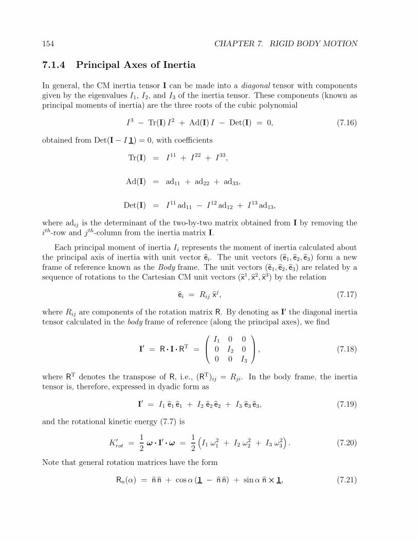
154 CHAPTER 7. RIGID BODY MOTION
7.1.4 Principal Axes of Inertia
In general, the CM inertia tensor I can be made into a diagonal tensor with componentsgiven by the eigenvalues I1, I2, and I3 of the inertia tensor. These components (known asprincipal moments of inertia) are the three roots of the cubic polynomial
I3 − Tr(I) I2 + Ad(I) I − Det(I) = 0, (7.16)
obtained from Det(I − I 1) = 0, with coefficients
Tr(I) = I11 + I22 + I33,
Ad(I) = ad11 + ad22 + ad33,
Det(I) = I11 ad11 − I12 ad12 + I13 ad13,
where adij is the determinant of the two-by-two matrix obtained from I by removing theith-row and jth-column from the inertia matrix I.
Each principal moment of inertia Ii represents the moment of inertia calculated aboutthe principal axis of inertia with unit vector ei. The unit vectors (e1, e2, e3) form a newframe of reference known as the Body frame. The unit vectors (e1, e2, e3) are related by asequence of rotations to the Cartesian CM unit vectors (x1, x2, x3) by the relation
ei = Rij xj, (7.17)
where Rij are components of the rotation matrix R. By denoting as I′ the diagonal inertiatensor calculated in the body frame of reference (along the principal axes), we find
I′ = R · I ·RT =
I1 0 00 I2 00 0 I3
, (7.18)
where RT denotes the transpose of R, i.e., (RT)ij = Rji. In the body frame, the inertiatensor is, therefore, expressed in dyadic form as
I′ = I1 e1 e1 + I2 e2 e2 + I3 e3 e3, (7.19)
and the rotational kinetic energy (7.7) is
K ′rot =
1
2ω · I′ · ω =
1
2
(I1 ω
21 + I2 ω
22 + I3 ω
23
). (7.20)
Note that general rotation matrices have the form
Rn(α) = n n + cosα (1 − n n) + sinα n × 1, (7.21)

7.1. INERTIA TENSOR 155
Figure 7.5: Dumbbell
where the unit vector n defines the axis of rotation about which an angular rotation ofangle α is performed according to the right-hand-rule.
A rigid body can be classified into one of three different categories. First, a rigidbody can be said to be a spherical top if its three principal moments of inertia are equal(I1 = I2 = I3), i.e., the three roots of the cubic polynomial (7.16) are triply degenerate.Next, a rigid body can be said to be a symmetric top if two of its principal moments ofinertia are equal (I1 = I2 6= I3), i.e., I3 is a single root and I1 = I2 are doubly-degenerateroots of the cubic polynomial (7.16). Lastly, when the three roots (I1 6= I2 6= I3) are allsingle roots of the cubic polynomial (7.16), a rigid body is said to be an asymmetric top.
Before proceeding further, we consider the example of a dumbbell composed of twoequal point masses m placed at the ends of a massless rod of total length 2 b and rotatingabout the z-axis with angular frequency ω. Here, the positions of the two masses areexpressed as
r± = ± b [sin θ (cosϕ x + sinϕ y) + cos θ z ] ,
so that the CM inertia tensor is
I = 2mb2
1 − cos2 ϕ sin2 θ − cosϕ sinϕ sin2 θ − cosϕ cos θ sin θ
− cosϕ sinϕ sin2 θ 1 − sin2 ϕ sin2 θ − sinϕ cos θ sin θ
− cosϕ cos θ sin θ − sinϕ cos θ sin θ 1 − cos2 θ
. (7.22)
After some tedious algebra, we find Tr(I) = 4mb2, Ad(I) = (2mb2)2, and Det(I) = 0,and thus the cubic polynomial (7.16) has the single root I3 = 0 and the double rootI1 = I2 = 2mb2, which makes the dumbbell a symmetric top.
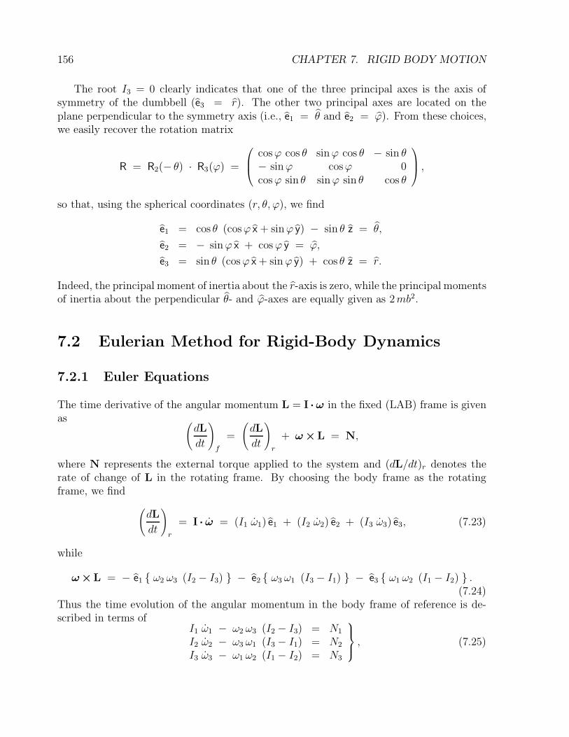
156 CHAPTER 7. RIGID BODY MOTION
The root I3 = 0 clearly indicates that one of the three principal axes is the axis ofsymmetry of the dumbbell (e3 = r). The other two principal axes are located on theplane perpendicular to the symmetry axis (i.e., e1 = θ and e2 = ϕ). From these choices,we easily recover the rotation matrix
R = R2(− θ) · R3(ϕ) =
cosϕ cos θ sinϕ cos θ − sin θ− sinϕ cosϕ 0cosϕ sin θ sinϕ sin θ cos θ
,
so that, using the spherical coordinates (r, θ, ϕ), we find
e1 = cos θ (cosϕ x + sinϕ y) − sin θ z = θ,
e2 = − sinϕ x + cosϕ y = ϕ,
e3 = sin θ (cosϕ x + sinϕ y) + cos θ z = r.
Indeed, the principal moment of inertia about the r-axis is zero, while the principal momentsof inertia about the perpendicular θ- and ϕ-axes are equally given as 2mb2.
7.2 Eulerian Method for Rigid-Body Dynamics
7.2.1 Euler Equations
The time derivative of the angular momentum L = I · ω in the fixed (LAB) frame is givenas (
dL
dt
)
f
=
(dL
dt
)
r
+ ω ×L = N,
where N represents the external torque applied to the system and (dL/dt)r denotes therate of change of L in the rotating frame. By choosing the body frame as the rotatingframe, we find
(dL
dt
)
r
= I · ω = (I1 ω1) e1 + (I2 ω2) e2 + (I3 ω3) e3, (7.23)
while
ω ×L = − e1 ω2 ω3 (I2 − I3) − e2 ω3 ω1 (I3 − I1) − e3 ω1 ω2 (I1 − I2) .(7.24)
Thus the time evolution of the angular momentum in the body frame of reference is de-scribed in terms of
I1 ω1 − ω2 ω3 (I2 − I3) = N1
I2 ω2 − ω3 ω1 (I3 − I1) = N2
I3 ω3 − ω1 ω2 (I1 − I2) = N3
, (7.25)
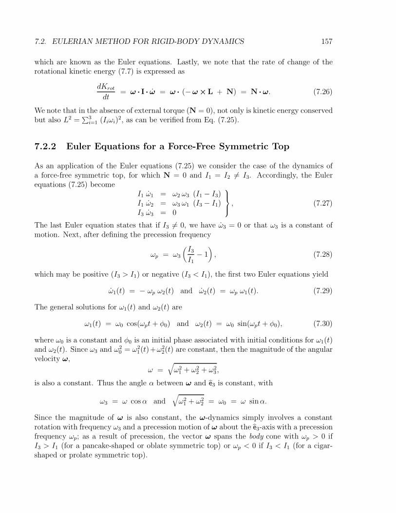
7.2. EULERIAN METHOD FOR RIGID-BODY DYNAMICS 157
which are known as the Euler equations. Lastly, we note that the rate of change of therotational kinetic energy (7.7) is expressed as
dKrot
dt= ω · I · ω = ω · (−ω ×L + N) = N · ω. (7.26)
We note that in the absence of external torque (N = 0), not only is kinetic energy conservedbut also L2 =
∑3i=1 (Iiωi)
2, as can be verified from Eq. (7.25).
7.2.2 Euler Equations for a Force-Free Symmetric Top
As an application of the Euler equations (7.25) we consider the case of the dynamics ofa force-free symmetric top, for which N = 0 and I1 = I2 6= I3. Accordingly, the Eulerequations (7.25) become
I1 ω1 = ω2 ω3 (I1 − I3)I1 ω2 = ω3 ω1 (I3 − I1)I3 ω3 = 0
, (7.27)
The last Euler equation states that if I3 6= 0, we have ω3 = 0 or that ω3 is a constant ofmotion. Next, after defining the precession frequency
ωp = ω3
(I3I1
− 1), (7.28)
which may be positive (I3 > I1) or negative (I3 < I1), the first two Euler equations yield
ω1(t) = − ωp ω2(t) and ω2(t) = ωp ω1(t). (7.29)
The general solutions for ω1(t) and ω2(t) are
ω1(t) = ω0 cos(ωpt+ φ0) and ω2(t) = ω0 sin(ωpt+ φ0), (7.30)
where ω0 is a constant and φ0 is an initial phase associated with initial conditions for ω1(t)and ω2(t). Since ω3 and ω2
0 = ω21(t)+ω2
2(t) are constant, then the magnitude of the angularvelocity ω,
ω =√ω2
1 + ω22 + ω2
3 ,
is also a constant. Thus the angle α between ω and e3 is constant, with
ω3 = ω cosα and√ω2
1 + ω22 = ω0 = ω sinα.
Since the magnitude of ω is also constant, the ω-dynamics simply involves a constantrotation with frequency ω3 and a precession motion of ω about the e3-axis with a precessionfrequency ωp; as a result of precession, the vector ω spans the body cone with ωp > 0 ifI3 > I1 (for a pancake-shaped or oblate symmetric top) or ωp < 0 if I3 < I1 (for a cigar-shaped or prolate symmetric top).
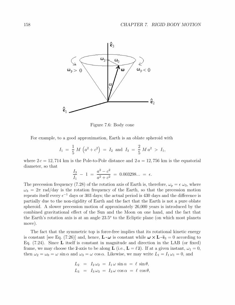
158 CHAPTER 7. RIGID BODY MOTION
Figure 7.6: Body cone
For example, to a good approximation, Earth is an oblate spheroid with
I1 =1
5M
(a2 + c2
)= I2 and I3 =
2
5M a2 > I1,
where 2 c = 12, 714 km is the Pole-to-Pole distance and 2a = 12, 756 km is the equatorialdiameter, so that
I3I1
− 1 =a2 − c2
a2 + c2= 0.003298... = ε.
The precession frequency (7.28) of the rotation axis of Earth is, therefore, ωp = ε ω3, whereω3 = 2π rad/day is the rotation frequency of the Earth, so that the precession motionrepeats itself every ε−1 days or 303 days; the actual period is 430 days and the difference ispartially due to the non-rigidity of Earth and the fact that the Earth is not a pure oblatespheroid. A slower precession motion of approximately 26,000 years is introduced by thecombined gravitational effect of the Sun and the Moon on one hand, and the fact thatthe Earth’s rotation axis is at an angle 23.5o to the Ecliptic plane (on which most planetsmove).
The fact that the symmetric top is force-free implies that its rotational kinetic energyis constant [see Eq. (7.26)] and, hence, L ·ω is constant while ω ×L · e3 = 0 according toEq. (7.24). Since L itself is constant in magnitude and direction in the LAB (or fixed)frame, we may choose the z-axis to be along L (i.e., L = ` z). If at a given instant, ω1 = 0,then ω2 = ω0 = ω sinα and ω3 = ω cosα. Likewise, we may write L1 = I1 ω1 = 0, and
L2 = I2 ω2 = I1 ω sinα = ` sin θ,
L3 = I3 ω3 = I3 ω cosα = ` cos θ,

7.2. EULERIAN METHOD FOR RIGID-BODY DYNAMICS 159
where L ·ω = `ω cos θ, with θ represents the space-cone angle. From these equations, wefind the relation between the body-cone angle α and the space-cone angle θ to be
tan θ =(I1I3
)tanα, (7.31)
which shows that θ > α for I3 < I1 and θ < α for I3 > I1.
7.2.3 Euler Equations for a Force-Free Asymmetric Top
We now consider the general case of an asymmetric top moving under force-free conditions.To facilitate our discussion, we assume that I1 > I2 > I3 and thus Euler’s equations (7.25)for a force-free asymmetric top are
I1 ω1 = ω2 ω3 (I2 − I3)I2 ω2 = − ω3 ω1 (I1 − I3)I3 ω3 = ω1 ω2 (I1 − I2)
. (7.32)
As previously mentioned, the Euler equations (7.32) have two constants of the motion:kinetic energy
K =1
2
(I1 ω
21 + I2 ω
22 + I3 ω
23
), (7.33)
and the squared magnitude of the angular momentum
L2 = I21 ω
21 + I2
2 ω22 + I3
3 ω23. (7.34)
Figure 7.7 shows the numerical solution of the Euler equations (7.32) subject to theinitial condition (ω10, ω20, ω30) = (2, 0, 1) for different values of the ratios I1/I3 and I2/I3.Note that in the limit I1 = I2 (corresponding to a symmetric top), the top evolves solelyon the (ω1, ω2)-plane at constant ω3. As I1 increases from I2, the asymmetric top exhibitsdoubly-periodic behavior in the full (ω1, ω2, ω3)-space until the motion becomes restricted tothe (ω2, ω3)-plane in the limit I1 I2. One also clearly notes the existence of a separatrixwhich appears as I1 reaches the critical value
I1c =I22
+
√I22
4+ I3 (I2 − I3)
(ω30
ω10
)2
,
at constant I2 and I3 and given initial conditions (ω10, ω20, ω30).
We note that the existence of two constants of the motion, Eqs. (7.33) and (7.34), forthe three Euler equations (7.32) means that we may express the Euler equations in termsof a single equation. For this purpose, we introduce the constants
σ = 2 I1K − L2 and ρ = L2 − 2 I3K,
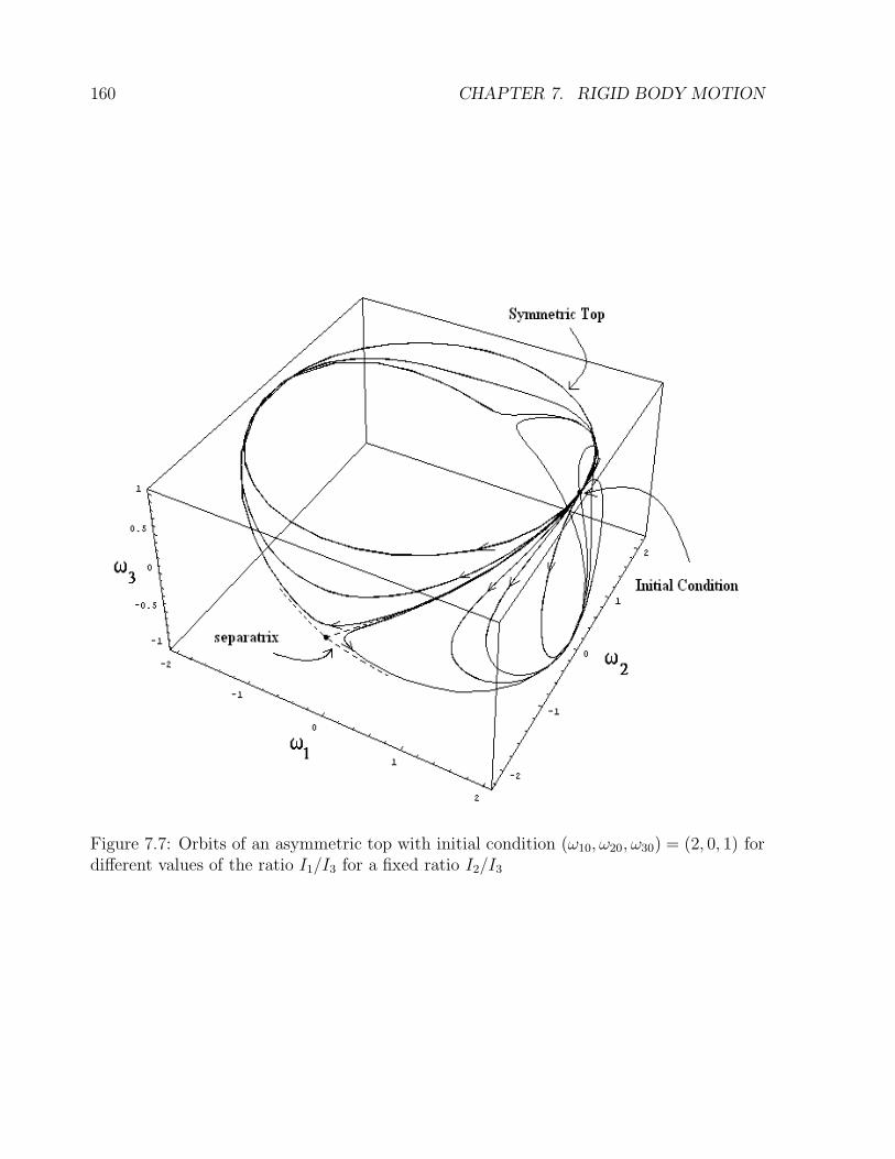
160 CHAPTER 7. RIGID BODY MOTION
Figure 7.7: Orbits of an asymmetric top with initial condition (ω10, ω20, ω30) = (2, 0, 1) fordifferent values of the ratio I1/I3 for a fixed ratio I2/I3
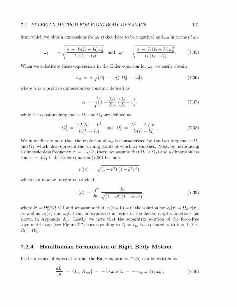
7.2. EULERIAN METHOD FOR RIGID-BODY DYNAMICS 161
from which we obtain expressions for ω1 (taken here to be negative) and ω3 in terms of ω2:
ω1 = −√√√√ρ − I2(I2 − I3)ω2
2
I1 (I1 − I3)and ω3 =
√√√√σ − I2(I1 − I2)ω22
I3 (I1 − I3). (7.35)
When we substitute these expressions in the Euler equation for ω2, we easily obtain
ω2 = α√
(Ω21 − ω2
2) (Ω23 − ω2
2), (7.36)
where α is a positive dimensionless constant defined as
α =
√(1 − I2
I1
) (I2I3
− 1), (7.37)
while the constant frequencies Ω1 and Ω3 are defined as
Ω21 =
2 I1K − L2
I2(I1 − I2)and Ω2
3 =L2 − 2 I3K
I2(I2 − I3). (7.38)
We immediately note that the evolution of ω2 is characterized by the two frequencies Ω1
and Ω3, which also represent the turning points at which ω2 vanishes. Next, by introducinga dimensionless frequency ν = ω2/Ω3 (here, we assume that Ω1 ≥ Ω3) and a dimensionlesstime τ = αΩ1 t, the Euler equation (7.36) becomes
ν ′(τ ) =√
(1 − ν2) (1 − k2 ν2),
which can now be integrated to yield
τ (ν) =∫ ν
0
ds√
(1 − s2) (1 − k2 s2), (7.39)
where k2 = Ω23/Ω
21 ≤ 1 and we assume that ω2(t = 0) = 0; the solution for ω2(τ ) = Ω3 ν(τ ),
as well as ω1(τ ) and ω3(τ ) can be expressed in terms of the Jacobi elliptic functions (asshown in Appendix A). Lastly, we note that the separatrix solution of the force-freeasymmetric top (see Figure 7.7) corresponding to I1 = I1c is associated with k = 1 (i.e.,Ω1 = Ω3).
7.2.4 Hamiltonian Formulation of Rigid Body Motion
In the absence of external torque, the Euler equations (7.25) can be written as
dLidt
= Li, Krot = − i · ω ×L = − εijk ωj (Ik ωk), (7.40)
162 CHAPTER 7. RIGID BODY MOTION
Figure 7.8: Euler angles
where the Poisson bracket , is defined in terms of two arbitrary functions F (L) andG(L) as
F, G = − L ·∂F
∂L×∂G
∂L. (7.41)
Note that, for a general function F (L) of angular momentum and in the absence of externaltorque, we find
dF
dt= − L ·
∂F
∂L×∂Krot
∂L= − ∂F
∂L· ω ×L,
and thus any function of |L| is a constant of the motion for rigid body dynamics.
7.3 Lagrangian Method for Rigid-Body Dynamics
7.3.1 Eulerian Angles as generalized Lagrangian Coordinates
To describe the physical state of a rotating object with principal moments of inertia(I1, I2, I3), we need the three Eulerian angles (ϕ, θ, ψ) in the body frame of reference (seeFigure 7.8). The Eulerian angle ϕ is associated with the rotation of the fixed-frame unitvectors (x, y, z) about the z-axis. We thus obtain the new unit vectors (x′, y′, z′) defined as
x′
y′
z′
=
= R3(ϕ)︷ ︸︸ ︷
cosϕ sinϕ 0
− sinϕ cosϕ 00 0 1
·
x
y
z
(7.42)
The rotation matrix R3(ϕ) has the following properties associated with a general rotationmatrix Rn(α), defined in Eq. (7.21), where a rotation of axes about the xn-axis is performedthrough an arbitrary angle α. First, the matrix Rn(−α) is the inverse matrix of Rn(α), i.e.,
Rn(−α) · Rn(α) = 1 = Rn(α) · Rn(−α).
7.3. LAGRANGIAN METHOD FOR RIGID-BODY DYNAMICS 163
Next, the determinant of Rn(α) is + 1 and the eigenvalues of Rn(α) are +1, eiα, and e− iα
(see Appendix A.2 for further details).
The Eulerian angle θ is associated with the rotation of the unit vectors (x′, y′, z′) aboutthe x′-axis. We thus obtain the new unit vectors (x′′, y′′, z′′) defined as
x′′
y′′
z′′
=
= R1(θ)︷ ︸︸ ︷
1 0 00 cos θ sin θ0 − sin θ cos θ
·
x′
y′
z′
(7.43)
The Eulerian angle ψ is associated with the rotation of the unit vectors (x′′, y′′, z′′) aboutthe z′′-axis. We thus obtain the body-frame unit vectors (e1, e2, e3) defined as
e1
e2
e3
=
= R3(ψ)︷ ︸︸ ︷
cosψ sinψ 0
− sinψ cosψ 00 0 1
·
x′′
y′′
z′′
(7.44)
Hence, the relation between the fixed-frame unit vectors (x, y, z) and the body-frameunit vectors (e1, e2, e3) involves the matrix R = R3(ψ) · R1(θ) · R3(ϕ), such that ei = Rij xj ,or
e1 = cosψ ⊥ + sinψ (cos θ ϕ+ sin θ z)
e2 = − sinψ ⊥ + cosψ (cos θ ϕ+ sin θ z)
e3 = − sin θ ϕ + cos θ z
, (7.45)
where ϕ = − sinϕ x + cosϕ y and ⊥ = cosϕ x + sinϕ y = ϕ× z.
7.3.2 Angular Velocity in terms of Eulerian Angles
The angular velocity ω represented in the three Figures above is expressed as
ω = ϕ z + θ x′ + ψ e3.
The unit vectors z and x′ are written in terms of the body-frame unit vectors (e1, e2, e3) as
z = sin θ (sinψ e1 + cosψ e2) + cos θ e3,
x′ = x′′ = cosψ e1 − sinψ e2.
The angular velocity can, therefore, be written exclusively in the body frame of referencein terms of the Euler basis vectors (7.45) as
ω = ω1 e1 + ω2 e2 + ω3 e3, (7.46)
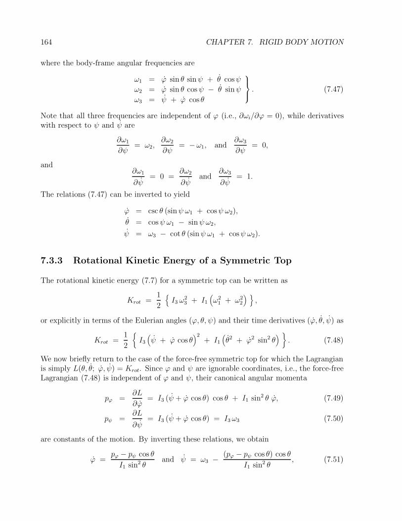
164 CHAPTER 7. RIGID BODY MOTION
where the body-frame angular frequencies are
ω1 = ϕ sin θ sinψ + θ cosψ
ω2 = ϕ sin θ cosψ − θ sinψ
ω3 = ψ + ϕ cos θ
. (7.47)
Note that all three frequencies are independent of ϕ (i.e., ∂ωi/∂ϕ = 0), while derivativeswith respect to ψ and ψ are
∂ω1
∂ψ= ω2,
∂ω2
∂ψ= −ω1, and
∂ω3
∂ψ= 0,
and∂ω1
∂ψ= 0 =
∂ω2
∂ψand
∂ω3
∂ψ= 1.
The relations (7.47) can be inverted to yield
ϕ = csc θ (sinψ ω1 + cosψ ω2),
θ = cosψ ω1 − sinψ ω2,
ψ = ω3 − cot θ (sinψ ω1 + cosψ ω2).
7.3.3 Rotational Kinetic Energy of a Symmetric Top
The rotational kinetic energy (7.7) for a symmetric top can be written as
Krot =1
2
I3 ω
23 + I1
(ω2
1 + ω22
) ,
or explicitly in terms of the Eulerian angles (ϕ, θ, ψ) and their time derivatives (ϕ, θ, ψ) as
Krot =1
2
I3(ψ + ϕ cos θ
)2+ I1
(θ2 + ϕ2 sin2 θ
) . (7.48)
We now briefly return to the case of the force-free symmetric top for which the Lagrangianis simply L(θ, θ; ϕ, ψ) = Krot. Since ϕ and ψ are ignorable coordinates, i.e., the force-freeLagrangian (7.48) is independent of ϕ and ψ, their canonical angular momenta
pϕ =∂L
∂ϕ= I3 (ψ + ϕ cos θ) cos θ + I1 sin2 θ ϕ, (7.49)
pψ =∂L
∂ψ= I3 (ψ + ϕ cos θ) = I3 ω3 (7.50)
are constants of the motion. By inverting these relations, we obtain
ϕ =pϕ − pψ cos θ
I1 sin2 θand ψ = ω3 − (pϕ − pψ cos θ) cos θ
I1 sin2 θ, (7.51)
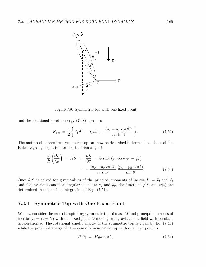
7.3. LAGRANGIAN METHOD FOR RIGID-BODY DYNAMICS 165
Figure 7.9: Symmetric top with one fixed point
and the rotational kinetic energy (7.48) becomes
Krot =1
2
I1 θ2 + I3 ω
23 +
(pϕ − pψ cos θ)2
I1 sin2 θ
. (7.52)
The motion of a force-free symmetric top can now be described in terms of solutions of theEuler-Lagrange equation for the Eulerian angle θ:
d
dt
(∂L
∂θ
)
= I1 θ =∂L
∂θ= ϕ sin θ (I1 cos θ ϕ − pψ)
= − (pϕ − pψ cos θ)
I1 sin θ
(pψ − pϕ cos θ)
sin2 θ. (7.53)
Once θ(t) is solved for given values of the principal moments of inertia I1 = I2 and I3and the invariant canonical angular momenta pϕ and pψ, the functions ϕ(t) and ψ(t) aredetermined from the time integration of Eqs. (7.51).
7.3.4 Symmetric Top with One Fixed Point
We now consider the case of a spinning symmetric top of mass M and principal moments ofinertia (I1 = I2 6= I3) with one fixed point O moving in a gravitational field with constantacceleration g. The rotational kinetic energy of the symmetric top is given by Eq. (7.48)while the potential energy for the case of a symmetric top with one fixed point is
U(θ) = Mgh cos θ, (7.54)
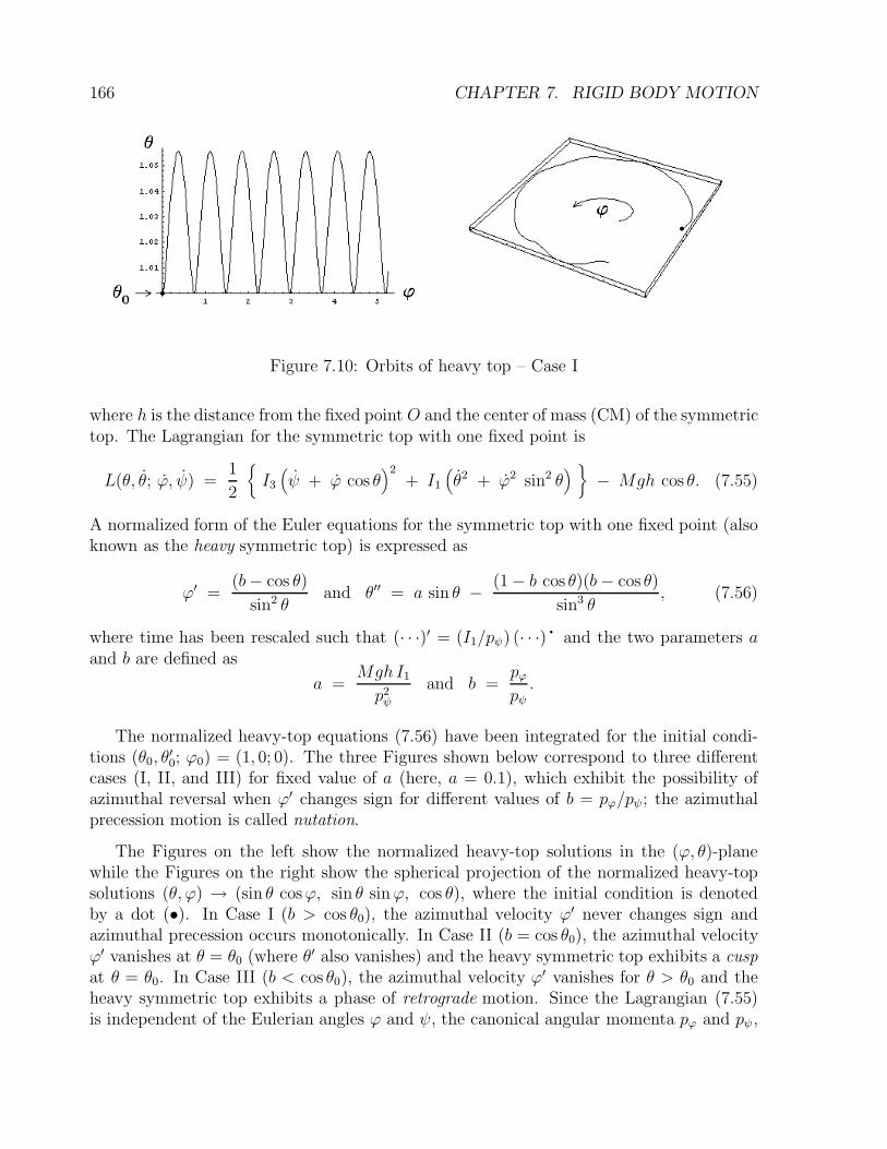
166 CHAPTER 7. RIGID BODY MOTION
Figure 7.10: Orbits of heavy top – Case I
where h is the distance from the fixed point O and the center of mass (CM) of the symmetrictop. The Lagrangian for the symmetric top with one fixed point is
L(θ, θ; ϕ, ψ) =1
2
I3(ψ + ϕ cos θ
)2+ I1
(θ2 + ϕ2 sin2 θ
) − Mgh cos θ. (7.55)
A normalized form of the Euler equations for the symmetric top with one fixed point (alsoknown as the heavy symmetric top) is expressed as
ϕ′ =(b− cos θ)
sin2 θand θ′′ = a sin θ − (1 − b cos θ)(b− cos θ)
sin3 θ, (7.56)
where time has been rescaled such that (· · ·)′ = (I1/pψ) (· · ·) · and the two parameters aand b are defined as
a =MghI1p2ψ
and b =pϕpψ.
The normalized heavy-top equations (7.56) have been integrated for the initial condi-tions (θ0, θ
′0; ϕ0) = (1, 0; 0). The three Figures shown below correspond to three different
cases (I, II, and III) for fixed value of a (here, a = 0.1), which exhibit the possibility ofazimuthal reversal when ϕ′ changes sign for different values of b = pϕ/pψ; the azimuthalprecession motion is called nutation.
The Figures on the left show the normalized heavy-top solutions in the (ϕ, θ)-planewhile the Figures on the right show the spherical projection of the normalized heavy-topsolutions (θ, ϕ) → (sin θ cosϕ, sin θ sinϕ, cos θ), where the initial condition is denotedby a dot (•). In Case I (b > cos θ0), the azimuthal velocity ϕ′ never changes sign andazimuthal precession occurs monotonically. In Case II (b = cos θ0), the azimuthal velocityϕ′ vanishes at θ = θ0 (where θ′ also vanishes) and the heavy symmetric top exhibits a cuspat θ = θ0. In Case III (b < cos θ0), the azimuthal velocity ϕ′ vanishes for θ > θ0 and theheavy symmetric top exhibits a phase of retrograde motion. Since the Lagrangian (7.55)is independent of the Eulerian angles ϕ and ψ, the canonical angular momenta pϕ and pψ,
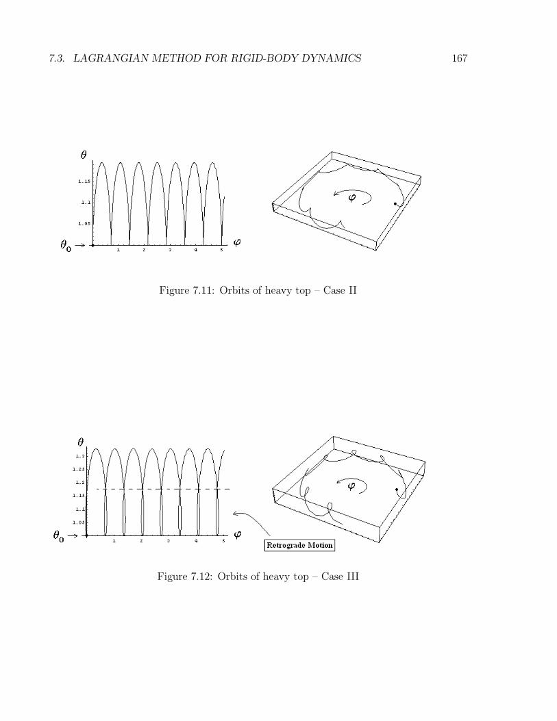
7.3. LAGRANGIAN METHOD FOR RIGID-BODY DYNAMICS 167
Figure 7.11: Orbits of heavy top – Case II
Figure 7.12: Orbits of heavy top – Case III
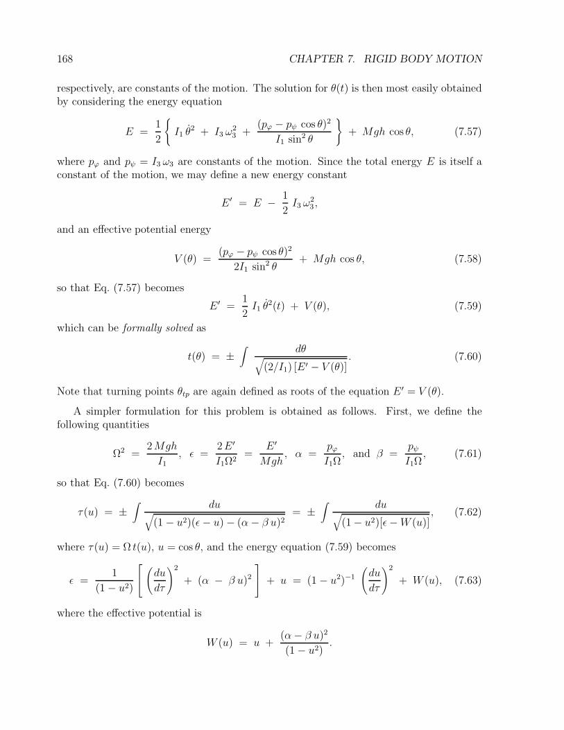
168 CHAPTER 7. RIGID BODY MOTION
respectively, are constants of the motion. The solution for θ(t) is then most easily obtainedby considering the energy equation
E =1
2
I1 θ2 + I3 ω
23 +
(pϕ − pψ cos θ)2
I1 sin2 θ
+ Mgh cos θ, (7.57)
where pϕ and pψ = I3 ω3 are constants of the motion. Since the total energy E is itself aconstant of the motion, we may define a new energy constant
E ′ = E − 1
2I3 ω
23 ,
and an effective potential energy
V (θ) =(pϕ − pψ cos θ)2
2I1 sin2 θ+ Mgh cos θ, (7.58)
so that Eq. (7.57) becomes
E ′ =1
2I1 θ
2(t) + V (θ), (7.59)
which can be formally solved as
t(θ) = ±∫
dθ√
(2/I1) [E ′ − V (θ)]. (7.60)
Note that turning points θtp are again defined as roots of the equation E ′ = V (θ).
A simpler formulation for this problem is obtained as follows. First, we define thefollowing quantities
Ω2 =2Mgh
I1, ε =
2E ′
I1Ω2=
E ′
Mgh, α =
pϕI1Ω
, and β =pψI1Ω
, (7.61)
so that Eq. (7.60) becomes
τ (u) = ±∫ du√
(1 − u2)(ε− u) − (α − β u)2= ±
∫ du√
(1 − u2)[ε−W (u)], (7.62)
where τ (u) = Ω t(u), u = cos θ, and the energy equation (7.59) becomes
ε =1
(1 − u2)
(du
dτ
)2
+ (α − β u)2
+ u = (1 − u2)−1
(du
dτ
)2
+ W (u), (7.63)
where the effective potential is
W (u) = u +(α− β u)2
(1 − u2).
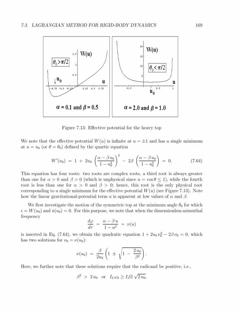
7.3. LAGRANGIAN METHOD FOR RIGID-BODY DYNAMICS 169
Figure 7.13: Effective potential for the heavy top
We note that the effective potential W (u) is infinite at u = ±1 and has a single minimumat u = u0 (or θ = θ0) defined by the quartic equation
W ′(u0) = 1 + 2u0
(α − β u0
1 − u20
)2
− 2β
(α − β u0
1 − u20
)
= 0. (7.64)
This equation has four roots: two roots are complex roots, a third root is always greaterthan one for α > 0 and β > 0 (which is unphysical since u = cos θ ≤ 1), while the fourthroot is less than one for α > 0 and β > 0; hence, this root is the only physical rootcorresponding to a single minimum for the effective potential W (u) (see Figure 7.13). Notehow the linear gravitational-potential term u is apparent at low values of α and β.
We first investigate the motion of the symmetric top at the minimum angle θ0 for whichε = W (u0) and u(u0) = 0. For this purpose, we note that when the dimensionless azimuthalfrequency
dϕ
dτ=
α− β u
1 − u2= ν(u)
is inserted in Eq. (7.64), we obtain the quadratic equation 1 + 2u0 ν20 − 2β ν0 = 0, which
has two solutions for ν0 = ν(u0):
ν(u0) =β
2u0
(
1 ±√
1 − 2u0
β2
)
.
Here, we further note that these solutions require that the radicand be positive, i.e.,
β2 > 2u0 or I3 ω3 ≥ I1Ω√
2u0,
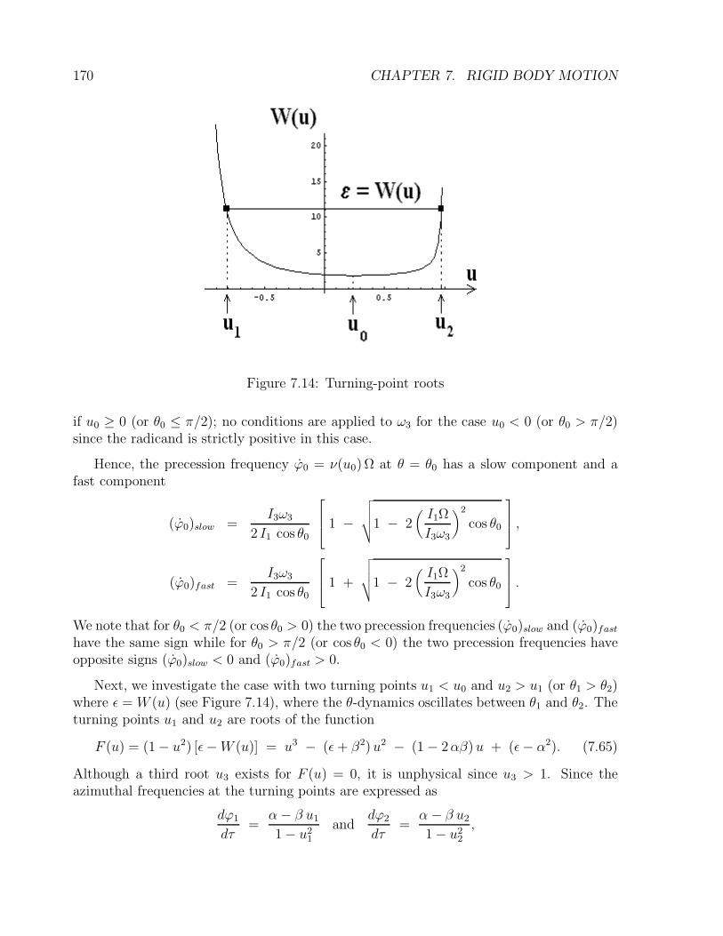
170 CHAPTER 7. RIGID BODY MOTION
Figure 7.14: Turning-point roots
if u0 ≥ 0 (or θ0 ≤ π/2); no conditions are applied to ω3 for the case u0 < 0 (or θ0 > π/2)since the radicand is strictly positive in this case.
Hence, the precession frequency ϕ0 = ν(u0)Ω at θ = θ0 has a slow component and afast component
(ϕ0)slow =I3ω3
2 I1 cos θ0
1 −
√√√√1 − 2(I1Ω
I3ω3
)2
cos θ0
,
(ϕ0)fast =I3ω3
2 I1 cos θ0
1 +
√√√√1 − 2(I1Ω
I3ω3
)2
cos θ0
.
We note that for θ0 < π/2 (or cos θ0 > 0) the two precession frequencies (ϕ0)slow and (ϕ0)fasthave the same sign while for θ0 > π/2 (or cos θ0 < 0) the two precession frequencies haveopposite signs (ϕ0)slow < 0 and (ϕ0)fast > 0.
Next, we investigate the case with two turning points u1 < u0 and u2 > u1 (or θ1 > θ2)where ε = W (u) (see Figure 7.14), where the θ-dynamics oscillates between θ1 and θ2. Theturning points u1 and u2 are roots of the function
F (u) = (1 − u2) [ε−W (u)] = u3 − (ε+ β2)u2 − (1 − 2αβ)u + (ε− α2). (7.65)
Although a third root u3 exists for F (u) = 0, it is unphysical since u3 > 1. Since theazimuthal frequencies at the turning points are expressed as
dϕ1
dτ=
α− β u1
1 − u21
anddϕ2
dτ=
α − β u2
1 − u22
,
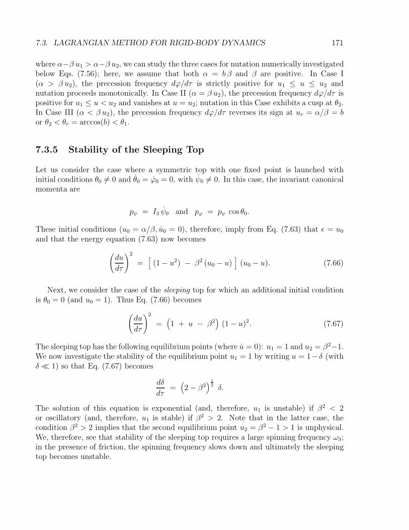
7.3. LAGRANGIAN METHOD FOR RIGID-BODY DYNAMICS 171
where α−β u1 > α−β u2, we can study the three cases for nutation numerically investigatedbelow Eqs. (7.56); here, we assume that both α = b β and β are positive. In Case I(α > β u2), the precession frequency dϕ/dτ is strictly positive for u1 ≤ u ≤ u2 andnutation proceeds monotonically. In Case II (α = β u2), the precession frequency dϕ/dτ ispositive for u1 ≤ u < u2 and vanishes at u = u2; nutation in this Case exhibits a cusp at θ2.In Case III (α < β u2), the precession frequency dϕ/dτ reverses its sign at ur = α/β = bor θ2 < θr = arccos(b) < θ1.
7.3.5 Stability of the Sleeping Top
Let us consider the case where a symmetric top with one fixed point is launched withinitial conditions θ0 6= 0 and θ0 = ϕ0 = 0, with ψ0 6= 0. In this case, the invariant canonicalmomenta are
pψ = I3 ψ0 and pϕ = pψ cos θ0.
These initial conditions (u0 = α/β, u0 = 0), therefore, imply from Eq. (7.63) that ε = u0
and that the energy equation (7.63) now becomes
(du
dτ
)2
=[
(1 − u2) − β2 (u0 − u)]
(u0 − u). (7.66)
Next, we consider the case of the sleeping top for which an additional initial conditionis θ0 = 0 (and u0 = 1). Thus Eq. (7.66) becomes
(du
dτ
)2
=(1 + u − β2
)(1 − u)2. (7.67)
The sleeping top has the following equilibrium points (where u = 0): u1 = 1 and u2 = β2−1.We now investigate the stability of the equilibrium point u1 = 1 by writing u = 1− δ (withδ 1) so that Eq. (7.67) becomes
dδ
dτ=(2 − β2
) 1
2 δ.
The solution of this equation is exponential (and, therefore, u1 is unstable) if β2 < 2or oscillatory (and, therefore, u1 is stable) if β2 > 2. Note that in the latter case, thecondition β2 > 2 implies that the second equilibrium point u2 = β2 − 1 > 1 is unphysical.We, therefore, see that stability of the sleeping top requires a large spinning frequency ω3;in the presence of friction, the spinning frequency slows down and ultimately the sleepingtop becomes unstable.

172 CHAPTER 7. RIGID BODY MOTION
7.4 Problems
Problem 1
Consider a thin homogeneous rectangular plate of mass M and area ab that lies on the(x, y)-plane.
(a) Show that the inertia tensor (calculated in the reference frame with its origin at pointO in the Figure above) takes the form
I =
A −C 0−C B 00 0 A +B
,
and find suitable expressions for A, B, and C in terms of M , a, and b.
(b) Show that by performing a rotation of the coordinate axes about the z-axis through anangle θ, the new inertia tensor is
I′(θ) = R(θ) · I · RT (θ) =
A′ −C ′ 0
−C ′ B ′ 00 0 A′ +B ′
,
where
A′ = A cos2 θ + B sin2 θ − C sin 2θ
B ′ = A sin2 θ + B cos2 θ + C sin 2θ
C ′ = C cos 2θ − 1
2(B − A) sin 2θ.
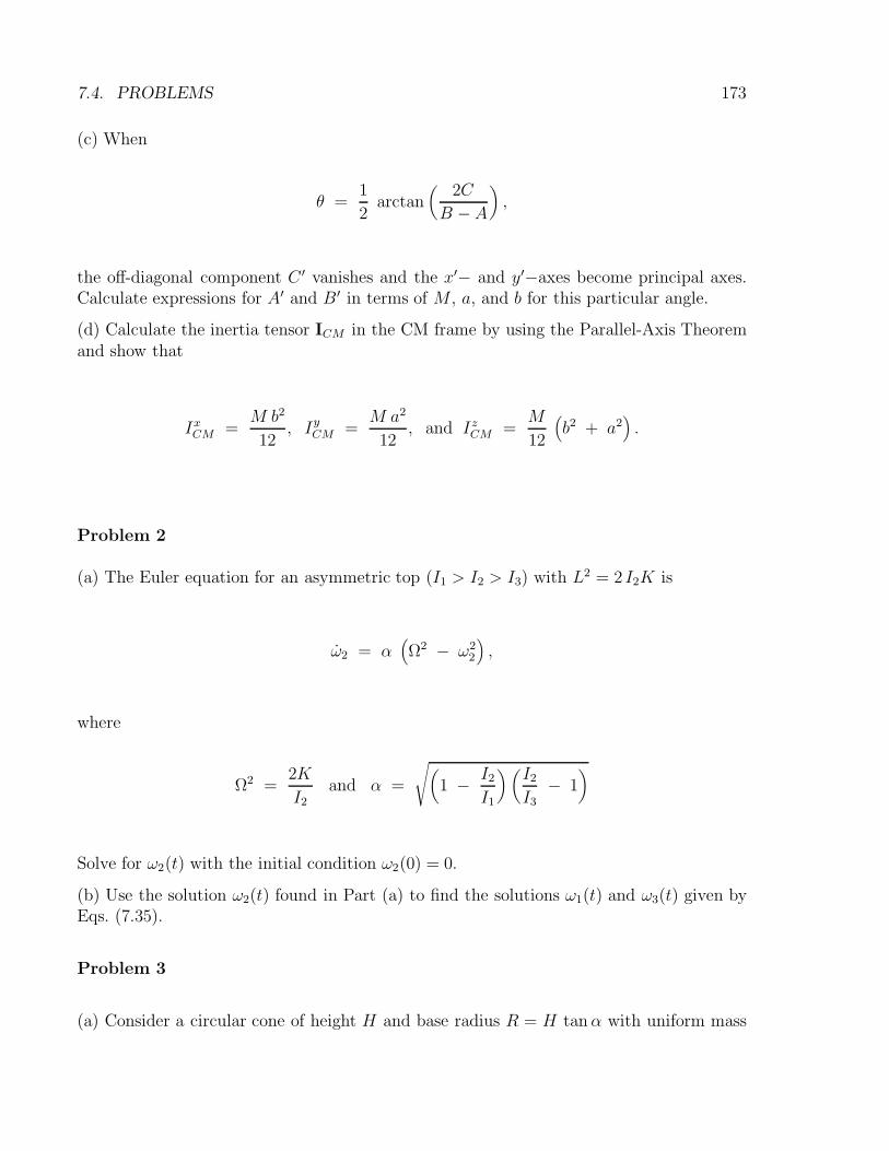
7.4. PROBLEMS 173
(c) When
θ =1
2arctan
(2C
B − A
),
the off-diagonal component C ′ vanishes and the x′− and y′−axes become principal axes.Calculate expressions for A′ and B ′ in terms of M , a, and b for this particular angle.
(d) Calculate the inertia tensor ICM in the CM frame by using the Parallel-Axis Theoremand show that
IxCM =M b2
12, IyCM =
M a2
12, and IzCM =
M
12
(b2 + a2
).
Problem 2
(a) The Euler equation for an asymmetric top (I1 > I2 > I3) with L2 = 2 I2K is
ω2 = α(Ω2 − ω2
2
),
where
Ω2 =2K
I2and α =
√(1 − I2
I1
)(I2I3
− 1)
Solve for ω2(t) with the initial condition ω2(0) = 0.
(b) Use the solution ω2(t) found in Part (a) to find the solutions ω1(t) and ω3(t) given byEqs. (7.35).
Problem 3
(a) Consider a circular cone of height H and base radius R = H tanα with uniform mass
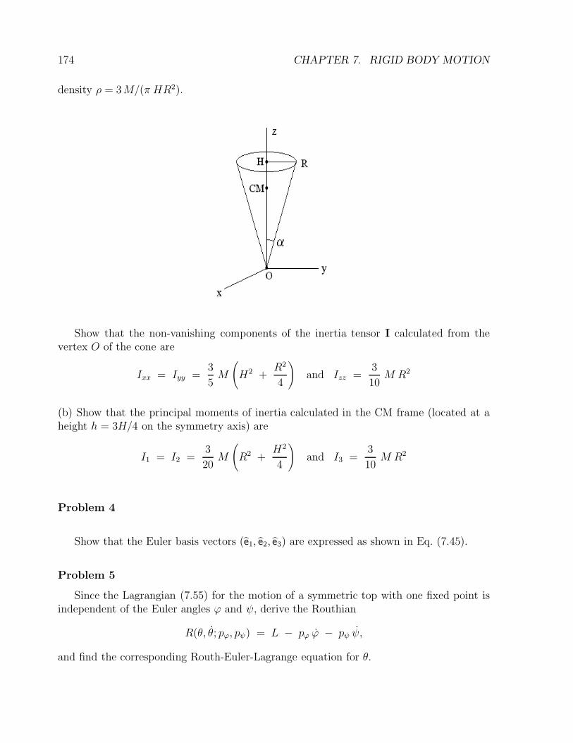
174 CHAPTER 7. RIGID BODY MOTION
density ρ = 3M/(π HR2).
Show that the non-vanishing components of the inertia tensor I calculated from thevertex O of the cone are
Ixx = Iyy =3
5M
(
H2 +R2
4
)
and Izz =3
10M R2
(b) Show that the principal moments of inertia calculated in the CM frame (located at aheight h = 3H/4 on the symmetry axis) are
I1 = I2 =3
20M
(
R2 +H2
4
)
and I3 =3
10M R2
Problem 4
Show that the Euler basis vectors (e1, e2, e3) are expressed as shown in Eq. (7.45).
Problem 5
Since the Lagrangian (7.55) for the motion of a symmetric top with one fixed point isindependent of the Euler angles ϕ and ψ, derive the Routhian
R(θ, θ; pϕ, pψ) = L − pϕ ϕ − pψ ψ,
and find the corresponding Routh-Euler-Lagrange equation for θ.
Chapter 8
Normal-Mode Analysis
8.1 Stability of Equilibrium Points
A nonlinear force equation mx = f(x) has equilibrium points (labeled x0) when f(x0)vanishes. The stability of the equilibrium point x0 is determined by the sign of f ′(x0): theequilibrium point x0 is stable if f ′(x0) < 0 or it is unstable if f ′(x0) > 0. Since f(x) is alsoderived from a potential V (x) as f(x) = −V ′(x), we say that the equilibrium point x0 isstable (or unstable) if V ′′(x0) is positive (or negative).
8.1.1 Bead on a Rotating Hoop
In Chap. 2, we considered the problem of a bead of mass m sliding freely on a hoop ofradius r rotating with angular velocity ω0 in a constant gravitational field with accelerationg. The Lagrangian for this system is
L(θ, θ) =m
2r2θ2 +
(m
2r2ω2
0 sin2 θ + mgr cos θ)
=m
2r2θ2 − V (θ),
where V (θ) denotes the effective potential, and the Euler-Lagrange equation for θ is
mr2 θ = −V ′(θ) = − mr2ω20 sin θ (ν − cos θ), (8.1)
where ν = g/(r ω20). The equilibrium points of Eq. (8.1) are θ = 0 (for all values of ν) and
θ = arccos(ν) if ν < 1. The stability of the equilibrium point θ = θ0 is determined by thesign of
V ′′(θ0) = mr2ω20
[ν cos θ0 −
(2 cos2 θ0 − 1
) ].
Hence,
V ′′(0) = mr2ω20 (ν − 1) (8.2)
175
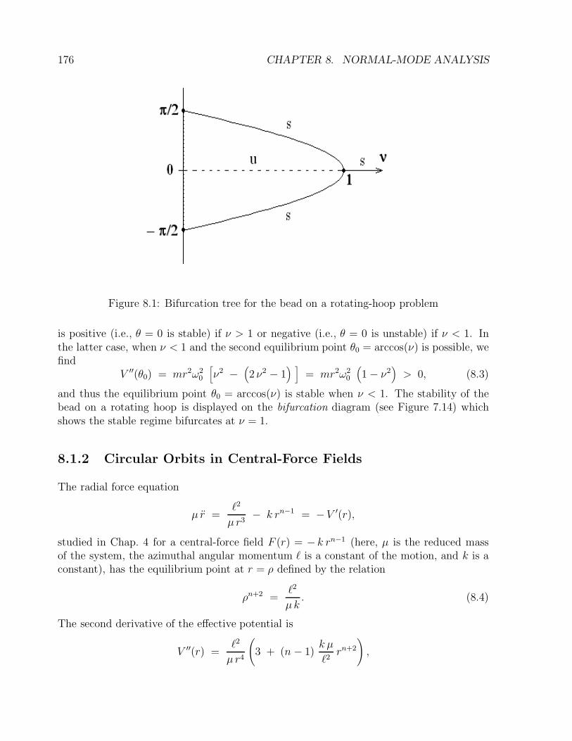
176 CHAPTER 8. NORMAL-MODE ANALYSIS
Figure 8.1: Bifurcation tree for the bead on a rotating-hoop problem
is positive (i.e., θ = 0 is stable) if ν > 1 or negative (i.e., θ = 0 is unstable) if ν < 1. Inthe latter case, when ν < 1 and the second equilibrium point θ0 = arccos(ν) is possible, wefind
V ′′(θ0) = mr2ω20
[ν2 −
(2 ν2 − 1
) ]= mr2ω2
0
(1 − ν2
)> 0, (8.3)
and thus the equilibrium point θ0 = arccos(ν) is stable when ν < 1. The stability of thebead on a rotating hoop is displayed on the bifurcation diagram (see Figure 7.14) whichshows the stable regime bifurcates at ν = 1.
8.1.2 Circular Orbits in Central-Force Fields
The radial force equation
µ r =`2
µr3− k rn−1 = −V ′(r),
studied in Chap. 4 for a central-force field F (r) = − k rn−1 (here, µ is the reduced massof the system, the azimuthal angular momentum ` is a constant of the motion, and k is aconstant), has the equilibrium point at r = ρ defined by the relation
ρn+2 =`2
µk. (8.4)
The second derivative of the effective potential is
V ′′(r) =`2
µr4
(
3 + (n − 1)k µ
`2rn+2
)
,
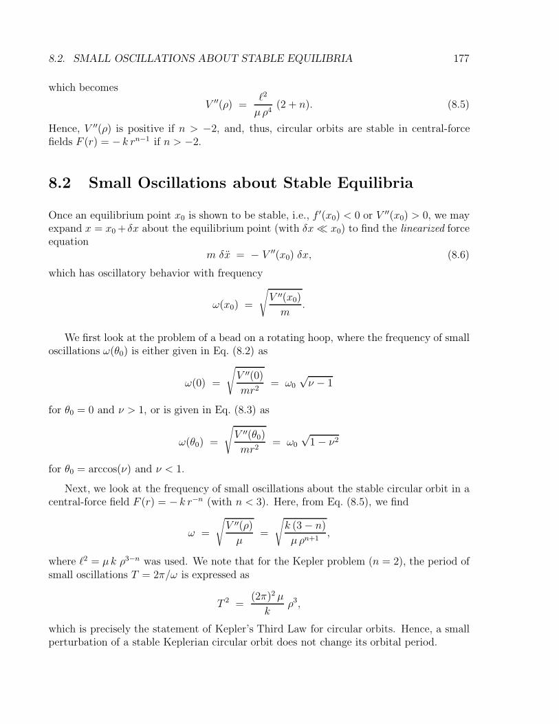
8.2. SMALL OSCILLATIONS ABOUT STABLE EQUILIBRIA 177
which becomes
V ′′(ρ) =`2
µρ4(2 + n). (8.5)
Hence, V ′′(ρ) is positive if n > −2, and, thus, circular orbits are stable in central-forcefields F (r) = − k rn−1 if n > −2.
8.2 Small Oscillations about Stable Equilibria
Once an equilibrium point x0 is shown to be stable, i.e., f ′(x0) < 0 or V ′′(x0) > 0, we mayexpand x = x0 + δx about the equilibrium point (with δx x0) to find the linearized forceequation
m δx = − V ′′(x0) δx, (8.6)
which has oscillatory behavior with frequency
ω(x0) =
√V ′′(x0)
m.
We first look at the problem of a bead on a rotating hoop, where the frequency of smalloscillations ω(θ0) is either given in Eq. (8.2) as
ω(0) =
√V ′′(0)
mr2= ω0
√ν − 1
for θ0 = 0 and ν > 1, or is given in Eq. (8.3) as
ω(θ0) =
√V ′′(θ0)
mr2= ω0
√1 − ν2
for θ0 = arccos(ν) and ν < 1.
Next, we look at the frequency of small oscillations about the stable circular orbit in acentral-force field F (r) = − k r−n (with n < 3). Here, from Eq. (8.5), we find
ω =
√V ′′(ρ)
µ=
√k (3 − n)
µρn+1,
where `2 = µk ρ3−n was used. We note that for the Kepler problem (n = 2), the period ofsmall oscillations T = 2π/ω is expressed as
T 2 =(2π)2 µ
kρ3,
which is precisely the statement of Kepler’s Third Law for circular orbits. Hence, a smallperturbation of a stable Keplerian circular orbit does not change its orbital period.
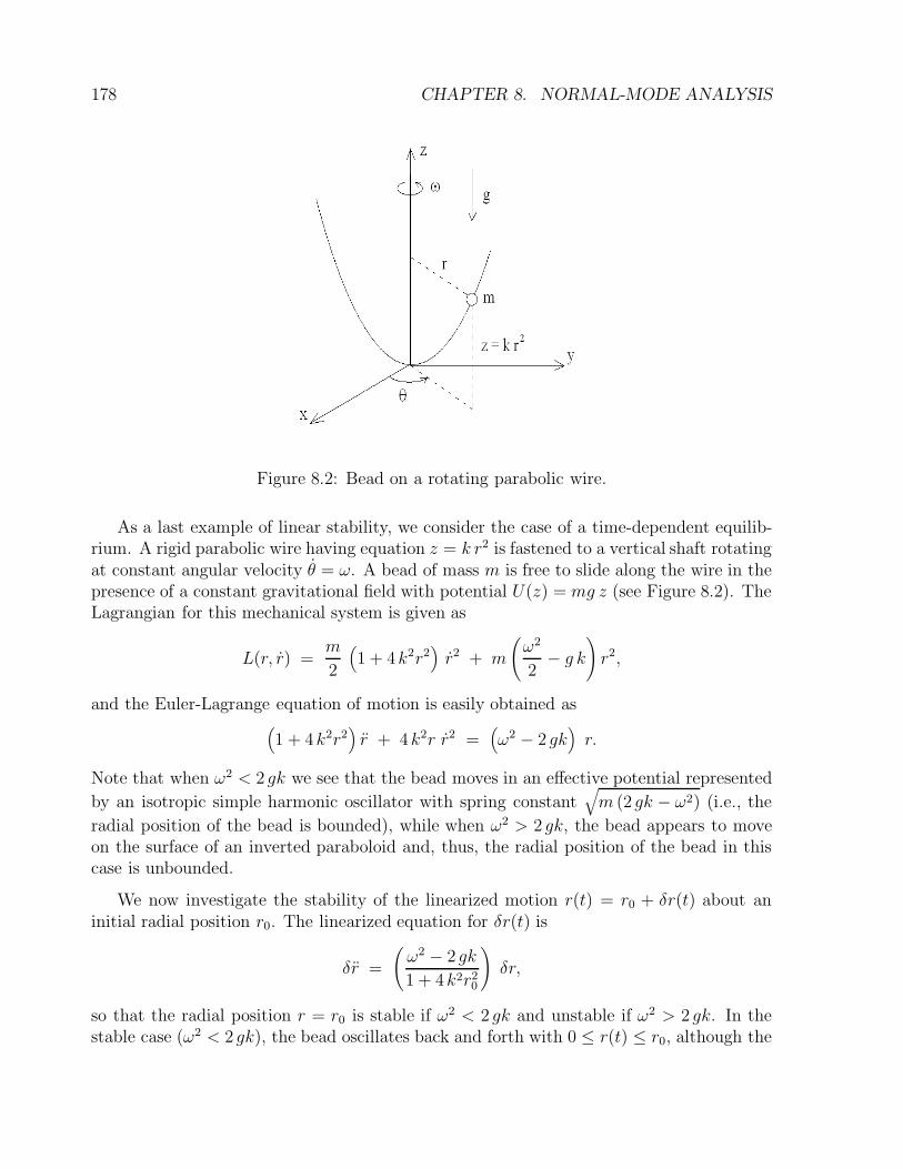
178 CHAPTER 8. NORMAL-MODE ANALYSIS
Figure 8.2: Bead on a rotating parabolic wire.
As a last example of linear stability, we consider the case of a time-dependent equilib-rium. A rigid parabolic wire having equation z = k r2 is fastened to a vertical shaft rotatingat constant angular velocity θ = ω. A bead of mass m is free to slide along the wire in thepresence of a constant gravitational field with potential U(z) = mg z (see Figure 8.2). TheLagrangian for this mechanical system is given as
L(r, r) =m
2
(1 + 4k2r2
)r2 + m
(ω2
2− g k
)
r2,
and the Euler-Lagrange equation of motion is easily obtained as(1 + 4k2r2
)r + 4k2r r2 =
(ω2 − 2 gk
)r.
Note that when ω2 < 2 gk we see that the bead moves in an effective potential represented
by an isotropic simple harmonic oscillator with spring constant√m (2 gk − ω2) (i.e., the
radial position of the bead is bounded), while when ω2 > 2 gk, the bead appears to moveon the surface of an inverted paraboloid and, thus, the radial position of the bead in thiscase is unbounded.
We now investigate the stability of the linearized motion r(t) = r0 + δr(t) about aninitial radial position r0. The linearized equation for δr(t) is
δr =
(ω2 − 2 gk
1 + 4k2r20
)
δr,
so that the radial position r = r0 is stable if ω2 < 2 gk and unstable if ω2 > 2 gk. In thestable case (ω2 < 2 gk), the bead oscillates back and forth with 0 ≤ r(t) ≤ r0, although the
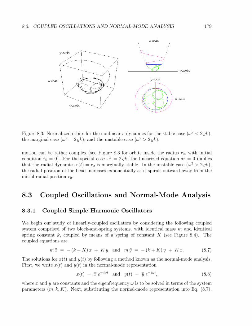
8.3. COUPLED OSCILLATIONS AND NORMAL-MODE ANALYSIS 179
Figure 8.3: Normalized orbits for the nonlinear r-dynamics for the stable case (ω2 < 2 gk),the marginal case (ω2 = 2 gk), and the unstable case (ω2 > 2 gk).
motion can be rather complex (see Figure 8.3 for orbits inside the radius r0, with initialcondition r0 = 0). For the special case ω2 = 2 gk, the linearized equation δr = 0 impliesthat the radial dynamics r(t) = r0 is marginally stable. In the unstable case (ω2 > 2 gk),the radial position of the bead increases exponentially as it spirals outward away from theinitial radial position r0.
8.3 Coupled Oscillations and Normal-Mode Analysis
8.3.1 Coupled Simple Harmonic Oscillators
We begin our study of linearily-coupled oscillators by considering the following coupledsystem comprised of two block-and-spring systems, with identical mass m and identicalspring constant k, coupled by means of a spring of constant K (see Figure 8.4). Thecoupled equations are
mx = − (k +K)x + K y and m y = − (k +K) y + K x. (8.7)
The solutions for x(t) and y(t) by following a method known as the normal-mode analysis.First, we write x(t) and y(t) in the normal-mode representation
x(t) = x e− iωt and y(t) = y e− iωt, (8.8)
where x and y are constants and the eigenfrequency ω is to be solved in terms of the systemparameters (m, k,K). Next, substituting the normal-mode representation into Eq. (8.7),

180 CHAPTER 8. NORMAL-MODE ANALYSIS
Figure 8.4: Coupled identical masses and springs
we obtain the following normal-mode matrix equation(ω2m− (k +K) K
K ω2 m− (k +K)
)(xy
)
= 0. (8.9)
To obtain a non-trivial solution x, y 6= 0, the determinant of the matrix in Eq. (8.9) isrequired to vanish, which yields the characteristic polynomial
[ω2m− (k +K)]2 − K2 = 0,
whose solutions are the eigenfrequencies
ω2± =
(k +K)
m± K
m.
If we insert ω2+ = (k + 2K)/m into the matrix equation (8.9), we find
(K KK K
)(xy
)
= 0,
which implies that y = −x, and thus the eigenfrequency ω+ is associated with an anti-symmetric coupled motion. If we insert ω2
− = k/m into the matrix equation (8.9), wefind (
−K KK −K
)(xy
)
= 0,
which implies that y = x, and thus the eigenfrequency ω− is associated with a symmetriccoupled motion.
Figures 8.5 and 8.6 show the normalized solutions of the coupled equations (8.7), where
time is normalized as t →√k/m t, for the weak coupling (K < k) and strong coupling
(K > k) cases, respectively. Note that the two eigenfrequencies are said to be commen-
surate if the ratio ω+/Ω− =√
1 + 2K/k is expressed as a rational number ρ for values of
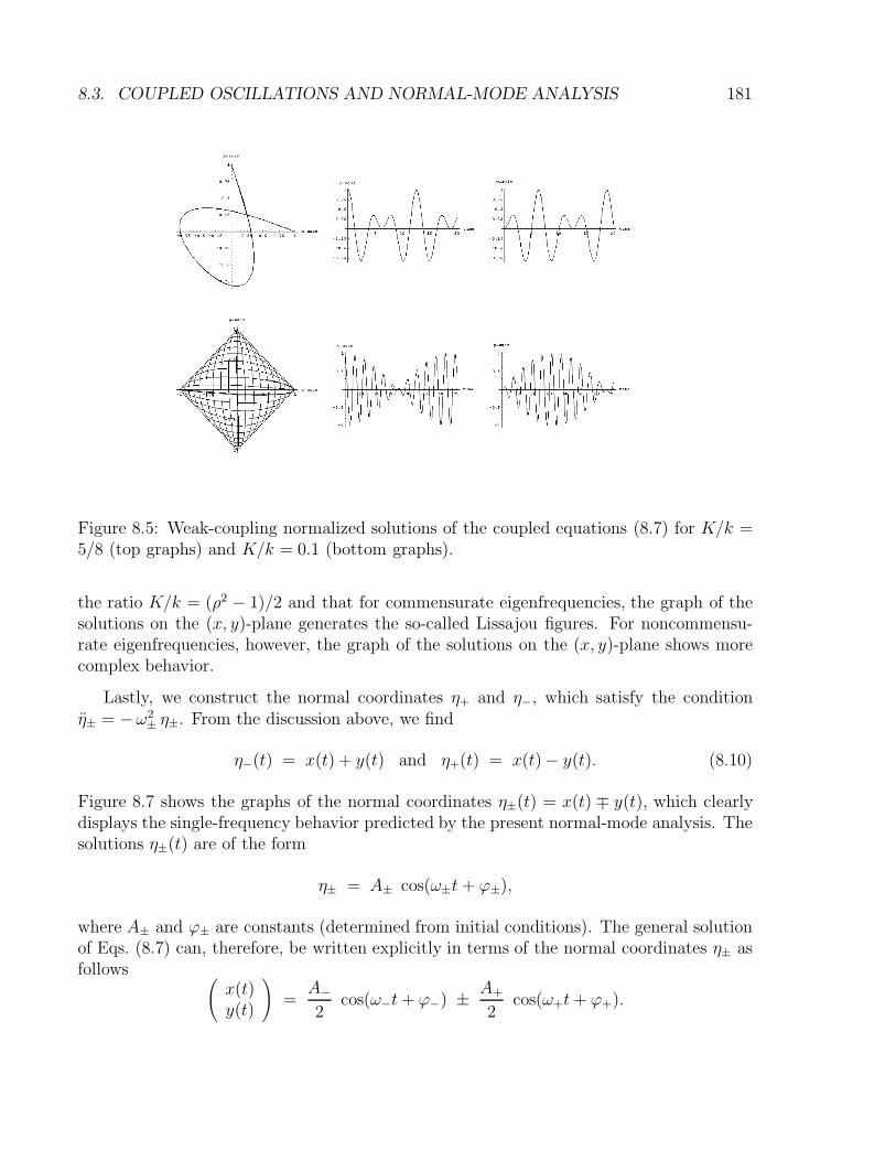
8.3. COUPLED OSCILLATIONS AND NORMAL-MODE ANALYSIS 181
Figure 8.5: Weak-coupling normalized solutions of the coupled equations (8.7) for K/k =5/8 (top graphs) and K/k = 0.1 (bottom graphs).
the ratio K/k = (ρ2 − 1)/2 and that for commensurate eigenfrequencies, the graph of thesolutions on the (x, y)-plane generates the so-called Lissajou figures. For noncommensu-rate eigenfrequencies, however, the graph of the solutions on the (x, y)-plane shows morecomplex behavior.
Lastly, we construct the normal coordinates η+ and η−, which satisfy the conditionη± = −ω2
± η±. From the discussion above, we find
η−(t) = x(t) + y(t) and η+(t) = x(t)− y(t). (8.10)
Figure 8.7 shows the graphs of the normal coordinates η±(t) = x(t) ∓ y(t), which clearlydisplays the single-frequency behavior predicted by the present normal-mode analysis. Thesolutions η±(t) are of the form
η± = A± cos(ω±t+ ϕ±),
where A± and ϕ± are constants (determined from initial conditions). The general solutionof Eqs. (8.7) can, therefore, be written explicitly in terms of the normal coordinates η± asfollows (
x(t)y(t)
)
=A−2
cos(ω−t+ ϕ−) ± A+
2cos(ω+t+ ϕ+).
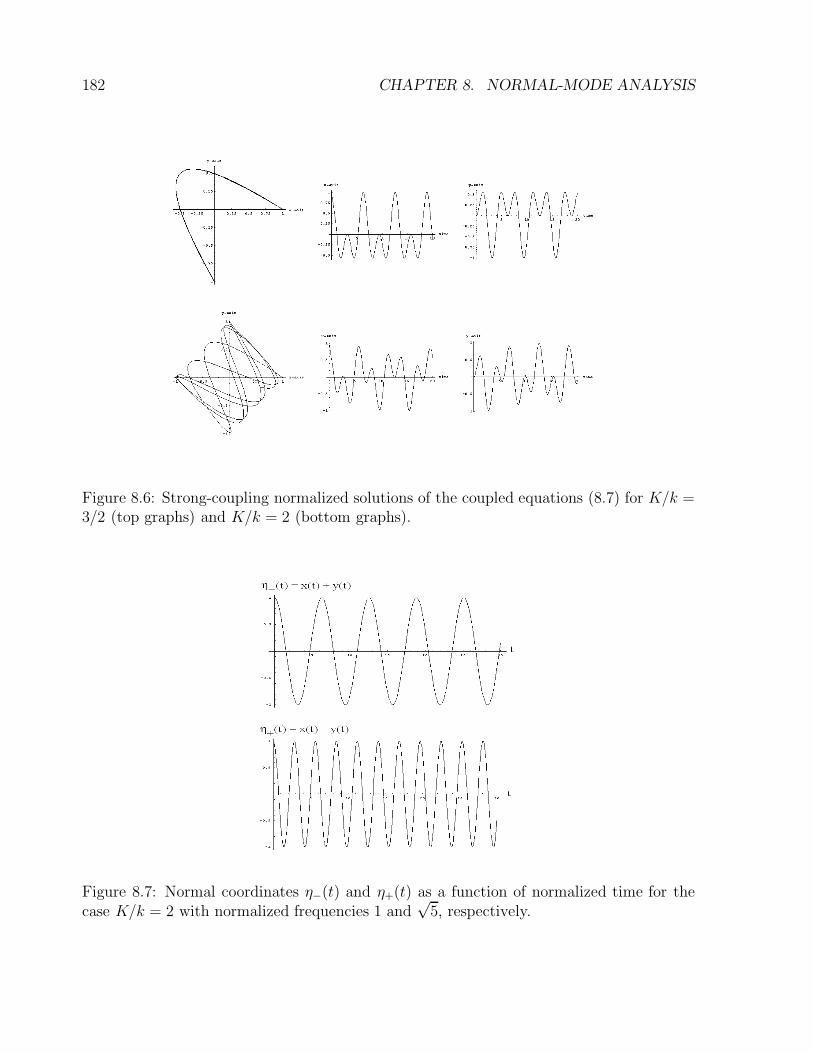
182 CHAPTER 8. NORMAL-MODE ANALYSIS
Figure 8.6: Strong-coupling normalized solutions of the coupled equations (8.7) for K/k =3/2 (top graphs) and K/k = 2 (bottom graphs).
Figure 8.7: Normal coordinates η−(t) and η+(t) as a function of normalized time for thecase K/k = 2 with normalized frequencies 1 and
√5, respectively.
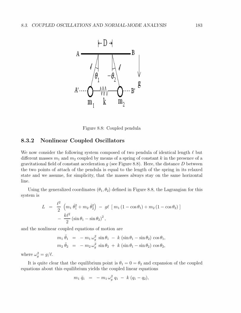
8.3. COUPLED OSCILLATIONS AND NORMAL-MODE ANALYSIS 183
Figure 8.8: Coupled pendula
8.3.2 Nonlinear Coupled Oscillators
We now consider the following system composed of two pendula of identical length ` butdifferent masses m1 and m2 coupled by means of a spring of constant k in the presence of agravitational field of constant acceleration g (see Figure 8.8). Here, the distance D betweenthe two points of attach of the pendula is equal to the length of the spring in its relaxedstate and we assume, for simplicity, that the masses always stay on the same horizontalline.
Using the generalized coordinates (θ1, θ2) defined in Figure 8.8, the Lagrangian for thissystem is
L =`2
2
(m1 θ
21 +m2 θ
22
)− g` [ m1 (1 − cos θ1) +m2 (1 − cos θ2) ]
− k`2
2(sin θ1 − sin θ2)
2,
and the nonlinear coupled equations of motion are
m1 θ1 = − m1 ω2g sin θ1 − k (sin θ1 − sin θ2) cos θ1,
m2 θ2 = − m2 ω2g sin θ2 + k (sin θ1 − sin θ2) cos θ2,
where ω2g = g/`.
It is quite clear that the equilibrium point is θ1 = 0 = θ2 and expansion of the coupledequations about this equilibrium yields the coupled linear equations
m1 q1 = − m1 ω2g q1 − k (q1 − q2),

184 CHAPTER 8. NORMAL-MODE ANALYSIS
m2 q2 = − m2 ω2g q2 + k (q1 − q2),
where θ1 = q1 1 and θ2 = q2 1. The normal-mode matrix associated with thesecoupled linear equations is
((ω2 − ω2
g)m1 − k kk (ω2 − ω2
g)m2 − k
)(q1q2
)
= 0,
and the characteristic polynomial is
M[
(ω2 − ω2g)µ − k
](ω2 − ω2
g) = 0,
where µ = m1m2/M is the reduced mass for the system and M = m1 + m2 is the totalmass. The eigenfrequencies are thus
ω2− = ω2
g and ω2+ = ω2
g +k
µ.
The normal coordinates η± are expressed in terms of (q1, q2) as η± = a± q1+b± q2, wherea± and b± are constant coefficients determined from the condition η± = −ω2
± η±. Fromthis condition we find
(k
m1+ ω2
g
)
− b±a±
k
m2= ω2
± =
(k
m2+ ω2
g
)
− a±b±
k
m1.
For the eigenfrequency ω2− = ω2
g , we find b−/a− = m2/m1, and thus we may choose
η− =m1
Mq1 +
m2
Mq2,
which represents the center of mass position for the system. For the eigenfrequency ω2+ =
ωg + k/µ, we find b+/a+ = − 1, and thus we may choose
η+ = q1 − q2.
Lastly, we may solve for q1 and q2 as
q1 = η− +m2
Mη+ and q2 = η− − m1
Mη+,
where η± = A± cos(ω± t + ϕ±) are general solutions of the normal-mode equations η± =−ω2
± η±.
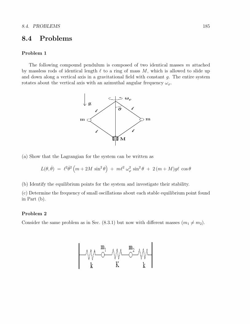
8.4. PROBLEMS 185
8.4 Problems
Problem 1
The following compound pendulum is composed of two identical masses m attachedby massless rods of identical length ` to a ring of mass M , which is allowed to slide upand down along a vertical axis in a gravitational field with constant g. The entire systemrotates about the vertical axis with an azimuthal angular frequency ωϕ.
(a) Show that the Lagrangian for the system can be written as
L(θ, θ) = `2θ2(m+ 2M sin2 θ
)+ m`2 ω2
ϕ sin2 θ + 2 (m+M)g` cos θ
(b) Identify the equilibrium points for the system and investigate their stability.
(c) Determine the frequency of small oscillations about each stable equilibrium point foundin Part (b).
Problem 2
Consider the same problem as in Sec. (8.3.1) but now with different masses (m1 6= m2).
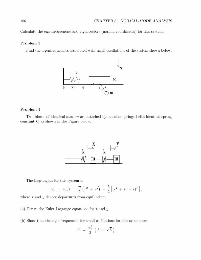
186 CHAPTER 8. NORMAL-MODE ANALYSIS
Calculate the eigenfrequencies and eigenvectors (normal coordinates) for this system.
Problem 3
Find the eigenfrequencies associated with small oscillations of the system shown below.
Problem 4
Two blocks of identical mass m are attached by massless springs (with identical springconstant k) as shown in the Figure below.
The Lagrangian for this system is
L(x, x; y, y) =m
2
(x2 + y2
)− k
2
[x2 + (y − x)2
],
where x and y denote departures from equilibrium.
(a) Derive the Euler-Lagrange equations for x and y.
(b) Show that the eigenfrequencies for small oscillations for this system are
ω2± =
ω2k
2
(3 ±
√5),
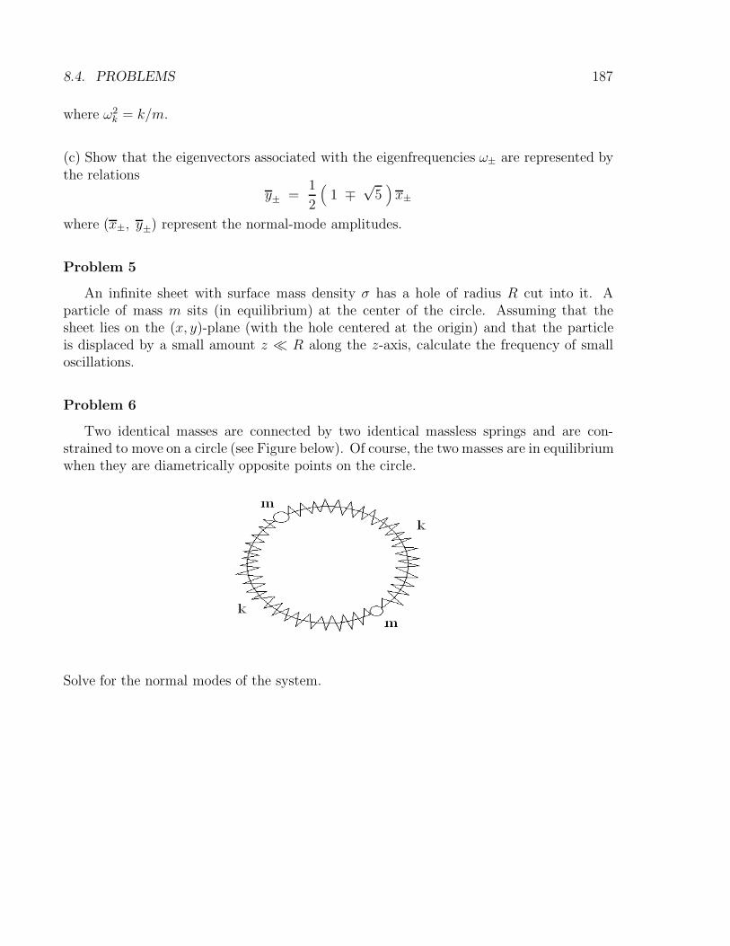
8.4. PROBLEMS 187
where ω2k = k/m.
(c) Show that the eigenvectors associated with the eigenfrequencies ω± are represented bythe relations
y± =1
2
(1 ∓
√5)x±
where (x±, y±) represent the normal-mode amplitudes.
Problem 5
An infinite sheet with surface mass density σ has a hole of radius R cut into it. Aparticle of mass m sits (in equilibrium) at the center of the circle. Assuming that thesheet lies on the (x, y)-plane (with the hole centered at the origin) and that the particleis displaced by a small amount z R along the z-axis, calculate the frequency of smalloscillations.
Problem 6
Two identical masses are connected by two identical massless springs and are con-strained to move on a circle (see Figure below). Of course, the two masses are in equilibriumwhen they are diametrically opposite points on the circle.
Solve for the normal modes of the system.
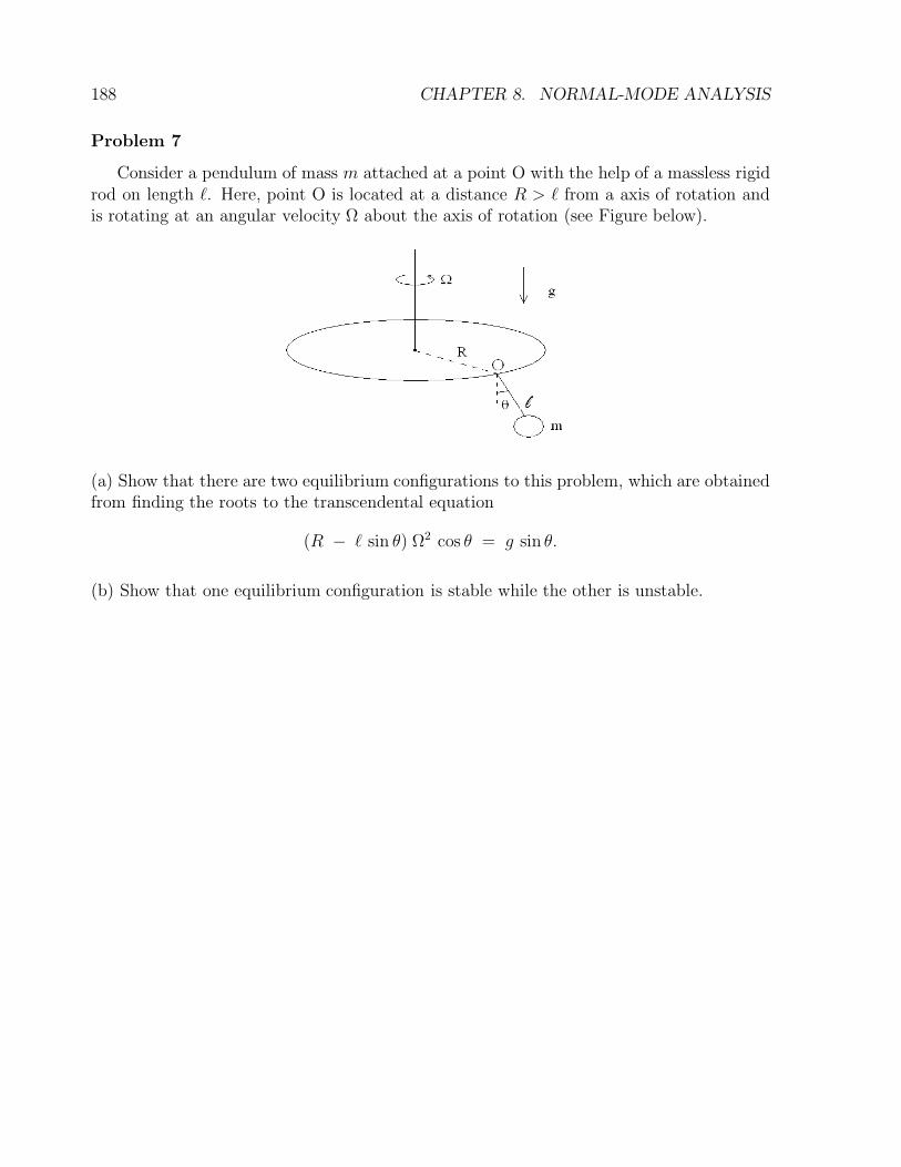
188 CHAPTER 8. NORMAL-MODE ANALYSIS
Problem 7
Consider a pendulum of mass m attached at a point O with the help of a massless rigidrod on length `. Here, point O is located at a distance R > ` from a axis of rotation andis rotating at an angular velocity Ω about the axis of rotation (see Figure below).
(a) Show that there are two equilibrium configurations to this problem, which are obtainedfrom finding the roots to the transcendental equation
(R − ` sin θ) Ω2 cos θ = g sin θ.
(b) Show that one equilibrium configuration is stable while the other is unstable.
Chapter 9
Continuous Lagrangian Systems
9.1 Waves on a Stretched String
9.1.1 Wave Equation
The equation describing waves propagating on a stretched string of constant linear massdensity ρ under constant tension T is
ρ∂2u(x, t)
∂t2= T
∂2u(x, t)
∂x2, (9.1)
where u(x, t) denotes the amplitude of the wave at position x along the string at time t.
General solutions to this equation involve arbitrary functions g(x± v t), where v =√T/ρ
represents the speed of waves propagating on the string. Indeed, we find
ρ ∂2t g(x± v t) = ρ v2 g′′ = T g′′ = T ∂2
xg(x± v t).
The interpretation of the two different signs is that g(x−v t) represents a wave propagatingto the right while g(x+v t) represents a wave propagating to the left. The general solutionof the wave equation (9.1) is
u(x, t) = A− g(x− v t) + A+ g(x+ v t),
where A± are arbitrary constants.
9.1.2 Lagrangian Formalism
The question we now ask is whether the wave equation (9.1) can be derived from a varia-tional principle
δ∫
L(u, ∂tu, ∂xu; x, t) dx dt = 0, (9.2)
189
190 CHAPTER 9. CONTINUOUS LAGRANGIAN SYSTEMS
where the Lagrangian density L(u, ∂tu, ∂xu; x, t) is a function of the dynamical variableu(x, t) and its space-time derivatives. Here, the variation of the Lagrangian density L isexpressed as
δL = δu∂L∂u
+ ∂tδu∂L
∂(∂tu)+ ∂xδu
∂L∂(∂xu)
,
where δu(x, t) is a general variation of u(x, t) subject to the condition that it vanishes atthe integration boundaries in Eq. (9.2). By re-arranging terms, the variation of L can bewritten as
δL = δu
∂L∂u
− ∂
∂t
(∂L
∂(∂tu)
)
− ∂
∂x
(∂L
∂(∂xu)
)
+∂
∂t
(
δu∂L
∂(∂tu)
)
+∂
∂x
(
δu∂L
∂(∂xu)
)
. (9.3)
When we insert this expression for δL into the variational principle (9.2), we obtain
∫dx dt δu
∂L∂u
− ∂
∂t
(∂L
∂(∂tu)
)
− ∂
∂x
(∂L
∂(∂xu)
)
= 0, (9.4)
where the last two terms in Eq. (9.3) cancel out because δu vanishes on the integrationboundaries. Since the variational principle (9.4) is true for general variations δu, we obtainthe Euler-Lagrange equation for the dynamical field u(x, t):
∂
∂t
(∂L
∂(∂tu)
)
+∂
∂x
(∂L
∂(∂xu)
)
=∂L∂u
. (9.5)
9.1.3 Lagrangian Description for Waves on a Stretched String
The question we posed earlier now focuses on deciding what form the Lagrangian densitymust take. Here, the answer is surprisingly simple: the kinetic energy density of the waveis ρ (∂tu)
2/2, while the potential energy density is T (∂xu)2/2, and thus the Lagrangian
density for waves on a stretched string is
L(u, ∂tu, ∂xu; x, t) =ρ
2
(∂u
∂t
)2
− T
2
(∂u
∂x
)2
. (9.6)
Since ∂L/∂u = 0, we find
∂
∂t
(∂L
∂(∂tu)
)
=∂
∂t
(
ρ∂u
∂t
)
= ρ∂2u
∂t2,
∂
∂x
(∂L
∂(∂xu)
)
=∂
∂x
(
− T∂u
∂x
)
= − T∂2u
∂x2,

9.2. GENERAL VARIATIONAL PRINCIPLE FOR FIELD THEORY* 191
and Eq. (9.1) is indeed represented as an Euler-Lagrange equation (9.5) in terms of theLagrangian density (9.6).
The energy density E of a stretched string can also be calculated by using the Legendretransformation
E ≡ ∂u
∂t
∂L∂(∂tu)
− L =ρ
2
(∂u
∂t
)2
+T
2
(∂u
∂x
)2
.
By using the wave equation (9.1), we readily find that the time derivative of the energydensity
∂E∂t
=∂
∂x
(
T∂u
∂t
∂u
∂x
)
can be expressed as an energy conservation law ∂tE + ∂S = 0, where the energy-densityflux is defined as S ≡ −T ∂xu ∂tu. The next Section will present the general variationalformulation of classical field theory, which will enable to show that the wave equation (9.1)also satisfies the momentum conservation law ∂tP+∂xE = 0, where the momentum densityis P ≡ S/v2.
9.2 General Variational Principle for Field Theory*
The simple example of waves on a stretched string allows us to view the Euler-Lagrangeequation (9.5) as a generalization of the Euler-Lagrange equations
d
dt
(∂L
∂qi
)
=∂L
∂qi,
in terms of the generalized coordinates qi. We now spend some time investigating theLagrangian description of continuous systems, in which the dynamical variables are fieldsψ(x, t) instead of spatial coordinates x.
9.2.1 Action Functional
Classical and quantum field theories rely on variational principles based on the existenceof action functionals. The typical action functional is of the form
A[ψ] =∫d4x L(ψ, ∂µψ), (9.7)
where the wave function ψ(x, t) represents the state of the system at position x and timet while the entire physical content of the theory is carried by the Lagrangian density L.
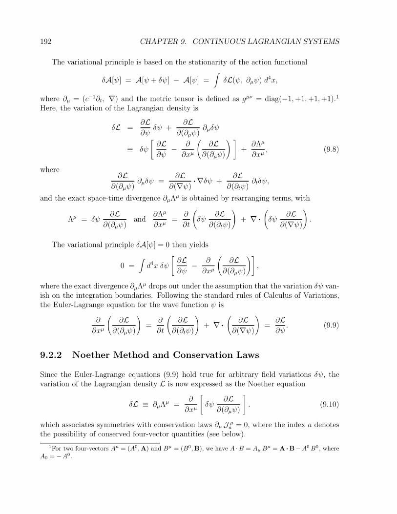
192 CHAPTER 9. CONTINUOUS LAGRANGIAN SYSTEMS
The variational principle is based on the stationarity of the action functional
δA[ψ] = A[ψ + δψ] − A[ψ] =∫δL(ψ, ∂µψ) d4x,
where ∂µ = (c−1∂t, ∇) and the metric tensor is defined as gµν = diag(−1,+1,+1,+1).1
Here, the variation of the Lagrangian density is
δL =∂L∂ψ
δψ +∂L
∂(∂µψ)∂µδψ
≡ δψ
[∂L∂ψ
− ∂
∂xµ
(∂L
∂(∂µψ)
) ]
+∂Λµ
∂xµ, (9.8)
where∂L
∂(∂µψ)∂µδψ =
∂L∂(∇ψ)
·∇δψ +∂L
∂(∂tψ)∂tδψ,
and the exact space-time divergence ∂µΛµ is obtained by rearranging terms, with
Λµ = δψ∂L
∂(∂µψ)and
∂Λµ
∂xµ=
∂
∂t
(
δψ∂L
∂(∂tψ)
)
+ ∇ ·
(
δψ∂L
∂(∇ψ)
)
.
The variational principle δA[ψ] = 0 then yields
0 =∫d4x δψ
[∂L∂ψ
− ∂
∂xµ
(∂L
∂(∂µψ)
)]
,
where the exact divergence ∂µΛµ drops out under the assumption that the variation δψ van-
ish on the integration boundaries. Following the standard rules of Calculus of Variations,the Euler-Lagrange equation for the wave function ψ is
∂
∂xµ
(∂L
∂(∂µψ)
)
=∂
∂t
(∂L
∂(∂tψ)
)
+ ∇ ·
(∂L
∂(∇ψ)
)
=∂L∂ψ
. (9.9)
9.2.2 Noether Method and Conservation Laws
Since the Euler-Lagrange equations (9.9) hold true for arbitrary field variations δψ, thevariation of the Lagrangian density L is now expressed as the Noether equation
δL ≡ ∂µΛµ =
∂
∂xµ
[
δψ∂L
∂(∂µψ)
]
. (9.10)
which associates symmetries with conservation laws ∂µJ µa = 0, where the index a denotes
the possibility of conserved four-vector quantities (see below).
1For two four-vectors Aµ = (A0, A) and Bµ = (B0, B), we have A ·B = Aµ Bµ = A ·B−A0 B0 , whereA0 = −A0.
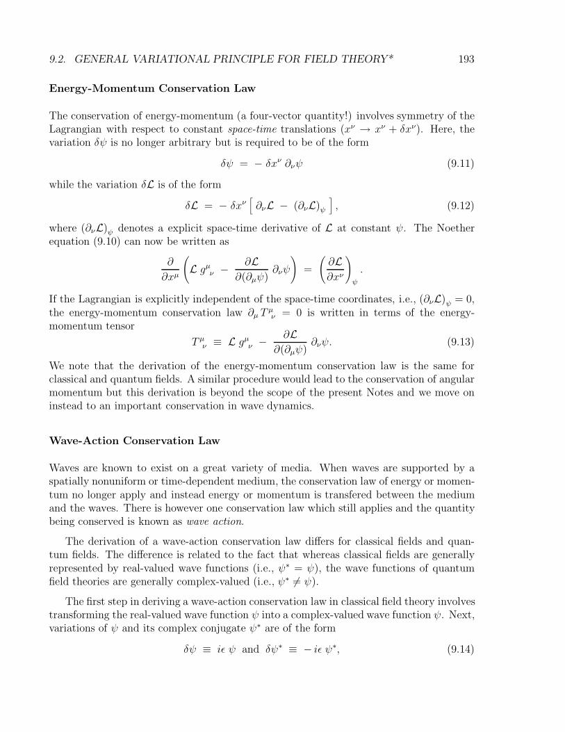
9.2. GENERAL VARIATIONAL PRINCIPLE FOR FIELD THEORY* 193
Energy-Momentum Conservation Law
The conservation of energy-momentum (a four-vector quantity!) involves symmetry of theLagrangian with respect to constant space-time translations (xν → xν + δxν). Here, thevariation δψ is no longer arbitrary but is required to be of the form
δψ = − δxν ∂νψ (9.11)
while the variation δL is of the form
δL = − δxν[∂νL − (∂νL)ψ
], (9.12)
where (∂νL)ψ denotes a explicit space-time derivative of L at constant ψ. The Noetherequation (9.10) can now be written as
∂
∂xµ
(
L gµν − ∂L∂(∂µψ)
∂νψ
)
=
(∂L∂xν
)
ψ
.
If the Lagrangian is explicitly independent of the space-time coordinates, i.e., (∂νL)ψ = 0,the energy-momentum conservation law ∂µ T
µν = 0 is written in terms of the energy-
momentum tensor
T µν ≡ L gµν − ∂L∂(∂µψ)
∂νψ. (9.13)
We note that the derivation of the energy-momentum conservation law is the same forclassical and quantum fields. A similar procedure would lead to the conservation of angularmomentum but this derivation is beyond the scope of the present Notes and we move oninstead to an important conservation in wave dynamics.
Wave-Action Conservation Law
Waves are known to exist on a great variety of media. When waves are supported by aspatially nonuniform or time-dependent medium, the conservation law of energy or momen-tum no longer apply and instead energy or momentum is transfered between the mediumand the waves. There is however one conservation law which still applies and the quantitybeing conserved is known as wave action.
The derivation of a wave-action conservation law differs for classical fields and quan-tum fields. The difference is related to the fact that whereas classical fields are generallyrepresented by real-valued wave functions (i.e., ψ∗ = ψ), the wave functions of quantumfield theories are generally complex-valued (i.e., ψ∗ 6= ψ).
The first step in deriving a wave-action conservation law in classical field theory involvestransforming the real-valued wave function ψ into a complex-valued wave function ψ. Next,variations of ψ and its complex conjugate ψ∗ are of the form
δψ ≡ iε ψ and δψ∗ ≡ − iε ψ∗, (9.14)

194 CHAPTER 9. CONTINUOUS LAGRANGIAN SYSTEMS
Lastly, we transform the classical Lagrangian density L into a real-valued Lagrangian den-sity LR(ψ, ψ∗) such that δLR ≡ 0. The wave-action conservation law is, therefore,expressed in the form ∂µJ µ = 0, where the wave-action four-density is
J µ ≡ 2 Im
[
ψ∂LR∂(∂µψ)
]
, (9.15)
where Im[· · ·] denotes the imaginary part.
9.3 Variational Principle for Schroedinger Equation*
A simple yet important example for a quantum field theory is provided by the Schroedingerequation for a spinless particle of mass m subjected to a real-valued potential energyfunction V (x, t). The Lagrangian density for the Schroedinger equation is given as
LR = − h2
2m|∇ψ|2 +
ih
2
(
ψ∗ ∂ψ
∂t− ψ
∂ψ∗
∂t
)
− V |ψ|2. (9.16)
The Schroedinger equation for ψ is derived as an Euler-Lagrange equation (9.9) in termsof ψ∗, where
∂LR∂(∂tψ∗)
= − ih
2ψ → ∂
∂t
(∂LR
∂(∂tψ∗)
)
= − ih
2
∂ψ
∂t,
∂LR∂(∇ψ∗)
= − h2
2m∇ψ → ∇ ·
(∂LR
∂(∇ψ∗)
)
= − h2
2m∇2ψ,
∂LR∂ψ∗ =
ih
2
∂ψ
∂t− V ψ,
so that the Euler-Lagrange equation (9.9) for the Schroedinger Lagrangian (9.16) becomes
ih∂ψ
∂t= − h2
2m∇2ψ + V ψ, (9.17)
where the Schroedinger equation for ψ∗ is as an Euler-Lagrange equation (9.9) in terms ofψ, which yields
− ih∂ψ∗
∂t= − h2
2m∇2ψ∗ + V ψ∗, (9.18)
which is simply the complex-conjugate equation of Eq. (9.17).
The energy-momentum conservation law is now derived by Noether method. Becausethe potential V (x, t) is spatially nonuniform and time dependent, the energy-momentumcontained in the wave field is not conserved and energy-momentum is exchanged between
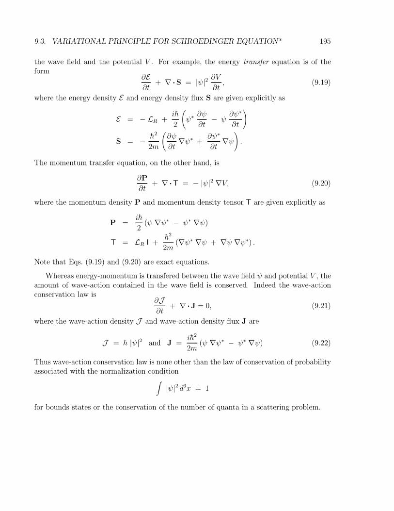
9.3. VARIATIONAL PRINCIPLE FOR SCHROEDINGER EQUATION* 195
the wave field and the potential V . For example, the energy transfer equation is of theform
∂E∂t
+ ∇ ·S = |ψ|2 ∂V∂t, (9.19)
where the energy density E and energy density flux S are given explicitly as
E = − LR +ih
2
(
ψ∗ ∂ψ
∂t− ψ
∂ψ∗
∂t
)
S = − h2
2m
(∂ψ
∂t∇ψ∗ +
∂ψ∗
∂t∇ψ
)
.
The momentum transfer equation, on the other hand, is
∂P
∂t+ ∇ ·T = − |ψ|2 ∇V, (9.20)
where the momentum density P and momentum density tensor T are given explicitly as
P =ih
2(ψ ∇ψ∗ − ψ∗ ∇ψ)
T = LR I +h2
2m(∇ψ∗ ∇ψ + ∇ψ ∇ψ∗) .
Note that Eqs. (9.19) and (9.20) are exact equations.
Whereas energy-momentum is transfered between the wave field ψ and potential V , theamount of wave-action contained in the wave field is conserved. Indeed the wave-actionconservation law is
∂J∂t
+ ∇ ·J = 0, (9.21)
where the wave-action density J and wave-action density flux J are
J = h |ψ|2 and J =ih2
2m(ψ ∇ψ∗ − ψ∗ ∇ψ) (9.22)
Thus wave-action conservation law is none other than the law of conservation of probabilityassociated with the normalization condition
∫|ψ|2 d3x = 1
for bounds states or the conservation of the number of quanta in a scattering problem.

196 CHAPTER 9. CONTINUOUS LAGRANGIAN SYSTEMS
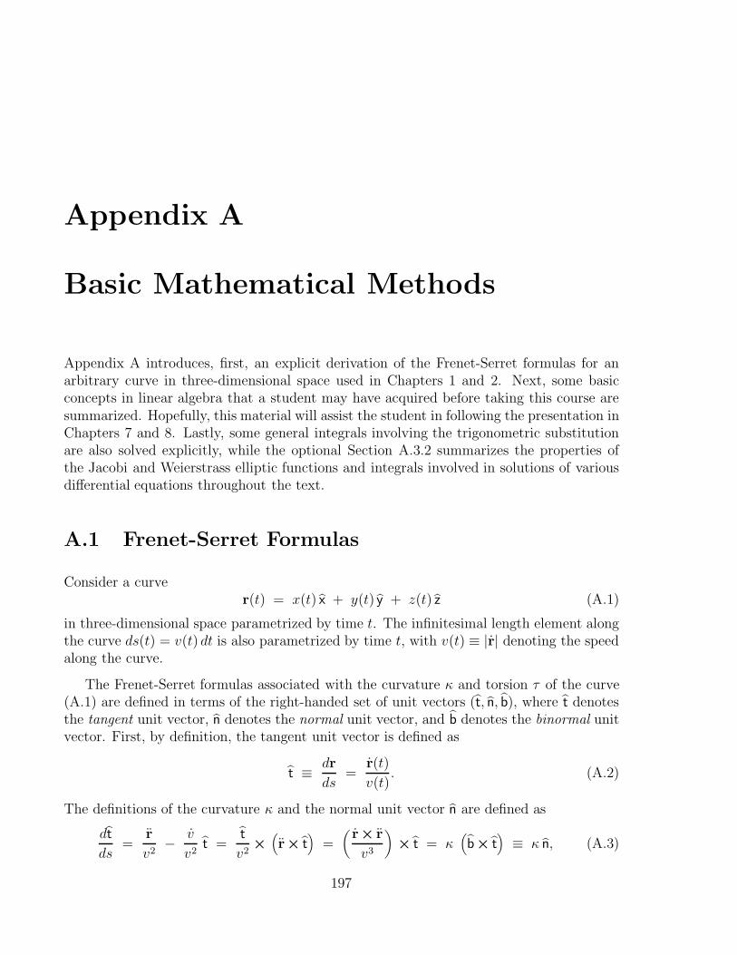
Appendix A
Basic Mathematical Methods
Appendix A introduces, first, an explicit derivation of the Frenet-Serret formulas for anarbitrary curve in three-dimensional space used in Chapters 1 and 2. Next, some basicconcepts in linear algebra that a student may have acquired before taking this course aresummarized. Hopefully, this material will assist the student in following the presentation inChapters 7 and 8. Lastly, some general integrals involving the trigonometric substitutionare also solved explicitly, while the optional Section A.3.2 summarizes the properties ofthe Jacobi and Weierstrass elliptic functions and integrals involved in solutions of variousdifferential equations throughout the text.
A.1 Frenet-Serret Formulas
Consider a curver(t) = x(t) x + y(t) y + z(t) z (A.1)
in three-dimensional space parametrized by time t. The infinitesimal length element alongthe curve ds(t) = v(t) dt is also parametrized by time t, with v(t) ≡ |r| denoting the speedalong the curve.
The Frenet-Serret formulas associated with the curvature κ and torsion τ of the curve(A.1) are defined in terms of the right-handed set of unit vectors (t, n, b), where t denotesthe tangent unit vector, n denotes the normal unit vector, and b denotes the binormal unitvector. First, by definition, the tangent unit vector is defined as
t ≡ dr
ds=
r(t)
v(t). (A.2)
The definitions of the curvature κ and the normal unit vector n are defined as
dt
ds=
r
v2− v
v2t =
t
v2×
(r× t
)=(r× r
v3
)× t = κ
(b× t
)≡ κ n, (A.3)
197
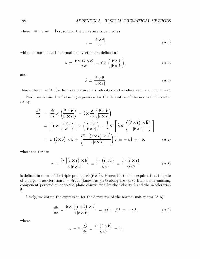
198 APPENDIX A. BASIC MATHEMATICAL METHODS
where v ≡ d|r|/dt = t · r, so that the curvature is defined as
κ ≡ |r× r|v3
, (A.4)
while the normal and binormal unit vectors are defined as
n ≡ r× (r× r)
κ v4= t ×
(r× r
|r× r|
)
, (A.5)
and
b ≡ r× r
|r× r| . (A.6)
Hence, the curve (A.1) exhibits curvature if its velocity r and acceleration r are not colinear.
Next, we obtain the following expression for the derivative of the normal unit vector(A.5):
dn
ds=
dt
ds×
(r× r
|r× r|
)
+ t ×d
ds
(r× r
|r× r|
)
=[
t ×
(r× r
v3
) ]×
(r× r
|r× r|
)
+t
v×
b×
(˙r × r
)× b
|r× r|
= κ(t × b
)× b +
t ·
[(˙r× r
)× b
]
v |r× r|
b ≡ − κ t + τ b, (A.7)
where the torsion
τ ≡t ·
[(˙r× r
)× b
]
v |r× r| =n ·
(˙r× r
)
κ v4=
r ·
(r × ˙r
)
κ2 v6(A.8)
is defined in terms of the triple product r · (r× ˙r). Hence, the torsion requires that the rateof change of acceleration ˙r = dr/dt (known as jerk) along the curve have a nonvanishingcomponent perpendicular to the plane constructed by the velocity r and the accelerationr.
Lastly, we obtain the expression for the derivative of the normal unit vector (A.6):
db
ds=
b ×
[(r× ˙r
)× b
]
v |r× r| = α t + β n ≡ − τ n, (A.9)
where
α ≡ t ·db
ds=
t ·
(r× ˙r
)
κ v4≡ 0,
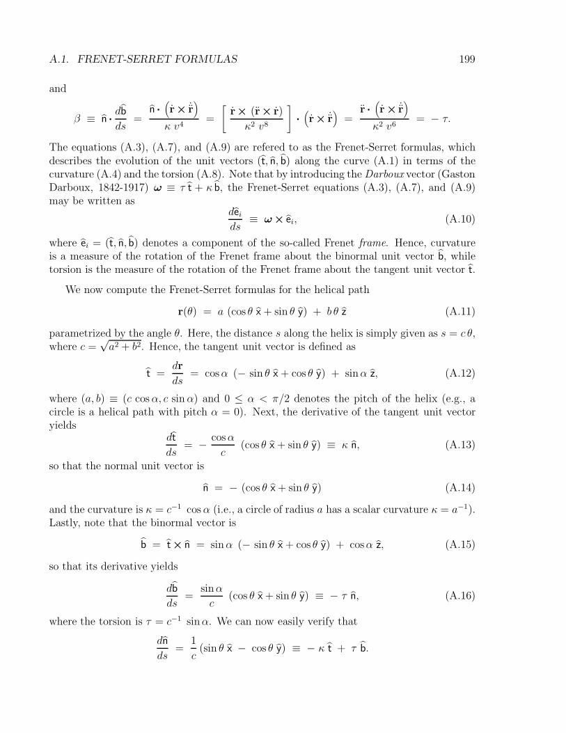
A.1. FRENET-SERRET FORMULAS 199
and
β ≡ n ·db
ds=
n ·
(r× ˙r
)
κ v4=
[r× (r× r)
κ2 v8
]
·
(r× ˙r
)=
r ·
(r × ˙r
)
κ2 v6= − τ.
The equations (A.3), (A.7), and (A.9) are refered to as the Frenet-Serret formulas, whichdescribes the evolution of the unit vectors (t, n, b) along the curve (A.1) in terms of thecurvature (A.4) and the torsion (A.8). Note that by introducing the Darboux vector (GastonDarboux, 1842-1917) ω ≡ τ t + κ b, the Frenet-Serret equations (A.3), (A.7), and (A.9)may be written as
deids
≡ ω × ei, (A.10)
where ei = (t, n, b) denotes a component of the so-called Frenet frame. Hence, curvatureis a measure of the rotation of the Frenet frame about the binormal unit vector b, whiletorsion is the measure of the rotation of the Frenet frame about the tangent unit vector t.
We now compute the Frenet-Serret formulas for the helical path
r(θ) = a (cos θ x + sin θ y) + b θ z (A.11)
parametrized by the angle θ. Here, the distance s along the helix is simply given as s = c θ,where c =
√a2 + b2. Hence, the tangent unit vector is defined as
t =dr
ds= cosα (− sin θ x + cos θ y) + sinα z, (A.12)
where (a, b) ≡ (c cosα, c sinα) and 0 ≤ α < π/2 denotes the pitch of the helix (e.g., acircle is a helical path with pitch α = 0). Next, the derivative of the tangent unit vectoryields
dt
ds= − cosα
c(cos θ x + sin θ y) ≡ κ n, (A.13)
so that the normal unit vector is
n = − (cos θ x + sin θ y) (A.14)
and the curvature is κ = c−1 cosα (i.e., a circle of radius a has a scalar curvature κ = a−1).Lastly, note that the binormal vector is
b = t × n = sinα (− sin θ x + cos θ y) + cosα z, (A.15)
so that its derivative yields
db
ds=
sinα
c(cos θ x + sin θ y) ≡ − τ n, (A.16)
where the torsion is τ = c−1 sinα. We can now easily verify that
dn
ds=
1
c(sin θ x − cos θ y) ≡ − κ t + τ b.
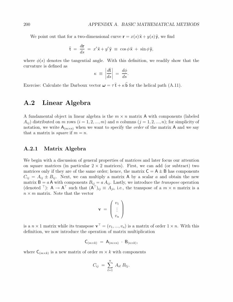
200 APPENDIX A. BASIC MATHEMATICAL METHODS
We point out that for a two-dimensional curve r = x(s) x + y(s) y, we find
t =dr
ds= x′ x + y′ y ≡ cos φ x + sinφ y,
where φ(s) denotes the tangential angle. With this definition, we readily show that thecurvature is defined as
κ ≡∣∣∣∣∣dt
ds
∣∣∣∣∣ =dφ
ds.
Exercise: Calculate the Darboux vector ω = τ t + κ b for the helical path (A.11).
A.2 Linear Algebra
A fundamental object in linear algebra is the m × n matrix A with components (labeledAij) distributed on m rows (i = 1, 2, ..., m) and n columns (j = 1, 2, ..., n); for simplicity ofnotation, we write A(m×n) when we want to specify the order of the matrix A and we saythat a matrix is square if m = n.
A.2.1 Matrix Algebra
We begin with a discussion of general properties of matrices and later focus our attentionon square matrices (in particular 2 × 2 matrices). First, we can add (or subtract) twomatrices only if they are of the same order; hence, the matrix C = A ± B has componentsCij = Aij ± Bij . Next, we can multiply a matrix A by a scalar a and obtain the newmatrix B = aA with components Bij = aAij. Lastly, we introduce the transpose operation(denoted >): A → A> such that (A>)ij ≡ Aji, i.e., the transpose of a m × n matrix is an ×m matrix. Note that the vector
v =
v1...vn
is a n× 1 matrix while its transpose v> = (v1, ..., vn) is a matrix of order 1× n. With thisdefinition, we now introduce the operation of matrix multiplication
C(m×k) = A(m×n) · B(n×k),
where C(m×k) is a new matrix of order m× k with components
Cij =n∑
`=1
Ai` B`j .
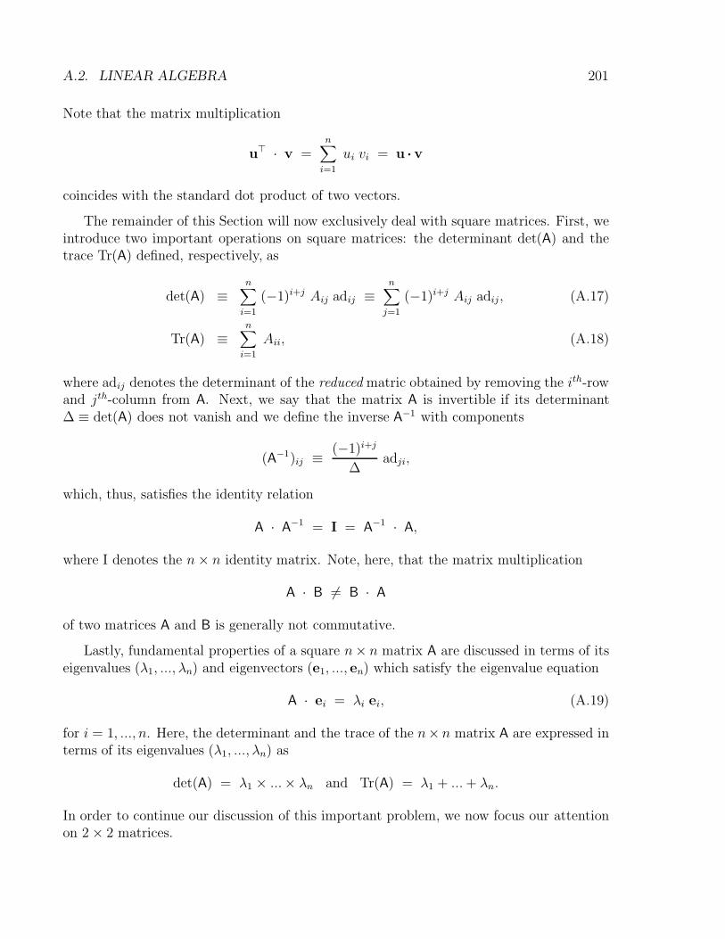
A.2. LINEAR ALGEBRA 201
Note that the matrix multiplication
u> · v =n∑
i=1
ui vi = u · v
coincides with the standard dot product of two vectors.
The remainder of this Section will now exclusively deal with square matrices. First, weintroduce two important operations on square matrices: the determinant det(A) and thetrace Tr(A) defined, respectively, as
det(A) ≡n∑
i=1
(−1)i+j Aij adij ≡n∑
j=1
(−1)i+j Aij adij, (A.17)
Tr(A) ≡n∑
i=1
Aii, (A.18)
where adij denotes the determinant of the reduced matric obtained by removing the ith-rowand jth-column from A. Next, we say that the matrix A is invertible if its determinant∆ ≡ det(A) does not vanish and we define the inverse A−1 with components
(A−1)ij ≡ (−1)i+j
∆adji,
which, thus, satisfies the identity relation
A · A−1 = I = A−1 · A,
where I denotes the n× n identity matrix. Note, here, that the matrix multiplication
A · B 6= B · A
of two matrices A and B is generally not commutative.
Lastly, fundamental properties of a square n× n matrix A are discussed in terms of itseigenvalues (λ1, ..., λn) and eigenvectors (e1, ..., en) which satisfy the eigenvalue equation
A · ei = λi ei, (A.19)
for i = 1, ..., n. Here, the determinant and the trace of the n× n matrix A are expressed interms of its eigenvalues (λ1, ..., λn) as
det(A) = λ1 × ...× λn and Tr(A) = λ1 + ...+ λn.
In order to continue our discussion of this important problem, we now focus our attentionon 2 × 2 matrices.
202 APPENDIX A. BASIC MATHEMATICAL METHODS
A.2.2 Eigenvalue analysis of a 2 × 2 matrix
Consider the 2 × 2 matrix
M =
(a bc d
)
, (A.20)
where (a, b, c, d) are arbitrary real (or complex) numbers and introduce the following twomatrix invariants:
∆ ≡ det(M) = a d− b c and σ ≡ Tr(M) = a + d, (A.21)
which denote the determinant and the trace of matrix M, respectively.
Eigenvalues of M
The eigenvalues λ and eigenvectors e of matrix M are defined by the eigenvalue equation
M · e = λe. (A.22)
This equation has nontrivial solutions only if the determinant of the matrix M−λ I vanishes(where I denotes the 2 × 2 identity matrix), which yields the characteristic quadraticpolynomial:
det(M − λ I) = (a− λ) (d − λ) − b c ≡ λ2 − σ λ + ∆, (A.23)
and the eigenvalues λ± are obtained as the roots of this characteristic polynomial:
λ± =σ
2±√σ2
4− ∆. (A.24)
Here, we note that the matrix invariants (σ,∆) are related to the eigenvalues λ±:
λ+ + λ− ≡ σ and λ+ · λ− ≡ ∆. (A.25)
Lastly, the eigenvalues are said to be degenerate if λ+ = λ− ≡ σ/2, i.e.,
∆ =σ2
4or b c = −
(a− d
2
)2
.
Eigenvectors of M
Next, the eigenvectors e± associated with the eigenvalues λ± are constructed from theeigenvalue equations M · e± = λ± e±, which yield the general solutions
e± ≡(
1µ±
)
ε±, (A.26)

A.2. LINEAR ALGEBRA 203
where ε± denotes an arbitrary constant and
µ± =λ± − a
b=
c
λ± − d. (A.27)
The normalization of the eigenvectors e± (|e±| = 1), for example, can be achieved bychoosing
ε± =1
√1 + (µ±)2
.
We note that the eigenvectors e± are not automatically orthogonal to each other (i.e., thedot product e+ · e− may not vanish). Indeed, we find
e+ · e− = ε+ ε− (1 + µ+ µ−), (A.28)
where
1 + µ+ µ− = 1 +1
b2(λ+ − a) (λ− − a) = 1 +
(a− d
2 b
)2
− 1
b2
(σ2
4− ∆
)
,
whose sign is indefinite. By using the Gram-Schmidt orthogonalization procedure, however,we may construct two orthogonal vectors (e1, e2):
e1 = α e+ + β e−
e2 = γ e+ + δ e−
, (A.29)
where the coefficients (α, β, γ, δ) are chosen to satisfy the orthogonalization conditione1 · e2 ≡ 0; it is important to note that the vectors (e1, e2) are not themselves eigenvectorsof the matrix M. For example, we may choose α = 1 = δ, β = 0, and
γ = −(
e+ · e−|e+|2
)
,
which corresponds to choosing e1 = e+ and constructing e2 as the component of e− thatis orthogonal to e+.
Lastly, we point out that any two-dimensional vector u may be decomposed in termsof the eigenvectors e±:
u =∑
i=±ui ei ≡
∑
i=±
(u · ei
|ei|2)
ei, (A.30)
where we assumed, here, that the eigenvectors are orthogonal to each other. Furthermore,the transformation M · u generates a new vector
v = M · u =∑
i=±ui M · ei ≡
∑
i=±vi ei,
where the components of v are vi ≡ ui λi.
204 APPENDIX A. BASIC MATHEMATICAL METHODS
Inverse of matrix M
The matrix (A.20) has an inverse, denoted M−1, if its determinant ∆ does not vanish. Inthis nonsingular case, we easily find
M−1 =1
∆
(d − b− c a
)
, (A.31)
so that M−1 · M = I = M · M−1. The determinant of M−1, denoted ∆′, is
∆′ =d a− b c
∆2≡ 1
∆=
1
λ+ · λ−,
while its trace, denoted σ′, is
σ′ =d+ a
∆≡ σ
∆=
1
λ++
1
λ−.
Hence, the eigenvalues of the inverse matrix (A.31) are
λ′± ≡ 1
λ±=
λ∓∆,
and its eigenvectors e± are identical to e± since
M · e± = λ± e± → e± = λ± M−1 · e± → M−1 · e± = λ−1± e± ≡ λ′± e±.
We note that once the inverse M−1 of a matrix M is known, then any inhomogeneous linearsystem of equations of the form M · u = v may be solved as u ≡ M−1 · v.
Special case I: Real Hermitian Matrix
A real matrix is said to be Hermitian if its transpose, denoted M> (i.e.,M>ij = Mji), satisfies
the identity M> = M, which requires that c = b in Eq. (A.20). In this case, the eigenvaluesare automatically real
λ± =
(a + d
2
)
±
√√√√(a− d
2
)2
+ b2,
and the associated eigenvectors (A.26), which are defined with
µ± = −(a− d
2b
)
±
√√√√1 +
(a− d
2
)2
,
are automatically orthogonal to each other (e+ · e− = 0) since µ+ µ− ≡ − 1.
A.2. LINEAR ALGEBRA 205
Special case II: Rotation Matrix
Another special matrix is given by the rotation matrix
R =
(cos θ sin θ
− sin θ cos θ
)
, (A.32)
with determinant det(R) = 1 and trace Tr(R) = 2 cos θ = eiθ + e−iθ. The rotation matrix(A.32) is said to be unitary since its transverse R> is equal to its inverse R−1 = R> (whichis possible only if its determinant is one).
The eigenvalues of the rotation matrix (A.32) are e±iθ and the eigenvectors are
e± =
(1± i
)
.
Note that the rotation matrix (A.32) can be written as R = exp(iθσ), where the matrix
σ =
(0 −ii 0
)
(also known as the Pauli spin matrix σ2) satisfies the properties σ2n = I and σ2n+1 = σ
and, thus, we find
exp(iθσ) =∞∑
n=0
(iθ)n
n!σn = cos θ I + i sin θ σ = R.
Note that the time derivative of the rotation matrix (A.32) satisfies the property
R−1 · R = i θ σ =
(0 θ
−θ 0
)
.
Lastly, we note that the rotation matrix (A.32) can be used to diagonalize a real Her-mitian matrix
M =
(a bb d
)
,
by constructing the new matrix
M = R>·M·R =
a+ (d − a) sin2 θ − b sin 2θ b cos 2θ − 1
2(d− a) sin 2θ
b cos 2θ − 12(d− a) sin 2θ d − (d − a) sin2 θ + b sin 2θ
. (A.33)
Next, by setting (assuming that d > a)
tan 2θ =2b
d − a→
cos 2θ = (d − a)/√σ2 − 4∆
sin 2θ = 2b/√σ2 − 4∆
,
206 APPENDIX A. BASIC MATHEMATICAL METHODS
where σ = a + d and ∆ = ad− b2 denote the trace and determinant of M, respectively, M
becomes a diagonal matrix
M =
(λ− 00 λ+
)
, (A.34)
where the diagonal components are
λ± =σ
2± 1
2
√σ2 − 4∆.
Note that the trace and determinant of M are the same as that of M, i.e., the trace and de-terminant of any real Hermitian matrix are invariant under the congruence transformation(A.33).
A.3 Important Integrals
The present Section summarizes the integral representation of trigonometric functions,which is used extensively in the integration by quadrature of several dynamical problems,e.g., light-ray propagation in a nonuniform medium, time-independent Hamiltonian sys-tems, and scattering problems. In addition, the basic theory of elliptic functions is in-troduced, so that the complete solution of some important dynamical problems (e.g., theforce-free evolution of an asymmetric top) can be presented.
A.3.1 Trigonometric Functions and Integrals
Trigonometric functions with period τ
Functions that are periodic, with period τ , are all related to trigonometric functions (withperiod 2π). Indeed, a periodic function f(t) can be represented in terms of a (Fourier)series involving cos(2πn t/τ ) and sin(2πn t/τ ), where n = 1, 2, ... represents the Fourierharmonic number.
Hence, the study of singly-periodic functions can focus its attention on the trigonometricfunctions sin z and cos z, defined in terms of the inverse formulas
z =∫ y
0
dx√1 − x2
= sin−1 y
=∫ 1
y
dx√1 − x2
= cos−1 y
Here, the period τ of the trigonometric functions sin z and cos z is defined as
1
4τ ≡
∫ 1
0
dx√1 − x2
=π
2
with the periodicity conditions: sin(z + n τ ) = sin z and cos(z + n τ ) = cos z.
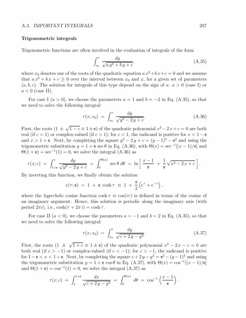
A.3. IMPORTANT INTEGRALS 207
Trigonometric integrals
Trigonometric functions are often involved in the evaluation of integrals of the form∫ x
x0
dy√a y2 + b y + c
, (A.35)
where x0 denotes one of the roots of the quadratic equation a x2+b x+c = 0 and we assumethat a x2 + b x + c ≥ 0 over the interval between x0 and x, for a given set of parameters(a, b, c). The solution for integrals of this type depend on the sign of a: a > 0 (case I) ora < 0 (case II).
For case I (a > 0), we choose the parameters a = 1 and b = −2 in Eq. (A.35), so thatwe need to solve the following integral:
τ (x; x0) =∫ x
x0
dy√y2 − 2 y + c
. (A.36)
First, the roots (1 ±√
1 − c ≡ 1± e) of the quadratic polynomial x2−2x+ c = 0 are bothreal (if c < 1) or complex-valued (if c > 1); for c < 1, the radicand is positive for x < 1− e
and x > 1 + e. Next, by completing the square y2 − 2 y + c = (y − 1)2 − e2 and using thetrigonometric substitution y = 1 + e sec θ in Eq. (A.36), with Θ(x) = sec−1[(x− 1)/e] andΘ(1 + e) = sec−1(1) = 0, we solve the integral (A.36) as
τ (x; c) =∫ x
1+e
dy√y2 − 2 y + c
=∫ Θ(x)
0sec θ dθ = ln
[x− 1
e+
1
e
√x2 − 2x+ c
].
By inverting this function, we finally obtain the solution
x(τ ; e) = 1 + e cosh τ ≡ 1 +e
2
(eτ + e−τ
),
where the hyperbolic cosine function cosh τ ≡ cos(iτ ) is defined in terms of the cosine ofan imaginary argument. Hence, this solution is periodic along the imaginary axis (withperiod 2πi), i.e., cosh(τ + 2π i) = cosh τ .
For case II (a < 0), we choose the parameters a = −1 and b = 2 in Eq. (A.35), so thatwe need to solve the following integral:
τ (x; x0) =∫ x
x0
dy√c+ 2 y − y2
. (A.37)
First, the roots (1 ±√
1 + c ≡ 1 ± e) of the quadratic polynomial x2 − 2x − c = 0 areboth real (if c > −1) or complex-valued (if c < −1); for c > −1, the radicand is positivefor 1− e < x < 1+ e. Next, by completing the square c+2 y− y2 = e2 − (y− 1)2 and usingthe trigonometric substitution y = 1 + e cos θ in Eq. (A.37), with Θ(x) = cos−1[(x− 1)/e]and Θ(1 + e) = cos−1(1) = 0, we solve the integral (A.37) as
τ (x; c) =∫ 1+e
x
dx√c+ 2 y − y2
=∫ Θ(x)
0dθ = cos−1
(x− 1
e
).
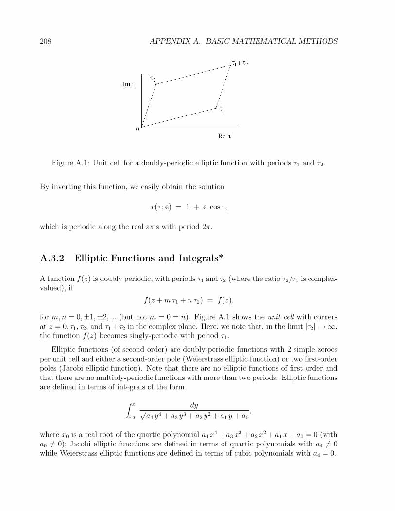
208 APPENDIX A. BASIC MATHEMATICAL METHODS
Figure A.1: Unit cell for a doubly-periodic elliptic function with periods τ1 and τ2.
By inverting this function, we easily obtain the solution
x(τ ; e) = 1 + e cos τ,
which is periodic along the real axis with period 2π.
A.3.2 Elliptic Functions and Integrals*
A function f(z) is doubly periodic, with periods τ1 and τ2 (where the ratio τ2/τ1 is complex-valued), if
f(z +mτ1 + n τ2) = f(z),
for m,n = 0,±1,±2, ... (but not m = 0 = n). Figure A.1 shows the unit cell with cornersat z = 0, τ1, τ2, and τ1 + τ2 in the complex plane. Here, we note that, in the limit |τ2| → ∞,the function f(z) becomes singly-periodic with period τ1.
Elliptic functions (of second order) are doubly-periodic functions with 2 simple zeroesper unit cell and either a second-order pole (Weierstrass elliptic function) or two first-orderpoles (Jacobi elliptic function). Note that there are no elliptic functions of first order andthat there are no multiply-periodic functions with more than two periods. Elliptic functionsare defined in terms of integrals of the form
∫ x
x0
dy√a4 y4 + a3 y3 + a2 y2 + a1 y + a0
,
where x0 is a real root of the quartic polynomial a4 x4 + a3 x
3 + a2 x2 + a1 x+ a0 = 0 (with
a0 6= 0); Jacobi elliptic functions are defined in terms of quartic polynomials with a4 6= 0while Weierstrass elliptic functions are defined in terms of cubic polynomials with a4 = 0.
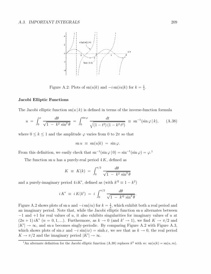
A.3. IMPORTANT INTEGRALS 209
Figure A.2: Plots of sn(u|k) and −i sn(iu|k) for k = 14.
Jacobi Elliptic Functions
The Jacobi elliptic function sn(u | k) is defined in terms of the inverse-function formula
u =∫ ϕ
0
dθ√1 − k2 sin2 θ
=∫ sinϕ
0
dt√
(1 − t2) (1 − k2 t2)≡ sn−1(sinϕ | k), (A.38)
where 0 ≤ k ≤ 1 and the amplitude ϕ varies from 0 to 2π so that
snu ≡ sn(u|k) = sinϕ.
From this definition, we easily check that sn−1(sinϕ | 0) = sin−1(sinϕ) = ϕ.1
The function sn u has a purely-real period 4K, defined as
K ≡ K(k) =∫ π/2
0
dθ√1 − k2 sin2 θ
and a purely-imaginary period 4 iK ′, defined as (with k′2 ≡ 1 − k2)
iK ′ ≡ iK(k′) = i∫ π/2
0
dθ√1 − k′2 sin2 θ
.
Figure A.2 shows plots of snu and −i sn(iu) for k = 14, which exhibit both a real period and
an imaginary period. Note that, while the Jacobi elliptic function sn u alternates between−1 and +1 for real values of u, it also exhibits singularities for imaginary values of u at(2n + 1) iK ′ (n = 0, 1, ...). Furthermore, as k → 0 (and k′ → 1), we find K → π/2 and|K ′| → ∞, and snu becomes singly-periodic. By comparing Figure A.2 with Figure A.3,which shows plots of sinx and −i sin(ix) = sinhx, we see that as k → 0, the real periodK → π/2 and the imaginary period |K ′| → ∞.
1An alternate definition for the Jacobi elliptic function (A.38) replaces k2 with m: sn(u|k) = sn(u, m).
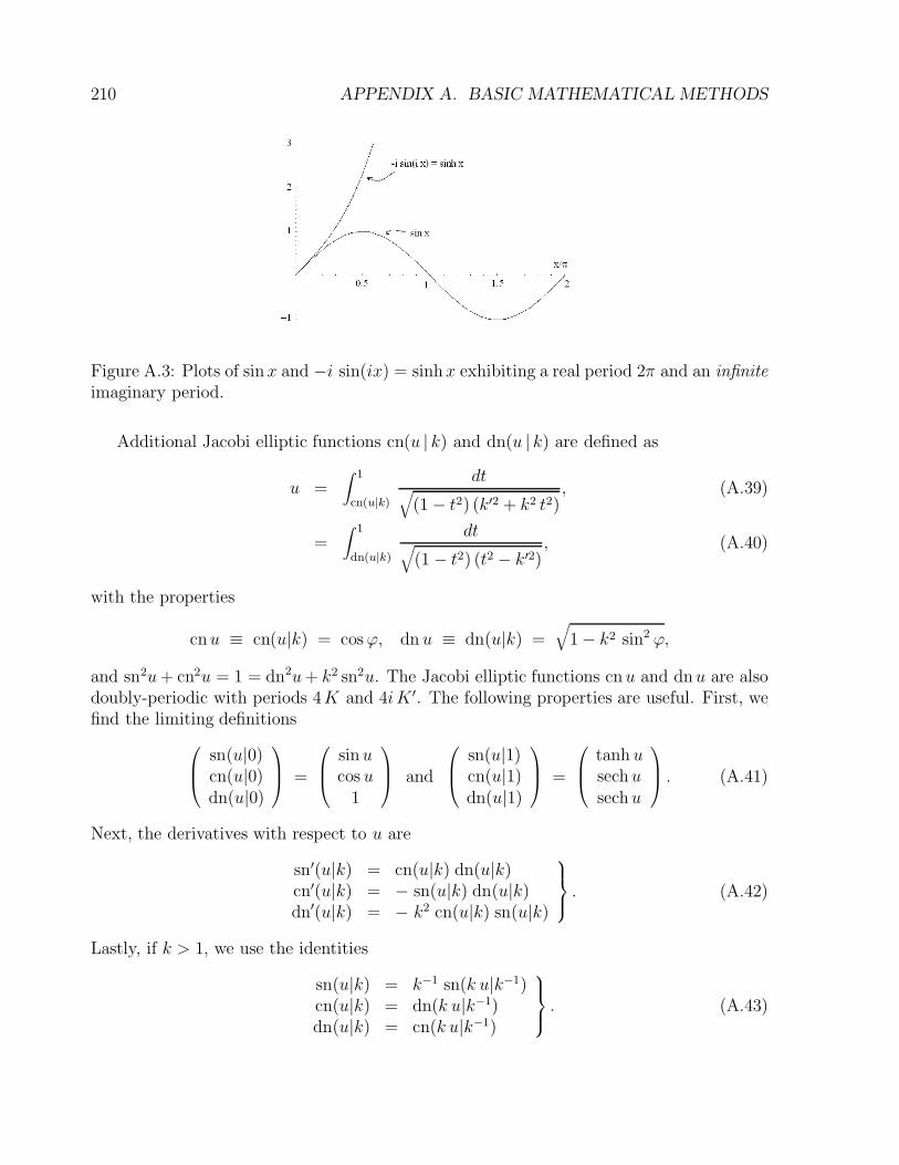
210 APPENDIX A. BASIC MATHEMATICAL METHODS
Figure A.3: Plots of sinx and −i sin(ix) = sinhx exhibiting a real period 2π and an infiniteimaginary period.
Additional Jacobi elliptic functions cn(u | k) and dn(u | k) are defined as
u =∫ 1
cn(u|k)
dt√
(1 − t2) (k′2 + k2 t2), (A.39)
=∫ 1
dn(u|k)
dt√
(1 − t2) (t2 − k′2), (A.40)
with the properties
cnu ≡ cn(u|k) = cosϕ, dn u ≡ dn(u|k) =√
1 − k2 sin2 ϕ,
and sn2u+ cn2u = 1 = dn2u+ k2 sn2u. The Jacobi elliptic functions cnu and dnu are alsodoubly-periodic with periods 4K and 4iK ′. The following properties are useful. First, wefind the limiting definitions
sn(u|0)cn(u|0)dn(u|0)
=
sinucos u
1
and
sn(u|1)cn(u|1)dn(u|1)
=
tanh usechusechu
. (A.41)
Next, the derivatives with respect to u are
sn′(u|k) = cn(u|k) dn(u|k)cn′(u|k) = − sn(u|k) dn(u|k)dn′(u|k) = − k2 cn(u|k) sn(u|k)
. (A.42)
Lastly, if k > 1, we use the identities
sn(u|k) = k−1 sn(k u|k−1)cn(u|k) = dn(k u|k−1)dn(u|k) = cn(k u|k−1)
. (A.43)
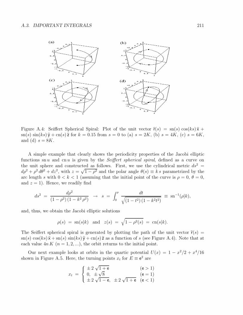
A.3. IMPORTANT INTEGRALS 211
Figure A.4: Seiffert Spherical Spiral: Plot of the unit vector r(s) = sn(s) cos(ks) x +sn(s) sin(ks) y + cn(s) z for k = 0.15 from s = 0 to (a) s = 2K, (b) s = 4K, (c) s = 6K,and (d) s = 8K.
A simple example that clearly shows the periodicity properties of the Jacobi ellipticfunctions snu and cnu is given by the Seiffert spherical spiral, defined as a curve onthe unit sphere and constructed as follows. First, we use the cylindrical metric ds2 =dρ2 + ρ2 dθ2 + dz2, with z =
√1 − ρ2 and the polar angle θ(s) ≡ k s parametrized by the
arc length s with 0 < k < 1 (assuming that the initial point of the curve is ρ = 0, θ = 0,and z = 1). Hence, we readily find
ds2 =dρ2
(1 − ρ2) (1 − k2 ρ2)→ s =
∫ ρ
0
dt√
(1 − t2) (1 − k2t2)≡ sn−1(ρ|k),
and, thus, we obtain the Jacobi elliptic solutions
ρ(s) = sn(s|k) and z(s) =√
1 − ρ2(s) = cn(s|k).
The Seiffert spherical spiral is generated by plotting the path of the unit vector r(s) =sn(s) cos(ks) x + sn(s) sin(ks) y + cn(s) z as a function of s (see Figure A.4). Note that ateach value 4nK (n = 1, 2, ...), the orbit returns to the initial point.
Our next example looks at orbits in the quartic potential U(x) = 1 − x2/2 + x4/16shown in Figure A.5. Here, the turning points xt for E ≡ e2 are
xt =
± 2√
1 + e (e > 1)
0, ±√
8 (e = 1)± 2
√1 − e, ± 2
√1 + e (e < 1)
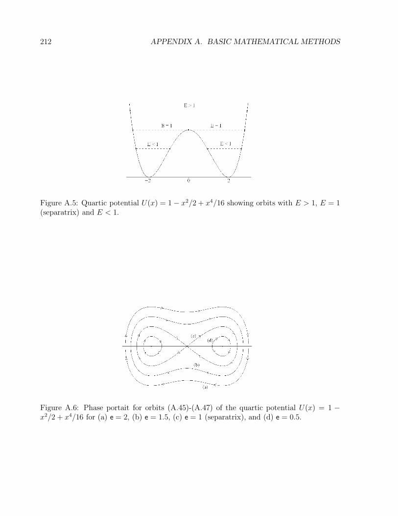
212 APPENDIX A. BASIC MATHEMATICAL METHODS
Figure A.5: Quartic potential U(x) = 1 − x2/2 + x4/16 showing orbits with E > 1, E = 1(separatrix) and E < 1.
Figure A.6: Phase portait for orbits (A.45)-(A.47) of the quartic potential U(x) = 1 −x2/2 + x4/16 for (a) e = 2, (b) e = 1.5, (c) e = 1 (separatrix), and (d) e = 0.5.
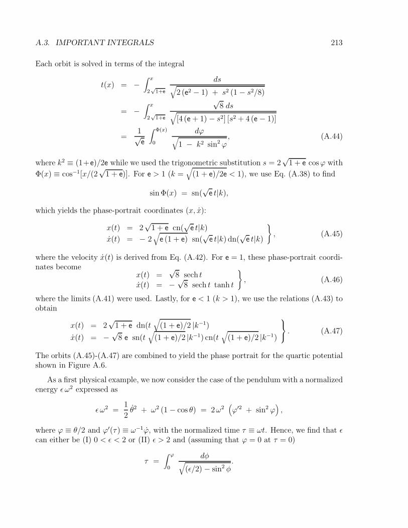
A.3. IMPORTANT INTEGRALS 213
Each orbit is solved in terms of the integral
t(x) = −∫ x
2√
1+e
ds√
2 (e2 − 1) + s2 (1 − s2/8)
= −∫ x
2√
1+e
√8 ds
√[4 (e + 1) − s2] [s2 + 4 (e − 1)]
=1√e
∫ Φ(x)
0
dϕ√
1 − k2 sin2 ϕ, (A.44)
where k2 ≡ (1+e)/2e while we used the trigonometric substitution s = 2√
1 + e cosϕ with
Φ(x) ≡ cos−1[x/(2√
1 + e)]. For e > 1 (k =√
(1 + e)/2e < 1), we use Eq. (A.38) to find
sinΦ(x) = sn(√
e t|k),
which yields the phase-portrait coordinates (x, x):
x(t) = 2√
1 + e cn(√
e t|k)x(t) = − 2
√e (1 + e) sn(
√e t|k) dn(
√e t|k)
, (A.45)
where the velocity x(t) is derived from Eq. (A.42). For e = 1, these phase-portrait coordi-nates become
x(t) =√
8 sech t
x(t) = −√
8 sech t tanh t
, (A.46)
where the limits (A.41) were used. Lastly, for e < 1 (k > 1), we use the relations (A.43) toobtain
x(t) = 2√
1 + e dn(t√
(1 + e)/2 |k−1)
x(t) = −√
8 e sn(t√
(1 + e)/2 |k−1) cn(t√
(1 + e)/2 |k−1)
. (A.47)
The orbits (A.45)-(A.47) are combined to yield the phase portrait for the quartic potentialshown in Figure A.6.
As a first physical example, we now consider the case of the pendulum with a normalizedenergy ε ω2 expressed as
ε ω2 =1
2θ2 + ω2 (1 − cos θ) = 2ω2
(ϕ′2 + sin2 ϕ
),
where ϕ ≡ θ/2 and ϕ′(τ ) ≡ ω−1ϕ, with the normalized time τ ≡ ωt. Hence, we find that εcan either be (I) 0 < ε < 2 or (II) ε > 2 and (assuming that ϕ = 0 at τ = 0)
τ =∫ ϕ
0
dφ√
(ε/2) − sin2 φ.
214 APPENDIX A. BASIC MATHEMATICAL METHODS
In case (I), where ε ≡ 2 sin2 α, we set sinφ = sinα sinχ and obtain (with k ≡ sinα)
τ =∫ sin−1(k−1 sinϕ)
0
dχ√
1 − k2 sin2 χ≡ sn−1(k−1 sinϕ | k).
Hence, the solution for case (I) is expressed in terms of the Jacobi elliptic function
ϕ(τ ) = sin−1 [ k sn(τ | k) ] ,
and in the limit k 1, we find the simple harmonic solution ϕ(τ ) = α sin τ , where αdenotes the amplitude of simple harmonic motion. In case (II), we have k−2 = 2/ε < 1 andobtain
τ = k−1∫ ϕ
0
dφ√
1 − k−2 sin2 φ≡ k−1 sn−1(sinϕ | k−1).
Hence, the solution for case (II) is expressed in terms of the Jacobi elliptic function
ϕ(τ ) = sin−1[sn(kτ | k−1)
].
Note that, in the limit k → 1, both solutions coincide with the separatrix solution (3.30),which is expressed in terms of singly-periodic trigonometric functions.
As a second physical example, we consider the Euler’s equations (7.25) for a force-freeasymmetric top (with I1 > I2 > I3), where conservation laws of kinetic energy (7.33) andangular momentum (7.34) lead to the following expressions
ω1(τ ) = −√√√√I2 (I2 − I3)
I1 (I1 − I3)Ω3
√1 − ν2(τ ), (A.48)
ω2(τ ) = Ω3 ν(τ ), (A.49)
ω3(τ ) =
√√√√I2 (I1 − I2)
I3 (I1 − I3)Ω1
√1 − k2 ν2(τ ), (A.50)
where Ω1 and Ω3 are defined in Eq. (7.38), with k2 = Ω23/Ω
21 ≤ 1, and τ = αΩ1 t, with α
defined in Eq. (7.37). When we substitute these expressions in the Euler equation (7.36)for ω2, we easily obtain
ν ′(τ ) =√
(1 − ν2) (1 − k2 ν2), (A.51)
which can now be integrated to yield
τ =∫ ν
0
ds√
(1 − s2) (1 − k2 s2)≡ sn−1(ν | k), (A.52)
orω2(τ ) = Ω3 sn(τ | k), (A.53)
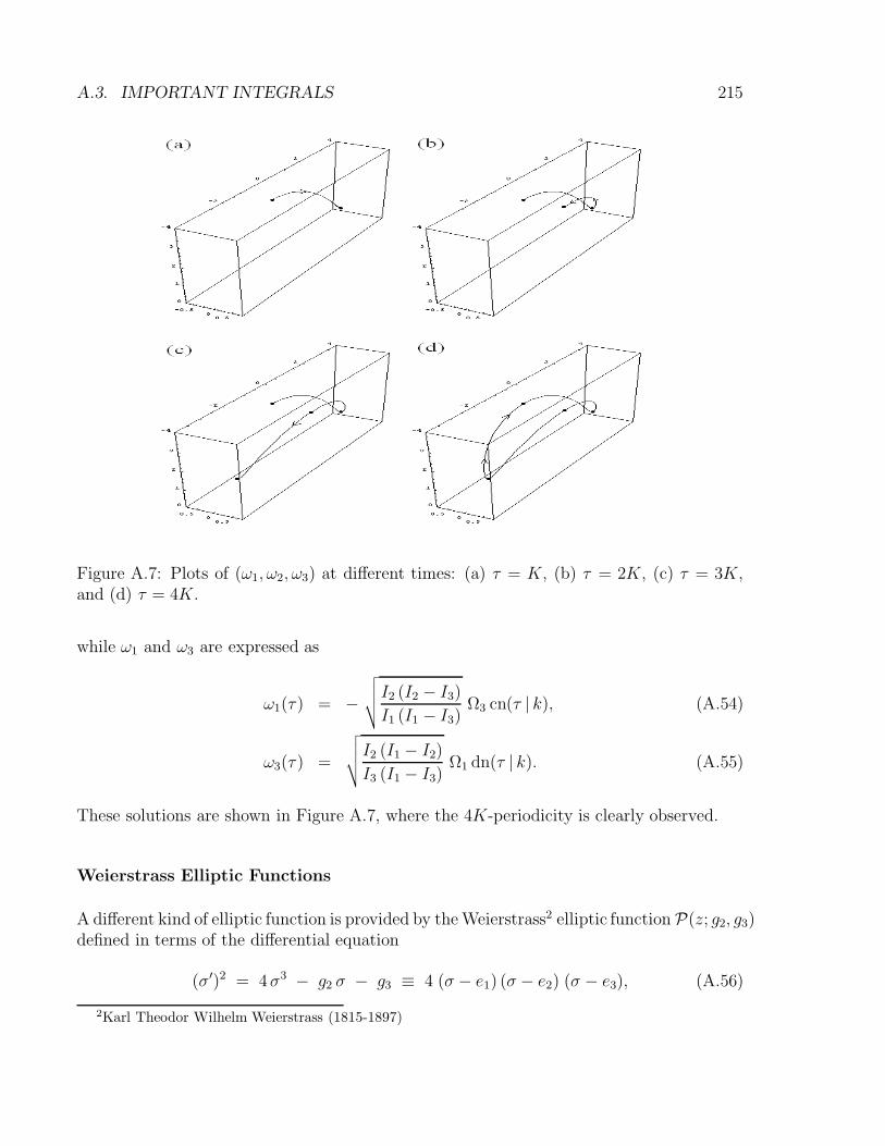
A.3. IMPORTANT INTEGRALS 215
Figure A.7: Plots of (ω1, ω2, ω3) at different times: (a) τ = K, (b) τ = 2K, (c) τ = 3K,and (d) τ = 4K.
while ω1 and ω3 are expressed as
ω1(τ ) = −√√√√I2 (I2 − I3)
I1 (I1 − I3)Ω3 cn(τ | k), (A.54)
ω3(τ ) =
√√√√I2 (I1 − I2)
I3 (I1 − I3)Ω1 dn(τ | k). (A.55)
These solutions are shown in Figure A.7, where the 4K-periodicity is clearly observed.
Weierstrass Elliptic Functions
A different kind of elliptic function is provided by the Weierstrass2 elliptic function P(z; g2, g3)defined in terms of the differential equation
(σ′)2 = 4σ3 − g2 σ − g3 ≡ 4 (σ − e1) (σ − e2) (σ − e3), (A.56)
2Karl Theodor Wilhelm Weierstrass (1815-1897)
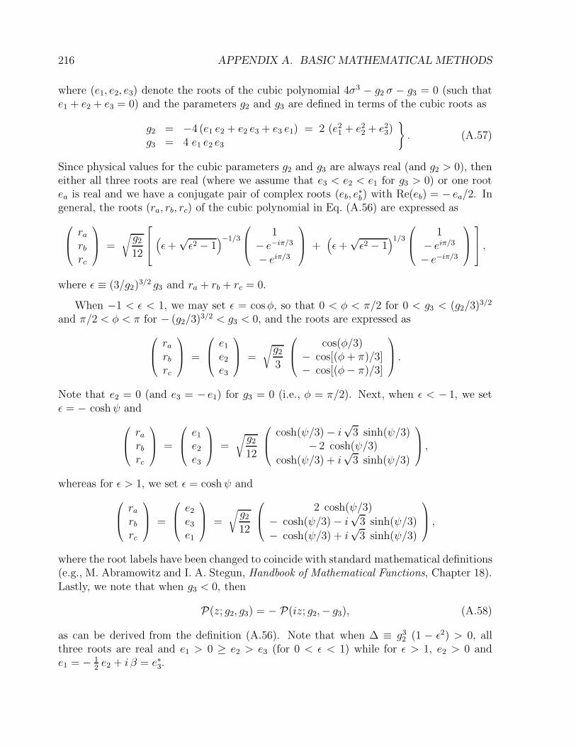
216 APPENDIX A. BASIC MATHEMATICAL METHODS
where (e1, e2, e3) denote the roots of the cubic polynomial 4σ3 − g2 σ − g3 = 0 (such thate1 + e2 + e3 = 0) and the parameters g2 and g3 are defined in terms of the cubic roots as
g2 = −4 (e1 e2 + e2 e3 + e3 e1) = 2 (e21 + e2
2 + e23)
g3 = 4 e1 e2 e3
. (A.57)
Since physical values for the cubic parameters g2 and g3 are always real (and g2 > 0), theneither all three roots are real (where we assume that e3 < e2 < e1 for g3 > 0) or one rootea is real and we have a conjugate pair of complex roots (eb, e
∗b) with Re(eb) = − ea/2. In
general, the roots (ra, rb, rc) of the cubic polynomial in Eq. (A.56) are expressed as
rarbrc
=
√g2
12
(ε+
√ε2 − 1
)−1/3
1
− e−iπ/3
− eiπ/3
+(ε+
√ε2 − 1
)1/3
1
− eiπ/3
− e−iπ/3
,
where ε ≡ (3/g2)3/2 g3 and ra + rb + rc = 0.
When −1 < ε < 1, we may set ε = cosφ, so that 0 < φ < π/2 for 0 < g3 < (g2/3)3/2
and π/2 < φ < π for − (g2/3)3/2 < g3 < 0, and the roots are expressed as
rarbrc
=
e1
e2
e3
=
√g2
3
cos(φ/3)
− cos[(φ+ π)/3]− cos[(φ− π)/3]
.
Note that e2 = 0 (and e3 = − e1) for g3 = 0 (i.e., φ = π/2). Next, when ε < − 1, we setε = − coshψ and
rarbrc
=
e1
e2
e3
=√g2
12
cosh(ψ/3) − i
√3 sinh(ψ/3)
− 2 cosh(ψ/3)
cosh(ψ/3) + i√
3 sinh(ψ/3)
,
whereas for ε > 1, we set ε = coshψ and
rarbrc
=
e2
e3
e1
=
√g2
12
2 cosh(ψ/3)
− cosh(ψ/3) − i√
3 sinh(ψ/3)
− cosh(ψ/3) + i√
3 sinh(ψ/3)
,
where the root labels have been changed to coincide with standard mathematical definitions(e.g., M. Abramowitz and I. A. Stegun, Handbook of Mathematical Functions, Chapter 18).Lastly, we note that when g3 < 0, then
P(z; g2, g3) = − P(iz; g2,− g3), (A.58)
as can be derived from the definition (A.56). Note that when ∆ ≡ g32 (1 − ε2) > 0, all
three roots are real and e1 > 0 ≥ e2 > e3 (for 0 < ε < 1) while for ε > 1, e2 > 0 ande1 = − 1
2e2 + i β = e∗3.
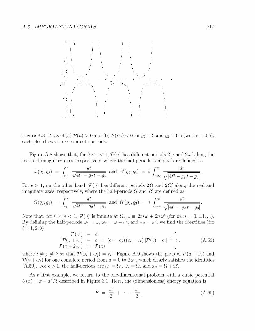
A.3. IMPORTANT INTEGRALS 217
Figure A.8: Plots of (a) P(u) > 0 and (b) P(i u) < 0 for g2 = 3 and g3 = 0.5 (with ε = 0.5);each plot shows three complete periods.
Figure A.8 shows that, for 0 < ε < 1, P(u) has different periods 2ω and 2ω′ along thereal and imaginary axes, respectively, where the half-periods ω and ω′ are defined as
ω(g2, g3) =∫ ∞
e1
dt√4t3 − g2 t− g3
and ω′(g2, g3) = i∫ e3
−∞
dt√|4t3 − g2 t− g3|
.
For ε > 1, on the other hand, P(u) has different periods 2Ω and 2Ω′ along the real andimaginary axes, respectively, where the half-periods Ω and Ω′ are defined as
Ω(g2, g3) =∫ ∞
e2
dt√4t3 − g2 t− g3
and Ω′(g2, g3) = i∫ e2
−∞
dt√|4t3 − g2 t− g3|
.
Note that, for 0 < ε < 1, P(u) is infinite at Ωm,n ≡ 2mω + 2nω′ (for m,n = 0,±1, ...).By defining the half-periods ω1 = ω, ω2 = ω + ω′, and ω3 = ω′, we find the identities (fori = 1, 2, 3)
P(ωi) = eiP(z + ωi) = ei + (ei − ej) (ei − ek) [P(z) − ei]
−1
P(z + 2ωi) = P(z)
, (A.59)
where i 6= j 6= k so that P(ωi + ωj) = ek. Figure A.9 shows the plots of P(u + ω2) andP(u+ ω3) for one complete period from u = 0 to 2ω1, which clearly satisfies the identities(A.59). For ε > 1, the half-periods are ω1 = Ω′, ω2 = Ω, and ω3 = Ω + Ω′.
As a first example, we return to the one-dimensional problem with a cubic potentialU(x) = x− x3/3 described in Figure 3.1. Here, the (dimensionless) energy equation is
E =x2
2+ x − x3
3, (A.60)
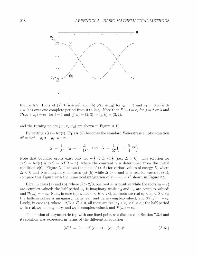
218 APPENDIX A. BASIC MATHEMATICAL METHODS
Figure A.9: Plots of (a) P(u + ω2) and (b) P(u + ω3) for g2 = 3 and g3 = 0.5 (withε = 0.5) over one complete period from 0 to 2ω1. Note that P(ωj) = ej for j = 2 or 3 andP(ωi + ωj) = ek, for i = 1 and (j, k) = (2, 3) or (j, k) = (3, 2).
and the turning points (x1, x2, x3) are shown in Figure A.10.
By writing x(t) = 6σ(t), Eq. (A.60) becomes the standard Weierstrass elliptic equationσ2 = 4σ3 − g2 σ − g3, where
g2 =1
3, g3 = − E
18, and ∆ =
1
27
(1 − 9
4E2).
Note that bounded orbits exist only for − 23< E < 2
3(i.e., ∆ > 0). The solution for
x(t) = 6σ(t) is x(t) = 6P(t + γ), where the constant γ is determined from the initialcondition x(0). Figure A.11 shows the plots of (x, x) for various values of energy E, where∆ < 0 and φ is imaginary for cases (a)-(b) while ∆ > 0 and φ is real for cases (c)-(d);compare this Figure with the numerical integration of x = −1 + x2 shown in Figure 3.2.
Here, in cases (a) and (b), where E > 2/3, one root e1 is positive while the roots e2 = e∗3are complex-valued; the half-period ω1 is imaginary while ω2 and ω3 are complex-valued;and P(ωi) = − ei. Next, in case (c), where 0 < E < 2/3, all roots are real e3 < e2 < 0 < e1;the half-period ω1 is imaginary, ω3 is real, and ω2 is complex-valued; and P(ωi) = − ei.Lastly, in case (d), where −2/3 < E < 0, all roots are real e3 < e2 < 0 < e1; the half-periodω1 is real, ω3 is imaginary, and ω2 is complex-valued; and P(ωi) = ei.
The motion of a symmetric top with one fixed point was discussed in Section 7.3.4 andits solution was expressed in terms of the differential equation
(u′)2 = (1 − u2)(ε− u) − (α− β u)2, (A.61)
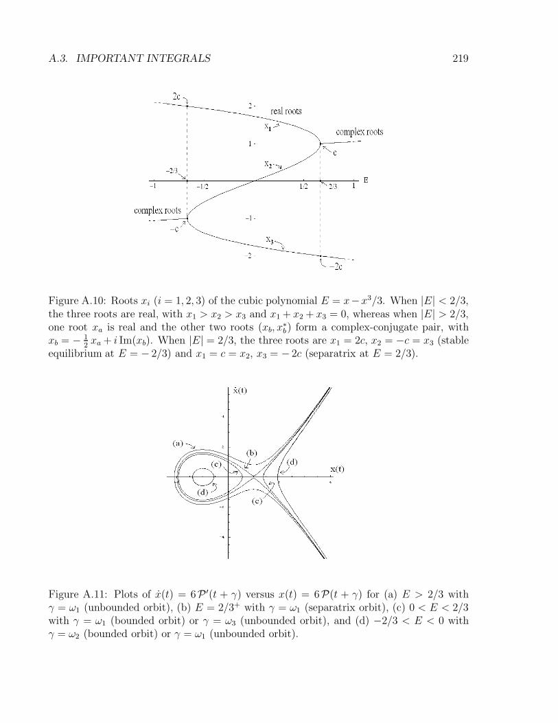
A.3. IMPORTANT INTEGRALS 219
Figure A.10: Roots xi (i = 1, 2, 3) of the cubic polynomial E = x−x3/3. When |E| < 2/3,the three roots are real, with x1 > x2 > x3 and x1 + x2 + x3 = 0, whereas when |E| > 2/3,one root xa is real and the other two roots (xb, x
∗b) form a complex-conjugate pair, with
xb = − 12xa + i Im(xb). When |E| = 2/3, the three roots are x1 = 2c, x2 = −c = x3 (stable
equilibrium at E = − 2/3) and x1 = c = x2, x3 = − 2c (separatrix at E = 2/3).
Figure A.11: Plots of x(t) = 6P ′(t + γ) versus x(t) = 6P(t + γ) for (a) E > 2/3 withγ = ω1 (unbounded orbit), (b) E = 2/3+ with γ = ω1 (separatrix orbit), (c) 0 < E < 2/3with γ = ω1 (bounded orbit) or γ = ω3 (unbounded orbit), and (d) −2/3 < E < 0 withγ = ω2 (bounded orbit) or γ = ω1 (unbounded orbit).

220 APPENDIX A. BASIC MATHEMATICAL METHODS
where the constants (ε, α, β) were defined in Section 7.3.4. By using the change of integra-tion variable u = 4σ + γ, where γ = (ε+ β2)/3, the differential equation (A.61) becomesthe standard differential equation (A.56) for the Weierstrass elliptic function, with
g2 =1
4
[(1 − 2αβ) + 3γ2
],
g3 =1
16
[α2 − ε + γ (1 − 2αβ) + 2γ3
].
Hence, the solution is expressed in terms of the Weierstrass elliptic function as
u(τ ) = 4P(τ + δ) + γ,
where δ is determined initial conditions, and we denote the three roots e1 > e2 > e3 of thecubic polynomial 4σ3−g2 σ−g3 = 0. Assuming that 4 e1 +γ > 1, then at τ = 0, we chooseu(0) = u1 = 4 e3 + γ so that δ ≡ ω3 and, hence, at τ = ω1, we find
u(ω1) = 4P(ω1 + ω3) + γ = 4 e2 + γ = u2.
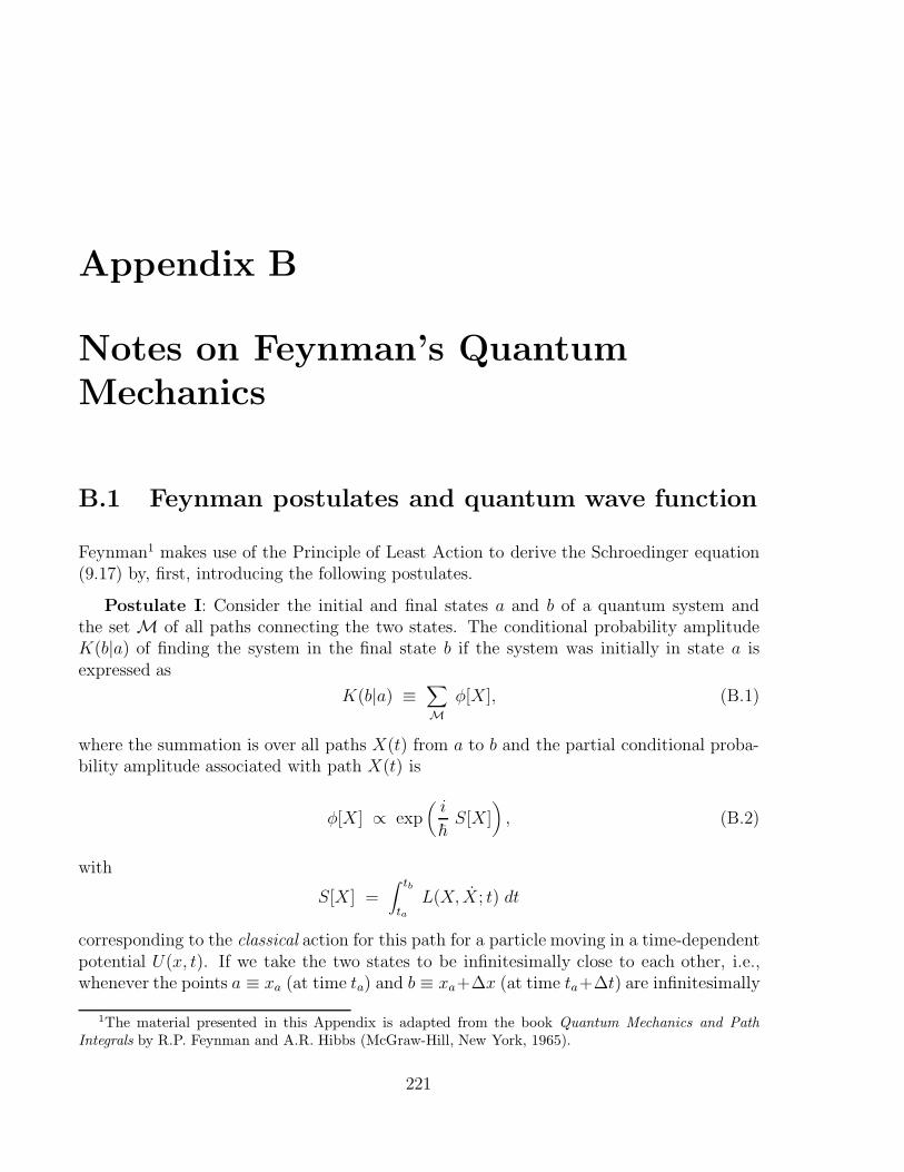
Appendix B
Notes on Feynman’s Quantum
Mechanics
B.1 Feynman postulates and quantum wave function
Feynman1 makes use of the Principle of Least Action to derive the Schroedinger equation(9.17) by, first, introducing the following postulates.
Postulate I: Consider the initial and final states a and b of a quantum system andthe set M of all paths connecting the two states. The conditional probability amplitudeK(b|a) of finding the system in the final state b if the system was initially in state a isexpressed as
K(b|a) ≡∑
Mφ[X], (B.1)
where the summation is over all paths X(t) from a to b and the partial conditional proba-bility amplitude associated with path X(t) is
φ[X] ∝ exp(i
hS[X]
), (B.2)
with
S[X] =∫ tb
taL(X, X ; t) dt
corresponding to the classical action for this path for a particle moving in a time-dependentpotential U(x, t). If we take the two states to be infinitesimally close to each other, i.e.,whenever the points a ≡ xa (at time ta) and b ≡ xa+∆x (at time ta+∆t) are infinitesimally
1The material presented in this Appendix is adapted from the book Quantum Mechanics and Path
Integrals by R.P. Feynman and A.R. Hibbs (McGraw-Hill, New York, 1965).
221
222 APPENDIX B. NOTES ON FEYNMAN’S QUANTUM MECHANICS
close, Eqs. (B.1)-(B.2) yield
K(xa + ∆x, ta + ∆t|xa, ta) =1
Aexp
i
h
[m(∆x)2
2∆t− ∆t U
(xa +
∆x
2, ta +
∆t
2
) ]
, (B.3)
where A is a normalization constant and the classical action integral
S[x] =∫ ta+∆t
ta
m2
(dx
dt
)2
− U(x, t)
dt =m(∆x)2
2∆t− U
(xa +
∆x
2, ta +
∆t
2
)∆t
is a function of ∆x and ∆t as well as the initial space-time point (xa, ta); here, the potentialenergy U is evaluated at the mid-point between xa and xb at a time ta + ∆t/2.
Postulate I provides the appropriate explanation for the mystery behind the Principleof Least Action (“act locally, think globally”). Indeed, in the classical limit (h → 0), wefind that the variations δX around the paths X(t) which are far away from the physicalpath x(t) yield changes δS for which δS/h is large. Consequently, such contributions tendto average out to zero because of the corresponding wild oscillations in φ[X]. On the otherhand, for variations δX near the physical path x(t), we get δS ∼ 0 (to first order) and,consequently, paths X(t) for which S[X] is within h of Scl will contribute strongly. Theresulting effect is that only paths in the neighborhood of the physical path x(t) have anonvanishing probability amplitude. In the strict limit h → 0, the only such path with anonvanishing probability amplitude is the physical path.
Postulate II: The quantum wave function ψ(x, t) is defined as the probability ampli-tude for the particle to be at the location x at time t, i.e., ψ(x, t) ≡ K(x, t|•), where weare not interested in the previous history of the particle (its previous location is denotedby •) but only on its future time evolution. The Second Postulate states that the integralequation relating the wave function ψ(x2, t2) to the wave function ψ(x1, t1) is given as
ψ(x2, t2) ≡∫ ∞
−∞dx1 K(x2, t2|x1, t1) ψ(x1, t1). (B.4)
If we set in Eq. (B.4): t1 = t and t2 = t+ ε, x2 = x and x1 = x+ η, then for small enoughvalues of ε, the conditional probability amplitude (B.3) can be used in (B.4) to yield
ψ(x, t+ ε) ≡∫ ∞
−∞dη K(x, t+ ε|x+ η, t) ψ(x+ η, t) (B.5)
=∫ ∞
−∞
dη
Aexp
[i
h
(mη2
2ε− ε U(x+ η/2, t+ ε/2)
) ]
ψ(x+ η, t),
where a time-dependent potential U(x, t) is considered.
B.2. DERIVATION OF THE SCHROEDINGER EQUATION 223
B.2 Derivation of the Schroedinger equation
We will now derive the Schroedinger equation by expanding both sides of Eq. (B.5), up tofirst order in ε (and neglect all higher powers). First, on the left side of Eq. (B.5), we have
ψ(x, t+ ε) = ψ(x, t) + ε∂ψ(x, t)
∂t. (B.6)
Next, on the right side of Eq. (B.5), we note that the exponential
exp
[ (im
2h
)η2
ε
]
oscillates wildly as ε → 0 for all values of η except those for which mη2/(2hε) ∼ 1. We,therefore, conclude that the contribution from the integral in Eq. (B.5) will come fromvalues η = O(ε1/2) and, consequently, we may expand the remaining functions appearingon the right side of Eq. (B.5) up to η2. Thus, we may write
ψ(x+ η, t) = ψ(x, t) + η∂ψ(x, t)
∂x+
η2
2
∂2ψ(x, t)
∂x2,
while
exp[− iε
hU(x+ η/2, t+ ε/2)
]= 1 − iε
hU(x, t).
Expanding the right side of Eq. (B.5) to first order in ε, therefore, yields
[1 − iε
hU(x, t)
]ψ(x, t) +
(I1I0
)∂ψ(x, t)
∂x+(I22 I0
)∂2ψ(x, t)
∂x2, (B.7)
where A = I0 and
In ≡∫ ∞
−∞dη ηn e−aη
2
, a ≡ m
2ihε
with I0 =√π/a, I1 = 0, and I2 = 1/2a = (ih/m) ε.
Lastly, we find that the terms of first order in ε in Eqs. (B.6) and (B.7) must be equal,and we obtain
∂ψ(x, t)
∂t= − i
hU(x, t) ψ(x, t) +
ih
2m
∂2ψ(x, t)
∂x2,
or
ih∂ψ(x, t)
∂t= − h2
2m
∂2ψ(x, t)
∂x2+ U(x, t) ψ(x, t). (B.8)
This equation is known as the Schroedinger equation and it describes the time evolutionof the wave function ψ(x, t).