Lagrangian Continuum Mechanics Variables for General Nonlinear

Contents:

Textbook:

Examples:

Topic 3

LagrangianContinuumMechanicsVariables forGeneral NonlinearAnalysis

• The principle of virtual work in terms of the 2nd Piola-Kirchhoff stress and Green-Lagrange strain tensors

• Deformation gradient tensor

• Physical interpretation of the deformation gradient

• Change of mass density

• Polar decomposition of deformation gradient

• Green-Lagrange strain tensor

• Second Piola-Kirchhoff stress tensor

• Important properties of the Green-Lagrange strain and2nd Piola-Kirchhoff stress tensors

• Physical explanations of continuum mechanics variables

• Examples demonstrating the properties of the continuummechanics variables

Sections 6.2.1, 6.2.2

6.5,6.6,6.7,6.8,6.10,6.11,6.12,6.13,6.14

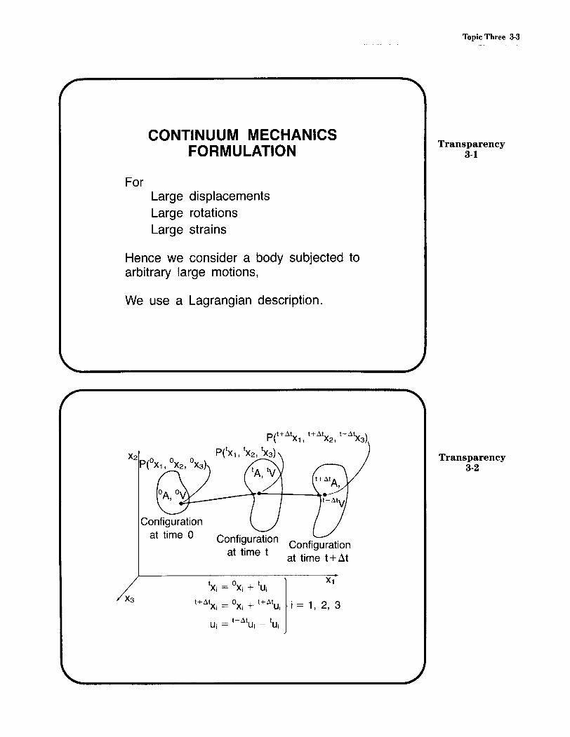
CONTINUUM MECHANICSFORMULATION

ForLarge displacementsLarge rotationsLarge strains

Hence we consider a body subjected toarbitrary large motions,

We use a Lagrangian description.

Topic Three 3-3

Transparency3-1

Configurationat time 0

PC+~'X1, t+~'X2, '+~'X3)

PCX1, 'X2, 'X3)

Confi~uration Configurationat time t at time t + ~t

Transparency3-2

'Xi = °Xi + lUi I X1

t+~'x· = ox· + t+~'u· i = 1 2 3I I I "

U· - t+~'u· - 'u·1- I I

3-4 Lagrangian Continuum Mechanics Variables

Transparency3-3

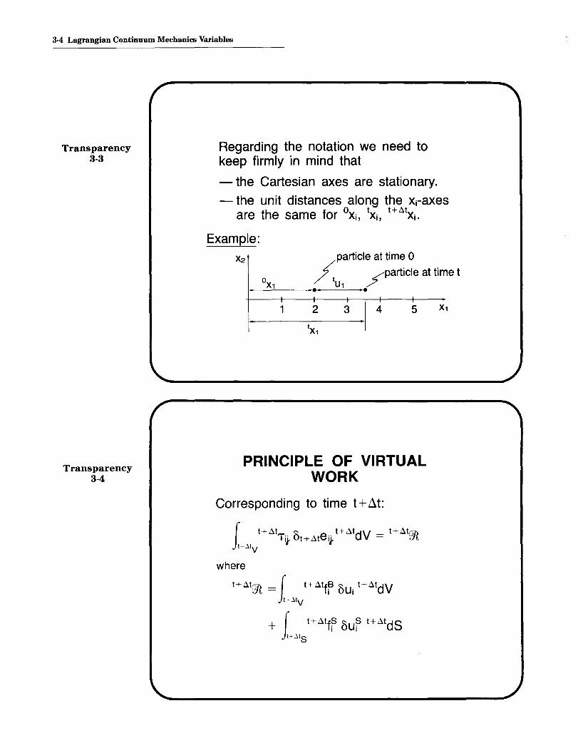
Regarding the notation we need tokeep firmly in mind that

- the Cartesian axes are stationary.

- the unit distances along the Xi-axesare the same for °Xi, tXi , t+ ~tXi.

Example:particle at time 0

0X1 /U1 /particle at time t1----'---·.· ...

1 2 3 4 5

Transparency3-4

PRINCIPLE OF VIRTUALWORK

Corresponding to time t+dt:

I t+~tlT'.. ~ e·· t+~tdV - t+~t(flllit Ut+~t It -;nt+.ltv

where

t+~tffi = r t+~tfF OUi t+~tdV)t+.ltv

+ r t+~tfr OUr t+~tdS)t+.lts

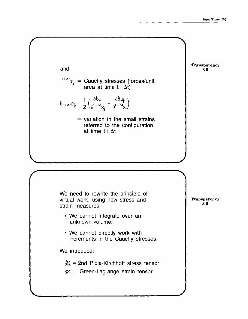
t+Atl'T"..I 'I'

and

Cauchy stresses (forces/unitarea at time t +Llt)

1 ( aOUi aou} )ot+Atei} = 2 at+Atx} + at+Atxi

variation in the small strainsreferred to the configurationat time t +Llt

We need to rewrite the principle ofvirtual work, using new stress andstrain measures:

• We cannot integrate over anunknown volume.

• We cannot directly work withincrements in the Cauchy stresses.

We introduce:

cis = 2nd Piola-Kirchhoff stress tensor

6E = Green-Lagrange strain tensor

Topic Three 3-5

Transparency3·5

Transparency3·6


Transparency3-7

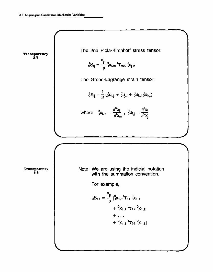
The 2nd Piola-Kirchhoff stress tensor:

at8 POt aa i} = -t tXi,m Tmn tX},n

P

The Green-Lagrange strain tensor:

t 1 (t t t t )OE" = - aU·" + au.. + aUk" aUk"yo 2 I,t ~I ,I ,t

where

Transparency3-8

Note: We are using the indicial notationwith the summation convention.

For example,

at Pro t a0811 = -t tX1,1 Tn tX1,1

Pa t a+ tX1 ,1 T 12 tX1 ,2

+ ...+ ~X1,3 tT33 ~X1,3]

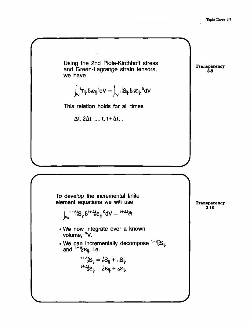
Using the 2nd Piola-Kirchhoff stressand Green-Lagrange strain tensors,we have

This relation holds for all times

at, 2at, ... , t, t+at, ...

To develop the incremental finiteelement equations we will use

~vt+~JSt 8t+~JEt °dV = t+~~

• We now integrate over a knownvolume, °V.

• We can incrementally decompose t+~JStd t+~t .

an oEt, I.e.

t+~ts ts So ~=o iJ-+O iJ-t+~t t

OEiJ- = oE~ + oE~

Topic Three 3·7

Transparency3-9

Transparency3-10


Transparency3-11

Transparency3-12

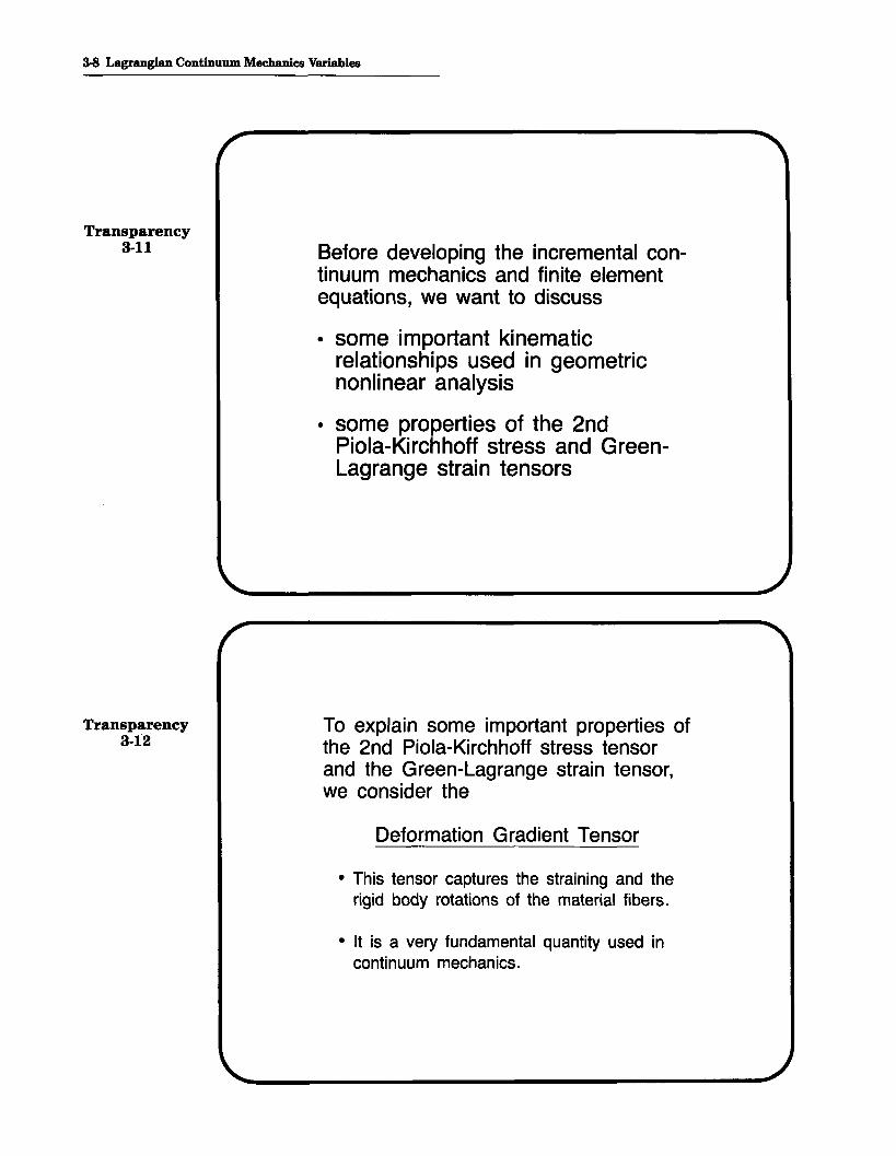
Before developing the incremental continuum mechanics and finite elementequations, we want to discuss

• some important kinematicrelationships used in geometricnonlinear analysis

• some properties of the 2ndPiola-Kirchhoff stress and GreenLagrange strain tensors

To explain some important properties ofthe 2nd Piola-Kirchhoff stress tensorand the Green-Lagrange strain tensor,we consider the

Deformation Gradient Tensor

• This tensor captures the straining and therigid body rotations of the material fibers.

• It is a very fundamental quantity used incontinuum mechanics.

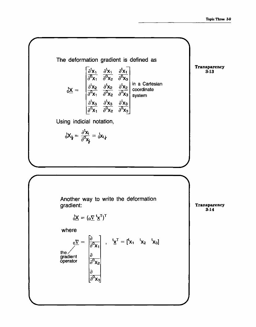
The deformation gradient is defined as

atx1aOx1

atx2

aOX1

atXaaOX1

atx1aOX2

atX2aOX2

atXaaOX2

atx1aOXa

atx2aOXa

atXaaOXa

in a Cartesiancoordinatesystem

Topic Three 3-9

Transparency3-13

Using indicial notation,

Another way to write the deformationgradient:

Jx = (oVJt~T)T

where

Transparency3-14

oV =

the/gradientoperator


Transparency3-15

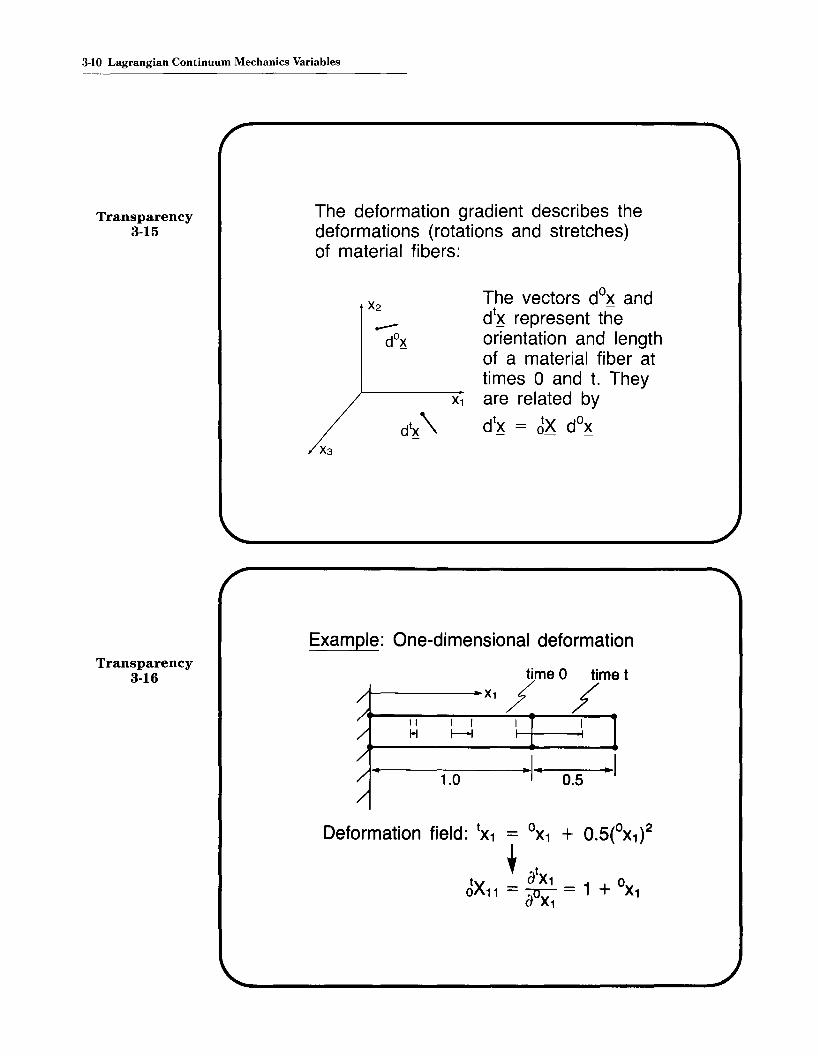
The deformation gradient describes thedeformations (rotations and stretches)of material fibers:

The vectors dOx anddt~ represent theorientation and lengthof a material fiber attimes 0 and t. Theyare related bydtx JX dOx

Transparency3-16

Example: One-dimensional deformation

time 0 time t

X1/ /'11H

...I....-------al.....--._.. 11.0 0.5

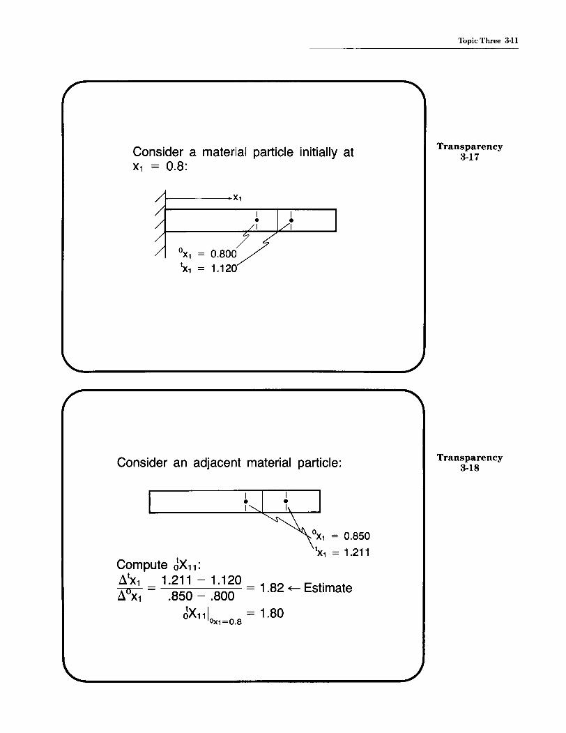
Consider a material particle initially atX1 = 0.8:

f------X1

°X1 = 0.8001<1 = 1.120

Consider an adjacent material particle:

Topic Three 3-11

Transparency3-17

Transparency3-18

I•I

Compute Jx11 :

d tx1 1.211 - 1.120d OX1 = .850 - .800 = 1.82 ~ Estimate

JX11 lo = 1.80x1=O.8


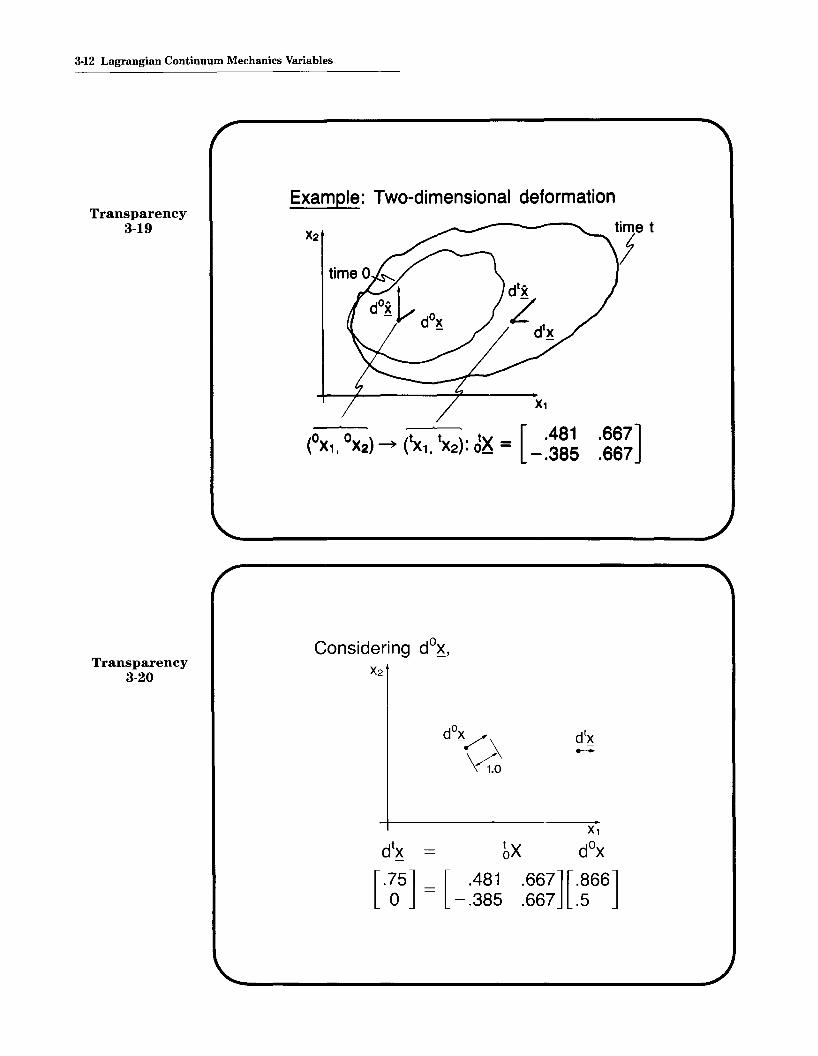
Exam~: Two-dimensional deformationTransparency

3-19

Transparency3-20

(0 0) (t t ). tx [ .481X1, X2 ~ X1. X2 ·0_ = -.385

Considering dO~,

X2

time t

f

.667]

.667

X1

dt~ = hx dO~

[ .75] = [ .481 .667][.866]o - .385 .667 .5

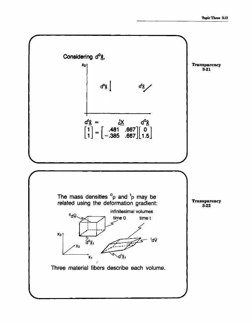
Considering cf!.X2

dtx = tx cfx_ 0_ _

[1] [.481 .667][ 0]1 = -.385 .667 1.5

The mass densittes 0p and tp may berelated using the deformation gradient:

infinitesimal volumes

time 0 time t

//:::;;:;Ls- tdV

~~dt!l

Three material fibers describe each volume.

'Ibpic Three 3-13

Transparency3-21

Transparency3-22


Transparency3-23

Transparency3-24

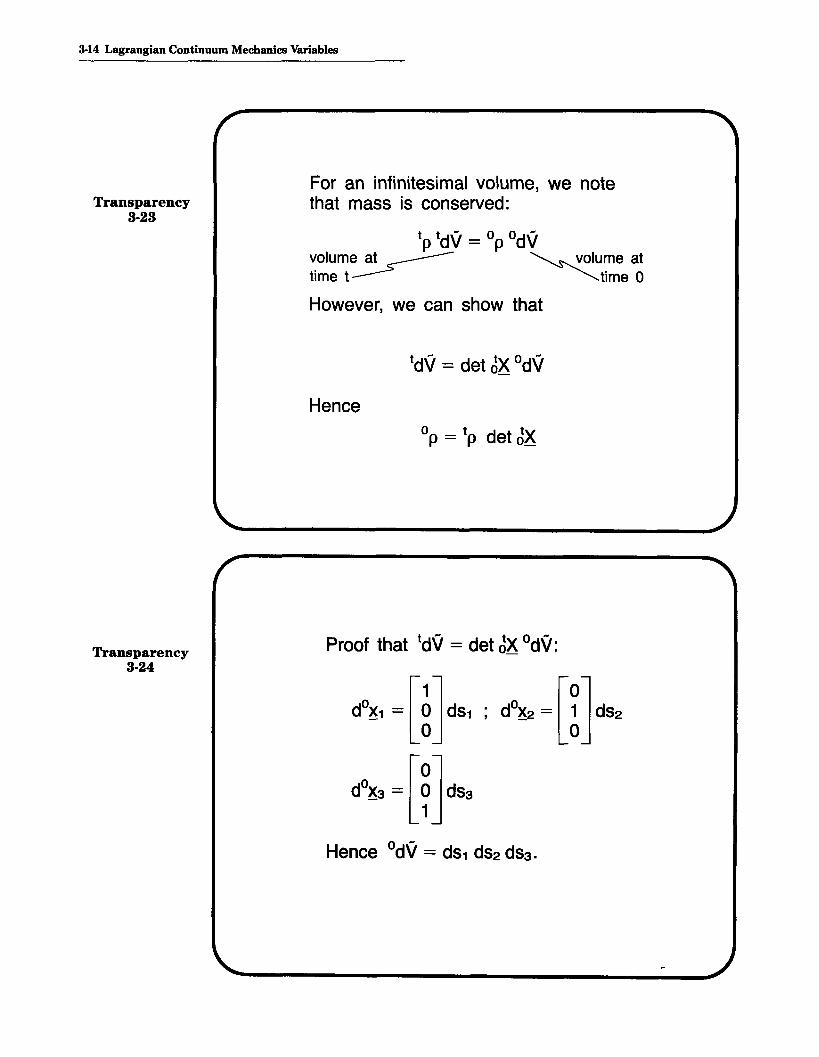
For an infinitesimal volume, we notethat mass is conserved:

tp tdV = 0p 0dVvolume at .----:--- ~~volume attime t~ - ~time 0

However, we can show that

Hence

Proof that tdV = det Jx °dV:

dO~1 =[g}S1 ; dO~ =[!}S2

dO~=[~}S3° -Hence dV = dS1 dS2 ds3 •

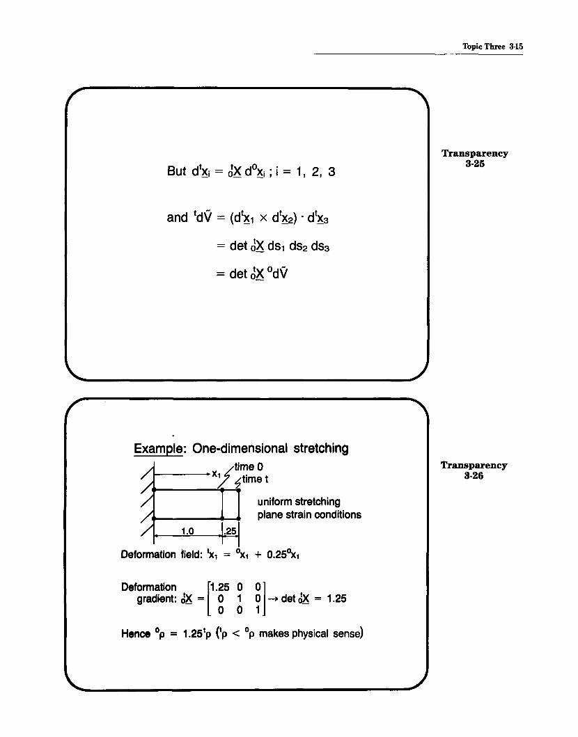
and tdV = (dt~1 X dt~2) . dt~3

= det Jx dS1 dS2 dS3

= det Jx °dV

Example: One-dimensional stretching

/1 ~timeO

,/, x:r ~time t

/ uniform stretching// plane strain conditions

1.0 .25

Deformation field: 'x, = ox, + O.250x,

Deformation [1.25 0 01gradient: J~ = 0 1 0 -+ det J~ = 1.25

o 0 1

Hence 0p = 1.25tp (tp < 0p makes physical sense)

'""""""-----------------",

Topic Three 3-15

Transparency3-25

Transparency3-26


Transparency3-27

Transparency3-28

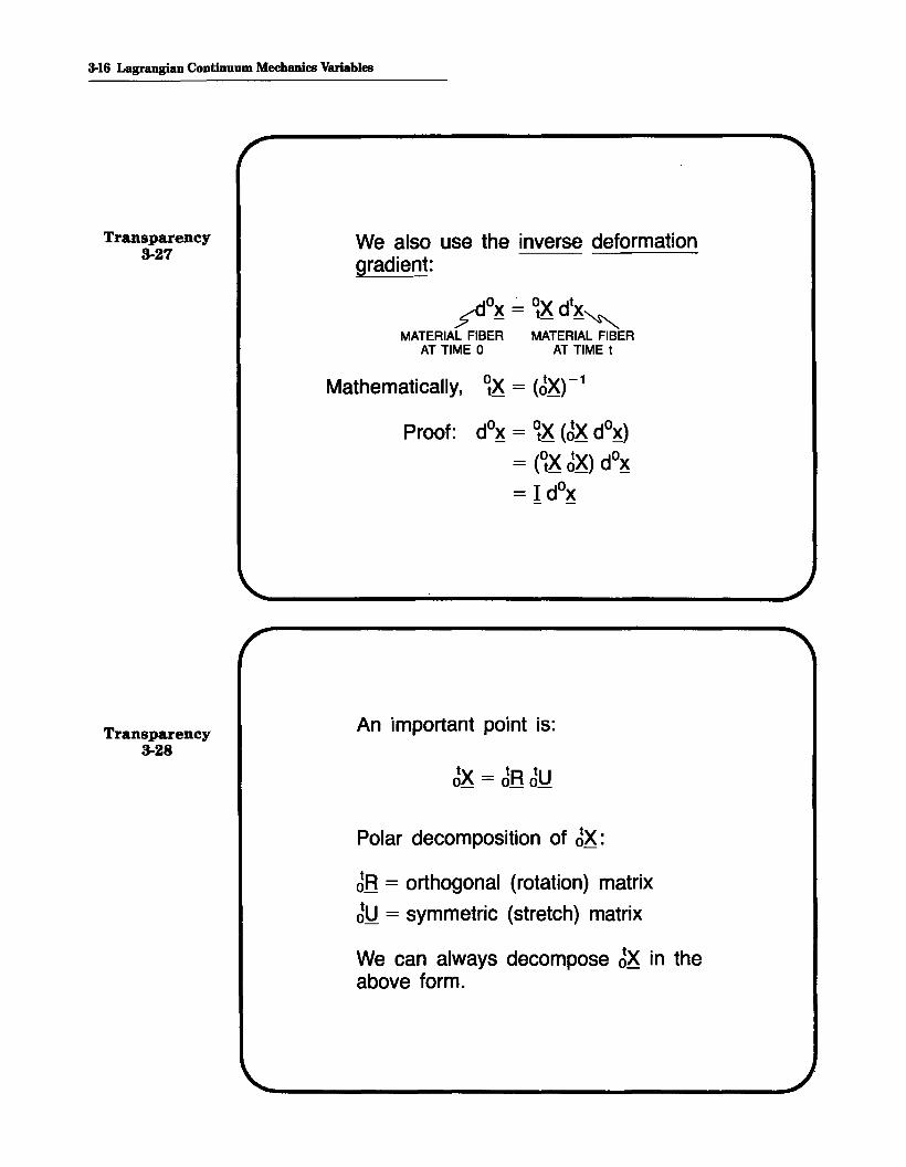
We also use the inverse deformationgradient:

o . 0 t;;{d ~ = tXd~~

MATERIAL FIBER MATERIAL FIBERAT TIME 0 AT TIME t

Mathematically, ~X = (JX)-1

Proof: dO~ = ~ (Jx dO~)

= (~X JX) dO~= I dOx

An important point is:

Polar decomposition of JX:

JR = orthogonal (rotation) matrix

Ju = symmetric (stretch) matrix

We can always decompose JX in theabove form.

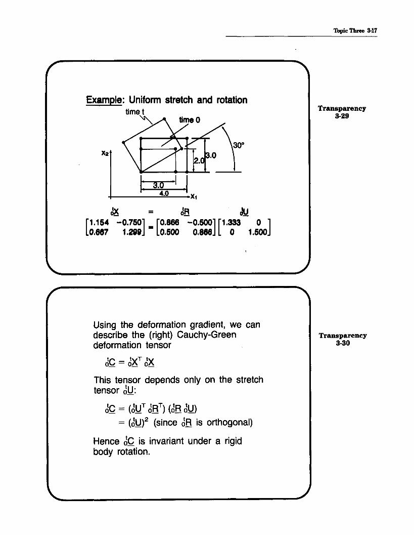
Example: Uniform stretch and rotationtimet~

I: 3.0 I I4.0 X1

~ = dR dU

[1.154 -0.750] .. [0.866 -0.500] [1.333 0]0.887 1.299 0.500 0.888 ° 1.500

Using the deformation gradient, we candescribe the (right) Cauchy-Greendeformation tensor

tc - txT tx0_ - 0_ 0_

This tensor depends only on the stretchtensor riU:

tc = (tuT tAT) (tA tU)0_ 0_ 0_ 0_0_

= (riU)2 (since riA is orthogonal)

Hence ric is invariant under a rigidbody rotation.

Topic Three 3-17

Transparency3-29

Transparency3-30

3·18 Lagrangian Continuum Mechanics Variables

Transparency3-31

Transparency3-32

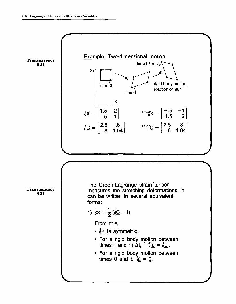
Example: Two-dimensional motion

X2 0 ~ timel+::;U

time'O D rigid body motion,~ rotation of 90°

time t

X1

Jx = [1.5 .~] HatX = [ -.5 -1 ]- .5 0_ 1.5 .2

Jc = [2.5 .8 ] HatC _ [2.5 .8 ]- .8 1.04 0_ - .8 1.04

The Green-Lagrange strain ·tensormeasures the stretching deformations. Itcan be written in several equivalentforms:

1) JE = ~ (ric - I)

From this,

• JE is symmetric.

• For a rigid body motion betweentimes t and t+ ~t, H~E = JE .

• For a rigid body motion betweentimes 0 and t, JE = Q.

• ~~ is symmetric because ~C issymmetric

~~ = ~ (~C -1)

• For a rigid body motion from t tot+~t, we have

t+~tx = R tv0- - 0 0

t+~tc = to j.. t+4t E t0_ 0 ." 0- =o~

• For a rigid body motion

~C = 1 =* ~~ = 0

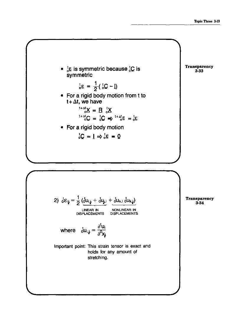
t _ 1 (t t t t )2) aEi} - 2 ,aUi,}:- aU}.~ +, aUk,i ,aUk,} .

UNEAR IN NONUNEAR INDISPLACEMENTS DISPLACEMENTS

Topic Three 3-19

Transparency3-33

Transparency3-34

where

Important point: This strain tensor is exact andholds for any amount ofstretching.

3·20 Lagrangian Continuum Mechanics Variables

Transparency3-35

Transparency3-36

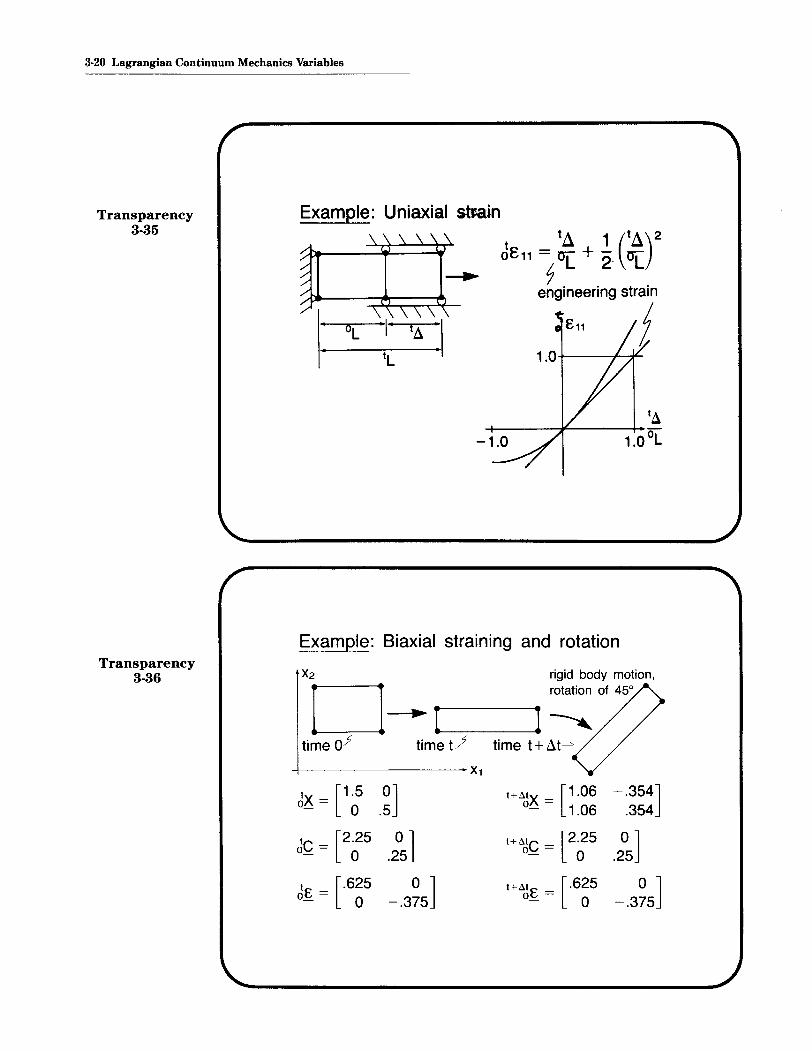
Example: Uniaxial stJlain

tA 1 (tA)2J£11 = 0[ + 2 0[

1engi:~ring 871.o+----+-+-

t~

-~1-.0--~~--1+-.0°L

Example: Biaxial straining and rotation

X2 rigid body motion,

Orotation of 45°

~ I>------l~time 0;7' time t? time t+~t~

+---------X1

IX = [1.5 0]0_ 0.5

ric = [2.25 0 ]- 0 .25

riE = [.625 0 ]- 0 -.375

l+Jllx = [1.060_ 1.06

IHric = [2.25- 0

IHriE = [.625- 0

-.354].354

.~5]

-.3~5]

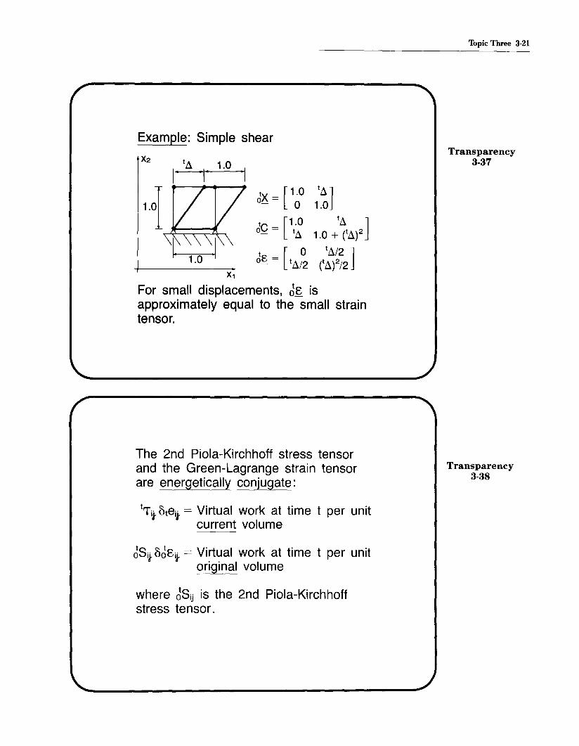
Example: Simple shear

t~ 1.0I' 'I" "

X1

For small displacements, dE isapproximately equal to the small straintensor.

The 2nd Piola-Kirchhoff stress tensorand the Green-Lagrange strain tensorare energetically conjugate:

t'Ti.j- ~hei.j- = Virtual work at time t per unitcurrent volume

Js~ ()JE~ = Virtual work at time t per unitoriginal volume

where dSij is the 2nd Piola-Kirchhoffstress tensor.

Topic Three 3-21

Transparency3-37

Transparency3-38


0tX t'T °tXT- MATRIX NOTATION

o t 0tXi,m 'Tmn tX!-n - INDICIAL NOTATION

Transparency3-39

Transparency3-40

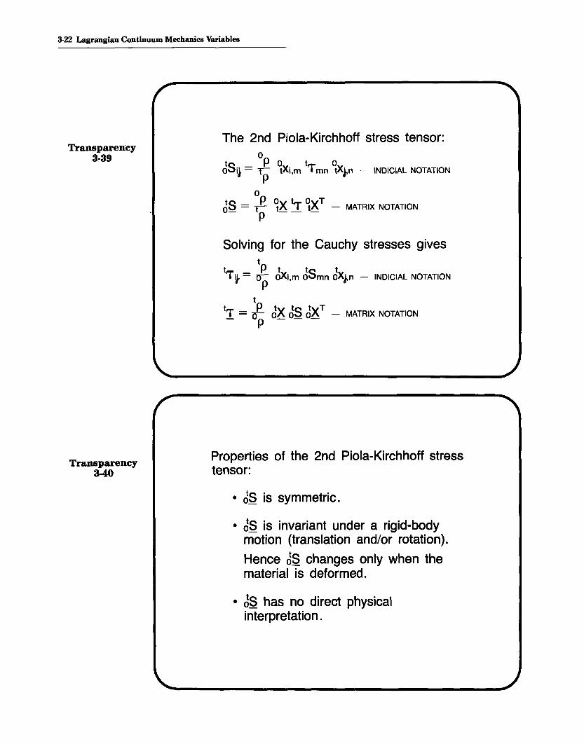
The 2nd Piola-Kirchhoff stress tensor:

t 0pOSi~ =-t

Po

ts = ---.e0_ tp

Solving for the Cauchy stresses givest

t _ P t ts t'Ti~ - op OXi,m 0 mn oXj.n - INDICIAL NOTATION

tt P tx ts txT'T = op 0_ 0_ 0_ - MATRIX NOTATION

Properties of the 2nd Piola-Kirchhoff stresstensor:

• cis is symmetric.

• cis is invariant under a rigid-bodymotion (translation and/or rotation).

Hence cis changes only when thematerial is deformed.

• cis has no direct physicalinterpretation.

Topic Three 3-23

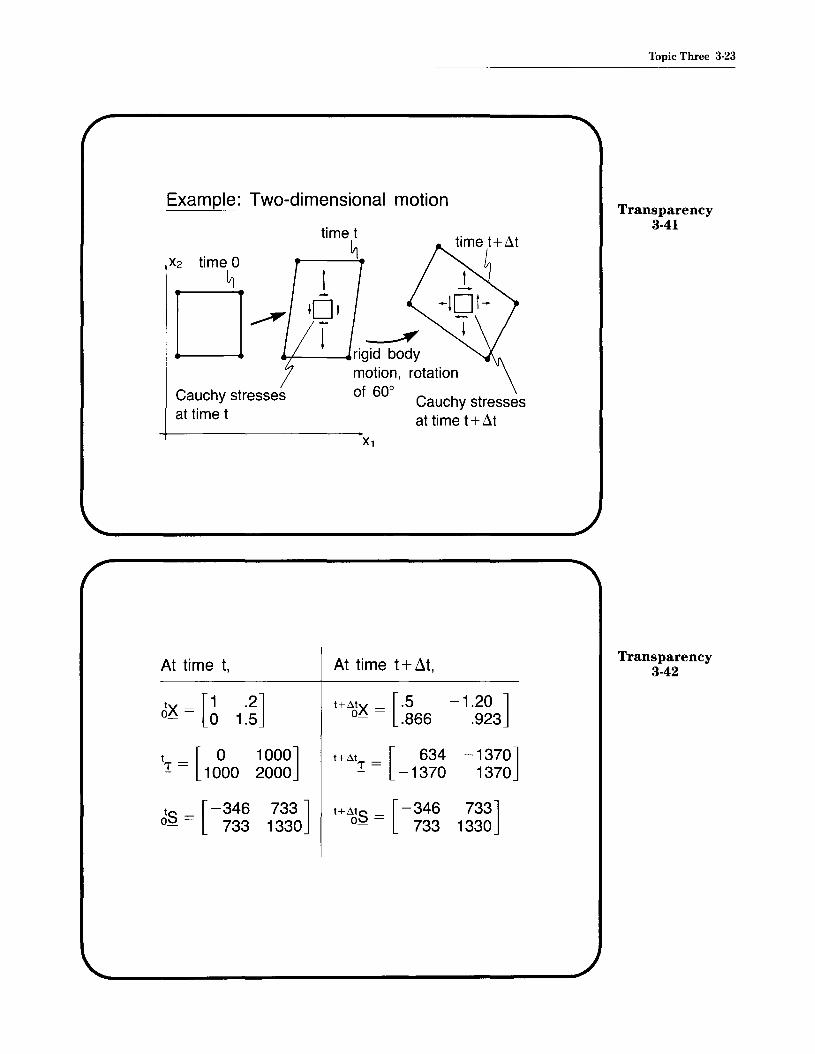
Example: Two-dimensional motionTransparency

3-41

Cauchy stressesat time t

Xi lim\Or~... '__--.. ~..... rigid body

motion, rotationof 60°

Cauchy stressesat time t+ dt

At time t +Llt, TransparencyAt time t, 3-42

tx = [1 .2] t+~tx = [.5 -1.20 ]0_ 0 1.5 0_ .866 .923

t [0 1000] t+ ~t'T = [ 634 -1370]1: = 1000 2000 - -1370 1370

ts _ [ -346 733 ] t+~ts = [ -346 733]0_ - 733 1330 0_ 733 1330

MIT OpenCourseWare http://ocw.mit.edu

Resource: Finite Element Procedures for Solids and Structures Klaus-Jürgen Bathe

The following may not correspond to a particular course on MIT OpenCourseWare, but has been provided by the author as an individual learning resource.

For information about citing these materials or our Terms of Use, visit: http://ocw.mit.edu/terms.

http://ocw.mit.edu

http://ocw.mit.edu/terms

Lagrangian Continuum Mechanics Variables for General Nonlinear

Documents

Transcript of Lagrangian Continuum Mechanics Variables for General Nonlinear