11

Chapter 2. Functional responses in the habitat selection of a

generalist mega-herbivore, the African savannah elephant

Publication Details

Roever, C.L., van Aarde, R.J., Leggett, K., 2012. Functional responses in the habitat selection of a

generalist mega-herbivore, the African savannah elephant. Ecography 35, 972-982. R.J. van Aarde

supervised the study, and R.J. Leggett provided satellite tracking data for 12 elephants in Etosha.

Abstract

Resource selection function (RSF) models are commonly used to quantify species/ habitat

associations and predict species occurrence on the landscape. However, these models are

sensitive to changes in resource availability and can result in a functional response to resource

abundance, where preferences change as a function of availability. For generalist species, which

utilize a wide range of habitats and resources, quantifying habitat selection is particularly

challenging. Spatial and temporal changes in resource abundance can result in changes in

selection preference affecting the robustness of habitat selection models. We examined selection

preference across a wide range of ecological conditions for a generalist mega-herbivore, the

savannah elephant (Loxodonta africana), to quantify general patterns in selection and to illustrate

the importance of functional responses in elephant habitat selection. We found a functional

response in habitat selection across both space and time for tree cover, with tree cover being

unimportant to habitat selection in the mesic, eastern populations during the wet season. A

temporal functional response for water was also evident, with greater variability in selection

12

during the wet season. Selection for low slopes, high tree cover, and far distance from people was

consistent across populations; however, variability in selection coefficients changed as a function

of the abundance of a given resource within the home range. This variability of selection

coefficients could be used to improve confidence estimations for inferences drawn from habitat

selection models. Quantifying functional responses in habitat selection is one way to better

predict how wildlife will respond to an ever-changing environment, and they provide promising

insights into the habitat selection of generalist species.

Introduction

Understanding the complex, dynamic interaction between species occurrence and habitat is

essential to predict and manage responses of species to natural or anthropogenic environmental

changes. Some ecologists therefore rely on resource selection function (RSF) models to quantify

these species/habitat interactions. RSF models compare samples of used and available resource

units to estimate the relative probably of occurrence based on resource characteristics (Boyce et

al. 2002; Manly et al. 2002). This multivariate approach is becoming progressively more flexible

and can incorporate cumulative effects for human development (Houle et al. 2010), intraspecific

competition (McLoughlin et al. 2010), and predation (Hebblewhite et al. 2005). RSF models can

also be used to inform conservation management decisions because they offer spatially explicit

and predictive models of species occurrence (e.g. Aldridge and Boyce 2007; Johnson et al. 2004).

Knowledge of habitat selection is integral for habitat protection and augmentation (Aldridge and

Boyce 2007; Johnson et al. 2004), the reestablishment of species to previously unoccupied habitat

(Merrill et al. 1999), and the identification of dispersal corridors (Chetkiewicz and Boyce 2009) as

well as attractive sinks (Nielsen et al. 2006). Such knowledge may aid in conservation planning

that aims to ensure the viability of a population, the connectivity among sub-populations in a

13

metapopulation, or restore the spatial structuring of populations (e.g. van Aarde and Jackson

2007).

One of the main limitations of RSF models, however, is that the estimate of selection is

contingent upon the sample of availability (Beyer et al. 2010). For example, if use of a resource

remains constant but local availability decreases, then the parameter estimate will change from

avoidance to selection. In a habitat selection framework, this is known as a functional response

(Mysterud and Ims 1998). Functional responses in habitat selection can be an artifact of sampling

intensity (see Beyer et al. 2010), however they can also be driven by behavioural changes is

selection. As a resource becomes more scares on the landscape, an animal needing to meet some

daily requirement, be it nutritional, physiological, or social, must spend a disproportionate

amount of time utilizing that resource. Consequently, selection for a resource changes as a

function of its availability. The presence of a functional response severely limits the application of

an RSF model created for one location to a different area where availability is not equivalent

(Beyer et al. 2010; Boyce et al. 2002; Manly et al. 2002). Under natural conditions resources are

seldom equally available across the distributional range of a species. RSF models therefore are

typically not applied beyond the bounds of a study area unless independent validation data exists

and, when they are, caveats are stipulated. Models that are accurate outside of the study area

are hailed as robust (Boyce et al. 2002; Wiens et al. 2008). Spatially robust models most often

occur for habitat specialists, where species/habitat associations are simple and resilient to

changes in availability (Boyce et al. 2002).

Temporal variation in resource availability can also limit the predictive ability of habitat

selection models (Wiens et al. 2008). Seasonality in resource abundance, even within the same

region, can alter the selection patterns of a species as food preferences change (Boyce et al.

2002). Habitat specialists may be less sensitive to seasonal changes as they are often tied to a

14

single food source or habitat type. For example, northern spotted owls in California are always

closely associated with mature forest (Meyer et al. 1998), and wolverines are closely associated

with high-elevation subalpine habitats (Copeland et al. 2007). Conversely, a generalist species like

grizzly bears have vast shifts in diet (Munro et al. 2006), and consequently habitat selection

preferences change as seasons change (Nielsen et al. 2002).

So what do ecologists do when confronted with a generalist species where habitat

associations are more complex? Boyce et al. (2002) suggest that selection by generalist species be

analyzed across a range of environmental conditions, to quantify how selection changes as a

function of availability. Instead of being viewed as problems to be overcome, functional

responses can instead be used to predict selection in different regions where resources

abundance varies (Boyce et al. 2002; Matthiopoulos et al. 2011). To incorporate a functional

response into an RSF model, a random coefficient in a mixed-effects model can be used (Gillies et

al. 2006; McLoughlin et al. 2010); however, a random coefficient can only be applied to one

habitat covariate within a model. For many generalist species, a functional response is present for

more than one habitat covariate; therefore, separate models are required for each sub-population

(Boyce et al. 2002; Nielsen et al. 2002). The use of separate models also allows one to use the

information theoretic approach to determine whether different habitat covariates are important

in different regions or seasons (Burnham and Anderson 2002).

Despite the call to study multiple populations of generalist species to better understand

patterns in habitat selection, this advice is rarely followed, largely due to the data requirements

for such an analysis. In this paper, we examine habitat selection of a generalist herbivore species,

the African savannah elephant (Loxodonta africana), among seven populations in eight countries

across southern Africa. Elephants are ideally suited for a study on functional responses in habitat

selection because they are widely distributed across southern Africa where they occupy

15

landscapes ranging from the deserts of Namibia to the dense, wet forests of Mozambique. Their

diets also vary seasonally; individuals shift from mainly grazing on tender grasses in the wet

season to mainly browsing on the leaves, twigs, branches, and bark of trees in the dry season

(Codron et al. 2011).

Here, we develop habitat selection models at the scale of the home range that includes

factors elephants are known to respond to: water (de Beer et al. 2006; Harris et al. 2008), slope

(Wall et al. 2006), vegetation structure (Harris et al. 2008; Loarie et al. 2009; Young et al. 2009),

and human presence (Harris et al. 2008; Hoare and du Toit 1999; Jackson et al. 2008). We test for

differences in male and female selection in the wet and dry seasons using the information

theoretic approach to first quantify support for competing models. Then using the full model, we

examine how the selection coefficients changed as a function of availability within an individual’s

home range (Hebblewhite and Merrill 2008; Houle et al. 2010). Our main objective was to

quantify spatial functional responses, examining temporal functional responses only at a course,

two-season scale. Specifically, in the more arid, western portion of the study area, we expect

water and tree cover to be important covariates in habitat use in response to the limited

availability of water (Leggett 2006) and the shortage of trees that provide shade (Kinahan et al.

2007) and offer some forage for elephants (Loarie et al. 2009). In the more mesic, eastern portion

of the study area, we expect elephant’s selection of tree cover to be unimportant for selection

because trees are more plentiful and should, consequently, not limit elephant selection (Illius

2006; Mysterud and Ims 1998). We further expect a functional response to human presence, as

elephants often come into conflict with people (Hoare 1999; Jackson et al. 2008). Thus, elephants

in more remote areas would show greater indifference to human presence.

16

Methods

Study Area

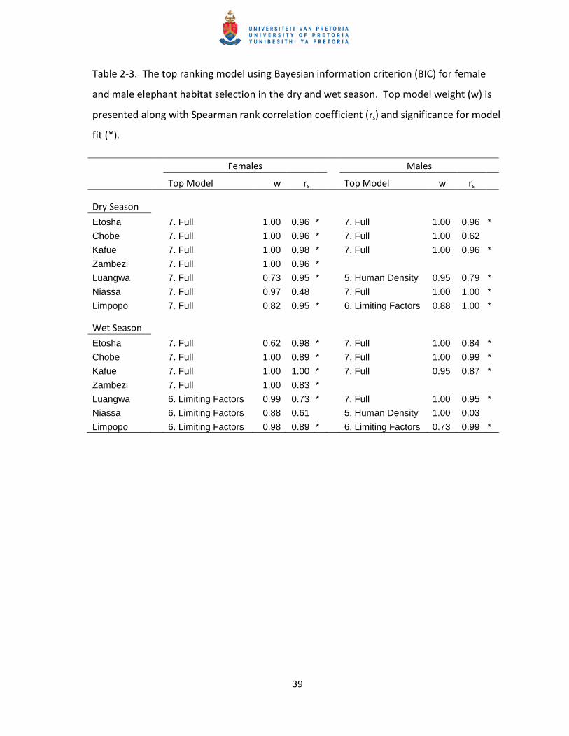
The study area comprised a large portion of the distributional range of elephants in southern

Africa and included portions of Angola, Botswana, Malawi, Mozambique, Namibia, South Africa,

Zambia, and Zimbabwe (Figure 2-1). The region included a desert/grassland mosaic in the west,

dry woodlands in the central region, and mesic forest in the east. Seasonal rainfall patterns drive

vegetation structure (Sankaran et al. 2005). Mesic regions to the east had greater rainfall and

hence greater tree cover compared to western portion of the study area (Table 2-1). Topographic

conditions also varied, with more dramatic changes in elevation near the western and eastern

coasts and relatively flat, unvarying terrain in the central region. Human density was low over

much of the study area, with pockets of increased human densities near major waterways and

roadways.

Elephant Data

Elephants (n=102) were captured and collared with Africa Wildlife Tracking GPS collars (model SM

2000E; Africa Wildlife Tracking, Pretoria, South Africa) between December 2002 and September

2010. Collars were programmed to relocate individuals at varying intervals, ranging from 1 to 24

hours, with most elephants having multiple interval settings during the collaring period.

Telemetry locations were divided into two seasons and combined across years. Core wet season

was defined as December through March inclusive, and core dry season was defined as June

through September (Young et al. 2009). Locations in the transition months of April, May, October,

and November were omitted from the analysis. Only individuals with more than 100 locations per

season were retained for the analysis, resulting in 35,167 locations among 86 individuals for the

dry season and 43,141 locations among 88 individuals for the wet season analysis.

17

Home ranges were generated separately for the core wet and dry season for each

individual using the local convex hull (LoCoH) nonparametric kernel method (Getz et al. 2007).

The adaptive sphere of influence (a-LoCoH) algorithm was used to construct kernels, with a equal

to the furthest distance between any two locations (Getz et al. 2007). LoCoH home ranges, which

ranged in area from 50 to 9,000 km2, fit tightly around telemetry locations often leaving holes,

which we believed were unrealistic. To reduce these holes, home ranges were further buffered by

3 km, the mean distance elephants within our study traveled during a 12 hour period. Home

ranges were created using R software (R Development Core Team 2011), along with the packages

“adehabitat” (Calenge 2006) and “NNCH” (Getz and Wilmers 2004).

The majority of elephants within this study roamed freely and were not confined to parks,

countries, or other intangible human boundaries (van Aarde and Ferreira 2009). However, fences

were present along the borders of Etosha National Park and along international boundaries in

Khaudum Game Reserve and Kruger National Park. For analytical purposes elephants were

grouped by study site, hereby referred to as populations, resulting in seven populations: Etosha,

Chobe, Kafue, Zambezi, Luangwa, Niassa, and Limpopo (ordered from west to northeast, with the

most distant population, Limpopo, last; Figure 2-1). Population names were often based on the

nearest major protected area for convenience.

Habitat Covariates

Habitat covariates were chosen based on their known or suspected influence on elephant space

use. In order to ensure that direct comparisons could be made among models, habitat was

described using covariates that could be applied to all populations, thereby avoiding site-specific

variables such as categorical land cover descriptors. The structure (Harris et al. 2008; Kinahan et

al. 2007) and greenness (Loarie et al. 2009; Young et al. 2009) of vegetation is known to be an

important predictor of elephant space use because it provides both food and shade. Vegetation

18

structure was characterized using the Moderate Resolution Imaging Spectrometer (MODIS)

Vegetation Continuous Fields product (Hansen et al. 2006), from which we estimate the

proportions of tree cover at a resolution of 0.25 km2, defined as woody vegetation greater than 5

m in height (Hansen et al. 2002). An enhanced vegetation index (EVI) was used to quantify

greenness (Pettorelli 2006). For the core wet and dry seasons, EVI layers for the 8 years of this

study were obtained and used to calculate mean EVI within a season at a resolution of 0.64 km2.

Water was located using geospatial data from Tracks4Africa (2010) and man-made

watering point data supplied by conservation authorities. Water body locations were then

validated against Landsat imagery, and missing water bodies were hand-digitized. Separate water

layers were made for each season, with the core wet season including all water categories and the

core dry season including only main rivers, river deltas, lakes, dams, and man-made watering

holes. Distance to water was then calculated for telemetry locations within each season.

Elephants typically avoid humans and human disturbance (Harris et al. 2008; Hoare and

du Toit 1999), particularly during daylight hours when humans are more active (Jackson et al.

2008). We included several covariates that reflect the land-use patterns of people. Human

density was estimated with LandScan (2008) human population data at a resolution of 1 km2.

Hoare and du Toit (1999) found that elephants avoided areas with greater than 15.6 people/ km2;

therefore, we identified areas with greater than 16 people/ km2 (rounding up) and calculated the

distance from each elephant location to these pixels. Road data were obtained from Tracks4Africa

(2010). Studies of other large mammals have shown an avoidance of high-traffic volume roads

but neutral or positive selection for low-traffic volume roads which potentially facilitate

movement (Chruszcz et al. 2003; Dickson et al. 2005); therefore, roads were categorized based on

size. We determined distances of locations to main roads (freeway, national, or main roads) and

secondary roads (all other road categories).

19

Finally, elephants avoid steep slopes due to their large body size (Wall et al. 2006), so we

included slope derived from a 90 x 90 m resolution digital elevation model (Jarvis et al. 2006) in

our analyses. All geospatial analysis was completed using the Spatial Analyst extension of ArcGIS

9.3.1 (ESRI 2009) and Geospatial Modelling Environment (Beyer 2011).

Habitat Selection Models

Habitat selection was modelled separately for the seven elephant populations and for males and

females, with one collared female actually representing a breeding herd with several adult

females and their offspring. Elephant locations (1) were compared to randomly generated

locations (0) using a mixed effect logistic regression model for location i and individual j, taking the

form:

w(xij) = exp(β + β1x1ij+ …+ βnxnij + γj), (1)

where w(xij) is the resource selection function, βn is the coefficient for the n-th predictor variable

xn , and γ is the random intercept for animal j (Gillies et al. 2006; Manly et al. 2002). The random

intercept was used to control for the lack of independence of points within individuals and

differences in sample size among individuals (Gillies et al. 2006). We implemented a design III

approach (Manly et al. 2002; Thomas and Taylor 1990), whereby random locations were

generated within the home range of each elephant at a density of 3 points/km2. At this density,

contamination (i.e. use and available locations occurring within the same raster pixel) was less

than 15% for the habitat covariate mapped at the coarsest resolution (800 x 800 m), and was

therefore negligible (Johnson et al. 2006).

We used model selection (Burnham and Anderson 2002) to determine which habitat

covariates had the greatest influence on resource selection for each of the seven populations.

Seven a priori candidate models were ranked using Bayesian Information Criterion (BIC; Table 2-

20

2). BIC was used as it favours more parsimonious models compared to Akaike’s Information

Criterion (AIC), which favours complex models when sample sizes are large (Burnham and

Anderson 2002; Grueber et al. 2011). Variables that were highly correlated (Pearson’s r > 0.6)

were not included in the same model. Correlations occurred between tree cover and mean EVI

(Pearson’s r = 0.68). Because tree cover is an indicator of both food resources and

thermoregulatory needs (i.e. shade cover; Kinahan et al. 2007), tree cover was used in subsequent

models. All continuous variables were tested for the potential presence of a nonlinear

relationship with the inclusion of a quadratic term in a univariate analysis and by examining

histograms. Model fit of the top-ranked model for each population was evaluated using k-fold

cross validation (k = 5) and the Spearman rank correlation coefficient (Boyce et al. 2002). Analyses

were conducted in R software (R Development Core Team 2011) using the lme4 package (Bates

and Maechler 2010).

To test the presence of functional responses, we used a two-step approach (Hebblewhite

and Merrill 2008; Houle et al. 2010). First we model habitat selection for each individual, so that

all covariates could vary in slope and intercept, using the full model (model 7, Table 2-2). We then

assessed how the selection coefficient of a given covariate changed as a function of the mean

value of that covariate within the individual’s home range (log transformed). Significance was

evaluated using a linear regression. Where models displayed heterogeneity of variance,

generalized least squares were used instead of a simple linear regression (Zuur et al. 2010). This

procedure could only be applied to covariates with linear selection coefficients (i.e. slope,

proportion tree, distance to people, and distance to main roads).

21

Results

Dry Season RSF Models

The top-ranked model was the full model (model 7) for all female and most male (4 of 6)

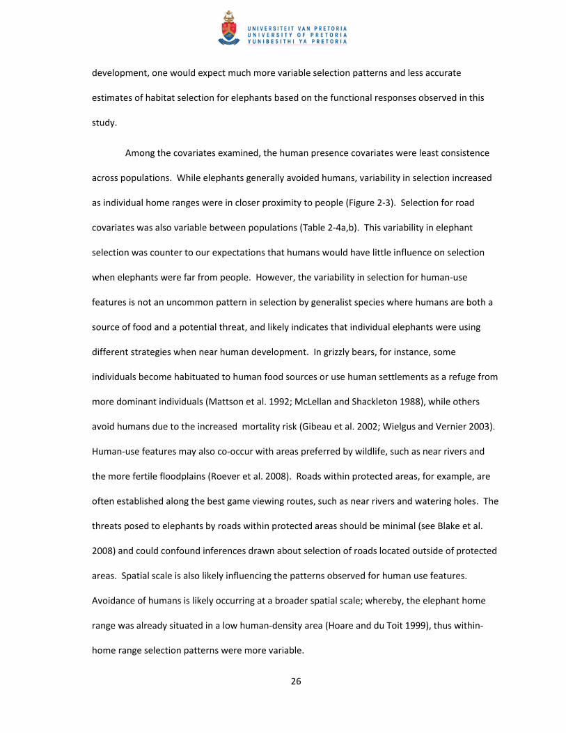
populations during the dry season (Table 2-3). The top models provided good fit to the data using

k-fold cross validation expect for Niassa females (Spearman rank rs = 0.48, and p > 0.05) and

Chobe males (rs = 0.62, and p > 0.05; Table 2-3). The inclusion of all variables in most top-ranked

models was counter to our expectations that selection for some covariates would be less

important as availability changed. This indicated that all variables examined in this study were

important to elephant habitat selection irrespective of availability during the dry season. The

strength and direction of covariates was consistent across most populations in the top-ranked

models. Elephants from most populations selected areas of low slope (female (f) = 5 of 7, male

(m) = 4 of 6), high tree cover (f = 7 of 7, m = 3 of 6), far distances from people (f = 4 of 7, m = 4 of

6), and close proximity to main road (f = 3 of 7, m = 5 of 6; Table 2-4). Populations varied in the

maximum distance elephants traveled from water, ranging from 6 km in the Zambezi to 79 km in

the Chobe population. Despite this, elephants in most populations (f = 4 of 7, m = 5 of 6) selected

areas near and far from water at greater frequencies than random (Table 2-4; Figure 2-2). This U-

shaped pattern is what I expected as animals select areas near water for drinking and temperature

regulation and far from water in search of forage. Only Niassa females selected areas of

intermediate distances from water during the dry season (i.e. the selection coefficient had a

hump-shaped curve). Selection for secondary roads was less consistent across populations.

Males and females in Niassa and Limpopo along with Etosha females and Chobe males selected

areas of intermediate distance from secondary roads; whereas, the elephants from the remaining

populations selected areas near to secondary roads or areas both near and far from these roads.

22

Wet Season RSF Models

In the wet season, Etosha, Chobe, Kafue, and Zambezi populations continued to have the full

model (model 7) as the top-ranked model for both sexes (Table 2-3). However, among the more

easterly populations, Luangwa, Niassa, and Limpopo, the top-ranked model was the limiting

factors model (model 6) for those females and for Limpopo males. Of these eastern populations,

only Luangwa males had a top-ranked model that included tree cover, indicating that during the

wet season tree cover was not an important predictor of elephant habitat selection in these

populations. This was concurrent with our expectations that tree cover would be less influential

for elephants in more mesic environments. The top models provided good fit for most

populations during the wet season; however, model fit was poor for Niassa females and males (rs

= 0.61 and 0.03, respectively, and p > 0.05; Table 2-3). Selection for water during the wet season

was more variable across populations than it was in the dry season. Luangwa and Limpopo

females selected areas both near and far from water, Zambezi and Chobe females selected

intermediate distance from water, Kafue and Niassa females selected areas close to water, and

Etosha females selected areas far from water. Half of the male populations (3 of 6) selected areas

both near and far from water, while the remaining three were variable in selection (Figure 2-2).

This variability in selection indicated a functional response to water seasonally. Selection for low

slopes (f = 5 of 7, m = 3 of 6), high tree cover (f = 4 of 7, m = 3 of 6), and far from people (f = 4 of 7,

m = 3 of 6) was similar to the dry season. However, selection for main roads was counter to dry

season selection, with nearly equal numbers avoiding (f = 3 of 7, m = 3 of 6) and selecting (f = 4 of

7, m = 3 of 6) main roads. In the wet season, selection for secondary roads continued to be as

variable as it was in the dry season.

23

Functional Responses

When comparing the selection coefficient for a given covariate to the mean value of that covariate

within an individual’s home range, we found a significant functional response for proximity to

humans during the dry season (R2 adjusted=0.04, P = 0.03; Figure 2-3). As the mean distance from

humans increased (i.e. as there were fewer people within the home range) selection for proximity

to people decreased. We expected selection for proximity to human to be less significant when

elephants were far from human development; however, we did not find this pattern. Instead, we

found a general pattern of avoidance when they were far from people and high heterogeneity in

the selection coefficient when elephants were close to people.

While the functional responses tested were not significant within a linear regression

model for all other covariates examined, the variability of selection coefficients at varying levels of

resource abundance indicated similar patterns as observed with the proximity to humans

covariate. Because of heterogeneity of variance in the slope and tree cover models, generalized

least squares techniques were used. While most elephants selected areas of low slope, when the

home range of an individual was located in a relatively flat area, the selection coefficient was

more variable (Figure 3). A similar pattern occurred with tree cover. When the proportion of tree

cover within an individual’s home range was low, the variability in the selection coefficient

increased with some individuals having relatively strong selection for trees. Functional responses

for distance to main road were not significant during either season and displayed no variance in

heterogeneity.

Discussion

Although elephants are generalist mega-herbivores with wide ecological tolerances, we found

consistency in their habitat selection patterns, lending insight into the biology of the species.

24

Elephants in most populations and both seasons had the full model (model 7) as the top-ranked

BIC model. This is not unexpected given that for inclusion in BIC models, we considered covariates

which relate to some biological process or limiting factor for elephants (e.g. food, water, terrain,

and human presence). We did, however, find that in the wetter, eastern populations (Luangwa,

Niassa, and Limpopo) tree cover was not an important predictor of elephant use in the wet

season, as expected. The decline in the importance of the vegetation covariate suggested a

functional response for vegetation, where its importance declines both temporally (within these

populations as increased rainfall makes food more readily available) and spatially (across

populations as vegetative cover increases). This functional response was not supported when we

examined the abundance of tree cover within each individual’s home range. However, when we

further excluded non-significant selection coefficients from the analysis to reflect their lack of

importance in those models, the function response was significant in the dry season (P = 0.02).

Our results also revealed evidence of a temporal functional response for water. Water is a

limiting factor for elephants, as demonstrated by their close association with watering holes in the

dry season (de Beer et al. 2006; Harris et al. 2008; Shannon et al. 2009; Young et al. 2009) and

their population increases when supplemental water is provided (Owen-Smith et al. 2006). In the

dry season, elephants in most populations (f = 4 of 7, m = 5 of 6) selected areas near and far

water; whereas, in the wet season, selection for water was highly variable, with individuals

selecting areas near, far, and at intermediate distance from water (Figure 2-2). The change in

selection for water as a function of season suggests a functional response, as higher rainfall during

the wet season results in greater abundance and wider distribution of water throughout the study

area. However, we did not find a spatial functional response for water as expected. The more

mesic, eastern populations had similar selection patterns for water in the dry season, indicating

that water was a limiting factor, even in these wetter regions.

25

Selection for low slopes, high tree cover, and far distance from people was consistent

across populations and seasons and was similar to previous studies of elephant selection patterns

(see Harris et al. 2008; Hoare and du Toit 1999; Kinahan et al. 2007; Loarie et al. 2009; Wall et al.

2006). The real ecological insight gained from studying elephant selection across a large spatial

scale, however, comes from the heterogeneity of variance displayed in the functional responses.

Previous research into function responses of habitat selection has not reported such

heterogeneity in variance. This could be an artifact of low sample size, as most studies have few

individuals along the continuum of available abundance (see Hebblewhite and Merrill 2008; Houle

et al. 2010). However, heterogeneity of variance in habitat selection should be expected for some

habitat covariates. Slope, for example, does not limit elephant movement when the home range

is situated in a relatively flat area. As a result, we found high variability in the selection

coefficients in these locations. When elephant home ranges occur in regions of high topographic

variation, slope became a limiting factor and, consequently, the selection coefficients were

consistently negative (i.e. elephants selected flat areas; Figure 2-3).

One of the main criticisms of RSF models is that they are limited in their ability to make

predictions in different areas or at different times (Garshelis 2000; Manly et al. 2002). Some

authors contend that using information gained about functional responses in selection could help

remedy this problem (Boyce et al. 2002; Matthiopoulos et al. 2011; McLoughlin et al. 2010). For

elephants, selection at the scale measured in this study was relatively consistent and the

measured functional responses were not significant; consequently, we do not believe that the

function responses discovered here could be used towards those ends. However, researchers

could use information about heterogeneity of variance to better estimate the confidence around

habitat selection models applied to new regions, especially when no data on animal use is

available. If, for example, an area was relatively flat in slope or was in close proximity to human

26

development, one would expect much more variable selection patterns and less accurate

estimates of habitat selection for elephants based on the functional responses observed in this

study.

Among the covariates examined, the human presence covariates were least consistence

across populations. While elephants generally avoided humans, variability in selection increased

as individual home ranges were in closer proximity to people (Figure 2-3). Selection for road

covariates was also variable between populations (Table 2-4a,b). This variability in elephant

selection was counter to our expectations that humans would have little influence on selection

when elephants were far from people. However, the variability in selection for human-use

features is not an uncommon pattern in selection by generalist species where humans are both a

source of food and a potential threat, and likely indicates that individual elephants were using

different strategies when near human development. In grizzly bears, for instance, some

individuals become habituated to human food sources or use human settlements as a refuge from

more dominant individuals (Mattson et al. 1992; McLellan and Shackleton 1988), while others

avoid humans due to the increased mortality risk (Gibeau et al. 2002; Wielgus and Vernier 2003).

Human-use features may also co-occur with areas preferred by wildlife, such as near rivers and

the more fertile floodplains (Roever et al. 2008). Roads within protected areas, for example, are

often established along the best game viewing routes, such as near rivers and watering holes. The

threats posed to elephants by roads within protected areas should be minimal (see Blake et al.

2008) and could confound inferences drawn about selection of roads located outside of protected

areas. Spatial scale is also likely influencing the patterns observed for human use features.

Avoidance of humans is likely occurring at a broader spatial scale; whereby, the elephant home

range was already situated in a low human-density area (Hoare and du Toit 1999), thus within-

home range selection patterns were more variable.

27

Other variables also display variability, even within the same population. Selection for

tree cover, for example, was positive for females in Etosha in both seasons, yet negative for males

in both seasons. This variability is selection patterns is likely an artifact of a collaring bias for the

Etosha cluster. In the bounds of Etosha NP only females were collared (n = 9 females), and

outside of the park boundaries, mostly males (8 of 9) were collared. This shows the sensitivity of

RSF models to local resources availability, and that even within close, yet non-overlapping,

proximity changes in availability can produce opposing habitat selection patterns. It also further

underscores the need to quantify how selection changes and a function of resource availability.

This study represents an amalgamation of habitat selection theory for elephants across

southern Africa; however, a study area of this magnitude, particularly in the developing world,

creates unique challenges. To make comparisons across regions, the habitat covariates chosen

had to be consistent across the study area. Unfortunately, GIS data quality often varies from one

country to the next, so while detailed geospatial data were available for South Africa, Namibia,

and Mozambique, information was often lacking for Malawi, Zambia, and Zimbabwe.

Consequently, we used global datasets which, while excellent in quality, use larger spatial

resolution (the smallest being 90 x 90 m for slope but increasing to 500 x 500 m for tree cover).

This larger resolution could help explain the poor model fit for Niassa females and Chobe males in

the dry season and Niassa females and males in the wet season. Prediction of elephant habitat

selection could be improved if fine scale information on vegetation characteristics and the

presence of standing water across the seasons were available. As some of the world’s most

diverse and valuable wildlife resources are in the developing world, efforts should be made to

increase the quality of geospatial data in these regions for the betterment of wildlife

management.

28

Studying a generalist species over a wide spatial scale can lend insight into the biology of

that species (Boyce et al. 2002), which could be particularly important in predicting changes in

animal space-use in this ever-changing world. Our analysis confirms expectations that a generalist

mega-herbivore showed a functional response, particularly when the relevant resource was

uncommon or limiting (Illius 2006; Mysterud and Ims 1998). We also found that selection by this

generalist species is more variable when at different levels of resource abundance, which can be

used to better estimate confidence around model predictions. In southern Africa, elephant

management strategies are moving towards reinstating a more natural, self-sustaining spatial

dynamic through the development of transfrontier conservation areas (see Hanks 2001; van Aarde

and Jackson 2007; Western 2003). Current initiatives strive to remove fences around parks,

reduce artificial water sources, and promote cooperation between countries, allowing wildlife

access to greater and more natural roaming areas. However, information on how elephants will

respond to these changes is lacking because experimentation on many large mammal species,

particularly those of management concern, is not feasible. Consequently, researchers must work

within the context of present-day landscapes, and these conservation initiatives can benefit from

relying on our illustrated functional responses to better predict elephant selection within these

changing landscapes.

Acknowledgements

Support for this study was provide by Billiton, Conservation Foundation Zambia, Conservation

International’s southern Africa’s Wildlife Programme, the Conservation Lower Zambezi, Duke

University, the International Fund for Animal Welfare, the Mozal Community Development Trust,

the National Research Foundation, the National Postcode Lottery of the Netherlands, Peace Parks

Foundation, the US Fish and Wildlife Services, the University of Pretoria, the World Wildlife Fund

(SARPO; Mozambique; SA), the Walt Disney Grant Foundation, and the Wildlifewins Lottery.

29

Logistical support was provided by Bateleurs, South African National Parks, Tracks4Africa, and

Wings for Wildlife. This research was sanctioned and supported by the Botswana Department of

Wildlife & National Parks, Direcção Nacional de Areas de Conservação, the Namibian Ministry of

Tourism & Environment, the Malawian Wildlife Department, Ezemvelo KZN Wildlife of South

Africa, and the Zambian Wildlife Authority.

30

References

Aldridge, C.L., Boyce, M.S., 2007. Linking occurrence and fitness to persistence: Habitat-based

approach for endangered Greater Sage-Grouse. Ecological Applications 17, 508-526.

Bates, D., Maechler, M., 2010. Linear mixed-effects models using S4 classes. R package version

0.999375-37.

Beyer, H.L., 2011. Geospatial Modelling Environment. Spatial Ecology, LLC.

http://www.spatialecology.com/gme/.

Beyer, H.L., Haydon, D.T., Morales, J.M., Frair, J.L., Hebblewhite, M., Mitchell, M., Matthiopoulos,

J., 2010. The interpretation of habitat preference metrics under use-availability designs.

Philosophical Transactions of the Royal Society B-Biological Sciences 365, 2245-2254.

Blake, S., Deem, S.L., Strindberg, S., Maisels, F., Momont, L., Isia, I.B., Douglas-Hamilton, I., Karesh,

W.B., Kock, M.D., 2008. Roadless wilderness area determines forest elephant movements

in the Congo Basin. PLoS ONE 3, e3546.

Boyce, M.S., Vernier, P.R., Nielsen, S.E., Schmiegelow, F.K.A., 2002. Evaluating resource selection

functions. Ecological Modelling 157, 281-300.

Burnham, K.P., Anderson, D.R., 2002. Model Selection and Multimodel Inference: A practical

information-theoretic approach, 2nd edn. Springer-Verlag, New York.

Calenge, C., 2006. The package "adehabitat" for the R software: A tool for the analysis of space

and habitat use by animals. Ecological Modelling 197, 516-519.

Chetkiewicz, C.L.B., Boyce, M.S., 2009. Use of resource selection functions to identify conservation

corridors. Journal of Applied Ecology 46, 1036-1047.

Chruszcz, B., Clevenger, A.P., Gunson, K.E., Gibeau, M.L., 2003. Relationships among grizzly bears,

highways, and habitat in the Banff-Bow Valley, Alberta, Canada. Canadian Journal of

Zoology-Revue Canadienne De Zoologie 81, 1378-1391.

31

Codron, J., Codron, D., Lee-Thorp, J.A., Sponheimer, M., Kirkman, K., Duffy, K.J., Sealy, J., 2011.

Landscape-scale feeding patterns of African elephant inferred from carbon isotope

analysis of feces. Oecologia 165, 89-99.

Copeland, J.P., Peek, J.M., Groves, C.R., Melquist, N.E., McKelvey, K.S., McDaniel, G.W., Long, C.D.,

Harris, C.E., 2007. Seasonal habitat associations of the wolverine in central Idaho. Journal

of Wildlife Management 71, 2201-2212.

de Beer, Y., Kilian, W., Versfeld, W., van Aarde, R.J., 2006. Elephants and low rainfall alter woody

vegetation in Etosha National Park, Namibia. Journal of Arid Environments 64, 412-421.

Dickson, B.G., Jenness, J.S., Beier, P., 2005. Influence of vegetation, topography, and roads on

cougar movement in southern California. Journal of Wildlife Management 69, 264-276.

ESRI, 2009. ArcGIS version 9.3.1. Environmental Systems Research Institute (ESRI), Redlands.

Garshelis, D.L., 2000. Delusions in habitat evaluation: measureing use, selection, and importance,

In Research Techniques in Animal Ecology: Controversies and Consequences. eds L.

Boitani, T.K. Fuller, pp. 111-164. Columbia University Press, New York.

Getz, W.M., Fortmann-Roe, S., Cross, P.C., Lyons, A.J., Ryan, S.J., Wilmers, C.C., 2007. LoCoH:

Nonparameteric kernel methods for constructing home ranges and utilization

distributions. PLoS ONE 2, e207.

Getz, W.M., Wilmers, C.C., 2004. A local nearest-neighbor convex-hull construction of home

ranges and utilization distributions. Ecography 27, 489-505.

Gibeau, M.L., Clevenger, A.P., Herrero, S., Wierzchowski, J., 2002. Grizzly bear response to human

development and activities in the Bow River Watershed, Alberta, Canada. Biological

Conservation 103, 227-236.

32

Gillies, C.S., Hebblewhite, M., Nielsen, S.E., Krawchuk, M.A., Aldridge, C.L., Frair, J.L., Saher, D.J.,

Stevens, C.E., Jerde, C.L., 2006. Application of random effects to the study of resource

selection by animals. Journal of Animal Ecology 75, 887-898.

Grueber, C.E., Nakagawa, S., Laws, R.J., Jamieson, I.G., 2011. Multimodel inference in ecology and

evolution: Challenges and solutions. Journal of Evolutionary Biology 24, 699-711.

Hanks, J., 2001. Conservation strategies for Africa's large mammals. Reproductive Fertility and

Development 13, 459-468.

Hansen, M., DeFries, R.S., Townshend, J.R., Carroll, M., Dimiceli, C., Sohlberg, R., 2006. Vegetation

Continuous Fields MOD44B, 2001 Percent Tree Cover, Collection 4. University of

Maryland, College Park, Maryland, 2001.

Hansen, M.C., DeFries, R.S., Townshend, J.R.G., Sohlberg, R., Dimiceli, C., Carroll, M., 2002.

Towards an operational MODIS continuous field of percent tree cover algorithm:

examples using AVHRR and MODIS data. Remote Sensing of Environment 83, 303-319.

Harris, G.M., Russell, G.J., van Aarde, R.I., Pimm, S.L., 2008. Rules of habitat use by elephants

Loxodonta africana in southern Africa: insights for regional management. Oryx 42, 66-75.

Hebblewhite, M., Merrill, E., 2008. Modelling wildlife-human relationships for social species with

mixed-effects resource selection models. Journal of Applied Ecology 45, 834-844.

Hebblewhite, M., Merrill, E.H., McDonald, T.L., 2005. Spatial decomposition of predation risk using

resource selection functions: an example in a wolf-elk predator-prey system. Oikos 111,

101-111.

Hoare, R.E., 1999. Determinants of human-elephant conflict in a land-use mosaic. Journal of

Applied Ecology 36, 689-700.

Hoare, R.E., du Toit, J.T., 1999. Coexistence between people and elephants in African savannas.

Conservation Biology 13, 633-639.

33

Houle, M., Fortin, D., Dussault, C., Courtois, R., Ouellet, J.P., 2010. Cumulative effects of forestry

on habitat use by gray wolf (Canis lupus) in the boreal forest. Landscape Ecology 25, 419-

433.

Illius, A.W., 2006. Linking functional responses and foraging behavior to population dynamics, In

Large Herbivore Ecology, Ecosystem Dynamics, and Conservation. eds K. Danell, P.

Duncan, R. Bergstrom, J. Pastor, pp. 71-96. Cambridge University Press, Cambridge.

Jackson, T.R., Mosojane, S., Ferreira, S.M., van Aarde, R.J., 2008. Solutions for elephant Loxodonta

africana crop raiding in northern Botswana: moving away from symptomatic approaches.

Oryx 42, 83-91.

Jarvis, A., Reuter, H.I., Nelson, A., Guevara, E., 2006. Hole-filled seamless SRTM data V3.

International Centre for Tropical Agriculture (CIAT). http://srtm.csi.cgiar.org.

Johnson, C.J., Nielsen, S.E., Merrill, E.H., McDonald, T.L., Boyce, M.S., 2006. Resource selection

functions based on use-availability data: Theoretical motivation and evaluation methods.

Journal of Wildlife Management 70, 347-357.

Johnson, C.J., Seip, D.R., Boyce, M.S., 2004. A quantitative approach to conservation planning:

using resource selection functions to map the distribution of mountain caribou at multiple

spatial scales. Journal of Applied Ecology 41, 238-251.

Kinahan, A.A., Pimm, S.L., van Aarde, R.J., 2007. Ambient temperature as a determinant of

landscape use in the savanna elephant, Loxodonta africana. Journal of Thermal Biology 32,

47-58.

LandScan, 2008. High Resolution global Population Data Set. Copyrighted by UT-Battelle, LLC,

operator of Oak Ridge National Laboratory under Contract No. DE-AC05-00OR22725 with

the United States Department of Energy.

34

Leggett, K., 2006. Effect of artificial water points on the movement and behaviour of desert-

dwelling elephants of north-western Namibia. Pachyderm 40, 40-51.

Loarie, S.R., van Aarde, R.J., Pimm, S.L., 2009. Elephant seasonal vegetation preferences across dry

and wet savannas. Biological Conservation 142, 3099-3107.

Manly, B.F.J., McDonald, L.L., Thomas, D.L., McDonald, T.L., Erickson, W.P., 2002. Resource

Selection by Animals: Statistical Design and Analysis for Field Studies, 2 edn. Kluwer

Academic Publishers, Dordrecht.

Matthiopoulos, J., Hebblewhite, M., Aarts, G., Fieberg, J., 2011. Generalized functional responses

for species distributions. Ecology 92, 583-589.

Mattson, D.J., Blanchard, B.M., Knight, R.R., 1992. Yellowstone grizzly bear mortality, human

habituation, and whitebark-pine seed crops. Journal of Wildlife Management 56, 432-442.

McLellan, B.N., Shackleton, D.M., 1988. Grizzly bears and resource-extraction industries - Effects

of roads on behavior, habitat use and demography. Journal of Applied Ecology 25, 451-

460.

McLoughlin, P.D., Morris, D.W., Fortin, D., Vander Wal, E., Contasti, A.L., 2010. Considering

ecological dynamics in resource selection functions. Journal of Animal Ecology 79, 4-12.

Merrill, T., Mattson, D.J., Wright, R.G., Quigley, H.B., 1999. Defining landscapes suitable for

restoration of grizzly bears Ursus arctos in Idaho. Biological Conservation 87, 231-248.

Meyer, J.S., Irwin, L.L., Boyce, M.S., 1998. Influence of habitat abundance and fragmentation on

northern spotted owls in western Oregon. Wildlife Monographs 139, 5-51.

Munro, R.H.M., Nielsen, S.E., Price, M.H., Stenhouse, G.B., Boyce, M.S., 2006. Seasonal and diel

patterns of grizzly bear diet and activity in west-central Alberta. Journal of Mammalogy

87, 1112-1121.

35

Mysterud, A., Ims, R.A., 1998. Functional responses in habitat use: Availability influences relative

use in trade-off situations. Ecology 79, 1435-1441.

Nielsen, S.E., Boyce, M.S., Stenhouse, G.B., Munro, R.H.M., 2002. Modeling grizzly bear habitats in

the yellowhead ecosystem of Alberta: Taking autocorrelation seriously. Ursus 13, 45-56.

Nielsen, S.E., Stenhouse, G.B., Boyce, M.S., 2006. A habitat-based framework for grizzly bear

conservation in Alberta. Biological Conservation 130, 217-229.

Owen-Smith, N., Kerley, G.I.H., Page, B., Slotow, R., van Aarde, R.J., 2006. A scientific perspective

on the management of elephants in the Kruger National Park and elsewhere. South

African Journal of Science 102, 389-394.

Pettorelli, N., 2006. Using the satellite-derived NDVI to assess ecological responses to

environmental change (vol 20, pg 503, 2005). Trends in Ecology & Evolution 21, 11-11.

R Development Core Team, 2011. R: A language and environment for statistical computing. R

Foundation for Statistical Computing, Vienna, Austria. ISBN 3-900051-07-0.

http://www.R-project.org.

Roever, C.L., Boyce, M.S., Stenhouse, G.B., 2008. Grizzly bears and forestry II: Grizzly bear habitat

selection and conflicts with road placement. Forest Ecology and Management 256, 1262-

1269.

Sankaran, M., Hanan, N.P., Scholes, R.J., Ratnam, J., Augustine, D.J., Cade, B.S., Gignoux, J.,

Higgins, S.I., Le Roux, X., Ludwig, F., Ardo, J., Banyikwa, F., Bronn, A., Bucini, G., Caylor,

K.K., Coughenour, M.B., Diouf, A., Ekaya, W., Feral, C.J., February, E.C., Frost, P.G.H.,

Hiernaux, P., Hrabar, H., Metzger, K.L., Prins, H.H.T., Ringrose, S., Sea, W., Tews, J.,

Worden, J., Zambatis, N., 2005. Determinants of woody cover in African savannas. Nature

438, 846-849.

36

Shannon, G., Matthews, W.S., Page, B.R., Parker, G.E., Smith, R.J., 2009. The affects of artificial

water availability on large herbivore ranging patterns in savanna habitats: a new approach

based on modelling elephant path distributions. Diversity and Distributions 15, 776-783.

Thomas, D.L., Taylor, E., 1990. Study designs and tests for comparing resource use and

availability. Journal of Wildlife Management 54, 322-330.

Tracks4Africa, 2010. Tracks4Africa Enterprises (Pty) Ltd. Unit 8 Innovation Center, Electron Street,

Techno Park, Stellenbosch, 7599, Western Cape, South Africa. http://tracks4africa.co.za/.

van Aarde, R.J., Ferreira, S.M., 2009. Elephant populations and CITES trade resolutions.

Environmental Conservation 36, 8-10.

van Aarde, R.J., Jackson, T.P., 2007. Megaparks for metapopulations: Addressing the causes of

locally high elephant numbers in southern Africa. Biological Conservation 134, 289-297.

Wall, J., Douglas-Hamilton, I., Vollrath, F., 2006. Elephants avoid costly mountaineering. Current

Biology 16, 527-529.

Western, D., 2003. Conservation science in Africa and the role of international collaboration.

Conservation Biology 17, 11-19.

Wielgus, R.B., Vernier, P.R., 2003. Grizzly bear selection of managed and unmanaged forests in the

Selkirk Mountains. Canadian Journal of Forest Research-Revue Canadienne De Recherche

Forestiere 33, 822-829.

Wiens, T.S., Dale, B.C., Boyce, M.S., Kershaw, G.P., 2008. Three way k-fold cross-validation of

resource selection functions. Ecological Modelling 212, 244-255.

Young, K.D., Ferreira, S.M., van Aarde, R.J., 2009. Elephant spatial use in wet and dry savannas of

southern Africa. Journal of Zoology 278, 189-205.

Zuur, A.F., Ieno, E.N., Elphick, C.S., 2010. A protocol for data exploration to avoid common

statistical problems. Methods in Ecology and Evolution 1, 3-14.

37

Table 2-1. General description of some local conditions within each study site (population). The

presence of water was calculated independently for the dry and wet seasons. High human use

was defined as a human density of > 16 people/km2 using LandScan (2008) human population

data.

Population

Mean slope

(degrees)

Mean proximity to water (km)

Mean percent

tree cover

Percent area of

high human

use

Density of roads

(km/km2)

Mean elephant

home range (km2)

Dry season

Wet season

Etosha 4.6 10.6 6.2 8.9 0.1 0.07 573

Chobe 0.6 18.5 18.9 10.8 0.8 0.04 1,431

Kafue 1.0 5.6 9.1 18.7 0.5 0.06 482

Zambezi 3.8 2.0 2.3 17.9 21.9 0.20 143

Luangwa 2.3 6.0 5.4 21.0 12.8 0.12 378

Niassa 2.0 19.6 19.0 30.1 27.3 0.02 543

Limpopo 1.9 4.6 4.5 17.5 1.0 0.16 845

38

Table 2-2. Candidate models considered when assessing habitat selection by elephants

across southern Africa. The number of fixed and random parameters (K) is presented.

Model Model Structure K

1. Null 2

2. Landscape Slope + Distance to water + (Distance to water)2 5

3. Water and Food

Distance to water + (Distance to water)2 + Proportion tree 5

4. Slope, Water, and Food

Slope + Distance to water + (Distance to water)2 + Proportion tree 6

5. Human Density Distance to humans + Distance to main road + Distance to secondary road + (Distance to secondary road)2

6

6. Limiting Factors

Slope + Distance to water + (Distance to water)2 + Distance to humans + Distance to main road + Distance to secondary road + (Distance to secondary road)2

9

7. Full Slope + Distance to water + (Distance to water)2 + Proportion tree + Distance to humans + Distance to main road + Distance to secondary road + (Distance to secondary road)2

10

39

Table 2-3. The top ranking model using Bayesian information criterion (BIC) for female

and male elephant habitat selection in the dry and wet season. Top model weight (w) is

presented along with Spearman rank correlation coefficient (rs) and significance for model

fit (*).

Females

Males

Top Model w rs

Top Model w rs

Dry Season

Etosha 7. Full 1.00 0.96 * 7. Full 1.00 0.96 *

Chobe 7. Full 1.00 0.96 * 7. Full 1.00 0.62 Kafue 7. Full 1.00 0.98 * 7. Full 1.00 0.96 *

Zambezi 7. Full 1.00 0.96 * Luangwa 7. Full 0.73 0.95 * 5. Human Density 0.95 0.79 *

Niassa 7. Full 0.97 0.48

7. Full 1.00 1.00 *

Limpopo 7. Full 0.82 0.95 * 6. Limiting Factors 0.88 1.00 *

Wet Season

Etosha 7. Full 0.62 0.98 * 7. Full 1.00 0.84 *

Chobe 7. Full 1.00 0.89 * 7. Full 1.00 0.99 *

Kafue 7. Full 1.00 1.00 * 7. Full 0.95 0.87 *

Zambezi 7. Full 1.00 0.83 * Luangwa 6. Limiting Factors 0.99 0.73 * 7. Full 1.00 0.95 *

Niassa 6. Limiting Factors 0.88 0.61

5. Human Density 1.00 0.03 Limpopo 6. Limiting Factors 0.98 0.89 * 6. Limiting Factors 0.73 0.99 *

40

Table 2-4. Parameter estimates of the top-ranked BIC model for each population in the

dry (a) and wet (b) season. Estimates for which confidence intervals do not cross zero are

indicated by *. Missing values (-) occur when a given parameter was not included in the

top model.

(a)

Females

Etosha

Chobe

Kafue

Zambezi

Luangwa

Niassa

Limpopo

Slope -0.12 *

0.39 *

0.24 *

-0.15 *

-0.05 * -0.03 *

-0.06 *

Distance to water† -4.10 * -0.54 *

-0.24

-0.73

-1.41 *

3.18 *

-4.64 *

(Distance to water†)2 1.10 *

0.12 * -1.64 *

-4.71 *

0.37 *

-0.70 *

3.58 *

Proportion tree 27.67 *

4.31 *

3.72 *

1.81 *

0.77 *

1.55 *

1.07 * Distance to humans 0.24 *

0.04

-1.08 *

1.37 *

0.41 *

-0.18

-0.45 *

Distance to main road† -0.16 *

0.06 *

0.76 *

0.29 *

-0.05

1.27 *

-0.54 * Distance to secondary road† 1.83 *

-0.20 *

-0.81 *

-7.67 *

-1.58 *

3.88 *

0.86 *

(Distance to secondary road†) 2 -1.28 * -0.04

0.33 *

8.62 *

0.80 *

-0.73 *

-0.55

Males

Etosha

Chobe

Kafue

Luangwa

Niassa

Limpopo

Slope -0.12 *

0.15 * -0.03

-

-0.21 *

-0.20 *

Distance to water† -0.56 * -1.08 *

-1.09 *

-

-1.59 *

-2.73 *

(Distance to water†)2 0.09 *

0.13 *

0.20

-

0.36 *

1.03 * Proportion tree -22.74 *

3.72 *

3.42 *

-

2.44 *

-

Distance to humans 0.06 *

0.05

-0.34 *

1.26 *

1.23 *

-0.61 *

Distance to main road† -0.12 * -0.12 *

0.04

-0.10

-0.41 *

-0.66 *

Distance to secondary road† -2.50 *

0.71 * -2.25 *

-0.16

1.71 *

0.47 *

(Distance to secondary road†) 2 0.58 * -0.05 * 0.62 * -0.53 -0.96 * -0.41 * † distance measures were in km and multiplied by 0.1 to facilitate model convergence.

41

(b)

Females

Etosha

Chobe

Kafue

Zambezi

Luangwa

Niassa

Limpopo

Slope -0.15 *

0.24 *

0.03

-0.17 *

-0.10 * -0.07 *

-0.10 *

Distance to water† 0.64 *

0.11

-0.51

0.93

-0.39 * -0.22 *

-0.55

(Distance to water†)2 0.15 * -0.04 *

-1.48 *

-1.17

0.16 *

0.01

0.71 *

Proportion tree 7.52 *

2.44 *

2.83 *

1.66 *

-

-

- Distance to humans -0.09 *

0.10 *

-0.85 *

1.18 *

0.37 *

-0.52 *

0.15

Distance to main road† 0.03

-0.04 *

0.25 *

-0.11 *

0.07 *

0.69 *

-0.40 * Distance to secondary road† -1.00 *

0.34 *

-2.26 *

-5.12 *

-0.67 *

1.08 *

2.98 *

(Distance to secondary road†) 2 0.23 * -0.04 *

0.67 *

6.04 *

0.21 *

-0.05

-2.11 *

Males

Etosha

Chobe

Kafue

Luangwa

Niassa

Limpopo

Slope -0.07 *

0.08

0.05

-0.13 *

-

-0.35 *

Distance to water† -0.29 * -0.21 *

-0.63 *

-2.77 *

-

0.56

(Distance to water†)2 0.15 *

0.09 *

0.01

1.51 *

-

-0.34 Proportion tree -14.80 *

3.39 *

3.11 *

2.25 *

-

-

Distance to humans 0.31 * -0.13 *

0.15

2.06 *

-0.57 *

-0.03

Distance to main road† -0.02

0.13 * -0.32 *

0.22 *

0.01

-0.21 *

Distance to secondary road† -1.37 * -0.33 *

-0.20

-2.11 *

1.05 *

0.17

(Distance to secondary road†) 2 0.30 * 0.00 0.05 0.97 * -0.60 * -0.41 * † Distance measures were in km and multiplied by 0.1 to facilitate model convergence.

42

Figure 2-1. Map of the study area located in eight countries in southern Africa. Elephant

local convex hull home ranges were grouped into seven populations (Etosha, Chobe,

Kafue, Zambezi, Luangwa, Niassa, and Limpopo) based on study site. Proportion of tree

cover from no tree cover (0) to complete coverage (1) is presented.

43

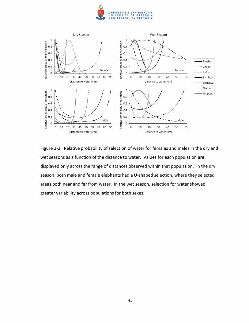
Figure 2-2. Relative probability of selection of water for females and males in the dry and

wet seasons as a function of the distance to water. Values for each population are

displayed only across the range of distances observed within that population. In the dry

season, both male and female elephants had a U-shaped selection, where they selected

areas both near and far from water. In the wet season, selection for water showed

greater variability across populations for both sexes.

44

Figure 2-3. Functional responses in habitat selection for female (red) and male (blue)

elephants. Selection coefficients were estimated for each individual using a resource

selection function model and were modelled as a function of the mean slope, tree cover,

or proximity to humans within each home range. Both significant (filled circle) and non-

significant (open circle) selection coefficients were modelled. Only the regression for

proximity to humans during the dry season was significant (P = 0.03).