CHAPTER 1 Introduction to the Theory of Incompressible Inviscid … · · 2010-11-241 CHAPTER 1...
140
1 CHAPTER 1 Introduction to the Theory of Incompressible Inviscid Flows * Thomas Y. Hou Applied and Computational Mathematics, Caltech, Pasadena, USA. E-mail: [email protected] Xinwei Yu Department of Mathematics, UCLA, Los Angeles, USA. E-mail: [email protected] Abstract In this chapter, we consider the 3D incompressible Euler equa- tions. We present classical and recent results on the issue of global existence/finite-time singularity. We also introduce the theories of lower dimensional model equations of the 3D Euler equations and the vortex patch problem. 1 Introduction The goal of these lecture notes is to introduce to the readers classical results as well as recent developments in the theory of 3D incompressible Euler equations. We will focus on the global existence/finite time singu- larity issue. We will start with the basic properties of the incompressible fluid flows, and then discuss the local and global well-posedness of the incompressible Euler equations. Of particular interest is the global ex- istence or possible finite time blow-up of the 3D incompressible Euler equation. This is one of the most outstanding open problems in the past century. Here, we carefully examine the nature of the nonlinear vor- tex stretching term for the 3D Euler equation as well as several model problems for the 3D Euler equation. We put extra effort in taking into account the local geometrical properties and possible depletion of nonlin- earity. By going through the nonlinear analysis of various fluid models, * The first author is partly supported by a NSF grant DMS-0713670 and a FRG grant DMS-0353838. The second author is partly supported by a NSF grant DMS- 0354488.
Transcript of CHAPTER 1 Introduction to the Theory of Incompressible Inviscid … · · 2010-11-241 CHAPTER 1...
1
CHAPTER 1
Introduction to the Theory ofIncompressible Inviscid Flows∗
Thomas Y. Hou
Applied and Computational Mathematics, Caltech,
Pasadena, USA.
E-mail: [email protected]
Xinwei Yu
Department of Mathematics, UCLA,
Los Angeles, USA.
E-mail: [email protected]
Abstract
In this chapter, we consider the 3D incompressible Euler equa-tions. We present classical and recent results on the issue of globalexistence/finite-time singularity. We also introduce the theoriesof lower dimensional model equations of the 3D Euler equationsand the vortex patch problem.
1 Introduction
The goal of these lecture notes is to introduce to the readers classicalresults as well as recent developments in the theory of 3D incompressibleEuler equations. We will focus on the global existence/finite time singu-larity issue. We will start with the basic properties of the incompressiblefluid flows, and then discuss the local and global well-posedness of theincompressible Euler equations. Of particular interest is the global ex-istence or possible finite time blow-up of the 3D incompressible Eulerequation. This is one of the most outstanding open problems in the pastcentury. Here, we carefully examine the nature of the nonlinear vor-tex stretching term for the 3D Euler equation as well as several modelproblems for the 3D Euler equation. We put extra effort in taking intoaccount the local geometrical properties and possible depletion of nonlin-earity. By going through the nonlinear analysis of various fluid models,
∗The first author is partly supported by a NSF grant DMS-0713670 and a FRG
grant DMS-0353838. The second author is partly supported by a NSF grant DMS-
0354488.
2 Thomas Y. Hou, Xinwei Yu
we can gain valuable insights into the fluid dynamic prolems being stud-ied. Through the analysis, we can also learn how various functionalanalysis and PDE techniques are being used for realistic applications,and what are their strengths and limitations. We especially emphasizethe interplay between the physical and geometric properties of the fluidflows and modern nonlinear PDE techniques. By going through theseanalyses systematically, we can have a good understanding of the stateof the art of nonlinear PDE methods and their applications to fluid dy-namics problems.
This chapter is organized as follows:
1. Introduction
2. Derivation and Exact Solutions
3. Local Well-posedness of the 3D Euler Equation
4. The BKM Blow-up Criterion
5. Recent Global Existence Results
6. Lower Dimensional Models for the 3D Euler Equation
7. Vortex Patch
2 Derivation and Exact Solutions
2.1 Derivation of the Euler Equations
The equation that governs the evolution of inviscid and incompressibleflow is the Euler equation. Here we first derive the 3D Euler equationbriefly. For more detailed derivations, the readers should consult othertext books in fluid mechanics, such as Chorin-Marsden [12], Lamb [31],Marchioro-Pulvirenti [36], or Lopes Filho-Nussenzveig Lopes-Zheng [33].
We consider a domain Ω which is filled with a fluid, such as water.In classical continuum mechanics, the fluid can be seen as consisting ofinfinitesimal particles. At each time t, each particle has a one to onecorrespondence to the coordinates x = (x1, x2, x3) ∈ Ω. The fluid canbe described by its density ρ, velocity u = (u1, u2, u3) and pressure p ateach such point x ∈ Ω. Under the above assumptions, we can denote theposition of any particle at time t by X(α, t) which starts at the positionα ∈ Ω at t = 0. Its evolution is governed by the following differentialequation:
dX(α, t)
dt= u(X(α, t), t),
X(α, 0) = α. (2.1)
Introduction to Incompressible Inviscid Flows 3
To study the dynamics of the fluid, we must establish relations betweenρ, u and p. We do this by considering two basic mechanical rules: theconservation of mass, and the conservation of momentum.
The conservation of mass claims that, for any fixed region W ⊆ Ωwhich doesn’t change with time,
d
dt
∫
W
ρ(x, t) dx = −∫
∂W
ρ(x, t)u(x, t) · n(x, t) dσ (2.2)
for all time t, where n(x, t) is the outer unit normal vector to ∂W , anddσ is the area unit on ∂W . Using the Gauss theorem we arrive at
d
dt
∫
W
ρ(x, t) dx = −∫
W
∇ · (ρ(x, t)u(x, t)) dx
which implies ∫
w
(ρt + ∇ · (ρu)) dx = 0.
If we assume the continuity of the integrand ρt + ∇ · (ρu), by the arbi-trariness of W , we get
ρt + ∇ · (ρu) = 0. (2.3)
Since otherwise, there would be a point x0 such that the integrand is not0. Without loss of generality, we assume (ρt + ∇ · (ρu)) (x0) > 0. Thenby continuity, there is r > 0 such that ρt + ∇ · (ρu) > 0 for any x ∈B(x0, r). This leads to a contradiction by taking we take W = B(x0, r).Equation (2.3) is called the continuity equation.
Let J be the determinant of the Jacobian matrix, ∂X∂α . It can ben
proved by direct calculations (the reader should try to prove this as anexercise, see also Chorin-Marsden [12]) that
dJ
dt= (∇ · u)J, J(0) = 1.
We assume that the flow is incompressible. Incompressibility impliesthat the flow is volume preserving. Using the above equation one canshow that the velocity is divergence-free, i.e.
∇ · u = 0 (2.4)
In this case, we have the determinant of the Jacobian matrix, J , to beidentically equal to one, i.e J ≡ 1. If the initial density is constant, i.e.ρ(x, 0) ≡ ρ0, equation (2.3) implies that density is constant globally, i.e.
ρ(x, t) ≡ ρ0.
Remark 2.1. -
4 Thomas Y. Hou, Xinwei Yu
1. The above derivation of the mass conservation equation is underthe assumption that ρ, u and ∂W are all smooth enough, e.g., C1.
2. One can also derive (2.3) in a Lagrangian way, i.e., by consideringan evolving region Ωt that is a collection of particles. See e.g.Lopes Filho-Nussenzveig Lopes-Zheng [33].
3. Yet another way is through the variational formulation. See e.g.Marchioro-Pulvirenti [36].
The conservation of momentum means
d
dt
∫
Ωt
ρu dx = F(Ωt) , (2.5)
where F(Ωt) is the force acting on Ωt. Here Ωt ≡ ∪α∈Ω0X(α, t) for
some Ω0 ⊆ Ω is a collection of particles that is carried by the flow. Wefirst assume that the interaction in the fluid is local, i.e., all the forcesbetween points inside Ωt cancel each other by Newton’s third law. Thisassumption implies
F(Ωt) =
∫
∂Ωt
f dσ
for some f . Our second assumption is that the fluid is ideal, whichmeans that f = −pn, where n is the unit outer normal to ∂Ωt. Now themomentum relation becomes
d
dt
∫
Ωt
ρu dx =
∫
∂Ωt
−pn dσ = −∫
Ωt
∇p dx ,
where the second equality follows from the Gauss theorem∫
Ω
∂if dx =
∫
∂Ω
fni dσ.
To derive a pointwise equation similar to (2.3), we need to put the ddt
inside the integration in the term
d
dt
∫
Ωt
ρu dx.
Note that since Ωt = X(Ω0, t) depends on t, it is not the same as
∫
Ωt
(ρu)t dx.
Instead of naıvely putting the differentiation inside, we proceed as fol-lows. We first change variables from the Eulerian variable x to the La-grangian variable α. Since the flow is incompressible, the determinant
Introduction to Incompressible Inviscid Flows 5
of the Jacobian matrix is equal to one, i.e., det(Xα) = 1. Thus we have
d
dt
∫
Ωt
ρu dx =d
dt
∫
Ω0
ρ(X(α, t), t)u(X(α, t), t) dα
=
∫
Ω0
d
dtρ(X, t)u(X, t) + ρ(X, t)
d
dtu(X, t) dα
=
∫
Ω0
(ρt + u · ∇ρ)u + ρ (ut + u · ∇u) dα
=
∫
Ω0
ρ(ut + u · ∇u) dα
=
∫
Ωt
ρ(ut + u · ∇u) dx.
where the first equality follows from the fact that the flow map α 7→X(α, t) is one-to-one and has Jacobian 1, and the fourth equality followsfrom (2.3) and the incompressibility condition. Now we have
∫
Ωt
ρ(ut + u · ∇u) dx = −∫
Ωt
∇p dx.
Finally, by the arbitrariness of Ωt, we get
ρ(ut + u · ∇u) = −∇p. (2.6)
by an argument that is similar to the one leading to (2.3). (2.6) is thebalance of momentum.
If we further assume that the flow has constant initial density, thenwe have ρ(x, t) ≡ ρ0, and equation (2.6) is equivalent to:
ut + u · ∇u = −∇p
where p is the ”rescaled” pressure p/ρ0.Under these assumptions, we obatin the 3D Euler equation as follows:
ut + u · ∇u = −∇p, (2.7)
∇ · u = 0.
In the remaining part of this lecture note, we will focus on (2.7).
6 Thomas Y. Hou, Xinwei Yu
2.2 The Vorticity-Stream function formulation
2.2.1 Vorticity
We consider the Taylor expansion of the velocity u(x, t) at some pointx.
u(x+ h, t) = u(x, t) + ∇u · h+O(h2)
= u(x, t) +∇u + ∇ut
2h+
∇u−∇ut
2h+O(h2)
≡ u(x, t) + S(x, t)h+ Ω(x, t)h+O(h2).
where S is symmetric and Ω is anti-symmetric. In 3D, it’s easy to seethat there is a vector ω such that
Ω(x, t)h =1
2ω(x, t) × h.
This implies that locally, the flow is rotating around an axis ξ(x, t) ≡ω(x,t)|ω(x,t)| . The vector field ω(x, t) is called “vorticity”. And it is easy to
check thatω(x, t) = ∇× u(x, t).
2.2.2 Vorticity-Stream function formulation
By taking ∇× on both sides of the 3D Euler equation (2.7), we have
ωt + u · ∇ω = ω · ∇u = S · ω. (2.8)
which is the vorticity formulation. The last equality follows from thefact that
Ω · ω =1
2ω × ω ≡ 0,
since by definition we have
1
2ω × h ≡ Ω · h
for any vector h. Now there are two unknowns ω and u, so we have tofind the relation between them to close the system. This relation is theso-called Biot-Savart law.
u(x) =1
4π
∫
R3
x− y
|x− y|3× ω(y) dy. (2.9)
Note that we need u(x) to vanish at ∞ for the above formula to hold.To derive the Biot-Savart law, first define a vector valued function Ψ,called “stream function”, such that
−4Ψ = ω.
Introduction to Incompressible Inviscid Flows 7
Now it is easy to check that
u = ∇× Ψ
satisfies∇× u = ω.
( Hint: Use the identity
−∇× (∇×) + ∇(∇·) = 4,
and then try to show‖∇ (∇ · Ψ)‖2
L2 = 0
using the same identity. Details are left as exercises. Or see Bertozzi-Majda [35]).
Now the Biot-Savart law (2.9) follows from the formula
Ψ =1
4π
∫1
|x− y|ω(y) dy,
where 14π
1|x| is the fundamental solution for the Poisson equation
−4u = f
in 3D.Besides (2.8), another important form of the vorticity evolution is
the “stretching formula”.
ω(X(α, t), t) = ∇αX(α, t)ω0(α) (2.10)
where ω0(α) = ω(X(α, 0), 0) = ω(α, 0), and X is defined by (2.1). Toprove it, just differentiate both sides with respect to time, which yields
ωt + u · ∇ω = ∇αu(X(α, t), t)ω0(α)
= ∇u · (∇αX · ω0)
= ∇u · ω(x, t),
which is just (2.8). One catch: this “proof” actually uses the uniquenessof the solution to the system (2.8), (2.9).
For the convenience of future references, we will denote the differ-entiation in time along the Lagrangian trajectory as D
Dt , which has theproperty:
D
Dtw = wt + u · ∇w.
DDt is also called material derivative.
8 Thomas Y. Hou, Xinwei Yu
2.2.3 2D Euler equations
In some physical cases, such as the flow passing around a cylinder withinfinite length, we can assume that u3 ≡ 0 and u, p depend on x1, x2
only. In this case, the Euler equations (2.7) remains the same form, butthe vorticity-stream function form reduces to
ωt + u · ∇ω = 0 (2.11)
and
u(x) =1
2π
∫(x− y)⊥
|x− y|2ω(y) dy (2.12)
where ω is a short-hand for ω3.
One important difference between 2D and 3D Euler equations is that,the right hand side is 0 in (2.11), which means the vorticity is conservedalong Lagrangian trajectory pathes. This point can be illustrated moreclearly by looking at the “stretching formula” in 2D, which is
ω(X(α, t), t) = ω0(α). (2.13)
This difference plays an important role in the theory of 2D Eulerequations, which is far more complete than its 3D counterpart.
2.3 Conserved Quantities
2.3.1 Local conserved quantities
First we consider those quantities that are carried by a collection of flowparticles.
Let C0 be a closed curve in R3. We define
Ct = ∪α∈C0X(α, t).
and the circulation
ΓCt ≡∮
Ct
u · ds.
Theorem 2.2. ( Kelvin’s Circulation Theorem ). ΓCt ≡ ΓC0.
Proof. We first prove the following.
d
dt
∫
Ct
u · ds =
∫
Ct
Du
Dt· ds.
Introduction to Incompressible Inviscid Flows 9
To prove it, let α(β) be a parametrization of the loop C0, with 0 ≤ β ≤ 1.Then Ct is parametrized as X(α(β), t). Thus
d
dt
∫
Ct
u · ds =d
dt
∫ 1
0
u(X(α(β), t), t) · ∂∂β
X(α(β), t) dβ
=
∫ 1
0
Du
Dt(X(α(β), t), t) · ∂
∂βX(α(β), t) dβ
+
∫ 1
0
u(X(α(β), t), t) · ∂∂β
u(X(α(β), t), t) dβ
where we have used the relation
∂X
∂t(α, t) = u(X(α, t), t).
Note that the first term is just∫
Ct
Du
Dt· ds,
we just need to show that the second term is 0. This is easy, since wehave ∫ 1
0
u · ∂∂β
u ds =1
2
∫ 1
0
∂
∂β(u · u) ds = 0,
which follows from the fact that Ct is a close loop.Now we prove the circulation theorem. We have
d
dt
∫
Ct
u · ds =
∫
Ct
Du
Dt· ds = −
∫
Ct
∇p · ds = −∫
Ct
psds = 0
since Ct is closed. Thus ends the proof.
Next let C0 be a general curve and Ct = X(C0, t). Then as long asthe flow is still regular, Ct is still a curve in R3. Ct is called a vortexline if the following is satisfied
C0 is tangent to ω0(α) at any α ∈ C0. (2.14)
One can verify that as long as (2.14) is satisfied, the same tangencycondition is satisfied at every moment t, i.e.,
Ct is tangent to ω(x, t) at any x ∈ Ct.
A collection of vortex lines is called a “vortex tube”. One readilysees that vorticity is always tangent to the side surface of a vortex tube.
The above properties make vortex tube/line very important objectsin the theories/numerical simulations/physical experiments of the 3DEuler equation, as we will reveal later in this lecture note.
10 Thomas Y. Hou, Xinwei Yu
2.3.2 Global conserved quantities
The most well-known global conserved quantities are the following (we will indicate the dimension and region/manifold, Td stands for d-dimensional periodic torus):
1. The integral of velocity. ( Rd and Td , d = 2, 3 ).
d
dt
∫u dx = 0.
2. Kinetic energy. ( Rd, Td, smooth bounded domain, d = 2, 3 ).
d
dt
∫|u|2 dx = 0.
Remark 2.3. In the Rd case, caution must be taken. We actuallyneed that the kinetic energy
∫|u|2 dx to be finite. In 3D this
requirement is reasonable, while in 2D it is not.
3. Center of vorticity. ( R2 , if uω decays fast enough at ∞ ).
x =
∫
R2
xω dx = const.
4. Moment of inertia. ( R2 , if uω decays fast enough at ∞).
I =
∫
R2
|x|2 ω dx = const.
5. Functions of vorticity. ( d = 2 ).
∫
Ωt
f(ω) dx =
∫
Ω0
f(ω0) dα
for any measurable f and material domain Ωt. In particular, wesee that the Lp norm of ω is conserved for 1 ≤ p ≤ ∞.
6. Other quantities. ∫
R3
x× ω dx
∫
R3
x× (x× ω) dx;
helicity ∫
R3
u · ω dx;
and spiralityω · γ
Introduction to Incompressible Inviscid Flows 11
where γ = u + ∇φ with φ solving
D
Dtφ = − |u|2 /2 + p.
This quantity is conserved along particle trajectories.
2.4 Special Flows
2.4.1 Axisymmetric Flow
In this subsection we introduce the axisymmetric flow, i.e., when writtenin cylindrical coordinates x1 = r cos θ, x2 = r sin θ and x3 = z, thevelocity u and the pressure p depend only on r and z. Unlike the 2DEuler equations, this particular flow retains some 3D characters and isoften referred to as the 2 1
2 -D equations.We introduce the cylindrical frame of reference:
er = (cos θ, sin θ, 0)
eθ = (− sin θ, cos θ, 0)
ez = (0, 0, 1).
and can easily rewrite the 3D Euler equations in the new frame, withu = u(r, z) and p = p(r, z), as
ut + (u · ∇)u +B = −∇p (2.15)
where∇ = (∂r , 0, ∂z)
and
B =uθ
r(−uθ, ur, 0).
We leave the details (which can be found in e.g. Lopes Filho-NussenzveigLopes-Zheng [33]) for this system to the reader as exercises.
1. Derive equations (2.15).
2. Prove that, in the moving frame (er, eθ, ez), we have
ω = ωrer + ωθeθ + ωzez
≡(−∂zu
θ)er + (∂zu
r − ∂ruz) eθ +
(∂ru
θ +uθ
r
)ez.
3. When uθ ≡ 0, (2.15) becomes axisymmetric flows without swirl.Prove that the equations are
(∂t + u · ∇
)u = −∇p
∇ · (ru) = 0 (2.16)
12 Thomas Y. Hou, Xinwei Yu
Furthermore, one can reduce the equation into the r−z plane whichis 2D. Prove that the equation for ωθ ( note that ωr = ωz = 0 ) is
(∂t + u · ∇)
(ωθ
r
)= 0.
2.4.2 Radially ( circularly ) symmetric flow
In the 2D case. We consider ω0 ≡ ω0(r) which is circularly symmetric.Then by exploring the invariance of the Laplacian we easily see that ψdefined by
−4ψ = ω0
is also a circularly symmetric function. Thus
u = ∇⊥ψ
is always tangent to the contours ω0 ≡const. One can easily verify that
ω ≡ ω0,u ≡ u0
is a steady solution for the 2D Euler equations. The velocity is explicitlygiven as
u =x⊥
r2
∫ r
0
sω(s) ds, (2.17)
where r = |x|. These stationary solutions are called Rankine vortices.The reader can try to derive the “radial symmetric biot savart law”(2.17) as an exercise (Hint: it is easier to start from the stream functionΨ).
Now consider the special case, where ω0 is supported inBR ≡ x | |x| ≤ R,with
∫BR
ω0 = 0. Then it is easy to see that u is also supported in BR.Such a vortex is called a confined eddy. The importance of this observa-tion can be seen from the following property:
The superposition of two disjoint confined eddies is still a solution.
This gives us a way to construct very complicated exact solutions to the2D Euler equations.
2.4.3 Jets and Strains
LetD(t) be any family of symmetric and trace-free matrices that smoothlydepends on t, and let ω solves
dω
dt= D(t)ω
ω(0) = ω0.
Introduction to Incompressible Inviscid Flows 13
We introduce
u =1
2ω × x+D(t)x.
It is easy to check that we can define p such that u solves the 3D Eulerequations in the whole space. One thing that worths noting is that,the velocity we defined above is growing unboundedly at ∞ and is thusnon-physical.
It is illustrating to study some special cases.
1. Jet. Take ω0 = 0 thus ω ≡ 0. Note that we can write D(t) to bediagonal:
D(t) =
−γ1 0 00 −γ2 00 0 γ1 + γ2
and getu = (−γ1x1,−γ2x2, (γ1 + γ2)x3).
2. Swirling jet. We take ω0 = (0, 0, a) and get
ω = (0, 0, ae(γ1+γ2)t),
and
u =
(−γ1x1 −
1
2a(t)x2,−γ2x2 +
1
2a(t)x1, (γ1 + γ2) x3
).
3. Strain. We take ω0 = 0 and γ1 = −γ2 = γ.
u = (−γx1, γx2, 0) .
3 Local Well-Posedness of the 3D Euler Equa-tion
First we consider the local well-posedness for classical solutions. Byclassical solutions we mean solutions such that (2.7) holds in the classicalsense, i.e., all the derivatives are in the classical sense, the multiplicationsare pointwise, and the equalities hold everywhere. Our main goal in thissection is to prove the following:
Theorem 3.1. If the initial velocity u0 ∈ Hm∩C2 for some m > 2+d/2,then there is T > 0 such that there is a unique solution u ∈ Hm ∩C2 in[0, T ].
To do this, we use the standard technique of mollifiers. In short, weapproximate (2.7) by a sequence of equations that can be shown to admitglobal smooth solutions, and then establish the local in time existenceby taking limit.
14 Thomas Y. Hou, Xinwei Yu
3.1 Analytical preparations
3.1.1 Sobolev spaces
The Sobolev spaces Hk, k ∈ Z, k ≥ 0 is defined as
Hk(Rd) =
f(x) |
∑
|α|≤k
‖∂αf‖2L2 <∞
where α is a multi-index α = (α1, α2, . . . , αd). |α| ≡∑αi and ∂α ≡
∂|α|
∂xα1
1···∂x
αdd
. Hk is a Banach space with norm
‖f‖Hk =
∑
|α|≤k
‖∂αf‖2L2
1/2
.
If we consider the Fourier transform of f , we have
‖f‖Hk =
∑
|α|≤k
∥∥∥ξαf∥∥∥
2
L2
1/2
where ξα ≡ ξα1
1 · · · ξαd
d . Now by some simple algebra we can obtain thefollowing equivalent norm
‖f‖Hk ∼∥∥∥〈ξ〉k f
∥∥∥L2
∼∥∥∥(1 −4)
k/2f∥∥∥
L2
where 〈ξ〉 ≡ (1 + |ξ|2)1/2, and 4 is the Laplacian.The point in writing the Hk norm this way is that, now we can take
k to be any real number instead of non-negative integers. Usually, whenk is not an integer, we replace it by s.
The following theorem is used extensively in PDE researches.
Theorem 3.2. The space C∞0 (Rd) is dense in Hs(Rd).
The most important property of the Sobolev spaces is the embeddingtheorems. We will not prove these theorems here, interested readers canlook up the proof in e.g. Adams [1], which is a classic and not very hardto read.
Before introducing the theorems, we first recall what “embedding”means. Consider two Banach spaces X and Y , with norms ‖·‖X and‖·‖Y . Assume that there is a third space Z which is dense in both Xand Y . We say X is embedded in Y , if there is a constant C such that
‖·‖Y ≤ C ‖·‖X .
Introduction to Incompressible Inviscid Flows 15
This means that all the elements in X is also in Y . Furthermore, we sayX is compactly embedded in Y , if X is embedded in Y , and any boundedsubset of X ( in the X norm ) is precompact in Y ( with respect to theY norm ). That is, if xn ⊂ X is uniformly bounded, then there is asubsequence which is Cauchy in Y . We denote embedding by →.
Theorem 3.3. (Embeddings for Hs). Let Hs(Rd) be the Sobolev space.We have
Hs+k → Ck
for all s > d/2 and k ∈ Z, nonnegative.
3.1.2 Hodge decomposition and the Leray projection
We denote by Hs(Rd) the Sobolev spaces, and let V s ⊂ Hs(Rd; Rd) bethe subspace of divergence-free vector fields.
Lemma 3.4. ( Hodge decomposition ). Let u be a vector field withcomponents in L2(Rd). There exists a unique decomposition u = u1+u2,where u1 is divergence-free and u2 is a gradient. Furthermore u1 and u2
are orthogonal in L2. We denote by P the projection L2(Rd; Rd) 7→ V 0
which maps u to u1, then P commutes with derivatives, convolution andis also a map from Hs to V s.
Proof. First we solve
4φ = ∇ · u
Thus
φ = 4−1(∇ · u) +H
where H is a harmonic function and 4−1 is the convolution with theGreen’s function of the Laplacian in Rd. Now define
u2 = ∇φ = (∇24−1) · u + ∇H
By going to the Fourier space, it is easy to see that the first term is inL2. To make u2 ∈ L2, we must have ∇H ∈ L2, which means it mustvanish at ∞. But since each entry of ∇H is harmonic, we see that thisimplies that ∇H ≡ 0.
Now we have
P =(I −∇24−1
)· . (3.1)
It is easy to check the commutativity properties.
This operator P is often referred to as the Leray projection operator.
16 Thomas Y. Hou, Xinwei Yu
3.1.3 The Aubin-Lions Lemma
For evolution PDEs, generally one can not treat time and space as equal,so one need compactness results that has different requirement in spaceand time. A standard result is the Aubin-Lions lemma.
First we prove a technical lemma. Let X → Y → Z be Banachspaces that have embedding relations as indicated. Recall that X → Yis compact means that for any fn that is uniformly bounded in X ,there is a subsequence that is convergent in the norm of Y .
Lemma 3.5. Assume that X → Y is compact. then for every η > 0there exists a constant Cη > 0 such that
‖v‖Y ≤ η ‖v‖X + Cη ‖v‖Z
for every v ∈ X.
Proof. The proof is standard. We prove by contradiction. Assume thereis a η > 0 and a sequence vn ⊂ X such that
‖vn‖Y > η ‖vn‖X + n ‖vn‖Z ,
then by taking wn ≡ vn/ ‖vn‖X we see that the same inequality holdsfor wn. Now wn is bounded in X , which means there is a subsequence,still denote as wn, such that
wn → w ∈ Y
in Y . Note that ‖wn‖Y ≤ C‖wn‖X ≤ C by the embedding assumptionand the fact that ‖wn‖X = 1. Now divide both sides of the equation forwn by n, we have
wn → 0 in Z.
But on the other hand, we have
wn → w 6= 0
in Y and thus we have a contradiction, since the embedding, convergencein Y to some limit implies convergence in Z to the same limit.
Lemma 3.6. ( Aubin-Lions ). Suppose that X → Y is compact. LetT > 0. Let un be a bounded sequence in L∞ ([0, T ] ;X). Suppose thissequence is equicontinuous as Z-valued functions defined on [0, T ]. Thenthe same sequence is precompact in C ([0, T ] ;Y ).
Proof. First, it follows directly from Lemma 3.5 that each un is inC ([0, T ] ;Y ). Second, by the conditions in the Lemma we see that wecan use the Arzela-Ascoli lemma on C ([0, T ] ;Z) and see that un is pre-compact in it. Finally, still by Lemma 3.5 we see that un is precompactin C ([0, T ] , Y ).
Introduction to Incompressible Inviscid Flows 17
Remark 3.7. A comparison with the Arzela-Ascoli lemma in analysis ishelpful. There we basically have a sequence that is uniformly boundedand equicontinuous in C ([0, T ] , Y ) for some Y . Here the boundednesscondition, which is usually easier to establish, is strengthened, while theharder condition equicontinuity is weakened.
3.1.4 Calculus Inequalities
Let u and v be in Hm(Rd) with m ∈ N.
Lemma 3.8. -
1. If u and v are bounded and continuous then there exists a constantC > 0 such that
‖uv‖Hm ≤ C (‖u‖L∞ ‖Dmv‖L2 + ‖v‖L∞ ‖Dmu‖L2) .
2. If u, v and ∇u are bounded and continuous then there exists a con-stant C > 0 such that∑
0≤|α|≤m
‖Dα (uv) − uDαv‖L2 ≤ C(‖∇u‖L∞
∥∥Dm−1v∥∥
L2+ ‖v‖L∞ ‖Dmu‖L2
).
Proof. First we prove 1. It is enough to prove that∥∥DαuDβv
∥∥L2
≤ C (‖u‖L∞ ‖Dmv‖L2 + ‖v‖L∞ ‖Dmu‖L2)
where in the RHS (right hand side) we actually define
‖Dmv‖2L2 =
∑
|α|=m
‖Dαv‖2L2 ,
while in the LHS (left hand side) α, β are multi-indices with |α|+|β| = m.We illustrate the idea of the proof by considering the scalar case. We
estimate
‖u′v′‖L2 =
(∫(u′v′)
2dx
)1/2
where α = β = 1 and m = 2. By Holder’s inequality, we have
‖u′v′‖L2 ≤ ‖u′‖L4 ‖v′‖L4 .
Next we establish the Gagliardo-Nirenberg inequality
∥∥Diu∥∥
L2r/i ≤ cr ‖u‖1−i/rL∞ ‖Dru‖i/r
0
with 0 ≤ i ≤ r. In our case, i = 1, r = 2, the Gagliardo-Nirenberginequality reduces to
‖u′‖L4 ≤ c ‖u‖1/2L∞ ‖u′′‖1/2
0 . (3.2)
18 Thomas Y. Hou, Xinwei Yu
The proof is easy. We have
‖u′‖4L4 =
∫(u′)
4dx
=
∫(u′)
3du
≤ c
∣∣∣∣∫u (u′)
2u′′ dx
∣∣∣∣
≤ c
∣∣∣∣∫u2 (u′′)
2dx
∣∣∣∣1/2 ∣∣∣∣
∫(u′)
4dx
∣∣∣∣1/2
≤ c ‖u‖L∞ ‖u′′‖L2 ‖u′‖2L4 .
which proves (3.2).Now we have
‖u′v′‖L2 ≤ c ‖u‖1/2L∞ ‖u′′‖1/2
L2 ‖v‖1/2L∞ ‖v′′‖1/2
L2 .
By using Young’s inequality
ab ≤ ap
p+bq
q
where p, q > 0 with 1p + 1
q = 1 we finish the proof.The general cases of 1 and 2 are left as exercises.
3.1.5 Gronwall’s inequality
In dealing with evolution equations, we need to estimate various quan-tities. In doing so we often end up with inequalities like
X(t) ≤ a(t) +
∫ t
0
b(s)X(s) ds
whereX(t) is the non-negative quantity we need to estimate, and a(t), b(t) ≥0 with a(t) differentiable. The trick in getting an estimate for X is thefollowing. We also assume that everything is continuous.
Fix ε > 0, let Y ε(t) satisfy
Y ε(t) = a(t) + ε+
∫ t
0
b(s)Y ε(s) ds,
then it is easy to see that Y ε(t) is differentiable, and satisfies
(Y ε)′ (t) = a′(t) + b(t)Y ε(t)
Y ε(0) = a(0) + ε
Introduction to Incompressible Inviscid Flows 19
which gives
Y ε(t) = (a(0) + ε) e t0
b(s) ds +
∫ t
0
a′(s)e t
sb(τ) dτ ds.
Now by arbitrariness of ε we get what we need, as long as we have
X(t) ≤ Y ε(t)
for any ε > 0. To show this, consider W ≡ Y ε −X , which satisfies
W (t) ≥ ε+
∫ t
0
b(s)W (s) ds
W (0) = ε > 0.
By the continuity of W and the condition b(s) ≥ 0 it is easy to see thatW (t) ≥ ε for all t > 0. Thus we proved the following lemma.
Lemma 3.9. ( Gronwall’s lemma. ) If X(t), a(t), b(t) ≥ 0 are continu-ous, a(t) differentiable, with
X(t) ≤ a(t) +
∫ t
0
b(s)X(s) ds,
then we can estimate X(t) by
X(t) ≤ a(0)e
t0
b(s) ds +
∫ t
0
a′(s)e
ts
b(τ) dτ ds.
3.2 Properties of mollifiers
Definition 3.10. Let ρ ∈ C∞0 (Rd) be any radial function, i.e., ρ(x)
depends only on |x|. We choose ρ ≥ 0 with∫
Rd ρ dx = 1. For any ε > 0,define
ρε(x) = ε−dρ(x/ε).
Then we call the family ρε a family of mollifiers.In the following, we will denote
M εf = (ρε ∗ f) (x).
for any function f .
Next we develop some main properties of the mollification operatorM ε.
Lemma 3.11. . For any function f such that M εf is well-defined, wehave
20 Thomas Y. Hou, Xinwei Yu
1. M εf is smooth, i.e., C∞.
2. For all f ∈ C0(Rd), we have M εf → f uniformly on any compactset Ω, and
‖M εf‖L∞ ≤ ‖f‖L∞ .
3. M εDα = DαM ε for any multi-index α.
4. For all f ∈ Lp, g ∈ Lq with 1/p+ 1/q = 1,
∫
Rd
(M εf) g dx =
∫
Rd
f (M εg) dx.
5. For all f ∈ Hs(Rd), M εf converges to f in Hs and the rate ofconvergence in the Hs−1 norm is O(ε).
6. For all f ∈ Hs(Rd), k ∈ Z+ ∪ 0, and ε > 0, we have
‖M εf‖s+k ≤ csk
εk‖f‖s ,
∥∥M εDkf∥∥
L∞ ≤ ckεd/2+k
‖f‖L2 .
Proof. 1–4 are easy and omitted. Interested readers can try to provethem or check Bertozzi-Majda [35]. To prove 5 and 6, it is important toknow the representation of M ε in the Fourier space:
M εf(ξ) = ρ(εξ)f(ξ).
Note that by construction
ρ(0) =
∫ρ dx = 1.
As ε→ 0, for any ξ, we have
ρ(εξ) ∼ 1 +O(ε).
It is clear now that why we can expect M εf → f at all.Another key factor in proving 5 and 6 is the Fourier side characteri-
zation of Hs(Rd). Recall that
∣∣∣∇f(ξ)∣∣∣ = c |ξ|
∣∣∣f(ξ)∣∣∣
where c depends on the definition of Fourier transforms, e.g., if we define
f(ξ) =
∫e−iξ·xf(x) dx
Introduction to Incompressible Inviscid Flows 21
then c = 1. The particular value of c is not important here. In thefollowing, we will just take c = 1. Now f ∈ Hs is equivalent to
〈ξ〉s f(ξ) ∈ L2
where 〈ξ〉 ≡(1 + |ξ|2
)1/2
.
With the above understanding, 5 and 6 are easy to prove. For ex-ample, we prove the second estimate in 6. For any multi-index α with|α| = k, we have
|(M εDαf) (x)| = c
∣∣∣∣∫eiξ·xρ(εξ)ξαf(ξ) dξ
∣∣∣∣
≤ c
∫
Rd
|ρ(εξ)| |ξ|k∣∣∣f(ξ)
∣∣∣ dξ
. ‖f‖L2
(∫
Rd
|ρ(εξ)|2 |ξ|2kdξ
)1/2
= ‖f‖L2
(∫
Rd
|ρ(η)|2 |η|2kdη
)1/2
ε−k−d/2
. ε−k−d/2 ‖f‖L2
where η ≡ εξ and note that the integration is over Rd, thus the factorε−d/2. The integral on ρ is bounded since ρ ∈ C∞
0 ⊂ Hk is a fixedfunction.
The other inequalities in 5 and 6 can be proved similarly and are leftto the readers.
3.3 Global existence of the mollified equation
We consider the mollified equations:
∂tuε +M ε (((M εuε) · ∇) (M εuε)) = −∇pε
∇ · uε = 0
uε(x, 0) = u0(x). (3.3)
or, by using the Leray projection operator,
∂tuε + P (M ε (((M εuε) · ∇) (M εuε))) = 0,
Puε = uε,
uε(x, 0) = u0(x). (3.4)
where uε denotes the solution and is not necessarily of the form M εv forsome v. We will prove the global existence ( i.e., for all time t ∈ R+) of
22 Thomas Y. Hou, Xinwei Yu
the mollified 3D Euler equations. Our strategy is to prove local existenceby treating (3.4) as an ODE in some Banach space, and then extend theexistence time to ∞. In the following of this section, we will omit thesuperscipt ε and denote uε by u.
Lemma 3.12. Let m ∈ N. Then for every u0 ∈ V m and ε > 0 thereexists T ε > 0 and a solution uε ∈ C1 ([0, T ε) ;V m) to the problem (3.4),or equivalently, (3.3).
Proof. Let
Fε(u) = −P (M ε (((M εu) · ∇) (M εu))) .
Then (3.4) becomesduε
dt= Fε(u
ε).
which is an ODE in a Banach space. The only thing we need to checkbefore applying the Picard iteration to get local in time existence is that
1. Fε : Vm 7→ Vm, and
2. Fε is locally Lipschitz in V m.
For the first claim, we have the following estimate:
‖Fε(u)‖Hm ≤ ‖M ε (((M εu) · ∇) (M εu))‖Hm
≤ C ‖M ε (∇ · (M εu⊗M εu))‖Hm
≤ C
ε‖M εu⊗M εu‖Hm
≤ C
ε3/2‖u‖2
Hm
where we have used the calculus inequalities (see Lemma 2.1.8) andthe following properties of the mollifiers: ‖M εDf‖Hm ≤ C ‖f‖Hm /ε ,‖M εu‖L∞ ≤ C ‖u‖Hm /εd/2, which follows from Lemma 2.1.11(6).
Next we show that Fε is Lipschitz. Let v1 and v2 belong to V m, then
‖Fε(v1) − Fε(v2)‖Hm ≤ C
ε(‖M εv1 ⊗M ε (v1 − v2)‖Hm + ‖M εv2 ⊗M ε (v1 − v2)‖Hm)
by adding and subtracting M ε (((M εv1) · ∇) (M εv2)). By using the cal-culus inequality again (Lemma 2.1.8), we can bound the RHS by
C
ε3/2(‖v1‖Hm + ‖v2‖Hm ) ‖v1 − v2‖Hm ≤ Cε ‖v1 − v2‖Hm
since ‖vi‖Hm (i=1,2) is bounded and ε is finite. This proves the localLipschitz condition of Fε.
Introduction to Incompressible Inviscid Flows 23
To extend the existence time to infinity we need to show that theLipschitz constant
C
ε3/2(‖v1‖Hm + ‖v2‖Hm)
depends only on ε and initial conditions. We only need to show that forany solution u, ‖u‖Hm is bounded by the Hm norm of the initial valueu0.
First, by integration by parts, it is easy to see that
‖u‖L2 ≤ ‖u0‖L2 .
The remaining is done by the following lemma:
Lemma 3.13. Let m ∈ N and u ∈ C1 ([0, T ) ;V m) be a solution of themollified 3D Euler equations (3.4). Then
‖u‖Hm ≤ ‖u0‖Hm eC t0‖∇Mεu‖L∞ dt
Proof. Let α be a multi-index, with |α| ≤ m. Applying Dα to both sidesof (3.3), multiplying them by Dαu and integrate, we have
1
2
d
dt
∫|Dαu|2 dx = −
∫Dαu · (M εDα (((M εu) · ∇) (M εu)))
= −∫DαM εu ·Dα (((M εu) · ∇) (M εu)) dx
= −∫DαM εu ·Dα (((M εu) · ∇) (M εu))
+
∫DαM εu · (((M εu) · ∇)DαM εu) dx,
where the term involving the pressure vanishes after integrated by partsdue to the incompressibility condition, and the last equality comes fromthe following argument:∫DαM εu·(((M εu) · ∇)DαM εu) dx =
1
2
∫(M εu)·∇
(|DαM εu|2
)dx = 0
via integration by parts due to the incompressibility condition.Now we sum over all 0 ≤ |α| ≤ m. Using the calculus inequality, we
have
d
dt‖u‖2
Hm ≤ C ‖u‖Hm
∑
|α|≤m
‖Dα (((M εu) · ∇) (M εu)) − ((M εu) · ∇)DαM εu‖L2
≤ C ‖u‖Hm
(‖∇M εu‖L∞
∥∥Dm−1DM εu∥∥
L2+ ‖DmM εu‖L2 ‖∇M εu‖L∞
)
≤ C ‖∇M εu‖L∞ ‖u‖2Hm .
To finish the proof, we just need to apply the standard Gronwall’s in-equality from Lemma 3.9.
24 Thomas Y. Hou, Xinwei Yu
3.4 Local existence of the Euler equations
Now we are ready to give the local existence theorem.
Theorem 3.14. Let u0 ∈ V m for m ≥ 4. There exists T0 = T0 (‖u0‖Hm) >0 such that for any T < T0, there exists a unique solution u ∈ C1 ([0, T ] ;V m)of the 3D incompressible Euler equations with u0 as initial data.
Proof. By Lemma 3.13 we have
d
dt‖uε‖2
Hm ≤ C ‖∇M εuε‖L∞ ‖uε‖2Hm
Note that m ≥ 4 > 3/2 + 1, by Theorem 3.3, Hm is embedded into C1,which means ‖∇M εuε‖L∞ ≤ ‖M εuε‖C1 . ‖M εuε‖Hm ≤ ‖uε‖Hm . Thuswe have
d
dt‖uε‖Hm ≤ C ‖uε‖2
Hm
and the constant C here is independent of ε. Therefore we see that ouruε is uniformly bounded in L∞ ([0, T ] ;Hm) by
‖u0‖Hm
1 − CT ‖u0‖Hm
.
for any T < T0 ≡ (C ‖u0‖Hm)−1. To apply the Lions-Aubin lemma weneed to show that uε is Lipschitz in t in some larger space, which wetake to be Hm−1. In fact we have
‖∂tu‖Hm−1 = ‖Fε(uε)‖Hm−1
≤ C ‖∇ · (M εuε ⊗M εuε)‖Hm−1
≤ C ‖M εuε ⊗M εuε‖Hm
≤ C ‖M εuε‖L∞ ‖uε‖Hm
≤ C ‖uε‖2Hm ,
where we have used the calculus inequality (Lemma 2.1.8) and the Sobolevembedding theorem. Thus we see that uε is Lipschitz in t wrt Hm−1-norm.
We fix Rk > 0 and use Lemma 3.6 ( The reason we need this stepis that we need Hm → Hm−1 to be compact, which won’t hold forunbounded regions, as can be seen by taking X = H1(R), Y = L2(R)and fn(x) = f(x − n) for some f ∈ H1. Obviously fn is boundedin X but not convergent in Y . ) with X = Hm(B(0, Rk)), Y =Z = Hm−1(B(0, Rk)). Taking Rk → ∞ and using a diagonal argu-ment we see that uε has a subsequence, which we do not relabel, thatis strongly convergent in C
([0, T ] ;Hm−1
loc (R3)). Denote the limit by u.
Introduction to Incompressible Inviscid Flows 25
Moreover, since m ≥ 4 > 3/2+2, we see that the convergence also holdsin C
([0, T ] ;C1
loc(R3)).
We rewrite the equation as
uε = u0 +
∫ t
0
F ε(uε) ds.
It is easy to see that
u = u0 +
∫ t
0
F (u) ds
where F (u) ≡ P (u · ∇u). Thus we have further that
u ∈ C1([0, T ] ;C1
loc(R3))
which implies that we can legitimately differentiate with respect to t.Now taking d/dt on both side, we see that u satisfies
ut + P (u · ∇u) = 0
∇ · u = 0
u(·, 0) = u0
|u| → 0 as |x| → ∞.
The final step for existence is to recover the pressure. This followsdirectly from the Leray decomposition.
Now we show the uniqueness. Suppose that there are two solutionsu1 and u2, then we immediately have
(u1 − u2)t + P (u1 · ∇u1 − u2 · ∇u2) = 0
with u1 − u2 = 0 at t = 0. Multiply to u1 − u2 and integrate, we caneasily derive
d
dt‖u1 − u2‖2
L2 ≤ C(‖u1‖Hm + ‖u2‖Hm) ‖u1 − u2‖2L2
by the calculus inequalities. Then by using Gronwall’s inequality, wesee that the only solution is u1 − u2 ≡ 0. Thus ends the proof foruniqueness.
4 The BKM Blow-up Criterion
4.1 The Beale-Kato-Majda Criterion
One of the important points that should be noted is that the aboveexistence result is local in time, meaning that the solution may cease to
26 Thomas Y. Hou, Xinwei Yu
be in Hm (also known as (aka) blow-up ) in some finite time. Thus itis important to have some quantities to indicate such a blow-up. One ofthem is the quantity ∫ T
0
‖ω(·, s)‖L∞ ds
proposed by T. Beale, T. Kato and A. Majda.By the same method used in the last section, we can have the follow-
ing bound:
‖u(·, t)‖Hm ≤ Cec
t0‖∇u‖L∞ ds ‖u0‖Hm .
So it is clear that as long as ‖∇u‖L∞ is uniformly bounded in some timeinterval (0, T ), then the solution exists upto T . In fact this is what Ebin,Fischer and Marsden proved in their 1972 paper [23]. Thus the key is tobound ‖∇u‖L∞ by ‖ω‖L∞ at the same time t. Recall the 3D Biot-Savartlaw
u(x) =
∫K(x− y)ω(y) dy
where K(z) is the matrix kernel
K(z) =1
|z|3
0 −z3 z2z3 0 −z1−z2 z1 0
.
If we differentiate under the integration formally, we would have
∇u(x) =
∫∇K(x− y)ω(y) dy. (4.1)
The operator ∇K∗ in fact has nice properties. To see this, we recalla theorem from Stein [44], which is also called the Calderon-ZygmundLemma.
Theorem 4.1. Let K ∈ L2(Rd). We suppose:
1. The Fourier transform of K is essentially bounded
∣∣∣K(x)∣∣∣ ≤ B.
2. K is C1 outside the origin and
|∇K(x)| ≤ B/ |x|d+1.
For f ∈ L1 ∩ Lp, let us set
(Tf)(x) =
∫
Rd
K(x− y)f(y) dy.
Introduction to Incompressible Inviscid Flows 27
Then there exists a constant Ap, so that
‖T (f)‖p ≤ Ap ‖f‖p , 1 < p <∞.
One can thus extend T to all of Lp by continuity. The constant Ap
depends only on p,B, and the dimension n. In particular, it does notdepend on the L2 norm of K.
The remark following the theorem in Stein [44] claims that the as-sumption K ∈ L2 can be safely dropped in practice.
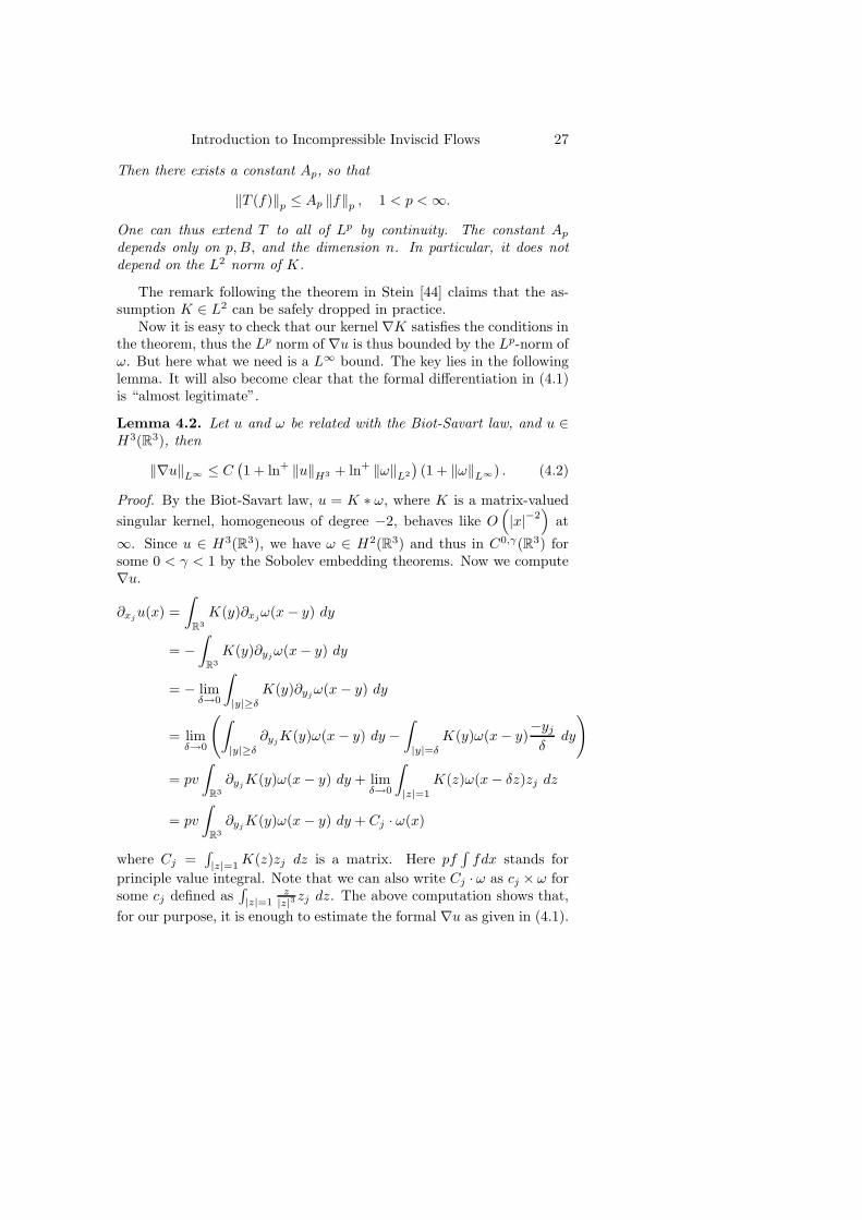
Now it is easy to check that our kernel ∇K satisfies the conditions inthe theorem, thus the Lp norm of ∇u is thus bounded by the Lp-norm ofω. But here what we need is a L∞ bound. The key lies in the followinglemma. It will also become clear that the formal differentiation in (4.1)is “almost legitimate”.
Lemma 4.2. Let u and ω be related with the Biot-Savart law, and u ∈H3(R3), then
‖∇u‖L∞ ≤ C(1 + ln+ ‖u‖H3 + ln+ ‖ω‖L2
)(1 + ‖ω‖L∞) . (4.2)
Proof. By the Biot-Savart law, u = K ∗ ω, where K is a matrix-valued
singular kernel, homogeneous of degree −2, behaves like O(|x|−2
)at
∞. Since u ∈ H3(R3), we have ω ∈ H2(R3) and thus in C0,γ(R3) forsome 0 < γ < 1 by the Sobolev embedding theorems. Now we compute∇u.
∂xju(x) =
∫
R3
K(y)∂xjω(x− y) dy
= −∫
R3
K(y)∂yjω(x− y) dy
= − limδ→0
∫
|y|≥δ
K(y)∂yjω(x− y) dy
= limδ→0
(∫
|y|≥δ
∂yjK(y)ω(x− y) dy −∫
|y|=δ
K(y)ω(x− y)−yj
δdy
)
= pv
∫
R3
∂yjK(y)ω(x− y) dy + limδ→0
∫
|z|=1
K(z)ω(x− δz)zj dz
= pv
∫
R3
∂yjK(y)ω(x− y) dy + Cj · ω(x)
where Cj =∫|z|=1
K(z)zj dz is a matrix. Here pf∫fdx stands for
principle value integral. Note that we can also write Cj · ω as cj × ω forsome cj defined as
∫|z|=1
z|z|3
zj dz. The above computation shows that,
for our purpose, it is enough to estimate the formal ∇u as given in (4.1).
28 Thomas Y. Hou, Xinwei Yu
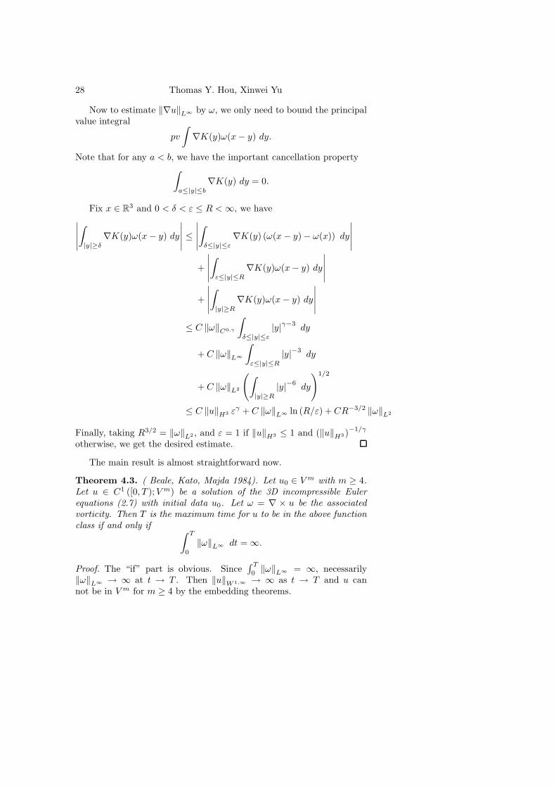
Now to estimate ‖∇u‖L∞ by ω, we only need to bound the principalvalue integral
pv
∫∇K(y)ω(x− y) dy.
Note that for any a < b, we have the important cancellation property∫
a≤|y|≤b
∇K(y) dy = 0.
Fix x ∈ R3 and 0 < δ < ε ≤ R <∞, we have∣∣∣∣∣
∫
|y|≥δ
∇K(y)ω(x− y) dy
∣∣∣∣∣ ≤∣∣∣∣∣
∫
δ≤|y|≤ε
∇K(y) (ω(x− y) − ω(x)) dy
∣∣∣∣∣
+
∣∣∣∣∣
∫
ε≤|y|≤R
∇K(y)ω(x− y) dy
∣∣∣∣∣
+
∣∣∣∣∣
∫
|y|≥R
∇K(y)ω(x− y) dy
∣∣∣∣∣
≤ C ‖ω‖C0,γ
∫
δ≤|y|≤ε
|y|γ−3dy
+ C ‖ω‖L∞
∫
ε≤|y|≤R
|y|−3 dy
+ C ‖ω‖L2
(∫
|y|≥R
|y|−6dy
)1/2
≤ C ‖u‖H3 εγ + C ‖ω‖L∞ ln (R/ε) + CR−3/2 ‖ω‖L2
Finally, taking R3/2 = ‖ω‖L2 , and ε = 1 if ‖u‖H3 ≤ 1 and (‖u‖H3)−1/γ
otherwise, we get the desired estimate.
The main result is almost straightforward now.
Theorem 4.3. ( Beale, Kato, Majda 1984). Let u0 ∈ V m with m ≥ 4.Let u ∈ C1 ([0, T );Vm) be a solution of the 3D incompressible Eulerequations (2.7) with initial data u0. Let ω = ∇ × u be the associatedvorticity. Then T is the maximum time for u to be in the above functionclass if and only if ∫ T
0
‖ω‖L∞ dt = ∞.
Proof. The “if” part is obvious. Since∫ T
0 ‖ω‖L∞ = ∞, necessarily‖ω‖L∞ → ∞ at t → T . Then ‖u‖W 1,∞ → ∞ as t → T and u cannot be in V m for m ≥ 4 by the embedding theorems.
Introduction to Incompressible Inviscid Flows 29
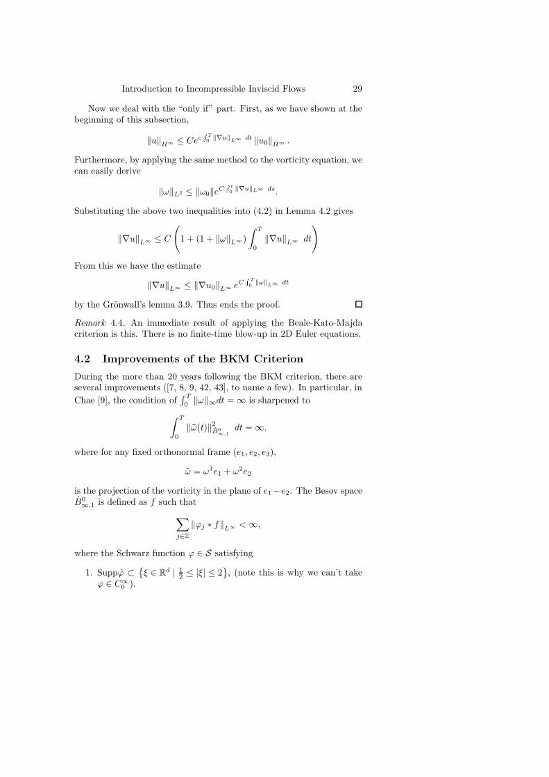
Now we deal with the “only if” part. First, as we have shown at thebeginning of this subsection,
‖u‖Hm ≤ Cec
T0
‖∇u‖L∞ dt ‖u0‖Hm .
Furthermore, by applying the same method to the vorticity equation, wecan easily derive
‖ω‖L2 ≤ ‖ω0‖eC t0‖∇u‖L∞ ds.
Substituting the above two inequalities into (4.2) in Lemma 4.2 gives
‖∇u‖L∞ ≤ C
(1 + (1 + ‖ω‖L∞)
∫ T
0
‖∇u‖L∞ dt
)
From this we have the estimate
‖∇u‖L∞ ≤ ‖∇u0‖L∞ eCT0‖ω‖L∞ dt
by the Gronwall’s lemma 3.9. Thus ends the proof.
Remark 4.4. An immediate result of applying the Beale-Kato-Majdacriterion is this. There is no finite-time blow-up in 2D Euler equations.
4.2 Improvements of the BKM Criterion
During the more than 20 years following the BKM criterion, there areseveral improvements ([7, 8, 9, 42, 43], to name a few). In particular, in
Chae [9], the condition of∫ T
0‖ω‖∞dt = ∞ is sharpened to
∫ T
0
‖ω(t)‖2B0
∞,1dt = ∞.
where for any fixed orthonormal frame (e1, e2, e3),
ω = ω1e1 + ω2e2
is the projection of the vorticity in the plane of e1−e2. The Besov spaceB0
∞,1 is defined as f such that
∑
j∈Z
‖ϕj ∗ f‖L∞ <∞,
where the Schwarz function ϕ ∈ S satisfying
1. Suppϕ ⊂ξ ∈ Rd | 1
2 ≤ |ξ| ≤ 2, (note this is why we can’t take
ϕ ∈ C∞0 ).
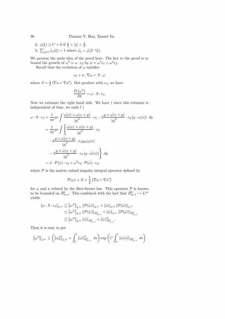
30 Thomas Y. Hou, Xinwei Yu
2. ϕ(ξ) ≥ C > 0 if 23 < |ξ| < 3
2 .
3.∑
j∈Zϕj(ξ) = 1 where ϕj = ϕ(2−jξ).
We present the main idea of the proof here. The key to the proof is tobound the growth of ω3 ≡ ω · e3 by ω = ω1e1 + ω2e2.
Recall that the evolution of ω satisfies
ωt + u · ∇ω = S · ω
where S = 12 (∇u + ∇ut). Dot product with e3, we have
D(ω3)
Dt= ω · S · e3.
Now we estimate the right hand side. We have ( since this estimate isindependent of time, we omit t )
ω · S · e3 =1
4πpv
∫ω(x) × ω(x+ y)
|y|3· e3 − 3
y × ω(x+ y)
|y|5· e3 (y · ω(x)) dy
=1
4πpv
∫ ω(x) × ω(x+ y)
|y|3· e3
−3y × ω(x+ y)
|y|5· e3y3ω3(x)
− 3y × ω(x+ y)
|y|5· e3 (y · ω(x))
dy
= ω · P(ω) · e3 + ω3e3 · P(ω) · e3.
where P is the matrix valued singular integral operator defined by
P(ω) = S =1
2
(∇u+ ∇ut
)
for ω and u related by the Biot-Savart law. This operator P is knownto be bounded on B0
∞,1. This combined with the fact that B0∞,1 → L∞
yields
‖ω · S · e3‖L∞ .∥∥ω3
∥∥L∞ ‖P(ω)‖L∞ + ‖ω‖L∞ ‖P(ω)‖L∞
≤∥∥ω3
∥∥L∞ ‖P(ω)‖B0
∞,1+ ‖ω‖L∞ ‖P(ω)‖B0
∞,1
.∥∥ω3
∥∥L∞ ‖ω‖B0
∞,1+ ‖ω‖2
B0
∞,1.
Then it is easy to get
∥∥ω3∥∥
L∞ ≤(∥∥ω3
0
∥∥L∞ +
∫ t
0
‖ω‖2B0
∞,1ds
)exp
(C
∫ t
0
‖ω(s)‖B0
∞,1ds
)
Introduction to Incompressible Inviscid Flows 31
by integrating the equation for ω3 along one particle trajectory X(α, t),and then applying the Gronwall’s lemma.
Finally, using the Cauchy-Schwarz inequality, and the embeddingB0
∞,1 → L∞ again, we have
∫ T
0
‖ω‖L∞ dt ≤∫ T
0
‖ω‖L∞ dt+
∫ T
0
∥∥ω3∥∥
L∞ dt
≤√TAT +
[∥∥ω30
∥∥L∞ + CA2
T
]T exp
(C√TAT
)
where AT ≡(∫ T
0 ‖ω‖2B2
∞,1dt)1/2
. Thus ends the proof for the necessity
part. The sufficient part is trivial from the embedding Hm → B0∞,1 for
m > 5/2.This result is sharper than the BKM criterion, but its disadvantage
is that it is not as applicable to numerical simulations as the BKM one.For example, it is not always as easy to measure the Besov norm as theL∞ norm accurately in numerical computations.
5 Recent Global Existence Results
In this chapter we review some recent results which are in the same linewith the BKM criterion. Due to the limited scope of this lecture note,we will not be able to cover all relevant results in this area, even forthose results that are related to the Beale-Kato-Majda criterion.
5.1 Sufficient Conditions by Constantin-Fefferman-Majda
In 1996, Constantin-Fefferman-Majda [14] proposed an non-blow-up con-dition based on the BKM criterion. To understand the main idea, we
recall the BKM criterion: If∫ T
0‖ω(·, t)‖L∞ dt <∞, then no blow-up can
happen in [0, T ]. This implies that one should investigate the vorticitymagnitude |ω(x, t)|.
The first step would naturally be deriving the evolution equation forthis quantity. This equation is derived in Constantin [13]. It is
D
Dt|ω| = α(x, t) |ω| . (5.1)
where
α(x, t) ≡ ξ(x, t) · ∇u(x, t) · ξ(x, t)= ξ(x, t) · S(x, t) · ξ(x, t)
32 Thomas Y. Hou, Xinwei Yu
where S(x, t) is the symmetric part of ∇u and ξ(x, t) = ω(x,t)|ω(x,t)| is the
direction of ω(x, t).
Remark 5.1. Note that ξ is well defined only for those points whereω(x, t) 6= 0. For those points where ω(x, t) = 0, ω(x, t) will always be 0as long as the flow is not singular, along the trajectory path of the samepoint, forward and backward in time. This can be seen from the formula
ω(X(α, t), t) = ∇αX · ω(α, 0).
and the fact that ∇αX is non-singular as long as the flow is not singular.So at those points where vorticity vanishes, one can reasonably defineα(x, t) = 0.
(5.1) can be derived by applying the inner product of the vorticityequation (2.8) with ξ, and using the fact that ∂xjξ · ξ = 0 since ξ · ξ = 1.The proof is left as an exercise.
Next we recall that
∇u = pv
∫
R3
∇K(x− y)ω(y) dy + Cω(x).
where C is a third order tensor C = [C1, C2, . . . , Cd] where Cj =∫|z|=1
K(z)zj dz
as defined in the proof to Lemma 4.2. Note that, since Cjω = cj ×ω forsome cj ≡
∫|z|=1
z|z|3
zj dz,
ξ · (Cω) · ξ = 0.
Now it is easy to get
α(x, t) =3
4πpv
∫
R3
(y · ξ(x)) det(y, ξ(x+ y), ξ(x)) |ω(x+ y)| dy|y|3
. (5.2)
where y = y/ |y| is the direction of y, and det(a, b, c) is the determinantof the matrix with columns a, b, c in that order. The constant 3
4π willhave no effect in the following argument, and will thus be neglected fromnow on.
The main idea of Constantin-Fefferman-Majda’s argument comesfrom the following observation. Consider the 2D Euler equations. Weknow that no blow-up can ever occur. Put into the framework of (5.1)and (5.2), we see that the reason can be interpreted as the fact that for2D flows, ξ(x+ y) = ξ(x) = e3 for all x and y, which means α(x, t) ≡ 0.This implies that, if the orientation of the vorticity vectors varies onlymildly, there would be no blow-up. Thus comes the following theorem.First we give some definitions.
Introduction to Incompressible Inviscid Flows 33
Definition 5.2. ( Smoothly directed ). We say a set W0 is smoothlydirected if there exists ρ > 0 and r, 0 < r ≤ ρ
2 such that the followingthree conditions are satisfied.
First, for every q ∈ W ∗0 ≡ q ∈ W0; |ω0(q)| 6= 0 and all time t ∈
[0, T ), the function ξ(·, t) has a Lipschitz extension ( denoted by thesame letter ) to the Euclidean ball of radius 4ρ centered at X(q, t),denoted as B4ρ(X(q, t)), and
M = limt→T
supq∈W∗
0
∫ t
0
‖∇ξ(·, t)‖2L∞(B4ρ(X(q,t))) dt <∞.
Secondly,sup
B3r(Wt)
|ω(x, t)| ≤ m supBr(Wt)
|ω(x, t)|
holds for all t ∈ [0, T ) with m ≥ 0 constant. Here
Wt ≡ X(W0, t).
Thirdly, for all t ∈ [0, T ),
supB4ρ(Wt)
|u(x, t)| ≤ U.
Theorem 5.3. (Constantin-Fefferman-Majda 1996). Assume W0 issmoothly directed. Then there exists τ > 0 and Γ such that
supBr(Wt)
|ω(x, t)| ≤ Γ supBρ(Wt0 )
|ω(x, t0)|
holds for any 0 ≤ t0 < T and 0 ≤ t− t0 ≤ τ .
Noticing that, in (5.2), α(x, t) would also be zero when ξ(x + y) =−ξ(x). This inspires the following pair of definition and theorem.
Definition 5.4. W0 is said to be regularly directed, if there exists ρ > 0such that
supq∈W∗
0
∫ T
0
Kρ(X(q, t)) dt <∞
where
Kρ(x) =
∫
|y|≤ρ
(y · ξ(x)) det(y, ξ(x+ y), ξ(x)) |ω(x+ y)| dy|y|3
.
Theorem 5.5. (Constantin-Fefferman-Majda 1996) Assume W0 regu-larly directed. Then there exists a constant Γ such that
supq∈W0
|ω(X(q, t), t)| ≤ Γ supq∈W0
|ω0(q)|
holds for all t ∈ [0, T ].
34 Thomas Y. Hou, Xinwei Yu
Remark 5.6. An easy corollary to either theorem is that, there will beno blow-up up to time T .
The remaining of this subsection is devoted to the proof of Theorem5.3. As will be seen during the proof, proving Theorem 5.5 is quite easyand will thus be omitted.
We decomposeα(x) = αin(x) + αout(x)
where
αin(x) = pv
∫χ
( |y|ρ
)(y · ξ(x)) det(y, ξ(x+ y), ξ(x)) |ω(x+ y)| dy
|y|3
and
αout(x) =
∫ (1 − χ
( |y|ρ
))(y·ξ(x)) det(y, ξ(x+y), ξ(x)) |ω(x+ y)| dy
|y|3
with χ(r) being a smooth non-negative function satisfying χ(r) = 1for r ≤ 1/2 and 0 for r ≥ 1. Then, recalling ω(x) = ∇ × u(x) andξ(x + y) |ω(x+ y)| = ω(x + y), we can do integration by parts in αout
and get
|αout(x)| . ρ−1
∫
|y|≥ρ/2
|u(x+ y)| dy|y|3
.
Then by Cauchy-Schwarz and the conservation of∫|u|2 dx, we easily
reach|αout(x)| . Cρ−5/2 ‖u0‖L2
which remains bounded.To estimate αin, denote
Gρ(x) = sup|y|≤ρ
|∇ξ(x + y)| .
Observe that det(y, ξ(x+y), ξ(x)) = y·(ξ(x+ y) × ξ(x)) = y·((ξ(x+ y) − ξ(x)) × ξ(x))which is bounded by Gρ(x) |y|. Thus we have
|αin(x)| ≤ Gρ(x)I(x)
with
I(x) ≡∫χ
( |y|ρ
)|ω(x+ y)| dy
|y|2.
Next we split I = I1 + I2, where
I1(x) =
∫χ
( |y|δ
)χ
( |y|ρ
)|ω(x+ y)| dy
|y|2
Introduction to Incompressible Inviscid Flows 35
and
I2(x) =
∫ [1 − χ
( |y|δ
)]χ
( |y|ρ
)|ω(x+ y)| dy
|y|2
with δ ≤ ρ/2. Clearly we get
|I1(x)| ≤ CδΩδ
whereΩδ(x) = sup
|y|≤δ
|ω(x+ y)|
by evaluating the integration through polar coordinates. To estimate I2,we replace |ω(x+ y)| by ξ(x + y) · ω(x+ y) = ξ(x + y) · (∇× u(x+ y))and invoke integration by parts, which gives
I2(x) =
∫u(x+ y) ·
∇×
[ξ(x+ y)
1
|y|2χ
( |y|ρ
)(1 − χ
( |y|δ
))]dy.
By putting ∇× on each of the four terms, we decompose I2 into fourterms as follows:
I2(x) = A+B +D + E.
It is easy to see that
|A| ≤ CGρ(x)
∫
|y|≤ρ
|u(x+ y)| dy|y|2
,
|B| ≤ C
∫|u(x+ y)|
[1 − χ
( |y|δ
)]χ
( |y|ρ
)dy
|y|3,
|D| ≤ C
ρ
∫
|y|≤ρ
|u(x+ y)| dy
|y|2
and
|E| ≤ C
δ
∫
δ2≤|y|≤δ
|u(x+ y)| dy|y|2
.
If we denoteUρ(x) = sup
|y|≤ρ
|u(x+ y)| ,
then we can easily estimate
|A| ≤ CρUρ(x)Gρ(x)
|D| , |E| ≤ CUρ(x)
and|B| ≤ CUρ(x) log
(ρδ
).
36 Thomas Y. Hou, Xinwei Yu
Putting them together, we have
|α(x)| ≤ Aρ(x)[1 + log
(ρδ
)]+Gρ(x)δΩδ(x).
where
Aρ(x) = Cρ−5/2 ‖u0‖L2 + CGρ(x)Uρ(x)(1 + ρGρ(x)).
Studying what we have for a while, we see that if we can replaceΩδ(x) by |ω(x)|, then by taking δ = |ω(x)|−1
, we will have
∫ T
0
|α| dt ≤∫ T
0
Gρ(x)2 dt <∞
by the smoothly directness of our setW0, since we have Uρ to be boundedall the time. And this will effectively end the proof. So the final stepshould be to relate Ωδ(x) with |ω(x)|, although the final proof doesn’tgo along the idea described above for technical reasons.
Consider a bunch of trajectories X(q, t) and a neighborhood
B4ρ ≡ (x, t) : 0 ≤ t < T, ∃q ∈ W0, |X(q, t) − x| ≤ 4ρ .
By the smoothly directness,
sup(x,t)∈B4ρ
|u(x, t)| ≤ U <∞
and
M = limt→T
supq∈W∗
0
∫ t
0
G24ρ (X(q, s)) ds <∞.
Now define
Br(Wt) = x; ∃q ∈W0, |x−X(q, t)| ≤ r
with 2r ≤ ρ.Let
τ =r
4U
be a (possibly very short) time interval. Denote
wr(t) = supBr(Wt)
|ω(x, t)| .
By assumptionw3r(t) ≤ mwr(t).
Now consider x ∈ Br(Wt) for some t < T . The Lagrangian trajectorypassing through x at time t is denoted X(q′, t). Note that q′ may not be
Introduction to Incompressible Inviscid Flows 37
in W0. Nevertheless, if r ≤ ρ2 and 0 ≤ t−s ≤ τ then X(q′, s) ∈ B2r(Ws),
i.e.,|X(q, s) −X(q′, s)| ≤ 2r ≤ ρ
for some q ∈W0. Then it follows that
Gρ(X(q′, s)) ≤ G4ρ(X(q, s))
and
|α(X(q′, s))| ≤ A4ρ(X(q, s))[1 + log
ρ
δ
]+G4ρ(X(q, s))δΩδ(X(q′, s)).
Denoting
A(s) = supq∈W∗
0
A4ρ(X(q, s))
G(s) = supq∈W∗
0
G4ρ(X(q, s)).
Then integrating (5.1) would give us
|ω(X(q′, t))| ≤ Ke
tt0A(s)[1+log(ρ/δ)]+G(s)δΩδ(X(q′,s)) ds
.
whereK = wρ(t0).
Now we choose δ ≤ r, then X(q′, s) ∈ B2r(Ws) and by assumption
Ωδ(X(q′, s)) ≤ mwr(s),
which implies
wr(t) ≤ Ke
tt0
A(s)[1+log(ρ/δ)]+mδG(s)wr(s) ds
for any 0 < δ ≤ r and 0 ≤ t− t0 ≤ τ .To simplify, define
A = A(t, t0) =
∫ t
t0
A(s) ds
and
Q = Kρ
∫ T
0
G(s) ds.
Let
y(t) = maxt0≤s≤t
(wr(s)
K
),
andρ
δ= max
my(t)Q,
ρ
r
.
38 Thomas Y. Hou, Xinwei Yu
Then we obtain
y(t) ≤(ρδ
)A
e1+A.
Finally, we can choose τ such that
A(t, t0) ≤1
2.
This can be done since by assumption A is integrable. Now fix this τ ,we have
y(t) ≤ max
me3Q;
ρ
mrQ
≡ Γ
and thus ends the proof.
5.2 Sufficient Conditions by Deng-Hou-Yu
The result by Constantin, Fefferman and Majda reveals the subtletybetween the smoothness of the vorticity direction field and the accumu-lation rate of vorticity. But on the other hand, their theorems are notquite applicable to various numerical simulations studying the blow-upissue of the 3D Euler equations in recent years. The most interestingones among them are Kerr [26, 27, 28, 29] and Pelz [39, 40]. From theirobservations the following seem to hold for flows that may be singular,i.e., flows that seems to have the critical singular vorticity growth rate(T−t)−1 for some T > 0 (Note: unforced flows that have higher vorticitygrowth rate have never been observed):
1. Large vorticity, or more specifically, those |ω| ≥ c ‖ω‖L∞ , are con-centrated in small regions of length O
((T − t)1/2
)in the vorticity
direction and with cross-section area O((T − t)2
). These regions
look like two vortex sheets with thickness O(T − t) meeting at anangle.
2. The vorticity direction field ξ(x, t) looks more regular inside thisregion than outside, where ξ(x, t) is wildly helical.
Checking these observations against Definition 5.2 and Theorem 5.3 (Note that Definition 5.4 is obviously unverifiable with numerical quan-tities, so we won’t consider Theorem 5.5. ), we see that the conditionsthere are not satisfied. The main reason is that, according to numericalsimulations, the “smoothly directed” region can never have fixed size,instead is always rapidly shrinking in all three directions. Thus thereis a gap between theoretical theorems and numerical observations andleaving Theorem 5.3 unable to explain the numerical results.
In 2005, Deng, Hou and Yu [19] made a first step in filling this gap.The key is to focus on one vortex line and study its local stretching
Introduction to Incompressible Inviscid Flows 39
behaviors. Before introducing the main result, we introduce some nota-tions.
Denote by Ω(t) the maximum vorticity magnitude at time t. Let Lt
be a family of vortex line segments and L(t) be the length of Lt. DenoteUξ(t) ≡ maxx,y∈Lt |(u · ξ) (x, t) − (u · ξ) (y, t)|, Un(t) ≡ maxLt |u · n|where n is the normal of the curve Lt, i.e., ∂
∂sξ = (ξ · ∇) ξ ≡ κn where
κ is the curvature, and M(t) ≡ max(‖∇ · ξ‖L∞(Lt)
, ‖κ‖L∞(Lt)
). We
also define X(a, t1, t2) as follows:
dX(α, t1, t)
dt= u(X(α, t1, t), t); X(α, t1, t1) = α.
It is related to the usual flow map X(q, t) as follows:
X(q, t2) = X(X(q, t1), t1, t2)
for any q, t1, t2.Now the main theorem reads
Theorem 5.7. (Deng-Hou-Yu, 2005) Assume there is a family of vortexline segments Lt and T0 ∈ [0, T ), such that X(Lt1 , t1, t2) ⊇ Lt2 for allT0 < t1 < t2 < T . We also assume that Ω(t) is monotonically increasingand ‖ω(t)‖L∞(Lt)
≥ c0Ω(t) for some c0 > 0 when t is sufficiently closeto T . Furthermore, we assume that
1. [Uξ(t) + Un(t)M(t)L(t)] . (T − t)−α for some α ∈ (0, 1),
2. M(t)L(t) ≤ C0, and
3. L(t) & (T − t)β for some β < 1 − α.
Then there will be no blow-up in the 3D incompressible Euler flow up totime T .
Remark 5.8. Note that the conditions 1–3 are inspired by the numer-ical observations. In Kerr’s computations, the velocity blows up likeO((T − t)−1/2
), which gives alpha = 1/2. On the other hand, M(t) =
(T − t)−1/2. If we take L(t) = (T − t)1/2, then the second conditionis satisfied, but it would just violate the third condition. Thus Kerr’scomputations fall into the critical case of our theorem.
Remark 5.9. In a follow-up paper [21], Deng, Hou and Yu improved theabove result and obtained non-blowup conditions for the critical case β =1− α. The new conditions depend on some fine relations among the as-ymptotic behaviors of the rescaled quantities (T−t)α [Uξ(t) + Un(t)M(t)L(t)],(T − t)α−1L(t) and the bound C0. In [25], Hou and Li repeated Kerr’scomputations using a pseudo-spectral method with resolution up to
40 Thomas Y. Hou, Xinwei Yu
1536× 1024× 3072 up to T = 19, beyond the singularity time Tc = 18.7predicted by Kerr. They found that there is a tremendous dynamic de-pletion of the vortex stretching term. The velocity field is found to bebounded, and the maximum vorticity does not grow faster than doublyexponential in time. The fact that velocity is bounded allows us to ap-ply the non-blowup conditions of [22], which provides further theoreticalevidence of the non-blowup of the Euler equations with Kerr’s initialdata.
We give a simple proof of the non-blowup result of Deng-Hou-Yu.First we investigate the incompressibility condition of vorticity. ∇ ·
ω = 0. It is easy to see that
∂ |ω|∂s
(x, t) = − (∇ · ξ(x, t)) |ω| (x, t).
where s is the arc length of the vortex line containing (x, t), so that∂∂s = ξ · ∇. This implies that for any two points x, y ∈ Lt, as long as
|∫ y
x∇ · ξds| ≤M(t)L(t) ≤ C, we have
e−M(t)L(t) ≤ |ω(y, t)||ω(x, t)| ≤ eM(t)L(t). (5.3)
Next we study the relation between vorticity magnitude and vortexline stretching. Recall that
ω(X(α, t), t) = ∇αX(α, t) · ω0(α).
Multiplying both side by ξ(X(α, t), t) we have
|ω(X(α, t), t)| = ξ(X(α, t), t) · ∇αX(α, t) · ξ(α) |ω0(α)| .Noticing
ξ(X(α, t), t) =∂X
∂salong the vortex line at time t, and similarly
ξ(α) =∂α
∂β
where β is the arc length parameter at time 0. Substituting these rela-tions in, we have
|ω(X(α, t), t)| =∂X(α, t)
∂s· ∇αX(α, t) · ∂α
∂β|ω0(α)|
=∂X
∂s· ∂X∂β
|ω0(α)|
=
(∂X
∂s· ∂X∂s
)∂s
∂β|ω0(α)|
=∂s
∂β|ω0(α)|
Introduction to Incompressible Inviscid Flows 41
since ∂X∂s = ξ is a unit vector. It is easy to generalize the above result to
prove that∂s
∂β(X(α, t1, t), t) =
|ω(X(α, t1, t), t)||ω(α, t1)|
.
Now we have the relations between any two points on Lt, and be-tween vortex line stretching and growth of vorticity magnitude. A thirdingredient is the evolution equation of sβ . It is easy to see that sβ isgoverned by the same equation as |ω| in (5.1).
D
Dtsβ = ξ · ∇u · ξ sβ
= [(ξ · ∇)(u · ξ) − u · (ξ · ∇)ξ] sβ
= (u · ξ)β − κ (u · n) sβ ,
where we have used ξ · ∇ξ = ∂sξ = κn by the Frenet relationship.Integrating it along Lt and in time, we easily get the estimate
l(t2) ≤ l(t1) +
∫ t2
t1
Uξ dτ +
∫ t2
t1
M(τ)Un(τ)l(τ) dτ
where lt is a segment of Lt such that lt2 = X(lt1 , t1, t2), and l(t) is thearclength of lt.
Next we will show how l(t2)/l(t1) is related to the vorticity growth.
e−(M(t)l(t)+M(t1)l(t1)) |ω(X(α′, t1, t), t)||ω(α′, t1)|
≤ l(t)
l(t1)≤ e(M(t)l(t)+M(t1)l(t1)) |ω(X(α′, t1, t), t)|
|ω(α′, t1)|.
(5.4)The proof of (5.4) is not difficult. Let β denote the arc length parameterat time t1. Denote by lt the vortex line segment from 0 to β, and use sas the arc length parameter at time t. Now by the mean value theorem,we have (β is the arclength variable at t1)
l(t)
l(t1)=
∫ β
0 sβ(η) dη
β= sβ(η′) =
|ω(X(α′′, t1, t), t)||ω(α′′, t1)|
,
for some α′′ on the same vortex line. Now the inequality (5.4) followsfrom (5.3).
Now putting the three ingredients together, we get an estimate forthe vorticity magnitude.
Ωl(t2) ≤ eC0Ωl(t1)
[1 +
1
l(t1)
∫ t2
t1
(Uξ(τ) +M(τ)Un(τ)l(τ)) dτ
].
(5.5)where Ωl(t) denotes the maximum vorticity magnitude along lt.
42 Thomas Y. Hou, Xinwei Yu
Now we start the proof of Theorem 5.7 itself. The idea is the follow-ing. Note that the above inequality actually controls the growth rate ofvorticity. So we can expect to prove non-blow-up if l(t1) does not shrinkto zero too fast. If we assume, in the same spirit as those by Constantin-Fefferman-Majda, that l(t) > c > 0 for some fixed c, then effectively wehave
Ω(t2) ≤ eC0Ω(t1)
and obviously no blow-up can happen. Now we illustrate the proof alongthis simple idea.
We prove by contradiction. First, by translating the initial time wecan assume that the assumptions hold in [0, T ). Define
r ≡ (R/c0) + 1
where R ≡ e2C0 . Recall that C0 is the bound of M(t)L(t), and c0 is thelower bound of ΩL(t)/Ω(t), where ΩL(t) ≡ ‖ω(·, t)‖L∞(Lt)
.If there is a finite time blow-up at time T , then we must have
∫ T
0
Ω(t) dt = ∞
and necessarily Ω(t) ∞ as t T . Take t1, t2, . . . , tn, . . . such that
Ω(tk+1) = rΩ(tk).
Since Ω(t) is monotone by assumption, and T is the smallest time that∫ T
0 Ω(t) dt = ∞, we have tn T as n→ ∞.Now we choose lt2 = Lt2 . By assumptions on Lt, we have lt1 ⊂ Lt1
such that X(lt1 , t1, t2) = lt2 . And furthermore, by using (5.4), we obtain
l(t1) ≥ l(t2)1
R
ΩL(t1)
ΩL(t2)≥ l(t2)
c0R2
1
r& (T − t2)
β ,
where the hidden constant in & is independent of time. Now pluggingthis into (5.5) we have, after some algebra,
Ω(t2) ≤ (r − 1)Ω(t1) +C
(1 − α)c0
Ω(t1)
(T − t2)β(T − t1)
1−α.
Recalling Ω(t2) = rΩ(t1), we have
r ≤ (r − 1) + C(T − t1)
1−α
(T − t2)β
which gives(T − t2) ≤ C(T − t1)
1+2δ
Introduction to Incompressible Inviscid Flows 43
with
δ ≡ 1 − α
β− 1
which is positive by assumption. By taking t1 close enough to T , we cancancel C and have
(T − t2) ≤ (T − t1)1+δ.
Next do the same thing for all pairs (tn, tn+1), ( note that (T−tn)δ <(T − t1)
δ ≤ C−1) we have
(T − tk+1) ≤ (T − tk)1+δ ≤ (T − t1)(1+δ)k ≤ (T − t1)(T − t1)
δk (5.6)
if we take T − t1 < 1.Now we study
∫ T
0 Ω(t) dt = ∞. By assumption that Ω(t) is monotone,we have
Ω(t1)
∞∑
k=1
rk(tk+1 − tk) =
∞∑
k=1
Ω(tk+1)(tk+1 − tk) ≥∫ T
t1
Ω(t) dt = ∞
which implies
(r − 1)
∞∑
l=0
rl(T − tl+1) =
∞∑
l=0
(rl+1 − rl)(T − tl+1)
=
∞∑
l=0
∞∑
k=l+1
(rl+1 − rl)(tk+1 − tk)
=
∞∑
k=1
k−1∑
l=0
(rl+1 − rl)(tk+1 − tk)
=
∞∑
k=1
(rk − 1)(tk+1 − tk)
= ∞.
All the equalities are legitimate since all the terms in the summationsare positive ( Fubini’s theorem ).
On the other hand, from (5.6), we obtain
∞ =
∞∑
k=0
rk(T − tk+1) ≤ (T − t1)
∞∑
k=0
[r(T − t1)
δ]k<∞,
if we choose t1 close to T so that r(T − t1)δ < 1. Therefore, we reach a
contradiction. Thus, we obtain∫ T
t1
Ω(t)dt <∞.
By the BKM criterion, we conclude that there is no finite time blow-upup to T .
44 Thomas Y. Hou, Xinwei Yu
6 Lower Dimensional Models for the 3D Eulerequations
6.1 1-D Model
In 1985, P. Constantin, P. Lax and A. Majda proposed the following 1-Dmodel of the 3D Euler equations.
ωt = Hω · ωwhere H is the Hilbert transform:
Hf = pv
∫
R
f(y)
x− ydy.
The relation to the 3D Euler equations is the following. In 3D Eulerequation, the evolution of the vorticity magnitude is governed by thefollowing equation:
D
Dt|ω| = T (ω) |ω| .
where T is a Calderon-Zygmund operator with a convolution kernel thatis homogeneous of degree −d where d is the dimension. In 1-D, only onesuch singular integral kernel exists, i.e., the Hilbert transform.
This simplified model can be explicitly solved. To solve it, we firstget familiar with some properties of the Hilbert transform.
Lemma 6.1. The Hilbert transform has the following properties:
1. H is bounded from Hm to Hm for all m ≥ 0.
2. H (Hf) = −f .3. H (fg) = f (Hg) + g (Hf) +H (Hf ·Hg).
Proof. Properties (1) and (2) follow immediately from the fact that
Hf(ξ) = sgn(ξ)f(ξ).
For property (3), we check
H(fg) − H(Hf ·Hg) =
∫ ∞
−∞
sgn(ξ)f(η)g(ξ − η) dη
−∫ ∞
−∞
sgn(ξ)sgn(η)sgn(ξ − η)f(η)g(ξ − η) dη
=
∫ ∞
−∞
sgn(ξ) (1 − sgn(η)sgn(ξ − η)) f(η)g(ξ − η) dη
=
∫ ∞
−∞
(sgn(ξ − η) + sgn(η)) f(η)g(ξ − η) dη
= f(Hg) + g(Hf),
Introduction to Incompressible Inviscid Flows 45
and thus ends the proof.
Now we set out to find the explicit solutions. We define
z(x, t) = Hω(x, t) + iω(x, t).
By Lemma 6.1, the equation for z is
dz
dt=
1
2z2
whose explicit solution is
z(t) =2z0
2 − z0t
which implies
ω(x, t) =4ω0(x)
(2 − tHω0)2 + t2ω2
0(x).
It is obvious that ω(x, t) will blow-up at points with ω0(x) = 0 butHω0 > 0.
6.2 The 2-D QG Equation
The 2D QG equation ( see Pedlosky [41] ) is given by
Dθ
Dt≡ θt + u · ∇θ = 0, (6.1)
where θ(x, t) is a scalar, and u is defined by
(−4)1/2
ψ = −θu = ∇⊥ψ
Here (−4)1/2 is defined by
(−4)1/2
ψ =
∫e2πix·ξ2π |ξ| ψ(ξ) dξ
if
ψ =
∫e2πix·ξψ(ξ) dξ.
The 2D QG equation ( aka surface-quasi-geostrophic equations, SQG) describes the variation of the density variation θ at the surface of theearth. The name θ, usually represents temperature, is chosen becausein the case the ideal gas, the density variation is proportional to thetemperature.
To get an explicit form of the formula for ψ in the space variable xinstead of the Fourier modes ξ, we use the following lemma:
46 Thomas Y. Hou, Xinwei Yu
Lemma 6.2. Denote
ha(x) =Γ(a/2)
π(a/2)|x|−a
,
then we have
ha = hN−a
for 0 < <(a) < N , where N is the dimension of the space. Γ is theGamma function, defined as
Γ(s) =
∫ ∞
0
e−tts−1 dt.
Proof. See e.g. Thomas Wolff [46].
By the above lemma we easily derive
ψ(x) = −∫
R2
θ(x + y)
|y| dy.
Thus we get
u(x) =
∫
R2
y⊥
|y|2θ(x+ y) dy.
If we define “vorticity”
ω(x) = ∇⊥θ
we obtain by differentiating (6.1) that
Dω
Dt= ∇u · ω,
from which we can derive
D |ω|Dt
=1
2ξ(∇u+ ∇uT
)ξ |ω|
≡ S(x, t) |ω|
=
∫
R2
(y · ξ⊥(x)
) (ξ(x+ y) · ξ⊥(x)
)
|y|2|ω(x+ y)| dy |ω|
=
∫
R2
(y · ξ(x)) det (ξ(x+ y), ξ(x))
|y|2|ω(x+ y)| dy |ω|
where
ξ(x, t) ≡ ω(x, t)
|ω(x, t)|
Introduction to Incompressible Inviscid Flows 47
as long as it is well-defined, and y = y/ |y|. Note that those points withω(x, t) = 0 is transported by the flow, since ω = 0 implies ∇θ = 0 and
∇θ(X(q, t)) = ∇xθ0(q)
= (∇qX)−1 · ∇qθ0(q).
which means ∇qθ0(q) = 0 ⇔ ∇xθ(X(q, t)) = 0. So those points where ξis not well-defined are not important to the stretching.
Recall that for the evolution of the vorticity magnitude in 3D Euler,we have
D |ω|Dt
= α(x, t) |ω|
where
α(x, t) =3
4π
∫
R3
(y · ξ(x)) det (y, ξ(x+ y), ξ(x))
|y|3|ω(x+ y)| dy.
We see that S(x, t) and α(x, t) indeed share very similar cancellationproperties. Thus the 2D QG equation can be viewed as a 2D model ofthe 3D Euler equation, especially in the vorticity form.
There are several other similarities between 2D QG and 3D Euler.For example, the levelsets of θ(x, t), which are lines that are alwaystangent to ω(x, t) so can be defined as “vortex lines”, are carried by theflow, similar to the vortex lines in the 3D Euler dynamics. For morecomparison between 2D QG and 3D Euler equations, as well as otherproperties of the 2D QG equations, see Constantin-Majda-Tabak [15],or the book by Majda-Bertozzi [35].
Remark 6.3. Note that in the 2D QG equation, we no longer have theproperty
1
2
(∇u−∇uT
)ω = 0
as in the 3D Euler case. This implies that, the “vorticity” here doesn’tsatisfy
Dω
Dt=
1
2
(∇u+ ∇uT
)ω
as in the Euler case. Only the evolution of the vorticity magnitude |ω|satisfies the same equation as in the 3D Euler equation.
6.2.1 Existence and blow-up Criteria
By the same technique as in Chapter 2, we can prove the local in timeexistence and blow-up criterion.
48 Thomas Y. Hou, Xinwei Yu
Theorem 6.4. ( Constantin-Majda-Tabak [15] ). If the initial valueθ0(x) belongs to the Sobolev space Hk(R2) for some integer k ≥ 3, thenthere is a smooth solution θ(x, t) ∈ Hk(R2) for the 2D QG equation foreach time t, in a sufficiently small time interval [0, T ∗), where T ∗ ischaracterized by
‖θ(·, t)‖k ∞ as t T ∗
and can be estimated from below by
T ∗ &1
1 − ‖θ0‖k
.
We can also apply the technique for the BKM criterion in Chapter 4to obtain similar blow-up criteria:
Theorem 6.5. ( Constantin-Majda-Tabak [15] ). Consider the uniquesmooth solution of the 2D QG equations with initial data θ0(x) ∈ Hk(R2)for some k ≥ 3. Then the following are equivalent:
1. The time interval [0, T ∗) for some T ∗ < ∞ is maximal for thesolution to be in Hk(R2).
2. The vorticity magnitude accumulates so rapidly that
∫ T
0
‖ω(·, t)‖L∞ dt ∞ as T ∞
3. Let S∗(t) ≡ maxx∈R2 S(x, t), then
∫ T∗
0
S∗(t) dt = ∞.
There are, though, properties that seems to hold only in the 2D QGcase. For example, when we assume that there is a smooth curve x(t),such that each point (x(t), t) is an isolated maximum of |ω(x, t)|, we canhave the following result:
d
dt‖ω(·, t)‖L∞ = S(x(t), t) ‖ω(·, t)‖L∞ .
To prove it, let q(t) be the Lagrange marker of the points (x(t), t), i.e.,
X(q(t), t) = x(t)
Introduction to Incompressible Inviscid Flows 49
then we have
d
dt‖ω(·, t)‖L∞ =
d
dt|ω(x(t), t)|
=d
dt|ω (X(q(t), t), t)|
=D
Dt|ω| (x(t), t) + ∇x |ω| · ∇qX · q
= S(x(t), t) |ω(x(t), t)|= S(x(t), t) ‖ω(·, t)‖L∞
Note that ∇x |ω| = 0 by our assumption that x(t) is an isolated maxi-mum.
The above result implies that, under the assumption on x(t), wecan just consider S(x, t) for the particular point (x(t), t) instead of themaximum of S(x, t) over the whole space. The assumption on x(t) is verylikely to hold in practical cases according to various numerical results,see e.g. Constantin-Majda-Tabak [15].
Remark 6.6. It is claimed in Constantin-Majda-Tabak [15] that the as-sumption on x(t) can be dropped with a more lengthy proof, while thatproof is omitted.
6.2.2 Global existence result by Constantin-Majda-Tabak
In their 1994 paper [15], Constantin, Majda and Tabak studied the evo-lution of the vorticity magnitude both numerically and theoretically,concluded that when the vorticity direction ξ(x, t) varies not too fastin space, there can be no finite time blow-up, i.e., the classical solutionexists globally in time.
To understand the basic idea, we recall the evolution equation for|ω|:
D |ω|Dt
= S(x, t) |ω|
where
S(x, t) =
∫
R2
(y · ξ⊥(x)
) (ξ(x + y) · ξ⊥(x)
)
|y|2|ω(x+ y)| dy.
In general, since S(x, t) = Tω with T being a singular integral oper-ator, ‖S(·, t)‖L∞ can not be bounded by ‖ω(·, t)‖L∞ . Even if it can, theright hand side would be quadratic and give us a finite time blow-up.But if we make assumptions on ξ(x+y), the situation would be different.We illustrate this through several examples.
50 Thomas Y. Hou, Xinwei Yu
Example 6.7. ( Constantin-Majda-Tabak [15] ). We consider the clas-sical frontogenesis with trivial topology. Let
x2 = f(x1)
be a smooth curve in the plane, we study the possibility that the solutionθ(x, t) developing a sharp front along this curve, through the simplifiedansatz
θ(x, t) = F
(x2 − f(x1)
δ(t)
),
where F (s) is a smooth function on R, with the properties that F (s) = 1for s ≥ 3, F (s) = 0 for s ≤ 1 and F ′(s) ≥ 0 for all s. Assume that
δ(t) → 0, as t→ T ∗
for some T ∗ <∞.We can plug the formula for θ into the 2D QG equation and get
F ′
[d
dt
(1
δ(t)
)+ u ·
(f ′(x1)
1
)(1
δ(t)
)]= 0.
Since obviously ‖ω‖L∞ (t) ∼ 1/δ(t), we have the estimate
d
dt(log ‖ω‖L∞ (t)) . ‖u‖L∞ (t).
It can be shown that for 2D QG equation
‖u‖L∞ (t) . log ‖ω‖L∞ . (6.2)
We see that the growth rate of the maximum vorticity is at most doubleexponential, and there will be no finite time blow-up.
The last thing is to prove the estimate (6.2), which first appears inCordoba [17].
Recall that, for teh 2D QG equation, we have
u = (−4)−1/2 ω =
∫1
|y|ω(x+ y) dy.
Now let r > 0 fixed, large enough, ρ ∈ (0, r) to be specified later, and χbe the standard cut-off function, we decompose u into 3 terms as follows
|u(x)| = Uin(x) + Umed(x) + Uout(x)
where
Uin(x) =
∫χ
( |x|ρ
)1
|y|ω(x+ y) dy
≤ ‖ω‖L∞ ρ
Introduction to Incompressible Inviscid Flows 51
by simply using polar coordinates. For Umed, we have
Umed(x) =
∫χ
( |x|r
)(1 − χ
( |x|ρ
))1
|y|ω(x+ y) dy
=
∫χ
( |x|r
)(1 − χ
( |x|ρ
))1
|y|∇⊥θ(x+ y) dy
.
∫
2r≥|y|≥ρ/2
1
|y|2θ(x + y) dy +
1
ρ
∫
2ρ≥|y|≥ρ/2
θ(x+ y)
|y| dy
+1
r
∫
2r≥|y|≥r/2
1
|y|θ(x + y) dy
. −‖θ‖L∞ (1 + | log ρ|) = −‖θ0‖L∞ (1 + | log ρ|),
as long as ρ < c < 1 for some fixed constant c. Here we have used the
fact that ∇χ(
|x|ρ
)= 0 for all |x| ≤ ρ/2 or |x| ≥ 2ρ and the maximum
of |θ| is bounded by the initial data.Now we estimate Uout,
Uout(x) =
∫ (1 − χ
( |x|r
))1
|y|∇⊥θ(x + y) dy
.1
r
∫
2r≥|y|≥r/2
1
|y|θ(x + y) dy +
∫
|y|≥r/2
θ(x+ y)dy
|y|2≡ I + II.
I is obviously bounded by some constant since ‖θ‖∞ ≤ ‖θ0‖∞. For II,we use he Cauchy-Schwarz inequality and the fact that the L2 norm ofθ is conserved. We get
II . r−1 ‖θ0‖L2
which is also bounded by a constant.Finally, if ‖ω‖L∞ ≤ e, (6.2) trivially holds. If not, taking ρ = ‖ω‖−1
L∞
immediately gives the desired estimate.
We look at another example, the singular thermal ridge.
Example 6.8. (Constantin-Majda-Tabak [15] ). The assumptions aresimilar to the previous example, the only difference is that F (s) = 0 forboth s ≥ 3 and s ≤ 1, with F ′(s) > 0 for 1 < s < 2, F ′(s) < 0 for2 < s < 3. There can be no finite time blow-up for these ridges either.The proof is similar to that in the last example and is omitted.
The above two examples implies that, for θ whose levelsets form sim-ple geometries, there may be no finite time blow-up. To quantify whatwe mean by “simple geometry”, we use the direction of the “vorticityvectors” ξ = ω/ |ω|. The precise statement of the theorem is the follow-ing (Constantin-Majda-Tabak [15]):
52 Thomas Y. Hou, Xinwei Yu
Definition 6.9. A set Ω0 is smoothly directed if there exists ρ > 0 suchthat
supq∈Ω0
∫ T
0
|u (X(q, t), t)|2 dt <∞
and
supq∈Ω∗
0
∫ T
0
‖∇ξ(·, t)‖L∞(Bρ(X(q,t),t))) dt <∞
where Bρ(x) is the ball of radius ρ centered at x and
Ω∗0 = q ∈ Ω0 | |ω0(q)| 6= 0 .
We use the following notation:
Ωt = X(Ω0, t)
OT (Ω0) = (x, t) | x ∈ Ωt, 0 ≤ t ≤ T Theorem 6.10. Assume Ω0 is smoothly directly, then
supOT (Ω0)
|∇θ(x, t)| <∞
i.e., there can be no blow-up in OT (Ω0).
Definition 6.11. We say that the set Ω0 is regularly directed if thereexists ρ > 0 such that
supq∈Ω∗
0
∫ T
0
Kρ (X(q, t)) dt <∞
where
Kρ(x) =
∫
|y|≤ρ
∣∣y · ξ⊥(x)∣∣ ∣∣ξ(x + y) · ξ⊥(x)
∣∣ |ω(x+ y)| dy
|y|2
Theorem 6.12. Assume that Ω0 is regularly directed, then
supOT (Ω0)
|ω(x, t)| <∞
The proofs to these theorems are similar to the ones in the globalexistence results by Constantin-Fefferman-Majda for the 3D Euler equa-tions, only less technical. The main difference is that here we have aconserved quantity θ, whose Lp norm is conserved for all 1 ≤ p ≤ ∞.This simplifies the proof a lot. First, S(x, t) is bounded by
|S(x, t)| ≤ C[G(t) |u(x, t)| + (ρG(t) + 1)
(G(t) ‖θ‖L∞ + ρ−2 ‖θ‖L2
)]
where G(t) ≡ sup|y|≤ρ |∇ξ(x + y)| for some fixed ρ > 0, via similarestimates as in Chapter 2. Next we integrate the above in time and usethe Cauchy-Schwarz inequality. For details see Constantin-Majda-Tabak[15].
Introduction to Incompressible Inviscid Flows 53
Remark 6.13. The reader may notice that our condition on the maximumvelocity, i.e., L2-integrable in time, is much weaker than the one in the3D Euler case, i.e., L∞ bounded. This is because, in 2D QG, we haveω = (∂2,−∂1)θ with θ being bounded. For 3D Euler, we have ω = ∇×uand we do not have a priori bound on u. Thus in the case of the 3DEuler equation, we have a term
G(t)2U(t)
which won’t be integrable if U(t) ≡ ‖u‖L∞ (t) is not bounded in addition.
6.2.3 Global existence result by Cordoba and Fefferman
The results by Constantin-Majda-Tabak claims that, as long as the di-rection field of the levelsets are smooth enough locally around the maxi-mum stretching point, there can be no finite time blow-up in the 2D QGequations. This leaves one candidate for finite-time blow-up in their nu-merical simulations, i.e., the “hyperbolic saddle” situation. In fact, theyperformed detailed numerical experiments and found that the maximumvorticity can be fitted by 1/ (8.25 − t)
1.7, which suggests a finite time
blow-up. In 1997, Ohkitani and Yamada re-did the simulations andpushed further to higher resolutions ( [38] ), and found that the sameresult can be fitted as well by double exponential growth, indicating thatno finite time blow-up can occur, at least up to the time of their compu-tations. Subsequently, Constantin-Nie-Schorghofer [16] ) found that thedouble exponential is in several aspects a better fit, suggesting that nofinite-time blow-up can occur. Around the same time, D. Cordoba [17]proved that under some mild assumptions, the hyperbolic saddles willnot cause a finite time blow-up, instead the growth of |ω| is bounded byquadruple exponential. The proof is technical and we will not reproduceit here.
In 2002, D. Cordoba and C. Fefferman [18] considered a case thatcovers most of the scenarios considered by Constantin-Majda-Tabak andthe hyperbolic saddle case by Cordoba, which they called “semi-uniformcollapse”, and obtained the numerically observed double exponentialgrowth by clever estimates. We will recap their work here.
Assume that there is an interval [a, b] such that
θ(x1, φρ(x1, t), t) = G(ρ)
for x1 ∈ [a, b], where x2 = φρ(x1, t) is a level curve of θ, φρ ∈ C1 ([a, b] × [0, T ))for some alleged blow-up time T . By a “semi-uniform” collapse we meanthat the level sets are almost parallel to each other (Note that the sharp-ening front and ridge in Examples 6.7 and 6.8 satisfy that the level curvesare exactly parallel to each other). More specifically, if we denote
δ(x1, t) ≡ |φρ(x1, t) − φρ′(x1, t)| ,
54 Thomas Y. Hou, Xinwei Yu
then δ satisfiesmin[a,b]
δ(x1, t) ≥ cmax[a,b]
δ(x1, t).
By this assumption, we always have
|ω(x1, φρ(x1, t), t)| ∼1
δ(x′1, t)
for any x1, x′1 ∈ [a, b].
From this observation, it is enough to consider
I =d
dt
(∫ b
a
[φρ2(x1, t) − φρ1
(x1, t)] dx1
)
since the quantity being differentiated is comparable to |ω|−1( Note that,
since different level curves will never cross, the sign of the difference isfixed. ).
We computed
dtφρ(x1, t)
for some fixed ρ. First note that, the curve (x1, φρ(x1, t)) is transportedby the flow, since it always parametrized the level curve θ = G(ρ). Sowe have
d
dtφρ(x1, t) = u2 − u1
∂φρ
∂x1=
d
dx1ψ(x1, φρ(x1, t), t)
where ψ = (−4)−1/2
θ so that u = ∇⊥ψ. The first equality can beseen by drawing a picture and studying the difference between φρ at tand t + δt, or go through the argument using the QG equation as inCordoba-Fefferman [18].
Now it is immediate that
I = ψ(b, φρ2(b, t), t) − ψ(a, φρ2
(a, t), t)
+ψ(a, φρ1(a, t), t) − ψ(b, φρ2
(b, t), t).
Let
A(t) ≡ 1
b− a
∫ b
a
[φρ2(x1, t) − φρ1
(x1, t)] dx1,
we have∣∣∣∣d
dtA(t)
∣∣∣∣ . sup[a,b]
|ψ(x1, φρ2(x1, t), t) − ψ(x1, φρ1
(x1, t), t)| .
Finally we prove a general estimate
|ψ(z1, t) − ψ(z2, t)| . ||z1 − z2| log |z1 − z2|| .
Introduction to Incompressible Inviscid Flows 55
Obviously, that will end the proof, and bound the maximum growth bysome double exponential.
Recall that
ψ(x, t) = (−4)−1/2 θ = −∫θ(x + y)
|y| dy.
Taking τ = |z1 − z2| we have
ψ(z1) − ψ(z2) =
∫θ(y)
(1
|y − z1|− 1
|y − z2|
)dy
=
∫
|y−z1|≤2τ
+
∫
2τ<|y−z1|≤k
+
∫
k<|y−z1|
= I1 + I2 + I3
where k > 2τ is some constant.Now trivially,
|I1| ≤ Cτ.
For I2, by the mean value theorem∣∣∣∣
1
|y − z1|− 1
|y − z2|
∣∣∣∣ = τ
∣∣∣∣∇1
|y − z′|
∣∣∣∣
for some z′ lying on the line segment connecting z1 and z2. Thus we canfurther bound it by
τ maxs
1
|y − s|2
where the maximum is taken over the line connecting z1 and z2. Now itis clear that
|II| ≤ Cτ |log τ | .III is also trivially bounded by Cτ using the conservation of the L2
norm of θ, and the mean value theorem.Thus ends the proof.
6.2.4 Final Remarks about the QG equation
The global existence/blow-up issue for the 2D quasi-geostrophic equa-tion is still open today, and solving it would for sure shed light on andhelp solving the same problem for the 3D Euler equations. A recentprogress is Deng-Hou-Li-Yu [22], where the authors applied the methoddeveloped in their papers dealing with the 3D Euler equations [19, 21],and obtained triple exponential growth bound for ‖∇θ‖∞ under verymild conditions. Furthermore, under slightly stronger conditions the au-thors show that the growth rate of ‖∇θ‖∞ can be bounded by double
56 Thomas Y. Hou, Xinwei Yu
exponential, which is the real growth rate observed in numerical com-putations. High resolution numerical computations carried out by theauthors suggest that these conditions are indeed satisfied in the 2D QGflow. This observation suggests that these conditions may have touchedthe essence of the QG dynamics. The authors are currently making aneffort to further investigate this problem.
7 Vortex Patch
A vortex patch is a bounded, simply connected, open material domainDt such that the vorticity is constant inside it and 0 elsewhere. It is aspecial case of the L1 ∩ L∞ weak solutions. Here we will describe theproblem without using the general weak solution formalism.
7.1 The contour dynamics equation (CDE)
By definition and our expectation that the vorticity will be conservedalong particle trajectories ( should check that they really exist ), it is(hopefully) enough to derive an equation that governs the evolution ofthe boundary.
Assume that the solution do behave this way, i.e., the vorticity atany time t is ω0 in some smooth region D(t) and 0 outside, where D(t)is smoothly parametrized by t. Then the velocity is
u(x, t) =ω0
2π
∫
D(t)
(x− y)⊥
|x− y|2dy.
By the Divergence Theorem we can rewrite it as a contour integral
u(x, t) =ω0
2π
∫
∂D(t)
log |x− y| n⊥(y)dS(y),
where n(y) is the unit outer normal vector. Note that in our setting,D(t) and then ω(x, t) is determined by the evolution of the boundary∂D(t). If we parametrize it by x = x(s, t), we have
∂x(s, t)
∂t= −ω0
2π
∫
∂D(t)
log |x(s, t) − x(s′, t)| ∂x∂s′
(s′, t) ds′
This is called the CDE ( contour dynamics equation ). It can be checkedthat as long as the boundary remains smooth enough, ω(x, t) defined bythe CDE is a weak solution.
In [34], A. Majda observed that, Y = ∂x∂s satisfies an evolution equa-
tion very similar to the 1-D model:
DY
Dt= (M(Y ))Y,
Introduction to Incompressible Inviscid Flows 57
where M(Y ) is a matrix whose entries are Cauchy integrals on a curve,i.e., a generalization of the 1D Hilbert transform. He further conjecturedthat a finite time singularity would form from smooth initial data.
In 1991, J.-Y. Chemin [10] proved that in fact the above resemblanceis just superficial. The evolution of the vortex patch boundary behavesmuch better than the 3D Euler equations. Namely, the boundary willremain in C1,µ if it is started in this function class. In [4], A. Bertozziand P. Constantin give an alternative proof that is easier to understand.We will present this proof in the next subsection.
7.2 Levelset formulation and global existence
Let 0 < µ < 1 and D be a simply connected, bounded and open subsetof the plane whose boundary is C1,µ smooth, i.e., for any x0 ∈ ∂D thereexists a ball B(x0; r0) and a C1,µ function ϕ : R 7→ R such that, after arotation,
∂D ∩B(x0, r0) =x ∈ B(x0, r0) | x2 = ϕ(x1)
.
Now we introduce the levelset formulation. Let ϕ ∈ C1,µ(R2) be suchthat
D = x | ϕ(x) > 0and |∇ϕ| ≥ c > 0 on the boundary. By the implicit function theoremwe see that ∂D defined by ϕ = 0 is indeed C1,µ. Thus to establish thelong time existence, we only need to show the existence of C1,µ functionϕ(x, t) such that D(t) = x | ϕ(x, t) > 0 and ∇ϕ(x, t) is bounded belowby c > 0 uniformly in t.
It is easy to see that the evolution of ϕ(x, t) should be governed by
ϕt + u · ∇ϕ = 0 (7.1)
and thusD
Dt∇⊥ϕ ≡ ∇u · ∇⊥ϕ
which looks similar to the 3D Euler equation.We need to show two things, first
∥∥∇⊥ϕ∥∥
C0,µ is bounded above,
second∣∣∇⊥ϕ
∣∣ = |∇ϕ| is bounded below at ϕ = 0.
Proposition 7.1. Let u be the velocity field associated to a vortex patch.Denote
σ(z) =
2z1z2
|z|2z2
2−z2
1
|z|2
z2
2−z2
1
|z|2− 2z1z2
|z|2
.
Then
∇u(x) =ω0
2πpv
∫
D
σ(x − y)
|x− y|2dy +
ω0
2
(0 −11 0
)χD(x).
58 Thomas Y. Hou, Xinwei Yu
Proof. The proof is straightforward, similar to those in Chapter 4.
First we need to notice some properties of σ(x − y).
1. It is smooth outside of the origin and homogeneous of degree 0.
2. It is symmetric with respect to reflection about the origin, i.e.,σ(z) = σ(−z).
3. It has mean 0 on the unit circle.
4. By (2) and (3), it has mean 0 on any half circle centered at 0.
By (1) the kernel in the integral is a singular integral kernel. But oneimportant difference with the 3D Euler or other model equations ( 1DConstantin-Lax-Majda Model, 2D QG ) is that, this singular integralkernel is acting on a characteristic function instead of ∇⊥ϕ, thus it canbe expected to behave much better than the 3D Euler equation.
To see this point, we consider a naıve approach. Instead of the tech-nical C1,γ , suppose we would like to prove that the level set equation(7.1) is well-posed in C1. For this purpose, it is enough to prove that‖∇u‖L∞ is bounded. We have
∇u(x) =ω0
2πpv
∫
D
σ(x − y)
|x− y|2dy +
ω0
2
(0 −11 0
)χD(x).
So it is enough to prove that
pv
∫
D
σ(x − y)
|x− y|2dy
remains bounded for all x. Suppose that we only need to worry aboutthe integral
I(x) ≡ pv
∫
D∩B(x,δ)
σ(x− y)
|x− y|2dy
for some δ > 0. Obviously when d(x) ≡ dist(x, ∂D) ≥ δ, I(x) = 0. Onthe other hand, when d(x) < δ, we need subtle cancellations. To getsome insight, assume that locally ∂D is x2 = 0, and x = (0, x2) ∈ Dwith δ > x2 > 0. By the properties of σ, we see that σ has mean 0 onsemi-circles. This implies that,
I(x) =
∫
Deff
σ(x − y)
|x− y|2dy,
where Deff ≡ D ∩ (B(x, δ) \B(x, d(x)) ∩ 0 < y2 < d(x) is illustrated inthe following figure by the shaded area:
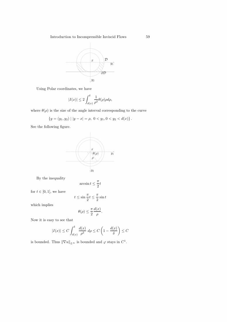
Introduction to Incompressible Inviscid Flows 59
x
∂Dy2
y1
D
Using Polar coordinates, we have
|I(x)| ≤ 2
∫ δ
d(x)
1
ρ2θ(ρ)ρdρ,
where θ(ρ) is the size of the angle interval corresponding to the curve
y = (y1, y2) | |y − x| = ρ, 0 < y1, 0 < y2 < d(x) .
See the following figure.
ρ
y2
y1
x
θ(ρ)
By the inequality
arcsin t ≤ π
2t
for t ∈ [0, 1], we have
t ≤ sinπ
2t ≤ π
2sin t
which implies
θ(ρ) ≤ π
2
d(x)
ρ.
Now it is easy to see that
|I(x)| ≤ C
∫ δ
d(x)
d(x)
ρ2dρ ≤ C
(1 − d(x)
δ
)≤ C
is bounded. Thus ‖∇u‖L∞ is bounded and ϕ stays in C1.
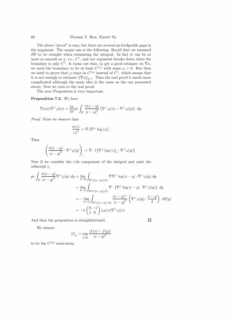
60 Thomas Y. Hou, Xinwei Yu
The above “proof” is easy, but there are several un-bridgeable gaps inthe argument. The major one is the following. Recall that we assumed∂D to be straight when estimating the integral. In fact it can be atmost as smooth as ϕ, i.e., C1, and our argument breaks down when theboundary is only C1. It turns out that, to get a good estimate on ∇u,we need the boundary to be at least C1,µ with some µ > 0. But thenwe need to prove that ϕ stays in C1,µ instead of C1, which means thatit is not enough to estimate ‖∇u‖L∞ . Thus the real proof is much morecomplicated although the main idea is the same as the one presentedabove. Now we turn to the real proof.
The next Proposition is very important.
Proposition 7.2. We have
∇u(x)∇⊥ϕ(x) =ω0
2πpv
∫
D
σ(x− y)
|x− y|2(∇⊥ϕ(x) −∇⊥ϕ(y)
)dy.
Proof. First we observe that
σ(z)
|z|2= ∇
(∇⊥ log |z|
).
Thus(σ(x − y)
|x− y|2· ∇⊥ϕ(y)
)
i
= ∇ ·((∇⊥ log |z|
)i· ∇⊥ϕ(y)
).
Now if we consider the i-th component of the integral and omit thesubscript i,
pv
∫
D
σ(x − y)
|x− y|2∇⊥ϕ(y) dy = lim
δ→0
∫
D∩|x−y|≥δ
∇∇⊥ log |x− y| · ∇⊥ϕ(y) dy
= limδ→0
∫
D∩|x−y|≥δ
∇ ·(∇⊥ log |x− y| · ∇⊥ϕ(y)
)dy
= − limδ→0
∫
D∩|x−y|=δ
(x− y)⊥
|x− y|2(∇⊥ϕ(y) · x− y
δ
)dS(y)
= −π(
0 −11 0
)χD(x)∇⊥ϕ(x).
And then the proposition is straightforward.
We denote
|f |µ = supx 6=y
|f(x) − f(y)||x− y|µ
to be the C0,µ semi-norm.
Introduction to Incompressible Inviscid Flows 61
Proposition 7.3. There exists a constant C = C(µ) such that
∣∣∇u(·)∇⊥ϕ(·)∣∣µ≤ C (1 + ‖∇u‖L∞) |∇ϕ|µ .
Proof. Let x, h ∈ R2. We estimate
2π
ω0
∣∣(∇u · ∇⊥ϕ)(x+ h) −
(∇u · ∇⊥ϕ
)(x)∣∣
≤∣∣∣∣∣pv∫
D
σ(x+ h− y)
|x+ h− y|2(∇⊥ϕ(x+ h) −∇⊥ϕ(y)
)dy
∣∣∣∣∣
+
∣∣∣∣∣pv∫
D
σ(x − y)
|x− y|2(∇⊥ϕ(x) −∇⊥ϕ(y)
)dy
∣∣∣∣∣
≤∣∣∣∣∣pv∫
D∩|x−y|≤2|h|
σ(x+ h− y)
|x+ h− y|2(∇⊥ϕ(x + h) −∇⊥ϕ(y)
)dy
∣∣∣∣∣
+
∣∣∣∣∣
∫
D∩|x−y|>2|h|
σ(x + h− y)
|x+ h− y|2(∇⊥ϕ(x + y) −∇⊥ϕ(y)
)dy
∣∣∣∣∣
+
∣∣∣∣∣pv∫
D∩|x−y|≤2|h|
σ(x − y)
|x− y|2(∇⊥ϕ(x) −∇⊥ϕ(y)
)dy
∣∣∣∣∣
+
∣∣∣∣∣
∫
D∩|x−y|>2|h|
(σ(x− y)
|x− y|2− σ(x+ h− y)
|x+ h− y|2
)(∇⊥ϕ(x+ h) −∇⊥ϕ(y)
)dy
∣∣∣∣∣≡ I1 + I2 + I3 + I4.
We estimate them one by one.For I1, we use the fact that ϕ ∈ C1,µ and get
I1 ≤ C |h|µ |∇ϕ|µ .
For I2, by Cotlar’s lemma, we have
I2 ≤ C (‖∇u‖∞ + 1)
For I3, Similar to I1, we have
I3 ≤ C |h|µ |∇ϕ|µ .
Lastly, for I4, by the mean value theorem, we have
I4 ≤∫
D∩|x−y|≥2|h|
|h| C
|x− y|3|x− y|µ |∇ϕ|µ ≤ C |h|µ |∇ϕ|µ .
62 Thomas Y. Hou, Xinwei Yu
Remark 7.4. Cotlar’s lemma is the following result:
For any singular integral kernel K(x), define
Kε(x) ≡
0 |x| ≤ εK(x) |x| > ε
.
Then there is a constant C > 0, such that for any ε > 0,
|Kε ∗ f | (x) ≤ C (M(K ∗ f)(x) +M(f)(x)) .
where M(f) denotes the maximal function of f .
M(f) ≡ supr>0
1
|B(x, r)|
∫
B(x,r)
f(y) dy.
Thus in particular, if both K ∗ f and f are in L∞, then we can re-place M(K ∗ f)(x) by ‖K ∗ f‖L∞ and M(f) by ‖f‖L∞ . For more aboutCotlar’s lemma, see e.g. Section 1.7 of Stein [45] or Chapter 7 of Meyer-Coifman [37].
Our next task is to give a upper bound for ‖∇u‖L∞ . Denote theinfimum norm of a function f on ∂D by
|f |inf = infx∈∂D
|∇ϕ(x)| .
Proposition 7.5. Let u be the velocity and ϕ be a solution to (7.1).Then there is a constant C = C(µ) > 0 such that
‖∇u‖L∞ ≤ C |ω0|(
1 + log
(|∇ϕ|µ|∇ϕ|inf
)).
Proof. First note that we only need to estimate the principal integral
pv
∫
D
σ(x− y)
|x− y|2dy.
Denote
δ =|∇ϕ|inf
|∇ϕ|µ.
and d(x) = dist(x, ∂D) for any x ∈ R2. Intuitively, the main difficultywould come from near the boundary.
Introduction to Incompressible Inviscid Flows 63
First we assume d(x) ≥ δ. Take η small enough, we have∣∣∣∣∣
∫
D∩|x−y|≥η
σ(x − y)
|x− y|2dy
∣∣∣∣∣ ≤∣∣∣∣∣
∫
D∩η≤|x−y|≤d(x)
σ(x − y)
|x− y|2dy
∣∣∣∣∣
+
∣∣∣∣∣
∫
D∩|x−y|>d(x)
σ(x − y)
|x− y|2dy
∣∣∣∣∣
=
∣∣∣∣∣
∫
D∩|x−y|>d(x)
σ(x− y)
|x− y|2dy
∣∣∣∣∣
≤∣∣∣∣∣
∫
D∩|x−y|>d(x)
1
|x− y|2dy
∣∣∣∣∣
≤∣∣∣∣∣
∫
d(x)<|x−y|≤R
1
|x− y|2dy
∣∣∣∣∣
where πR2 is the area of D, which is conserved by the imcompressibilityof the flow. The last inequality can be readily checked by using Polarcoordinates and the fact that 1
r2 is monotonically decreasing in r. Theproof is left as an exercise. Now it is easy to see that the integral isbounded by what we want.
Now for the case d(x) < δ. Again taking η small enough, we have∣∣∣∣∣
∫
D∩|x−y|≥η
σ(x − y)
|x− y|2dy
∣∣∣∣∣ ≤∣∣∣∣∣
∫
D∩η≤|x−y|≤d(x)
σ(x− y)
|x− y|2dy
∣∣∣∣∣
+
∣∣∣∣∣
∫
D∩d(x)≤|x−y|<δ
σ(x − y)
|x− y|2dy
∣∣∣∣∣
+
∣∣∣∣∣
∫
D∩|x−y|≥δ
σ(x − y)
|x− y|2dy
∣∣∣∣∣ .
We know that the first integral vanishes due to symmetry, and the thirdterm can be estimated as in the d(x) ≤ δ case.
For the second one, we denote
S = d(x) ≤ |x− y| ≤ δ
and study its special geometrical properties. The heuristic is the follow-ing. Assume that the boundary is a straight line, then we try to boundthe integral by estimating the area of the integration in which the inte-gral doesn’t vanish. This is where the regularity of the boundary comesin to play. To make the above idea rigorous, we denote by x the point on∂D such that d(x, x) = d(x). Let L be the line through x in the direc-tion that is tangent to ∂D at x. Then the annulus d(x) ≤ |x− y| ≤ δ
64 Thomas Y. Hou, Xinwei Yu
is divided into two half annuli. Denote the one containing x by As andthe other by Al. First note that the integration on Al vanishes. So
∣∣∣∣∣
∫
S∩D
σ(x− y)
|x− y|2dy
∣∣∣∣∣ =
∣∣∣∣∣
∫
(As∩D)∪(Al∩Dc)
σ(x− y)
|x− y|2dy
∣∣∣∣∣
≤∫
(As∩D)∪(Al∩Dc)
C
|x− y|2dy.
Note that S should more and more resembles a half-annulus as d(x) → 0.So our integral should vanish. We estimate the area of Se ≡ (As ∩D) ∪(Al ∩ Dc). Write it in polar coordinates and denote by H(Eρ) the 1-DHausdorff measure of
θ ∈ (0, 2π] | (ρ, θ) ∈ Se .for d(x) ≤ ρ ≤ δ. By the Geometric lemma that will be proved later,
H(Eρ) ≤ C
(d(x)
ρ+(ρδ
)µ)
and then the result is straightforward.
Now we prove the Geometric Lemma.
Lemma 7.6. (Geometric Lemma). We have
H(Eρ) ≤ 2π
[(1 + 2µ)
d(x0)
ρ+ 2µ
(ρδ
)µ]
for all ρ ≥ d(x0), 1 > µ > 0 and x0 so that d(x0) < δ =(|∇φ|inf / |∇ϕ|µ
)1/µ
.
Proof. Let
Sρ(x0) = z | |z| = 1, x = x0 + ρz ∈ D ,Σ(x0) = z | |z| = 1,∇xϕ(x) · z ≥ 0
where x ∈ ∂D such that |x0 − x| = d(x0). This point exists since theboundary is C1,µ. Then we have
Eρ = [Sρ\Σρ] ∪ [Σρ\Sρ] .
The readers should draw a picture to see what Eρ looks like (there aretwo cases, x0 ∈ D and x0 6∈ D). Note that since ϕ(x) > 0 for x ∈ D, thedirection of ∇ϕ at x should be pointing inward instead of outward.
We use polar coordinates and denote the angle for a point z in Eρ
by θ(z), with θ(z) defined by
sin θ(z) =∇ϕ(x) · z
|∇ϕ(x)| · |z| .
See the following illustration.
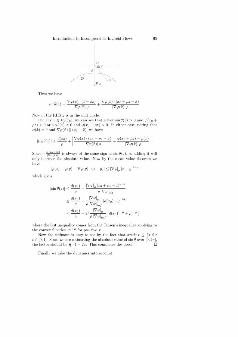
Introduction to Incompressible Inviscid Flows 65
x0
θ(z)
D
x
∇ϕz
Thus we have
sin θ(z) =∇ϕ(x) · (x− x0)
|∇ϕ(x)| ρ +∇ϕ(x) · (x0 + ρz − x)
|∇ϕ(x)| ρ .
Now in the RHS z is in the unit circle.For any z ∈ Eρ(x0), we can see that either sin θ(z) > 0 and ϕ(x0 +
ρz) < 0 or sin θ(z) < 0 and ϕ(x0 + ρz) > 0. In either case, noting thatϕ(x) = 0 and ∇ϕ(x) ‖ (x0 − x), we have
|sin θ(z)| ≤ d(x0)
ρ+
∣∣∣∣∇ϕ(x) · (x0 + ρz − x)
|∇ϕ(x)| ρ − ϕ(x0 + ρz)− ϕ(x)
|∇ϕ(x)| ρ
∣∣∣∣ .
Since −ϕ(x0+ρz)|∇ϕ(x)|ρ is always of the same sign as sin θ(z), so adding it will
only increase the absolute value. Now by the mean value theorem wehave
|ϕ(x) − ϕ(y) −∇ϕ(y) · (x− y)| ≤ |∇ϕ|µ |x− y|1+µ
which gives
|sin θ(z)| ≤ d(x0)
ρ+
|∇ϕ|µ |x0 + ρz − x|1+µ
ρ |∇ϕ|inf
≤ d(x0)
ρ+
|∇ϕ|µρ |∇ϕ|inf
[d(x0) + ρ]1+µ
≤ d(x0)
ρ+ 2γ
|∇ϕ|µρ |∇ϕ|inf
[d(x0)
1+µ + ρ1+µ]
where the last inequality comes from the Jensen’s inequality applying tothe convex function x1+µ for positive x.
Now the estimate is easy to see by the fact that arcsin t ≤ π2 t for
t ∈ [0, 1]. Since we are estimating the absolute value of sin θ over [0, 2π],the factor should be π
2 · 4 = 2π. This completes the proof.
Finally we take the dynamics into account.
66 Thomas Y. Hou, Xinwei Yu
Proposition 7.7. If the initial data ϕ0 ∈ C1,µ(R2), such that D0 =ϕ0(x) > 0 is simply connected and bounded. And |∇ϕ0| ≥ C > 0 onthe boundary ∂D0, then the following a priori estimates holds:
1. ‖∇ϕ(·, t)‖L∞ ≤ ‖∇ϕ0‖L∞ exp(∫ t
0 ‖∇u(·, s)‖L∞ ds);
2. |∇ϕ(·, t)|inf ≥ |∇ϕ0|inf exp(−∫ t
0‖∇u(·, s)‖L∞ ds
);
3. |∇ϕ(·, t)|µ ≤ |∇ϕ0|µ exp((C0 + µ)
∫ t
0 ‖∇u(·, s)‖L∞ ds).
Proof. Let X = X(α, t) denote a particle trajectory and
Y (α, t) = ∇⊥ϕ(X(α, t), t).
Then we haved
dtY (α, t) = ∇u(X(α, t), t)Y (α, t).
and therefore ∣∣∣∣d
dtlog |Y (α, t)|
∣∣∣∣ ≤ ‖Du(·, t)‖L∞ .
Now by Gronwall’s lemma we have
e−
t0‖∇u‖L∞ ds ≤ |Y (α, t)|
|∇⊥ϕ0(α)| ≤ e
t0‖∇u‖L∞ ds,
which proves both (1). and (2).For (3), we write the integral formulation of the equation for ∇⊥ϕ,
∇⊥ϕ(x, t) = ∇⊥ϕ0(X(x,−t)) +
∫ t
0
(∇u∇⊥ϕ
)(X(x, s− t), s) ds.
And we estimate
∣∣∇⊥ϕ(x + h, t) −∇⊥ϕ(x, t)∣∣ ≤
∣∣∇⊥ϕ0 (X(x+ h,−t)) −∇⊥ϕ0 (X(x,−t))∣∣
+
∣∣∣∣∫ t
0
((∇u∇⊥ϕ
)(X(x+ h, s− t), s) −
(∇u∇⊥ϕ
)(X(x, s− t), s)
)ds
∣∣∣∣≤∣∣∇⊥ϕ0
∣∣µ‖∇X(·,−t)‖µ
L∞ |h|µ
+
∫ t
0
∣∣∇u∇⊥ϕ(·, s)∣∣µ‖∇X(·, s− t)‖µ
L∞ |h|µ ds.
For the evolution of ∇X , we have
d
dt∇X(z,−t) = −∇u (X(z,−t),−t)∇X(z,−t).
Introduction to Incompressible Inviscid Flows 67
Now by the Gronwall’s lemma we have
‖∇X(·, s− t)‖L∞ ≤ exp
(∫ t
s
‖∇u(·, s′)‖L∞ ds′).
Plug it into the inequality above, we get the estimate in (3).
Finally we put everything together, and obtain the following theorem:
Theorem 7.8. Given ω0 6= 0, D0 a simply connected, bounded, C1,µ
smooth domain with 0 < µ < 1, and a function ϕ0 ∈ C1,µ(R2) suchthat D0 = ϕ0 > 0, |∇ϕ0|inf ≥ C > 0, then the solution ϕ belongs
to C1,µfor all time. Furthermore, there exists a constant C > 0, whichdepends only on the initial data such that
1. ‖∇u(·, t)‖L∞ ≤ ‖∇u0‖L∞ eCt,
2. |∇ϕ(·, t)|µ ≤ |∇ϕ0|µ exp((C0 + µ) eCt
),
3. ‖∇ϕ(·, t)‖L∞ ≤ ‖∇ϕ0‖L∞ exp(eCt),
4. |∇ϕ(·, t)|inf ≥ |∇ϕ0|inf exp(−eCt
).
Proof. We have
log |∇ϕ|inf ≥ log |∇ϕ0|inf − C
∫ t
0
(1 + log
|∇ϕ|µ|∇ϕ|inf
)ds
after taking logarithm on both sides of estimate (2) in Proposition 5.2.7.Similarly we obtain
log |∇ϕ|µ ≤ log |∇ϕ0|µ + (C0 + µ)
∫ t
0
(1 + log
|∇ϕ|µ|∇ϕ|inf
)ds.
Combining these two, we have
log|∇ϕ|µ|∇ϕ|inf
≤ log|∇ϕ0|µ|∇ϕ0|inf
+ (C0 + µ+ 1)
∫ t
0
(1 + log
|∇ϕ|µ|∇ϕ|inf
)ds.
By Gronwall’s lemma, we easily get
log|∇ϕ|µ|∇ϕ|inf
≤ CeCt.
This also provides a bound for ∇u in (1) from Proposition 5.2.5. Theothers are straightfoward by using the estimate on ∇u given by Property(1).
Remark 7.9. The problem of global existence of vortex patch with bound-ary only C1 or worse is still open. In [6], J. Carrillo and J. Soler showednumerically that, for initial boundary that is only Lipschitz continuous,the evolution develops cusps from corners.
68 Thomas Y. Hou, Xinwei Yu
References
[1] Adams, R. A., Sobolev Spaces, Academic Press, New York 1975.
[2] Arnold V. I., Khesin, B., Topological Methods in Hydrodynamics,Applied Mathematical Sciences 125, Springer, 1998.
[3] Bergh J., Lofstrom, J., Interpolation Spaces: An Introduction,Springer-Verlag, 1976.
[4] Bertozzi, A., Constantin, P., Global regularity for vortex patches,Comm. Math. Phys., 152 (1993), 19–26.
[5] Caflisch, R. E., Orellana, O. F., Long Time Existence for a SlightlyPerturbed Vortex Sheet, Comm. Pure Appl. Math., 39 (1986), 807–838.
[6] Carrillo, J. A., Soler, J., On the Evolution of an Angle in a VortexPatch, Journal of Nonlinear Science, 10 (2000), no. 1, 23–47.
[7] Chae, D., On the well-posedness of the Euler equations in theTriebel-Lizorkin spaces, Comm. Pure Appl. Math., 55 (2002), 654-678.
[8] Chae, D., On the Euler equations in the critical Triebel-Lizorkinspaces, Arch. Ration. Mech. Anal., 170 (2003), 185-210.
[9] Chae, D., Remarks on the blow-up criterion of the three-dimensionalEuler equations, Nonlinearity, 18 (2005), 1021-1029.
[10] Chemin, J. Y., Sur le mouvement des particules d’un fluide parfaitincompressible bidimensionnels, Invent. Math., 103 (1991), 599–629.
[11] Chorin, A., Vorticity and Turbulence, Applied Mathematical Sci-ences 103, Springer-Verlag, 1994.
[12] Chorin, A. J., Marsden, J. E., A Mathematical Introduction to FluidMechanics, 2nd ed., Texts in Applied Mathematics 4, Springer-Verlag, 1990.
[13] Constantin, P., Geometric statistics in turbulence, SIAM Review,36 (1994), 73–98.
[14] Constantin, P., Fefferman, C., and Majda, A., Geometric con-straints on potentially singular solutions for the 3-D Euler equa-tions, Comm. PDE, 21 (1996), no. 3&4, 559–571.
[15] Constantin, P., Majda, A. J., Tabak, E., Formation of strong frontsin the 2-D quasigeostrophic thermal active scalar, Nonlinearity7(1994), 1495–1533.
[16] Constantin, P., Nie, Q., Schorghofer, N., Nonsingular Surface-Quasi-Geostrophic Flow, Phys. Lett. A, 241(1998), 168–172.
Introduction to Incompressible Inviscid Flows 69
[17] Cordoba, D., Nonexistence of simple hyperbolic blow-up for thequasi-geostrophic equation, Annals of Mathematics, 148 (1998),1135–1152.
[18] Cordoba, D., Fefferman, C., Growth of solutions for QG and 2DEuler equations, J. AMS, 15 (2002), no. 3, 665–670.
[19] Deng, J., Hou, T. Y., and Yu, X., Geometric Properties and Non-blowup of 3-D Incompressible Euler Flow, Comm. PDE., 30 (2005),no. 1, 225-243.
[20] Deng, J., Hou, T. Y., and Yu, X., A Level Formulation for the3D Incompressible Euler Equations, Methods and Applications ofAnalysis, 12 (2005), no. 4, 427-440.
[21] Deng, J., Hou, T. Y., and Yu, X., Improved Geometric Conditionsfor Non-blowup of the 3D Incompressible Euler Equation, Comm.PDE., 31 (2006), no. 2, 293-306.
[22] Deng, J., Hou, T. Y., Li, R. and Yu, X., Level Set Dynamics andNon-blowup of the 2D Quasi-geostrophic Equation, accepted byMethods and Applications of Analysis, 2008.
[23] Ebin, D.G., Fischer, A. E., and Marsden, J. E., Diffeomorphismgroups, hydrodynamics and relativity. In Vanstone, J., editor, Prod.of the 13th Biennial Seminar of Canadian Mathematical Congress,135 – 279, Montreal.
[24] Goodman, J., Hou, T.Y., Lowengrub, J., The Convergence of thePoint Vortex Method for the 2-D Euler Equations, Comm. PureAppl. Math., 43 (1990), 415-430.
[25] Hou, T. Y., Li, R., Dynamic Depletion of Vortex Stretcing and Non-Blowup of the 3-D Incompressible Euler Equations, J. NonlinearScience, 16 (2006), no. 6, 639-664.
[26] Kerr, R. M., Evidence for a singularity of the three-dimensionalincompressible Euler equations, Phys. Fluids A, 5 (1993), 1725–1746.
[27] Kerr, R. M., The role of singularities in Euler, in Small-scale struc-ture in hydro and magnetohydrodynamic turbulence, eds. Pouquet,A., Sulem, P. L., Lecture Notes, Springer-Verlag, 1995.
[28] Kerr, R. M., Euler Singularities and Turbulence, in 19th ICTAMKyoto’ 96, Eds. Tatsumi, T., Watanabe, E., Kambe, T., ElsevierScience, 1997.
[29] Kerr, R. M., The Outer Regions in Singular Euler, in Funda-mental Problematic Issues in Turbulence, eds. Tsinober and Gyr,Birkhauser, 1998.
70 Thomas Y. Hou, Xinwei Yu
[30] Kozono, H., Taniuchi, Y., Bilinear estimates in BMO and to theNavier-Stokes equations, Math. Z., 235 (2000), 173–194.
[31] Lamb, H., Hydrodynamics, 6th ed., Dover, 1945.
[32] Lions, P. L., Mathematical Topics in Fluid Mechanics, Vol. 1. In-compressible Models, Oxford Lecture Series in Mathematics and itsApplications 3, Oxford Science Publications, 1996.
[33] Lopes Filho, M.C., Nussenzveig Lopes, H.J. and Zheng, Y., Weaksolutions to the equations of incompressible, ideal flow. Text of mini-course for the 22nd Brazilian Colloquium of Mathematics, 1999. Fulltext at http://www.ime.unicamp.br/˜mlopes/publications.html.
[34] Majda, A., Vorticity and the mathematical theory of Incompressiblefluid flow, Comm. Pure. Appl. Math., 39 (1986), 187–220.
[35] Majda, A. J., Bertozzi, A. L., Vorticity and Incompressible Flow,Cambridge Texts in Applied Mathematics, Cambridge UniversityPress, 2002.
[36] Marchioro, C., Pulvirenti, M., Mathematical Theory of Incompress-ible Nonviscous Fluids, Chapter 6. Applied Mathematical Sciences96. Springer-Verlag, 1994.
[37] Meyer, Y., Coifman, R., Wavelets: Calderon-Zygmund operatorsand multilinear operators, Cambridge University Press, 1997.
[38] Ohkitani, K., Yamada, M., Inviscid and inviscid-limit behavior of asurface quasigeostrophic flow, Phys. Fluids 9 (1997), no. 4, 876–882.
[39] Pelz, R. B., Locally self-similar, finite-time collapse in a high-symmetry vortex filament model, Physical Review E, 55 (1997),no. 2, 1617–1620.
[40] Pelz, R. B., Symmetry and the hydrodynamic blow-up problem, J.Fluid Mech., 444 (2001), 299–320.
[41] Pedlosky, J., Geophysical Fluid Dynamics, 345 – 368, 653–670,Springer, 1987.
[42] Planchon, F., An extension of the Beale-Kato-Majda criterion forthe Euler equations, Comm. Math. Phys., 232 (2003), 319-326.
[43] Ponce, G., Remarks on a paper by J. T. Beale, T. Kato, and A.Majda, Comm. Math. Phys., 98 (1985), 349–353.
[44] Stein, E., Singular Integrals and Differentiability Properties of Func-tions, Princeton University Press, 1970.
[45] Stein, E., Harmonic Analysis, Princeton University Press, 1993.
[46] Wolff, T., Lecture Notes on Harmonic Analysis, University LectureSeries, 29, AMS, 2003.
Acta Numerica (2009), pp. 1–70 c© Cambridge University Press, 2009
doi: 10.1017/S0962492906420018 Printed in the United Kingdom
Blow-up or no blow-up? A unifiedcomputational and analytic approach to
3D incompressible Euler andNavier–Stokes equations
Thomas Y. HouApplied and Computational Mathematics, 217-50,
Caltech, Pasadena, CA 91125, USAE-mail: [email protected]
Whether the 3D incompressible Euler and Navier–Stokes equations can de-velop a finite-time singularity from smooth initial data with finite energyhas been one of the most long-standing open questions. We review some re-cent theoretical and computational studies which show that there is a subtledynamic depletion of nonlinear vortex stretching due to local geometric regu-larity of vortex filaments. We also investigate the dynamic stability of the 3DNavier–Stokes equations and the stabilizing effect of convection. A uniquefeature of our approach is the interplay between computation and analysis.Guided by our local non-blow-up theory, we have performed large-scale com-putations of the 3D Euler equations using a novel pseudo-spectral methodon some of the most promising blow-up candidates. Our results show thatthere is tremendous dynamic depletion of vortex stretching. Moreover, weobserve that the support of maximum vorticity becomes severely flattenedas the maximum vorticity increases and the direction of the vortex filamentsnear the support of maximum vorticity is very regular. Our numerical ob-servations in turn provide valuable insight, which leads to further theoreticalbreakthrough. Finally, we present a new class of solutions for the 3D Eulerand Navier–Stokes equations, which exhibit very interesting dynamic growthproperties. By exploiting the special nonlinear structure of the equations, weprove nonlinear stability and the global regularity of this class of solutions.
2 T. Y. Hou
CONTENTS
1 Introduction 22 Dynamic depletion of vortex stretching in 3D
Euler equations 63 Dynamic stability of 3D Navier–Stokes equations 294 Stabilizing effect of convection for 3D
Navier–Stokes 445 Concluding remarks 65References 67
1. Introduction
The question of whether the 3D incompressible Navier–Stokes equationscan develop a finite-time singularity from smooth initial data is one of themost long-standing open problems in fluid dynamics and mathematics. Thisis also one of the seven Millennium Open Problems posted by the ClayMathematical Institute (see www.claymath.org). The understanding of thisproblem could improve our understanding on the onset of turbulence andthe intermittency properties of turbulent flows.
The 3D incompressible Navier–Stokes equations are given by
ut + (u · ∇)u = −∇p+ ν∆u, (1.1)∇ · u = 0, (1.2)
with initial condition u(x, 0) = u0(x). Here u is velocity, p is pressure, andν is viscosity. We consider only the initial value problem and assume thatthe solution decays rapidly at infinity. Defining vorticity by ω = ∇ × u,then ω is governed by
ωt + (u · ∇)ω = ∇u · ω + ν∆ω. (1.3)
The first term on the right-hand side of (1.3) is called the vortex stretchingterm, which is absent in the two-dimensional problem. Note that ∇u isformally of the same order as ω. Thus the vortex stretching term has aformal quadratic scaling with respect to vorticity. This formal quadraticnonlinearity in the vortex stretching term is the main difficulty in study-ing the dynamic stability and global regularity of the 3D Navier–Stokesequations. Under suitable smallness assumptions on the initial condition,global existence and regularity results have been obtained for some time(Ladyzhenskaya 1970, Constantin and Foias 1988, Temam 2001, Majda andBertozzi 2002). But these methods based on energy estimates do not gen-eralize to the 3D Navier–Stokes with large data. Energy estimates seem tobe too crude to give a definite answer to whether diffusion is strong enoughto control the nonlinear growth due to vortex stretching. A more refined
Blow-up or no blow-up? 3
analysis seems to be needed, which takes into account the special nature ofthe nonlinearities and their local interactions.
We believe that the global regularity of the 3D Navier–Stokes equations isclosely related to that of the 3D Euler equations. Since the nonlinearity ofthe 3D Navier–Stokes equations is supercritical, the balance among differentnonlinear terms in the Euler equations may play an even more important rolethan the diffusion term. Thus, it makes sense to investigate the mechanismwhich may lead to finite-time blow-up or dynamic depletion of the nonlinearvortex stretching in the 3D Euler equations.
There has been some interesting development in the theoretical under-standing of the 3D incompressible Euler equations. In particular, Con-stantin, Fefferman and Majda have shown that the local geometric regular-ity of vortex lines can play an important role in depleting nonlinear vortexstretching (Constantin 1994, Constantin, Fefferman and Majda 1996). In-spired by their work, Deng, Hou and Yu (2005, 2006a) recently showed thatgeometric regularity of vortex lines, even in an extremely localized regioncontaining the maximum vorticity, can lead to depletion of nonlinear vortexstretching, thus avoiding finite-time singularity formation of the 3D Eulerequations. To obtain these results, Deng, Hou and Yu used a Lagrangianapproach and explored the connection between the stretching of local vor-tex lines and the growth of vorticity. In particular, they showed that if thevortex lines near the region of maximum vorticity satisfy some local geo-metric regularity conditions and the maximum velocity field is integrable intime, then no finite-time blow-up is possible. These localized non-blow-upcriteria provide stronger constraints on the local geometry of a potentialfinite-time singularity.
There have been many computational attempts to find finite-time sin-gularities of the 3D Euler and Navier–Stokes equations: see, e.g., Chorin(1982), Pumir and Siggia (1990), Kerr and Hussain (1989), Grauer andSideris (1991), Shelley, Meiron and Orszag (1993), Kerr (1993), Caflisch(1993), Boratav and Pelz (1994), Fernandez, Zabusky and Gryanik (1995),Pelz (1997), Grauer, Marliani and Germaschewski (1998), Kerr (2005). Oneexample that has been studied extensively is the interaction of two per-turbed antiparallel vortex tubes. This example is interesting because ofthe vortex reconnection observed for the corresponding Navier–Stokes equa-tions. It is natural to ask whether the 3D Euler equations would develop afinite-time singularity in the limit of vanishing viscosity. Kerr (1993, 2005)presented numerical evidence which suggested a finite-time singularity ofthe 3D Euler equations for two perturbed antiparallel vortex tubes. Kerr’sblow-up scenario is consistent with the non-blow-up criterion of Beale, Katoand Majda (1984) and that of Constantin, Fefferman and Majda (1996).But it falls into the critical case of Deng, Hou and Yu’s local non-blow-upcriteria (Deng, Hou and Yu 2005, 2006a).
4 T. Y. Hou
Guided by this local geometric non-blow-up analysis, Hou and Li (2006)performed extremely large-scale computations with resolution up to 1536 ×1024× 3072 to re-examine Kerr’s blow-up scenario (Kerr 1993). They useda novel pseudo-spectral method with a 36th-order Fourier smoothing func-tion which keeps a significant portion of the Fourier modes beyond the 2/3cut-off point in the Fourier spectrum for the 2/3 de-aliasing rule. Theirextensive numerical results demonstrated that the pseudo-spectral methodwith the high-order Fourier smoothing gives a much better performancethan the pseudo-spectral method with the 2/3 de-aliasing rule. In par-ticular, they showed that the Fourier smoothing method captures about12 ∼ 15% more effective Fourier modes than the 2/3 de-aliasing methodin each dimension. For 3D Euler equations, the total number of effectivemodes in the Fourier smoothing method is about 20% more than that in the2/3 de-aliasing method. This is a very significant increase in the resolutionfor a large-scale computation.
There were several interesting findings in the large-scale computations ofHou and Li (2006) for the 3D Euler equations using the initial data for theantiparallel vortex tubes. First, they discovered a surprising dynamic can-cellation in the vortex stretching term due to the local geometric regularityof the vortex filaments. Vortex stretching was found to deplete dynamicallyfrom a formally quadratic nonlinearity to a much weaker O(ω log(ω)) typeof nonlinearity, which leads to only double exponential growth in the maxi-mum vorticity. Secondly, they showed that the velocity field is bounded upto T = 19, beyond the alleged singularity time T = 18.7 of Kerr (2005).With a bounded velocity field, the non-blow-up criterion of Deng, Hou andYu (2005) applies, which provides theoretical support for their computa-tional results. Thirdly, they found that the vorticity vector near the pointof maximum vorticity aligns almost perfectly with the second eigenvector ofthe rate of strain tensor. The second eigenvalue of the rate of strain tensoris the smallest eigenvalue and does not seem to grow dynamically, while thefirst and third eigenvalues grow very rapidly in time. This is further strongevidence for the dynamic depletion of vortex stretching.
Inspired by the numerical findings of their paper of 2006, Hou and Li(2008a) investigated the dynamic stability of the 3D Navier–Stokes equa-tions by introducing an exact 1D model of the axisymmetric Navier–Stokesequations along the symmetry axis. This 1D model is exact in the sensethat one can construct a family of exact solutions for the 3D Navier–Stokesequations from this 1D model. Thus the 1D model preserves some es-sential features of the 3D Navier–Stokes equations. What is surprising isthat they obtained a Lyapunov function which satisfies a new maximumprinciple. This provides a pointwise estimate on the dynamic stability ofthe Navier–Stokes equations. The traditional energy estimates are inca-pable of capturing such subtle cancellation effects. Based on the global
Blow-up or no blow-up? 5
regularity of the 1D model, they constructed a new class of solutions forthe 3D Euler and Navier–Stokes equations, which exhibit very interestingdynamic growth properties, but remain smooth for all times.
Motivated by the work of Hou and Li (2008a), Hou and Lei (2009b) furtherproposed a new 3D model to study the stabilizing effect of convection. Thismodel was derived by neglecting the convection term from a reformulatedaxisymmetric Navier–Stokes equations. It shares almost all the propertiesof the 3D Navier–Stokes equations. In particular, the strong solution ofthe model satisfies an energy identity similar to that of the full 3D Navier–Stokes equations. They proved a non-blow-up criterion of Beale–Kato–Majda type as well as a non-blow-up criterion of Prodi–Serrin type for themodel. Moreover, they proved that, for any suitable weak solution of the 3Dmodel in an open set in space-time, the one-dimensional Hausdorff measureof the associated singular set is zero (Hou and Lei 2009a). This partialregularity result is an analogue of the Caffarelli–Kohn–Nirenberg theory(Caffarelli, Kohn and Nirenberg 1982) for the 3D Navier–Stokes equations.
Despite the striking similarity at the theoretical level between the 3Dmodel and the Navier–Stokes equations, the former has a completely differ-ent behaviour from the full Navier–Stokes equations. Hou and Lei’s studyshowed that the 3D model seems to form a finite-time singularity, whilethe mechanism of generating such a finite-time singularity is removed whenconvection is added back to the 3D model. Convection seems to play a veryimportant role in stabilizing the potential blow-up of the Navier–Stokesequations. This result may have an important impact on future global reg-ularity analysis of 3D Navier–Stokes equations. Up to now, most analysisuses energy estimates in which convection plays no role at all. Such globalmethods of analysis are too crude. Their studies suggest that one needs todevelop a new localized analysis which can in essence exploit the stabilizingeffect of convection.
There has been some interesting development in the study of the 3D in-compressible Navier–Stokes equations and related models. By exploiting thespecial structure of the governing equations, Cao and Titi (2007) provedthe global well-posedness of the 3D viscous primitive equation for large-scale ocean and atmospheric dynamics. For the axisymmetric Navier–Stokesequations, Chen, Strain, Tsai and Yau (2008, 2009) and Koch, Nadirashvili,Seregin and Sverak (2009) recently proved that if |u(x, t)| ≤ C∗|t|−1/2, whereC∗ is allowed to be large, then the velocity field u is regular at time zero.The 2D Boussinesq equations are closely related to the 3D axisymmetricNavier–Stokes equations with swirl (away from the symmetry axis). Re-cently, Hou and Li (2005) and Chae (2006) proved independently the globalexistence of the 2D Boussinesq equations with partial viscosity. By takingadvantage of the limiting property of some rapidly oscillating operators andusing nonlinear averaging, Babin, Mahalov and Nicolaenko (2001) proved
6 T. Y. Hou
global regularity of the 3D Navier–Stokes equations for some initial datacharacterized by uniformly large vorticity.
The rest of the paper is organized as follows. In Section 2, we studythe dynamic depletion of vortex stretching for the 3D Euler equations. Wealso discuss at length how to design an effective high-resolution pseudo-spectral method to compute potentially singular solutions of the 3D Eulerequations. Section 3 is devoted to studying the dynamic stability of the 3DNavier–Stokes equations. In Section 4, we investigate the stabilizing effectof convection for the 3D Navier–Stokes equations. Some concluding remarksare made in Section 5.
2. Dynamic depletion of vortex stretching in 3D Eulerequations
Due to the supercritical nature of the nonlinearity of the 3D Navier–Stokesequations, the 3D Navier–Stokes equations with large initial data are convec-tion-dominated, instead of diffusion-dominated. For this reason, we believethat the understanding of whether the corresponding 3D Euler equationswould develop a finite-time blow-up could shed useful light on the globalregularity of the Navier–Stokes equations.
Let us consider the 3D Euler equations in the vorticity form. One im-portant observation is that when we consider the convection term togetherwith the vortex stretching term, the two nonlinear terms can be actuallyrepresented as a commutator or a Lie derivative:
ωt + (u · ∇)ω − (ω · ∇)u = 0. (2.1)
It is reasonable to believe that the commutator would lead to some can-cellation among the two nonlinear terms, thus weakening the nonlinearitydynamically. This points to the potential important role of convection inthe 3D Euler equations. Another way to realize the importance of convec-tion is to use the Lagrangian formulation of the vorticity equation. Whenwe consider the two terms together, we preserve the Lagrangian structureof the solution (Chorin and Marsden 1993),
ω(X(α, t), t) = Xα(α, t)ω0(α), (2.2)
where Xα = ∂X∂α and X(α, t) is the flow map,
dXdt
(α, t) = u(X(α, t), t), X(α, 0) = α. (2.3)
Therefore, vorticity increases in time only through the dynamic deformationof the Lagrangian flow map. On the other hand, due to the divergence-freeproperty of the velocity field, the flow map is volume-preserving, that is,
Blow-up or no blow-up? 7
det(Xα(α, t)) ≡ 1. Thus, as vorticity increases dynamically, the paral-lelepiped spanned by the three vectors, (Xα1 , Xα2 , Xα3), will experience se-vere deformation and become flattened dynamically. A formal asymptoticanalysis shows that the support of maximum vorticity also experiences asimilar deformation and becomes severely flattened as vorticity increases.This is confirmed by our numerical experiments: see Section 2.5. Such de-formation tends to weaken the nonlinearity of vortex stretching dynamically.
We remark that convection plays an essential role in deforming the sup-port of maximum vorticity and induces an anisotropic scaling in the collapseof the support of maximum vorticity. By exploiting the anisotropic scalingof the support of maximum vorticity, Hou, Lei and Li (2008) recently provedthe global regularity of the axisymmetric Navier–Stokes equations with afamily of very large anisotropic initial data: see Section 2.8 for more dis-cussions. On the other hand, if we ignore the convection term in the Eulerequations, the vortex stretching term may indeed achieve the O(|ω|2) scalingdynamically and develop an isotropic singularity in finite time: see Section 4for more discussions.
2.1. A brief review
We begin with a brief review of the subject. Due to the formal quadraticnonlinearity in vortex stretching, only short time existence is known for the3D Euler equations (Majda and Bertozzi 2002). One of the most well-knownresults on the 3D Euler equations is due to Beale, Kato and Majda (1984),who showed that the solution of the 3D Euler equations blows up at T ifand only if
∫ T0 ‖ω‖∞(t) dt = ∞, where ω is vorticity.
There have been some interesting recent theoretical developments. Inparticular, Constantin, Fefferman and Majda (1996) showed that local ge-ometric regularity of the unit vorticity vector can lead to depletion of thevortex stretching. Let ξ = ω/|ω| be the unit vorticity vector and let ube the velocity field. Roughly speaking, Constantin, Fefferman and Majdaproved that if (1) ‖u‖∞ is bounded in a O(1) region containing the maxi-mum vorticity, (2)
∫ t0 ‖∇ξ‖2∞ dτ is uniformly bounded for t < T , then the
solution of the 3D Euler equations remains regular up to t = T .There has been some numerical evidence that suggests a finite-time blow-
up of the 3D Euler equations. One of the most well-known examples isthe finite-time collapse of two antiparallel vortex tubes by R. Kerr (1993,2005). In his computations, Kerr used a pseudo-spectral discretization inthe x- and y-directions, and a Chebyshev discretization in the z-directionwith resolution of order 512 × 256 × 192. His computations showed thatthe maximum vorticity blows up like O((T − t)−1) with T = 18.9. In hissubsequent paper, Kerr (2005) applied a high wavenumber filter to the dataobtained in his original computations to ‘remove the noise that masked the
8 T. Y. Hou
structures in earlier graphics’ presented in the 1993 paper. With this filteredsolution, he presented some scaling analysis of the numerical solutions up tot = 17.5. Two new properties were presented in the 2005 paper. First, thevelocity field was shown to blow up like O(T − t)−1/2 with T being revisedto T = 18.7. Secondly, he showed that the blow-up is characterized by twoanisotropic length scales, ρ ≈ (T − t) and R ≈ (T − t)1/2. It is worth notingthat there is still a considerable gap between the predicted singularity timeT = 18.7 and the final time t = 17 of Kerr’s original computations, whichhe used as the primary evidence for the finite-time singularity.
Kerr’s blow-up scenario is consistent with the non-blow-up criterion ofBeale, Kato and Majda (1984) and that of Constantin, Fefferman and Majda(1996). But it falls into the critical case of Deng, Hou and Yu’s local non-blow-up criteria (Deng, Hou and Yu 2005, 2006a). Below we describe thelocal non-blow-up criteria of Deng, Hou and Yu.
2.2. The local non-blow-up criteria of Deng, Hou and Yu (2005, 2006a)
Motivated by the result of Constantin, Fefferman and Majda (1996), Deng,Hou and Yu (2005) have obtained a sharper non-blow-up condition whichuses only very localized information of the vortex lines. Assume that ateach time t there exists some vortex line segment Lt on which the localmaximum vorticity is comparable to the global maximum vorticity. Further,we denote L(t) as the arclength of Lt, n the unit normal vector of Lt, andκ the curvature of Lt.
Theorem 2.1. (Deng, Hou and Yu 2005) Assume that (1) maxLt(|u·ξ| + |u · n|) ≤ CU (T − t)−A with A < 1, and (2) CL(T − t)B ≤ L(t) ≤C0/maxLt(|κ|, |∇ · ξ|) for 0 ≤ t < T . Then the solution of the 3D Eulerequations remains regular up to t = T provided that A+B < 1.
In Kerr’s computations, the first condition of Theorem 2.1 is satisfied withA = 1/2 if we use ‖u‖∞ ≤ C(T − t)−1/2 as alleged in Kerr (2005). Kerr’scomputations suggested that κ and ∇ · ξ are bounded by O((T − t)−1/2) inthe inner region of size (T−t)1/2×(T−t)1/2×(T−t) (Kerr 2005). Moreover,the length of the vortex tube in the inner region is of order (T − t)1/2. If wechoose a vortex line segment of length (T − t)1/2 (i.e., B = 1/2), then thesecond condition is satisfied. However, we violate the condition A+B < 1.Thus Kerr’s computations fall into the critical case of Theorem 2.1. In asubsequent paper, Deng, Hou and Yu (2006a) improved the non-blow-upcondition to include the critical case, A+B = 1.
Theorem 2.2. (Deng, Hou and Yu 2006a) Under the same assump-tions as Theorem 2.1, in the case of A+B = 1, the solution of the 3D Eulerequations remains regular up to t = T if the scaling constants CU , CL andC0 satisfy an algebraic inequality, f(CU , CL, C0) > 0.
Blow-up or no blow-up? 9
We remark that this algebraic inequality can be checked numerically ifwe obtain a good estimate of these scaling constants. For example, if C0 =0.1, which seems reasonable since the vortex lines are relatively straight inthe inner region, Theorem 2.2 would imply no blow-up up to T if 2CU <0.43CL. Unfortunately, there was no estimate available for these scalingconstants in Kerr (1993). One of our original motivations for repeatingKerr’s computations using higher resolutions was to obtain a good estimatefor these scaling constants.
2.3. Computing potentially singular solutions using pseudo-spectralmethods
Computing Euler singularities numerically is an extremely challenging task.First of all, it requires huge computational resources. Tremendous reso-lutions are required to capture the nearly singular behaviour of the Eulerequations. Secondly, one has to perform a careful convergence study. It isdangerous to interpret the blow-up of an under-resolved computation as ev-idence of finite-time singularities for the 3D Euler equations. Thirdly, if webelieve that the numerical solution we compute leads to a finite-time blow-up, we need to demonstrate the validity of the asymptotic blow-up rate, i.e.,is the blow-up rate ‖ω‖L∞ ≈ C
(T−t)α asymptotically valid as t→ T? If a nu-merical solution is well resolved only up to T0 and there is still an order-onegap between T0 and the predicted singularity time T , then one can not applythe Beale–Kato–Majda criterion (Beale, Kato and Majda 1984) to this fittedsingularity, since the most significant contribution to
∫ T0 ‖ω(t)‖L∞ dt comes
from the time interval [T0, T ], but there is no accuracy in the extrapolatedsolution in this time interval if (T − T0) = O(1). Finally, one also needs tocheck if the blow-up rate of the numerical solution is consistent with othernon-blow-up criteria (Constantin, Fefferman and Majda 1996, Deng, Houand Yu 2005, Deng, Hou and Yu 2006a) which provide additional constraintson the blow-up rate of the velocity field and the local geometric regularity onthe vortex filaments. The interplay between theory and numerics is clearlyessential in our search for Euler singularities.
Hou and Li (2006, 2007) repeated Kerr’s computations using two pseudo-spectral methods. The first pseudo-spectral method used the standard 2/3de-aliasing rule to remove the aliasing error. For the second pseudo-spectralmethod, they used a novel 36th-order Fourier smoothing to remove the alias-ing error. For the Fourier smoothing method, they used a Fourier smootheralong the xj-direction as follows: ρ(2kj/Nj) ≡ exp(−36(2kj/Nj)36), wherekj is the wavenumber (|kj | ≤ Nj/2). The time integration was performedby using the classical fourth-order Runge–Kutta scheme. Adaptive time-stepping was used to satisfy the CFL stability condition with CFL num-ber equal to π/4. In order to perform a careful resolution study, they
10 T. Y. Hou
used a sequence of resolutions: 768 × 512 × 1536, 1024 × 768 × 2048 and1536 × 1024 × 3072 in their computations. They computed the solutionup to t = 19, beyond the alleged singularity time T = 18.7 by Kerr (2005).Their computations were carried out on the PC cluster LSSC-II in the Insti-tute of Computational Mathematics and Scientific/Engineering Computingof Chinese Academy of Sciences and the Shenteng 6800 cluster in the Su-per Computing Center of the Chinese Academy of Sciences. The maximalmemory consumption in their computations was about 120 Gbytes. Thelargest number of grid points is close to 5 billion.
2.4. Convergence study of spectral methods for the Burgers equation
As a first step, we demonstrate that the two pseudo-spectral methods canbe used to compute a singular solution arbitrarily close to the singularitytime. For this purpose, we perform a careful convergence study of the twopseudo-spectral methods in both physical and spectral spaces for the 1Dinviscid Burgers equation. The advantage of using the inviscid 1D Burgersequation is that it shares some essential difficulties with the 3D Euler equa-tions, yet we have a semi-analytic formulation for its solution. By usingthe Newton iterative method, we can obtain an approximate solution to theexact solution up to 13 digits of accuracy. Moreover, we know exactly whena shock singularity will form in time. This enables us to perform a carefulconvergence study in both physical space and spectral space very close tothe singularity time. This provides a solid foundation to the convergencestudy of the two spectral methods.
We consider the inviscid 1D Burgers equation
ut +(u2
2
)
x
= 0, −π ≤ x ≤ π, (2.4)
with an initial condition given by
u|t=0 = u0(x).
We impose a periodic boundary condition over [−π, π]. By the methodof characteristics, it is easy to show that the solution of the 1D Burgersequation is given by
u(x, t) = u0(x− tu(x, t)). (2.5)
The above implicit formulation defines a unique solution for u(x, t) up to thetime when the first shock singularity develops. After the shock singularitydevelops, equation (2.5) gives a multi-valued solution. An entropy conditionis required to select a unique physical solution beyond the shock singularity(LeVeque 1992).
We now use a standard pseudo-spectral method to approximate the so-lution. Let N be an integer, and let h = π/N . We denote by xj = jh
Blow-up or no blow-up? 11
(j = −N, . . . , N) the discrete grid points over the interval [−π, π]. Todescribe the pseudo-spectral methods, we recall that the discrete Fouriertransform of a periodic function u(x) with period 2π is defined by
uk =1
2N
N∑
j=−N+1
u(xj)e−ikxj .
The inversion formula reads
u(xj) =N∑
k=−N+1
ukeikxj .
We note that uk is periodic in k with period 2N . This is an artifact of thediscrete Fourier transform, and the source of the aliasing error. To removethe aliasing error, one usually applies some kind of de-aliasing filtering whenwe compute the discrete derivative. Let ρ(k/N) be a cut-off function in thespectrum space. A discrete derivative operator may be expressed in theFourier transform as
(Dhu)k = ikρ(k/N)uk, k = −N + 1, . . . , N. (2.6)
Both the 2/3 de-aliasing rule and the Fourier smoothing method can bedescribed by a specific choice of the high-frequency cut-off function, ρ (alsoknown as Fourier filter). For the 2/3 de-aliasing rule, the cut-off function ischosen to be
ρ(k/N) =
1, if |k/N | ≤ 2/3,0, if |k/N | > 2/3.
(2.7)
In our computations, in order to obtain an alias-free computation on a gridof M points for a quadratic nonlinear equation, we apply the above filterto the high wavenumbers so as to retain only (2/3)M unfiltered wavenum-bers before making the coefficient-to-grid Fast Fourier Transform. This de-aliasing procedure is alternatively known as the 3/2 de-aliasing rule becauseto obtain M unfiltered wavenumbers one must compute nonlinear productsin physical space on a grid of (3/2)M points: see p. 229 of Boyd (2000) formore discussions.
For the Fourier smoothing method, we choose ρ as follows:
ρ(k/N) = e−α(|k|/N)m, (2.8)
with α = 36 and m = 36. In our implementation, both filters are appliedto the numerical solution at every time step. Thus, for the 2/3 de-aliasingrule, the Fourier modes with wavenumbers |k| ≥ 2/3N are always set tozero. Thus there is no aliasing error being introduced in our approximationof the nonlinear convection term. For the Fourier smoothing method, thenonlinear term will have some non-zero modes beyond the 2/3 point cut-off
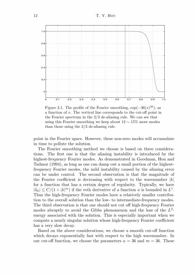
12 T. Y. Hou
0 0.1 0.2 0.3 0.4 0.5 0.6 0.7 0.8 0.9 1.0
0
0.2
0.4
0.6
0.8
1.0
Figure 2.1. The profile of the Fourier smoothing, exp(−36(x)36), asa function of x. The vertical line corresponds to the cut-off point inthe Fourier spectrum in the 2/3 de-aliasing rule. We can see thatusing this Fourier smoothing we keep about 12 ∼ 15% more modesthan those using the 2/3 de-aliasing rule.
point in the Fourier space. However, these non-zero modes will accumulatein time to pollute the solution.
The Fourier smoothing method we choose is based on three considera-tions. The first one is that the aliasing instability is introduced by thehighest-frequency Fourier modes. As demonstrated in Goodman, Hou andTadmor (1994), as long as one can damp out a small portion of the highest-frequency Fourier modes, the mild instability caused by the aliasing errorcan be under control. The second observation is that the magnitude ofthe Fourier coefficient is decreasing with respect to the wavenumber |k|for a function that has a certain degree of regularity. Typically, we have|uk| ≤ C/(1 + |k|m) if the mth derivative of a function u is bounded in L1.Thus the high-frequency Fourier modes have a relatively smaller contribu-tion to the overall solution than the low- to intermediate-frequency modes.The third observation is that one should not cut off high-frequency Fouriermodes abruptly to avoid the Gibbs phenomenon and the loss of the L2-energy associated with the solution. This is especially important when wecompute a nearly singular solution whose high-frequency Fourier coefficienthas a very slow decay.
Based on the above considerations, we choose a smooth cut-off functionwhich decays exponentially fast with respect to the high wavenumber. Inour cut-off function, we choose the parameters α = 36 and m = 36. These
Blow-up or no blow-up? 13
two parameters are chosen to achieve two objectives. (i) When |k| is closeto N , the cut-off function reaches machine precision, i.e., 10−16. (ii) Thecut-off function remains very close to 1 for |k| < 4N/5, and decays rapidlyand smoothly to zero beyond |k| = 4N/5. In Figure 2.1, we plot the cut-off function ρ(x) as a function of x. The cut-off function used by the 2/3de-aliasing rule is plotted on top of the cut-off function used by the Fouriersmoothing method. We can see that the Fourier smoothing method keepsabout 12 ∼ 15% more modes than the 2/3 de-aliasing method. In this paper,we will demonstrate by our numerical experiments that the extra modes wekeep by the Fourier smoothing method give an accurate approximation ofthe correct high-frequency Fourier modes.
We have performed a sequence of resolution studies with the largest reso-lution being N = 16384 (Hou and Li 2007). Our extensive numerical resultsdemonstrate that the pseudo-spectral method with the high-order Fouriersmoothing (the Fourier smoothing method for short) gives a much moreaccurate approximation than the pseudo-spectral method with the 2/3 de-aliasing rule (the 2/3 de-aliasing method for short). One of the interestingobservations is that the unfiltered high-frequency coefficients in the Fouriersmoothing method approximate accurately the corresponding exact Fouriercoefficients. Moreover, we observe that the Fourier smoothing method cap-tures about 12 ∼ 15% more effective Fourier modes than the 2/3 de-aliasingmethod in each dimension: see Figure 2.2. The gain is even higher for the 3DEuler equations since the number of effective modes in the Fourier smooth-ing method is higher in three dimensions. Further, we find that the errorproduced by the Fourier smoothing method is highly localized near the re-gion where the solution is most singular. In fact, the pointwise error decaysexponentially fast away from the location of the shock singularities. On theother hand, the error produced by the 2/3 de-aliasing method spreads outto the entire domain as we approach the singularity time: see Figure 2.3.
2.5. The high-resolution 3D Euler computations of Hou and Li (2006, 2007 )
Hou and Li (2006) performed high-resolution computations of the 3D Eulerequations using the initial data for the two antiparallel vortex tubes. Theyused the same initial condition whose analytic formula was given by Kerr(see Section III of Kerr (1993), and also Hou and Li (2006) for correctionsof some typos in the description of the initial condition in Kerr (1993)).However, there was some minor difference between their discretization andKerr’s discretization. Hou and Li used a pseudo-spectral discretization in allthree directions, while Kerr used a pseudo-spectral discretization only in thex- and y-directions and used a Chebyshev discretization in the z-direction.Based on the results of early tests, positive vorticity in the symmetry planewas imposed in the initial condition of Kerr (1993). How this was imposed
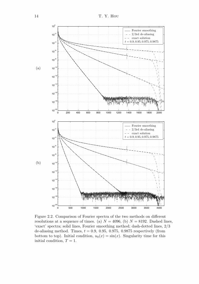
14 T. Y. Hou
(a)
0 200 400 600 800 1000 1200 1400 1600 1800 200010
−20
10−18
10−16
10−14
10−12
10−10
10−8
10−6
10−4
10−2
100
Fourier smoothing2/3rd de-aliasingexact solution
t = 0.9, 0.95, 0.975, 0.9875
(b)
0 500 1000 1500 2000 2500 3000 3500 400010
−20
10−18
10−16
10−14
10−12
10−10
10−8
10−6
10−4
10−2
100
Fourier smoothing2/3rd de-aliasingexact solution
t = 0.9, 0.95, 0.975, 0.9875
Figure 2.2. Comparison of Fourier spectra of the two methods on differentresolutions at a sequence of times. (a) N = 4096, (b) N = 8192. Dashed lines,‘exact’ spectra; solid lines, Fourier smoothing method; dash-dotted lines, 2/3de-aliasing method. Times, t = 0.9, 0.95, 0.975, 0.9875 respectively (frombottom to top). Initial condition, u0(x) = sin(x). Singularity time for thisinitial condition, T = 1.
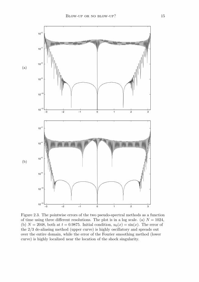
Blow-up or no blow-up? 15
(a)
−3 −2 −1 0 1 2 310
−12
10−10
10−8
10−6
10−4
10−2
(b)
−3 −2 −1 0 1 2 310
−12
10−10
10−8
10−6
10−4
10−2
Figure 2.3. The pointwise errors of the two pseudo-spectral methods as a functionof time using three different resolutions. The plot is in a log scale. (a) N = 1024,(b) N = 2048, both at t = 0.9875. Initial condition, u0(x) = sin(x). The error ofthe 2/3 de-aliasing method (upper curve) is highly oscillatory and spreads outover the entire domain, while the error of the Fourier smoothing method (lowercurve) is highly localized near the location of the shock singularity.
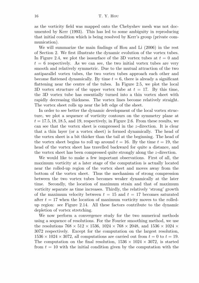
16 T. Y. Hou
as the vorticity field was mapped onto the Chebyshev mesh was not doc-umented by Kerr (1993). This has led to some ambiguity in reproducingthat initial condition which is being resolved by Kerr’s group (private com-munication).
We will summarize the main findings of Hou and Li (2006) in the restof Section 2. We first illustrate the dynamic evolution of the vortex tubes.In Figure 2.4, we plot the isosurface of the 3D vortex tubes at t = 0 andt = 6 respectively. As we can see, the two initial vortex tubes are verysmooth and relatively symmetric. Due to the mutual attraction of the twoantiparallel vortex tubes, the two vortex tubes approach each other andbecome flattened dynamically. By time t = 6, there is already a significantflattening near the centre of the tubes. In Figure 2.5, we plot the local3D vortex structure of the upper vortex tube at t = 17. By this time,the 3D vortex tube has essentially turned into a thin vortex sheet withrapidly decreasing thickness. The vortex lines become relatively straight.The vortex sheet rolls up near the left edge of the sheet.
In order to see better the dynamic development of the local vortex struc-ture, we plot a sequence of vorticity contours on the symmetry plane att = 17.5, 18, 18.5, and 19, respectively, in Figure 2.6. From these results, wecan see that the vortex sheet is compressed in the z-direction. It is clearthat a thin layer (or a vortex sheet) is formed dynamically. The head ofthe vortex sheet is a bit thicker than the tail at the beginning. The head ofthe vortex sheet begins to roll up around t = 16. By the time t = 19, thehead of the vortex sheet has travelled backward for quite a distance, andthe vortex sheet has been compressed quite strongly along the z-direction.
We would like to make a few important observations. First of all, themaximum vorticity at a later stage of the computation is actually locatednear the rolled-up region of the vortex sheet and moves away from thebottom of the vortex sheet. Thus the mechanism of strong compressionbetween the two vortex tubes becomes weaker dynamically at the latertime. Secondly, the location of maximum strain and that of maximumvorticity separate as time increases. Thirdly, the relatively ‘strong’ growthof the maximum velocity between t = 15 and t = 17 becomes saturatedafter t = 17 when the location of maximum vorticity moves to the rolled-up region: see Figure 2.14. All these factors contribute to the dynamicdepletion of vortex stretching.
We now perform a convergence study for the two numerical methodsusing a sequence of resolutions. For the Fourier smoothing method, we usethe resolutions 768 × 512 × 1536, 1024 × 768 × 2048, and 1536 × 1024 ×3072 respectively. Except for the computation on the largest resolution,1536 × 1024 × 3072, all computations are carried out from t = 0 to t = 19.The computation on the final resolution, 1536 × 1024 × 3072, is startedfrom t = 10 with the initial condition given by the computation with the
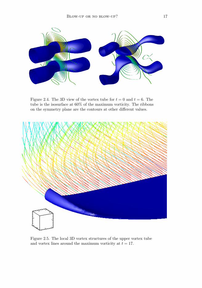
Blow-up or no blow-up? 17
Figure 2.4. The 3D view of the vortex tube for t = 0 and t = 6. Thetube is the isosurface at 60% of the maximum vorticity. The ribbonson the symmetry plane are the contours at other different values.
Figure 2.5. The local 3D vortex structures of the upper vortex tubeand vortex lines around the maximum vorticity at t = 17.
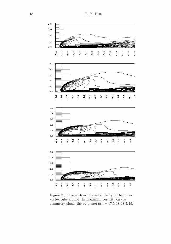
18 T. Y. Hou
Figure 2.6. The contour of axial vorticity of the uppervortex tube around the maximum vorticity on thesymmetry plane (the xz-plane) at t = 17.5, 18, 18.5, 19.
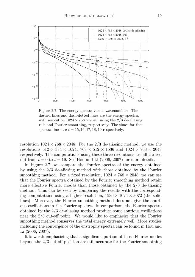
Blow-up or no blow-up? 19
0 200 400 600 800 1000 120010
−30
10−25
10−20
10−15
10−10
10−5
100
1024 × 768 × 2048, 2/3rd de-aliasing1024 × 768 × 2048, FS1536 × 1024 × 3072, FS
Figure 2.7. The energy spectra versus wavenumbers. Thedashed lines and dash-dotted lines are the energy spectra,with resolution 1024 × 768 × 2048, using the 2/3 de-aliasingrule and Fourier smoothing, respectively. The times for thespectra lines are t = 15, 16, 17, 18, 19 respectively.
resolution 1024 × 768 × 2048. For the 2/3 de-aliasing method, we use theresolutions 512 × 384 × 1024, 768 × 512 × 1536 and 1024 × 768 × 2048respectively. The computations using these three resolutions are all carriedout from t = 0 to t = 19. See Hou and Li (2006, 2007) for more details.
In Figure 2.7, we compare the Fourier spectra of the energy obtainedby using the 2/3 de-aliasing method with those obtained by the Fouriersmoothing method. For a fixed resolution, 1024 × 768 × 2048, we can seethat the Fourier spectra obtained by the Fourier smoothing method retainmore effective Fourier modes than those obtained by the 2/3 de-aliasingmethod. This can be seen by comparing the results with the correspond-ing computations using a higher resolution, 1536 × 1024 × 3072 (the solidlines). Moreover, the Fourier smoothing method does not give the spuri-ous oscillations in the Fourier spectra. In comparison, the Fourier spectraobtained by the 2/3 de-aliasing method produce some spurious oscillationsnear the 2/3 cut-off point. We would like to emphasize that the Fouriersmoothing method conserves the total energy extremely well. More studiesincluding the convergence of the enstrophy spectra can be found in Hou andLi (2006, 2007).
It is worth emphasizing that a significant portion of those Fourier modesbeyond the 2/3 cut-off position are still accurate for the Fourier smoothing
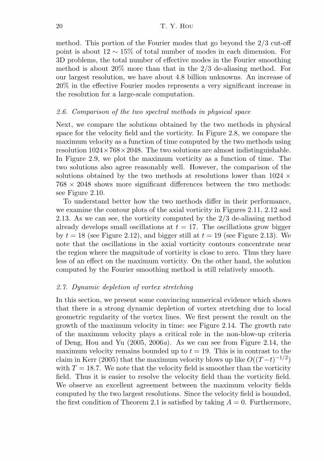
20 T. Y. Hou
method. This portion of the Fourier modes that go beyond the 2/3 cut-offpoint is about 12 ∼ 15% of total number of modes in each dimension. For3D problems, the total number of effective modes in the Fourier smoothingmethod is about 20% more than that in the 2/3 de-aliasing method. Forour largest resolution, we have about 4.8 billion unknowns. An increase of20% in the effective Fourier modes represents a very significant increase inthe resolution for a large-scale computation.
2.6. Comparison of the two spectral methods in physical space
Next, we compare the solutions obtained by the two methods in physicalspace for the velocity field and the vorticity. In Figure 2.8, we compare themaximum velocity as a function of time computed by the two methods usingresolution 1024×768×2048. The two solutions are almost indistinguishable.In Figure 2.9, we plot the maximum vorticity as a function of time. Thetwo solutions also agree reasonably well. However, the comparison of thesolutions obtained by the two methods at resolutions lower than 1024 ×768 × 2048 shows more significant differences between the two methods:see Figure 2.10.
To understand better how the two methods differ in their performance,we examine the contour plots of the axial vorticity in Figures 2.11, 2.12 and2.13. As we can see, the vorticity computed by the 2/3 de-aliasing methodalready develops small oscillations at t = 17. The oscillations grow biggerby t = 18 (see Figure 2.12), and bigger still at t = 19 (see Figure 2.13). Wenote that the oscillations in the axial vorticity contours concentrate nearthe region where the magnitude of vorticity is close to zero. Thus they haveless of an effect on the maximum vorticity. On the other hand, the solutioncomputed by the Fourier smoothing method is still relatively smooth.
2.7. Dynamic depletion of vortex stretching
In this section, we present some convincing numerical evidence which showsthat there is a strong dynamic depletion of vortex stretching due to localgeometric regularity of the vortex lines. We first present the result on thegrowth of the maximum velocity in time: see Figure 2.14. The growth rateof the maximum velocity plays a critical role in the non-blow-up criteriaof Deng, Hou and Yu (2005, 2006a). As we can see from Figure 2.14, themaximum velocity remains bounded up to t = 19. This is in contrast to theclaim in Kerr (2005) that the maximum velocity blows up like O((T−t)−1/2)with T = 18.7. We note that the velocity field is smoother than the vorticityfield. Thus it is easier to resolve the velocity field than the vorticity field.We observe an excellent agreement between the maximum velocity fieldscomputed by the two largest resolutions. Since the velocity field is bounded,the first condition of Theorem 2.1 is satisfied by taking A = 0. Furthermore,
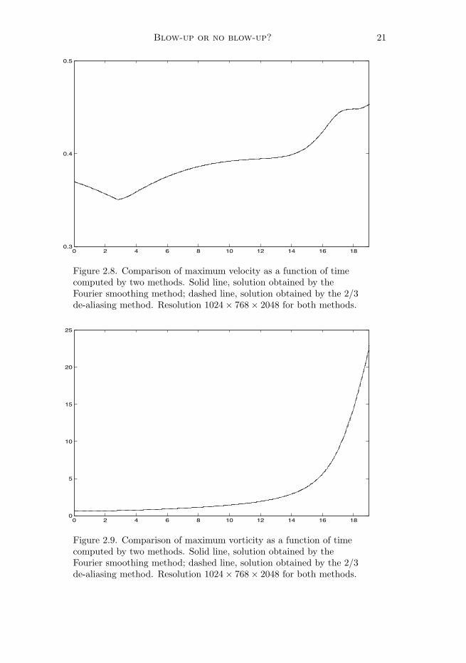
Blow-up or no blow-up? 21
0 2 4 6 8 10 12 14 16 180.3
0.4
0.5
Figure 2.8. Comparison of maximum velocity as a function of timecomputed by two methods. Solid line, solution obtained by theFourier smoothing method; dashed line, solution obtained by the 2/3de-aliasing method. Resolution 1024 × 768 × 2048 for both methods.
0 2 4 6 8 10 12 14 16 180
5
10
15
20
25
Figure 2.9. Comparison of maximum vorticity as a function of timecomputed by two methods. Solid line, solution obtained by theFourier smoothing method; dashed line, solution obtained by the 2/3de-aliasing method. Resolution 1024 × 768 × 2048 for both methods.
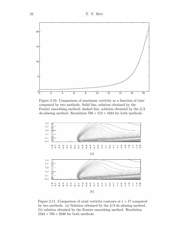
22 T. Y. Hou
0 2 4 6 8 10 12 14 16 180
5
10
15
20
Figure 2.10. Comparison of maximum vorticity as a function of timecomputed by two methods. Solid line, solution obtained by theFourier smoothing method; dashed line, solution obtained by the 2/3de-aliasing method. Resolution 768 × 512 × 1024 for both methods.
(a)
(b)
Figure 2.11. Comparison of axial vorticity contours at t = 17 computedby two methods. (a) Solution obtained by the 2/3 de-aliasing method,(b) solution obtained by the Fourier smoothing method. Resolution1024 × 768 × 2048 for both methods.
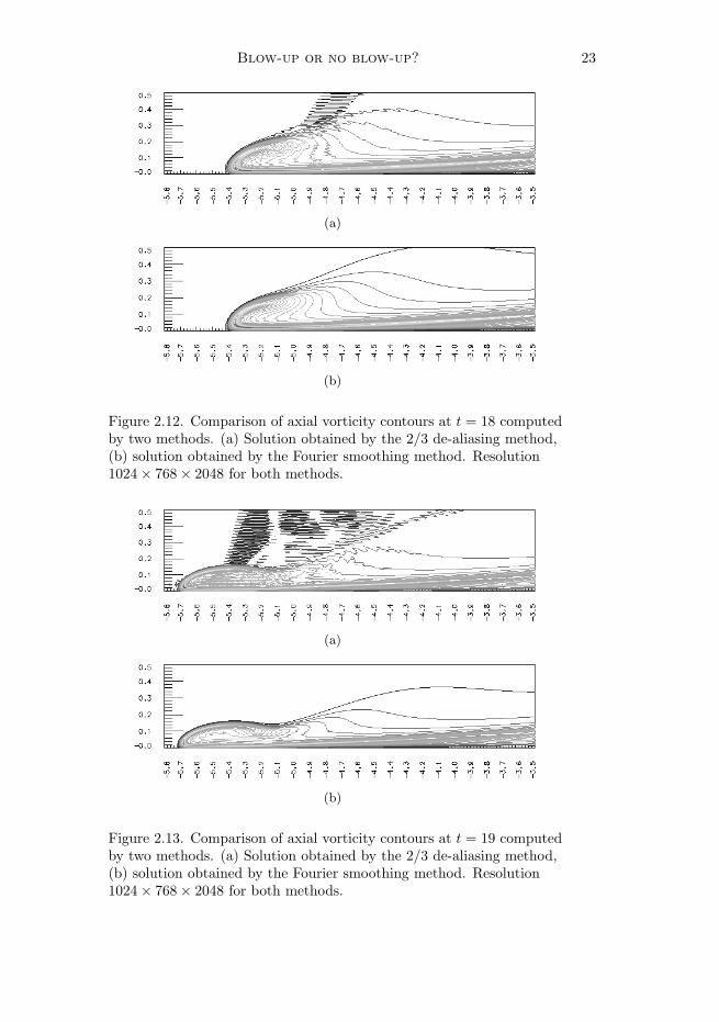
Blow-up or no blow-up? 23
(a)
(b)
Figure 2.12. Comparison of axial vorticity contours at t = 18 computedby two methods. (a) Solution obtained by the 2/3 de-aliasing method,(b) solution obtained by the Fourier smoothing method. Resolution1024 × 768 × 2048 for both methods.
(a)
(b)
Figure 2.13. Comparison of axial vorticity contours at t = 19 computedby two methods. (a) Solution obtained by the 2/3 de-aliasing method,(b) solution obtained by the Fourier smoothing method. Resolution1024 × 768 × 2048 for both methods.
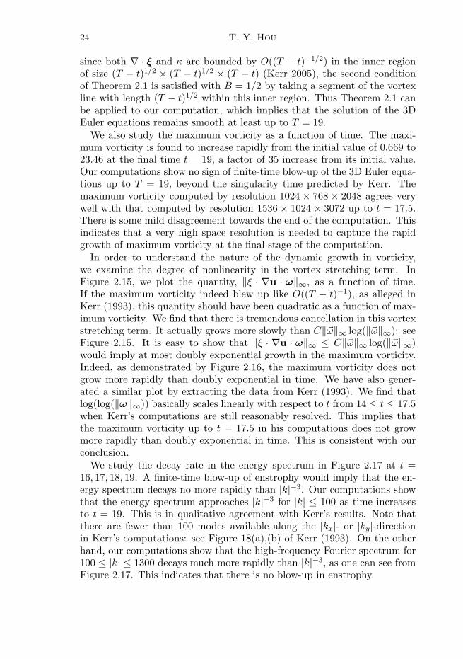
24 T. Y. Hou
since both ∇ · ξ and κ are bounded by O((T − t)−1/2) in the inner regionof size (T − t)1/2 × (T − t)1/2 × (T − t) (Kerr 2005), the second conditionof Theorem 2.1 is satisfied with B = 1/2 by taking a segment of the vortexline with length (T − t)1/2 within this inner region. Thus Theorem 2.1 canbe applied to our computation, which implies that the solution of the 3DEuler equations remains smooth at least up to T = 19.
We also study the maximum vorticity as a function of time. The maxi-mum vorticity is found to increase rapidly from the initial value of 0.669 to23.46 at the final time t = 19, a factor of 35 increase from its initial value.Our computations show no sign of finite-time blow-up of the 3D Euler equa-tions up to T = 19, beyond the singularity time predicted by Kerr. Themaximum vorticity computed by resolution 1024 × 768 × 2048 agrees verywell with that computed by resolution 1536 × 1024 × 3072 up to t = 17.5.There is some mild disagreement towards the end of the computation. Thisindicates that a very high space resolution is needed to capture the rapidgrowth of maximum vorticity at the final stage of the computation.
In order to understand the nature of the dynamic growth in vorticity,we examine the degree of nonlinearity in the vortex stretching term. InFigure 2.15, we plot the quantity, ‖ξ · ∇u · ω‖∞, as a function of time.If the maximum vorticity indeed blew up like O((T − t)−1), as alleged inKerr (1993), this quantity should have been quadratic as a function of max-imum vorticity. We find that there is tremendous cancellation in this vortexstretching term. It actually grows more slowly than C‖ω‖∞ log(‖ω‖∞): seeFigure 2.15. It is easy to show that ‖ξ · ∇u · ω‖∞ ≤ C‖ω‖∞ log(‖ω‖∞)would imply at most doubly exponential growth in the maximum vorticity.Indeed, as demonstrated by Figure 2.16, the maximum vorticity does notgrow more rapidly than doubly exponential in time. We have also gener-ated a similar plot by extracting the data from Kerr (1993). We find thatlog(log(‖ω‖∞)) basically scales linearly with respect to t from 14 ≤ t ≤ 17.5when Kerr’s computations are still reasonably resolved. This implies thatthe maximum vorticity up to t = 17.5 in his computations does not growmore rapidly than doubly exponential in time. This is consistent with ourconclusion.
We study the decay rate in the energy spectrum in Figure 2.17 at t =16, 17, 18, 19. A finite-time blow-up of enstrophy would imply that the en-ergy spectrum decays no more rapidly than |k|−3. Our computations showthat the energy spectrum approaches |k|−3 for |k| ≤ 100 as time increasesto t = 19. This is in qualitative agreement with Kerr’s results. Note thatthere are fewer than 100 modes available along the |kx|- or |ky|-directionin Kerr’s computations: see Figure 18(a),(b) of Kerr (1993). On the otherhand, our computations show that the high-frequency Fourier spectrum for100 ≤ |k| ≤ 1300 decays much more rapidly than |k|−3, as one can see fromFigure 2.17. This indicates that there is no blow-up in enstrophy.
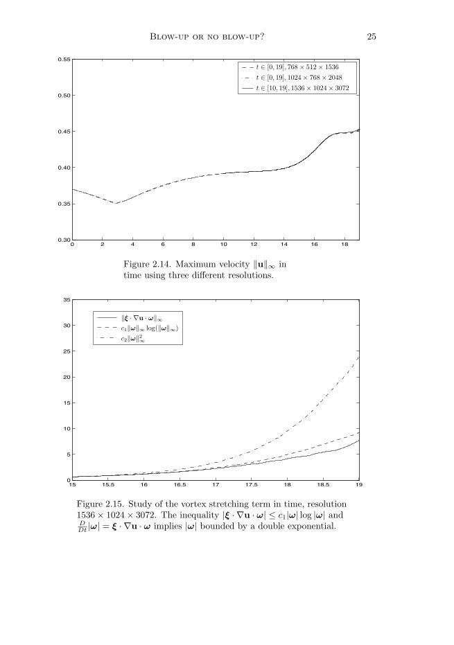
Blow-up or no blow-up? 25
0 2 4 6 8 10 12 14 16 180.30
0.35
0.40
0.45
0.50
0.55
t ∈ [0, 19], 768 × 512 × 1536
t ∈ [0, 19], 1024 × 768 × 2048
t ∈ [10, 19], 1536 × 1024 × 3072
Figure 2.14. Maximum velocity ‖u‖∞ intime using three different resolutions.
15 15.5 16 16.5 17 17.5 18 18.5 190
5
10
15
20
25
30
35
‖ξ · ∇u · ω‖∞c1‖ω‖∞ log(‖ω‖∞)c2‖ω‖2
∞
Figure 2.15. Study of the vortex stretching term in time, resolution1536 × 1024 × 3072. The inequality |ξ · ∇u · ω| ≤ c1|ω| log |ω| andDDt |ω| = ξ · ∇u · ω implies |ω| bounded by a double exponential.
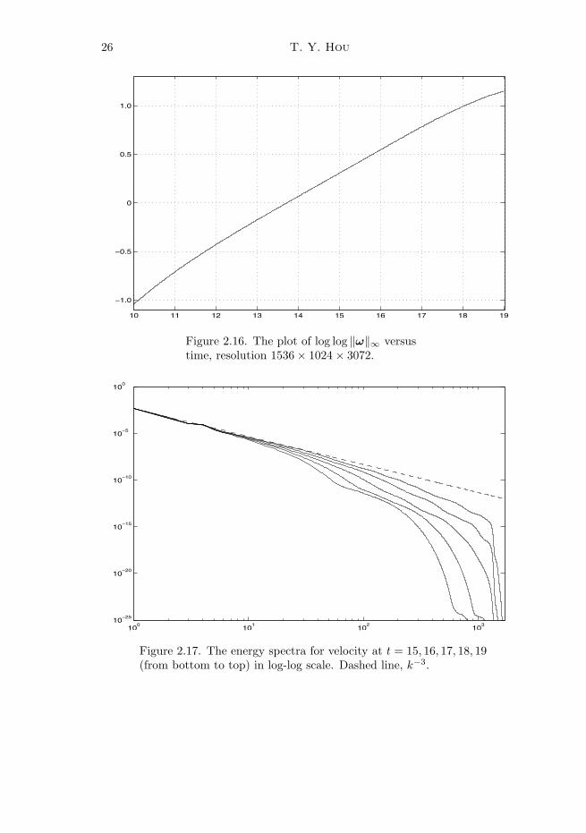
26 T. Y. Hou
10 11 12 13 14 15 16 17 18 19
−1.0
−0.5
0
0.5
1.0
Figure 2.16. The plot of log log ‖ω‖∞ versustime, resolution 1536 × 1024 × 3072.
100
101
102
103
10−25
10−20
10−15
10−10
10−5
100
Figure 2.17. The energy spectra for velocity at t = 15, 16, 17, 18, 19(from bottom to top) in log-log scale. Dashed line, k−3.
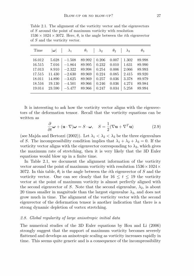
Blow-up or no blow-up? 27
Table 2.1. The alignment of the vorticity vector and the eigenvectorsof S around the point of maximum vorticity with resolution1536 × 1024 × 3072. Here, θi is the angle between the ith eigenvectorof S and the vorticity vector.
Time |ω| λ1 θ1 λ2 θ2 λ3 θ3
16.012 5.628 −1.508 89.992 0.206 0.007 1.302 89.99816.515 7.016 −1.864 89.995 0.232 0.010 1.631 89.99017.013 8.910 −2.322 89.998 0.254 0.006 2.066 89.99317.515 11.430 −2.630 89.969 0.224 0.085 2.415 89.92018.011 14.890 −3.625 89.969 0.257 0.036 3.378 89.97918.516 19.130 −4.501 89.966 0.246 0.036 4.274 89.98419.014 23.590 −5.477 89.966 0.247 0.034 5.258 89.994
It is interesting to ask how the vorticity vector aligns with the eigenvec-tors of the deformation tensor. Recall that the vorticity equations can bewritten as
∂
∂tω + (u · ∇)ω = S · ω, S =
12(∇u + ∇Tu) (2.9)
(see Majda and Bertozzi (2002)). Let λ1 < λ2 < λ3 be the three eigenvaluesof S. The incompressibility condition implies that λ1 + λ2 + λ3 = 0. If thevorticity vector aligns with the eigenvector corresponding to λ3, which givesthe maximum rate of stretching, then it is very likely that the 3D Eulerequations would blow up in a finite time.
In Table 2.1, we document the alignment information of the vorticityvector around the point of maximum vorticity with resolution 1536×1024×3072. In this table, θi is the angle between the ith eigenvector of S and thevorticity vector. One can see clearly that for 16 ≤ t ≤ 19 the vorticityvector at the point of maximum vorticity is almost perfectly aligned withthe second eigenvector of S. Note that the second eigenvalue, λ2, is about20 times smaller in magnitude than the largest eigenvalue λ3, and does notgrow much in time. The alignment of the vorticity vector with the secondeigenvector of the deformation tensor is another indication that there is astrong dynamic depletion of vortex stretching.
2.8. Global regularity of large anisotropic initial data
The numerical studies of the 3D Euler equations by Hou and Li (2006)strongly suggest that the support of maximum vorticity becomes severelyflattened and develops an anisotropic scaling as vorticity increases rapidly intime. This seems quite generic and is a consequence of the incompressibility
28 T. Y. Hou
and the Lagrangian structure of the vorticity equation. Convection playsan essential role in producing this anisotropic structure of the solution.Motivated by the desire to understand how the local anisotropic structureof the solution near the support of maximum vorticity may lead to thedepletion of vortex stretching, Hou, Lei and Li (2008) recently studied the3D axisymmetric Navier–Stokes equations with large anisotropic data. Theyproved the global regularity of the 3D Navier–Stokes equations for a familyof large anisotropic initial data. Moreover, they obtained a global bound ofthe solution in terms of its initial data in some Lp-norm. Their results alsorevealed some interesting dynamic growth behaviour of the solution due tothe interaction between the axial vorticity and the the derivative of vorticity.
Specifically, let uθ and ωθ be the angular velocity and vorticity compo-nents of the 3D axisymmetric Navier–Stokes equations. They consideredinitial data for uθ and ωθ that have the following scaling property:
uθ(r, z, 0) =1
ε1−δU0(εr, z), ωθ(r, z, 0) =
1ε1−δ
W0(εr, z), (2.10)
where r =√x2 + y2, δ and ε are some small positive parameters, and the
rescaled profiles U0/r andW0/r are bounded in L2p and L2q, respectively, forsome p and q with p = 2q; note that uθ and ωθ must satisfy a compatibilitycondition: uθ|r=0 = 0 = ωθ|r=0 (Liu and Wang 2006). We remark thatthese initial data are not small. In fact, we have
‖u0‖L2(R2×[0,1])‖∇u0‖L2(R2×[0,1]) =C0
ε4−2δ 1,
for ε small, where u0 is the initial velocity vector. Thus the classical regular-ity analysis for small initial data does not apply to these sets of anisotropicinitial data.
Hou, Lei and Li (2008) proved the global regularity of the 3D axisym-metric Navier–Stokes equations for initial data (2.10) by exploring the an-isotropic structure of the solution for ε small. They also obtained a globalbound on ‖uθ/r‖L2p and ‖ωθ/r‖L2q in terms of their initial data. Notethat by using the scaling invariance property of the Navier–Stokes equa-tions, their global regularity result also applies to the following rescaledinitial data:
uθ(r, z, 0) =1
ε2−δU0
(
r,z
ε
)
, ωθ(r, z, 0) =1
ε3−δW0
(
r,z
ε
)
, (2.11)
and
uθ(r, z, 0) =1εU0
(r
ε1−δ,z
ε
)
, ωθ(r, z, 0) =1ε2W0
(r
ε1−δ,z
ε
)
. (2.12)
Note that the parameters ε in the initial data (2.10)–(2.11) and δ in (2.12)measure the degree of anisotropy of the initial data. If δ = 0, then the
Blow-up or no blow-up? 29
initial data (2.12) become isotropic, i.e.,
u0(x, y, z) =1εU0
(x
ε,y
ε,z
ε
)
.
Their analysis would break down when there is no anisotropic scaling inthe initial data, i.e., δ = 0. Clearly, if the analysis could be extended tothe case of δ = 0, one would prove the global regularity of the 3D axisym-metric Navier–Stokes equations for general initial data by using the scalinginvariance property of the Navier–Stokes equations. It is interesting to notethat by using an anisotropic scaling of the initial data, we turn the globalregularity of the 3D Navier–Stokes equations into a critical case of δ = 0.
We remark that the global regularity results of Hou, Lei and Li (2008)were obtained on a regular size domain, R2 × [0, 1], for initial data (2.10).In this sense, their results are different from those global regularity resultsobtained for a thin domain, Ωε = Q1 × [0, ε] with Q1 being a bounded do-main in R2. The global regularity of the 3D Navier–Stokes equations ina thin domain of the form Ωε has been studied by Raugel and Sell in aseries of papers (Raugel and Sell 1993a, 1994, 1993b). They proved theglobal regularity of the 3D Navier–Stokes equations under the assumptionthat ‖∇u0‖2
L2(Ωε)≤ C0 ln 1
ε . This is an improvement over the classical globalregularity result for small data, which requires ‖∇u0‖2
L2(Ωε)≤ C∗ε (Raugel
and Sell 1993a). One may interpret the global regularity result of Hou,Lei and Li with initial data (2.11) as a result on a generalized thin do-main. Note that the initial data given by (2.11) satisfy the following bound:‖∇u0‖2
L2(Ωε)= C0ε
−5+2δ (here δ > 0 can be made arbitrarily small), whichis much larger than the corresponding bound C0 ln 1
ε required by the globalregularity analysis of Raugel and Sell (1993a, 1994, 1993b).
3. Dynamic stability of 3D Navier–Stokes equations
The axisymmetric 3D Navier–Stokes equation with swirl is perhaps the sim-plest form of the 3D Navier–Stokes equations, yet still retains the most es-sential difficulties of the 3D Navier–Stokes equations. It has attracted a lotof attention in recent years. Although some partial progress has been madein studying the global regularity of the axisymmetric Navier–Stokes equa-tions with swirl using energy estimates (see, e.g., Chae and Lee (2002) andreferences cited there), the question of global regularity for general initialdata is still an open question.
Hou and Li (2008a) studied the dynamic stability of the axisymmetricNavier–Stokes equations with swirl via a new 1D model. This model isderived from the axisymmetric Navier–Stokes equations along the symmetryaxis. Surprisingly, this model is an exact reduction of the 3D axisymmetric

30 T. Y. Hou
Navier–Stokes equations along the symmetry axis. It captures the essentialnonlinear features of the 3D Navier–Stokes equations. One of the importantfindings by Hou and Li (2008a) was that the convection term plays anessential role in cancelling some of the vortex stretching terms. Specifically,they found a positive Lyapunov function which satisfies a new conservationlaw and a maximum principle. This holds for both the viscous and inviscidcases. This a priori pointwise estimate plays a critical role in obtainingnonlinear stability and global regularity of the 1D model. Using this a prioriestimate, they proved global regularity of the 3D Navier–Stokes equationsfor a family of large data, which can experience large transient dynamicgrowth but remain smooth for all times.
It is worth emphasizing that such subtle dynamic stability properties ofthe 3D Navier–Stokes equations would have been completely missed by usingthe traditional energy estimates. Traditional energy estimates are too crudeto capture some of the most essential properties of the 3D incompressibleNavier–Stokes equations. To illustrate its limitations, we briefly review howthe energy estimates are used in proving global regularity of the 3D Navier–Stokes equations.
For incompressible Navier–Stokes equations, one of the most importanta priori estimates is the energy identity. More precisely, for any strongsolution u, we have
12
ddt
∫|u|2 dx + ν
∫|∇u|2 dx = 0, (3.1)
by observing∫
u·(u·∇u) dx = −12
∫(∇·u)|u|2 dx = 0, since u is divergence-
free. Unfortunately, this energy identity is not strong enough to rule outfinite-time singularities. To prove global regularity, we need to obtain con-trol in a stronger norm, either in ‖u‖Lp with p ≥ 3 or in ‖ω‖L2 . To illustratethe main difficulty of the traditional energy estimates, let us perform energyestimates for the vorticity equation:
12
ddt
∫|ω|2 dx + ν
∫|∇ω|2 dx =
∫ω · ∇u · ω dx. (3.2)
Again, the convection term does not contribute to the L2-norm of vorticity(or any Lp-norm with p > 1). The main difficulty is to control the vortexstretching term. Using the Sobolev embedding theory, one can show that
∫ω · ∇u · ω dx ≤ Cν
(∫|ω|2 dx
)3
+ν
2
∫|∇ω|2 dx, (3.3)
which can not be improved. This implies that
12
ddt
∫|ω|2 dx +
ν
2
∫|∇ω|2 dx ≤ Cν
(∫|ω|2 dx
)3
. (3.4)
Blow-up or no blow-up? 31
Unfortunately, the above estimate does not imply global regularity for largedata even if we use the energy identity (3.1). However, the estimate (3.4)can be used to obtain global regularity for small initial data. To see this,we substitute the following interpolation inequality,
(∫|ω|2 dx
)2
= ‖ω‖4L2 ≤ C0‖u‖2
L2‖∇ω‖2L2 , (3.5)
into (3.4) to obtain
12
ddt
‖ω‖2L2 ≤
(
CνC0‖u‖2L2‖ω‖2
L2 − ν
2
)
‖∇ω‖2L2 ≤ 0, (3.6)
provided that
CνC0‖u0‖2L2‖ω0‖2
L2 ≤ ν
2. (3.7)
Since ‖u(t)‖2L2 ≤ ‖u0‖2
L2 for all t, condition (3.7) and inequality (3.6) implythat ‖ω(t)‖2
L2 ≤ ‖ω0‖2L2 for all times. Note that ‖ω0‖2
L2 = ‖∇u0‖2L2 . Thus
we can also replace (3.7) by
CνC0‖u0‖2L2‖∇u0‖2
L2 ≤ ν
2. (3.8)
Due to the incompressibility condition, convection plays no role in theenergy estimate. The same estimate can be also applied to the followingnonlinear diffusion equation:
wt = w2 + ν∆w. (3.9)
An energy estimate gives
12
ddt
∫|w|2 dx + ν
∫|∇w|2 dx =
∫w3 dx. (3.10)
Using an embedding inequality similar to (3.3), we get
12
ddt
∫|w|2 dx +
ν
2
∫|∇w|2 dx ≤ Cν
(∫|w|2 dx
)3
, (3.11)
which is identical to (3.4).However, it is well known that (3.9) can develop a finite-time isotropic
self-similar blow-up solution, which does not violate the energy identity(3.1), in the sense that
∫ T0 ‖w(t)‖2
L2 dt <∞. The above analysis shows thatenergy estimates can not distinguish a nonlinear diffusion equation, whichhas a finite-time blow-up solution, from the 3D Navier–Stokes equations,which have completely different physical properties and may not necessarilyblow up in finite time.
32 T. Y. Hou
3.1. Reformulation of 3D axisymmetric Navier–Stokes equations
Consider the 3D axisymmetric incompressible Navier–Stokes equations
uθt + uruθ
r + uzuθz = ν
(
∇2 − 1r2
)
uθ − 1ruruθ, (3.12)
ωθt + urωθ
r + uzωθz = ν
(
∇2 − 1r2
)
ωθ +1r
((uθ)2
)z+
1rurωθ, (3.13)
−(
∇2 − 1r2
)
ψθ = ωθ, (3.14)
where r =√x2 + y2, uθ, ωθ and ψθ are the angular components of the
velocity, vorticity and stream function respectively, and
ur = −(ψθ)z uz =1r(rψθ)r.
Note that equations (3.12)–(3.14) completely determine the evolution of the3D axisymmetric Navier–Stokes equations.
Hou and Li (2008a) introduced the following new variables,
u1 = uθ/r, ω1 = ωθ/r, ψ1 = ψθ/r, (3.15)
and derived the following equivalent system that governs the dynamics ofu1, ω1 and ψ1:
∂tu1 + ur∂ru1 + uz∂zu1 = ν
(
∂2r +
3r∂r + ∂2
z
)
u1 + 2u1ψ1z, (3.16a)
∂tω1 + ur∂rω1 + uz∂zω1 = ν
(
∂2r +
3r∂r + ∂2
z
)
ω1 + (u21)z, (3.16b)
−(
∂2r +
3r∂r + ∂2
z
)
ψ1 = ω1, (3.16c)
where ur = −rψ1z, uz = 2ψ1+rψ1r. Liu and Wang (2006) showed that if uis a smooth velocity field, then uθ, ωθ and ψθ must satisfy the compatibilitycondition uθ|r=0 = ωθ|r=0 = ψθ|r=0 = 0. Thus u1, ψ1 and ω1 are well definedas long as the solution remains smooth.
3.2. An exact 1D model for 3D Navier–Stokes equations
Hou and Li (2008a) derived an exact 1D model along the symmetry axisby assuming the solution is more singular along the z-direction than alongthe r-direction (i.e., the solution has an locally anisotropic scaling). Alongthe symmetry axis r = 0, we have ur = 0, uz = 2ψ1. Since the solution ismore singular along the z-direction, one can drop the derivatives along ther-direction to the leading order in the reformulated Navier–Stokes equations(note that 3
r∂r is of the same order as ∂2r ). This gives rise to the following
Blow-up or no blow-up? 33
1D model:
(u1)t + 2ψ1(u1)z = ν(u1)zz + 2(ψ1)zu1, (3.17)
(ω1)t + 2ψ1(ω1)z = ν(ω1)zz + (u21)z, (3.18)
−(ψ1)zz = ω1. (3.19)
Note that the system (3.17)–(3.19) is already a closed system. Let u = u1,v = −(ψ1)z, and ψ = ψ1. By integrating (3.18) with respect to z, one canfurther reduce the above system to
(u)t + 2ψ(u)z = ν(u)zz − 2vu, (3.20)
(v)t + 2ψ(v)z = ν(v)zz + (u)2 − (v)2 + c(t), (3.21)
where v = −(ψ)z, vz = ω, and c(t) is an integration constant to enforcethe mean of v equal to zero. If we assume that the solution is periodicwith respect to z with period 1, the integration constant c(t) is equal to3
∫ 10 (v)2 dz − ∫ 1
0 (u)2 dz.A surprising result is that the above 1D model is exact. This is stated in
the following theorem.
Theorem 3.1. Let u1, ψ1 and ω1 be the solution of the 1D model (3.17)–(3.19) and define
uθ(r, z, t) = ru1(z, t), ωθ(r, z, t) = rω1(z, t), ψθ(r, z, t) = rψ1(z, t).
Then (uθ(r, z, t), ωθ(r, z, t), ψθ(r, z, t)) is an exact solution of the 3D Navier–Stokes equations.
Theorem 3.1 tells us that the 1D model (3.17)–(3.19) preserves some es-sential nonlinear structure of the 3D axisymmetric Navier–Stokes equations.
3.3. Properties of the model equation
In this section, we will study some properties of the 1D model. We first con-sider the properties of some further simplified models obtained from theseequations. Both numerical and analytical studies are presented for thesesimplified models. Based on the understanding of the simplified models, weprove the global existence of the full 1D model.
The ODE modelTo start with, we consider an ODE model by ignoring the convection anddiffusion term:
(u)t = −2vu, (3.22)
(v)t = (u)2 − (v)2, (3.23)
with initial condition u(0) = u0 and v(0) = v0.
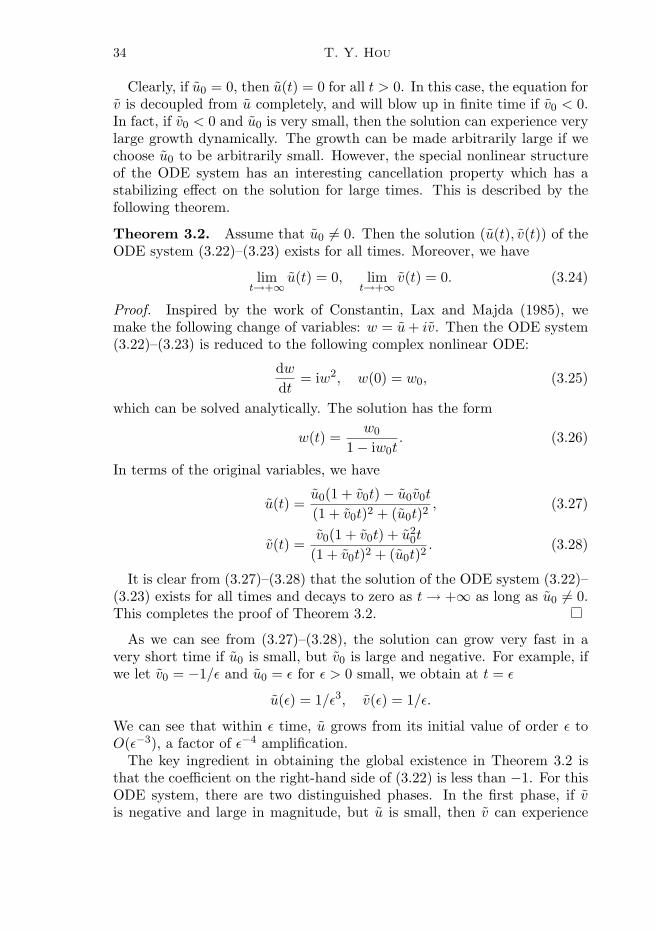
34 T. Y. Hou
Clearly, if u0 = 0, then u(t) = 0 for all t > 0. In this case, the equation forv is decoupled from u completely, and will blow up in finite time if v0 < 0.In fact, if v0 < 0 and u0 is very small, then the solution can experience verylarge growth dynamically. The growth can be made arbitrarily large if wechoose u0 to be arbitrarily small. However, the special nonlinear structureof the ODE system has an interesting cancellation property which has astabilizing effect on the solution for large times. This is described by thefollowing theorem.
Theorem 3.2. Assume that u0 = 0. Then the solution (u(t), v(t)) of theODE system (3.22)–(3.23) exists for all times. Moreover, we have
limt→+∞ u(t) = 0, lim
t→+∞ v(t) = 0. (3.24)
Proof. Inspired by the work of Constantin, Lax and Majda (1985), wemake the following change of variables: w = u+ iv. Then the ODE system(3.22)–(3.23) is reduced to the following complex nonlinear ODE:
dwdt
= iw2, w(0) = w0, (3.25)
which can be solved analytically. The solution has the form
w(t) =w0
1 − iw0t. (3.26)
In terms of the original variables, we have
u(t) =u0(1 + v0t) − u0v0t
(1 + v0t)2 + (u0t)2, (3.27)
v(t) =v0(1 + v0t) + u2
0t
(1 + v0t)2 + (u0t)2. (3.28)
It is clear from (3.27)–(3.28) that the solution of the ODE system (3.22)–(3.23) exists for all times and decays to zero as t→ +∞ as long as u0 = 0.This completes the proof of Theorem 3.2.
As we can see from (3.27)–(3.28), the solution can grow very fast in avery short time if u0 is small, but v0 is large and negative. For example, ifwe let v0 = −1/ε and u0 = ε for ε > 0 small, we obtain at t = ε
u(ε) = 1/ε3, v(ε) = 1/ε.
We can see that within ε time, u grows from its initial value of order ε toO(ε−3), a factor of ε−4 amplification.
The key ingredient in obtaining the global existence in Theorem 3.2 isthat the coefficient on the right-hand side of (3.22) is less than −1. For thisODE system, there are two distinguished phases. In the first phase, if vis negative and large in magnitude, but u is small, then v can experience
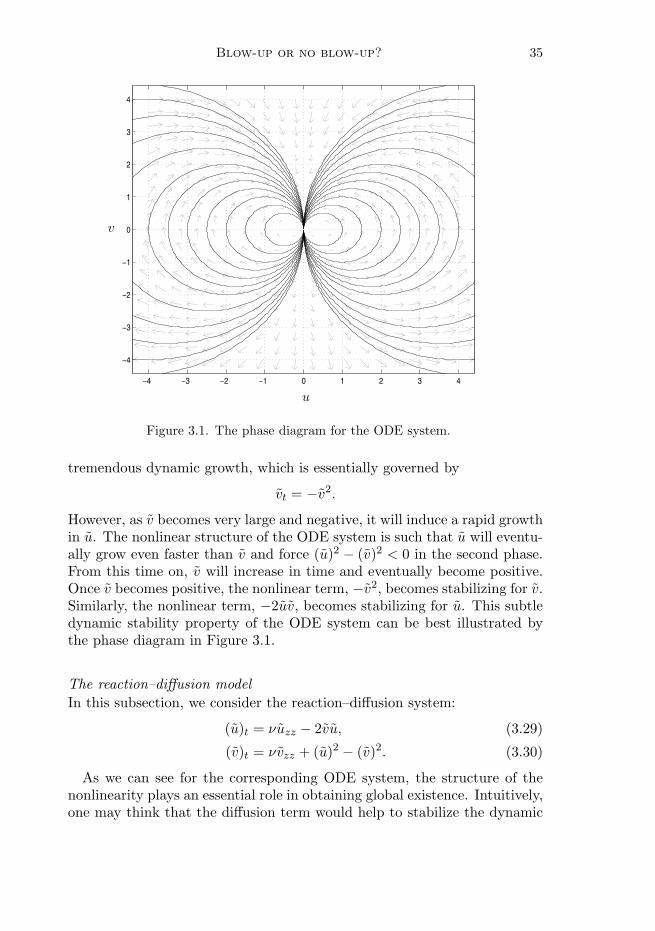
Blow-up or no blow-up? 35
−4 −3 −2 −1 0 1 2 3 4
−4
−3
−2
−1
0
1
2
3
4
v
u
Figure 3.1. The phase diagram for the ODE system.
tremendous dynamic growth, which is essentially governed by
vt = −v2.
However, as v becomes very large and negative, it will induce a rapid growthin u. The nonlinear structure of the ODE system is such that u will eventu-ally grow even faster than v and force (u)2 − (v)2 < 0 in the second phase.From this time on, v will increase in time and eventually become positive.Once v becomes positive, the nonlinear term, −v2, becomes stabilizing for v.Similarly, the nonlinear term, −2uv, becomes stabilizing for u. This subtledynamic stability property of the ODE system can be best illustrated bythe phase diagram in Figure 3.1.
The reaction–diffusion modelIn this subsection, we consider the reaction–diffusion system:
(u)t = νuzz − 2vu, (3.29)
(v)t = νvzz + (u)2 − (v)2. (3.30)
As we can see for the corresponding ODE system, the structure of thenonlinearity plays an essential role in obtaining global existence. Intuitively,one may think that the diffusion term would help to stabilize the dynamic
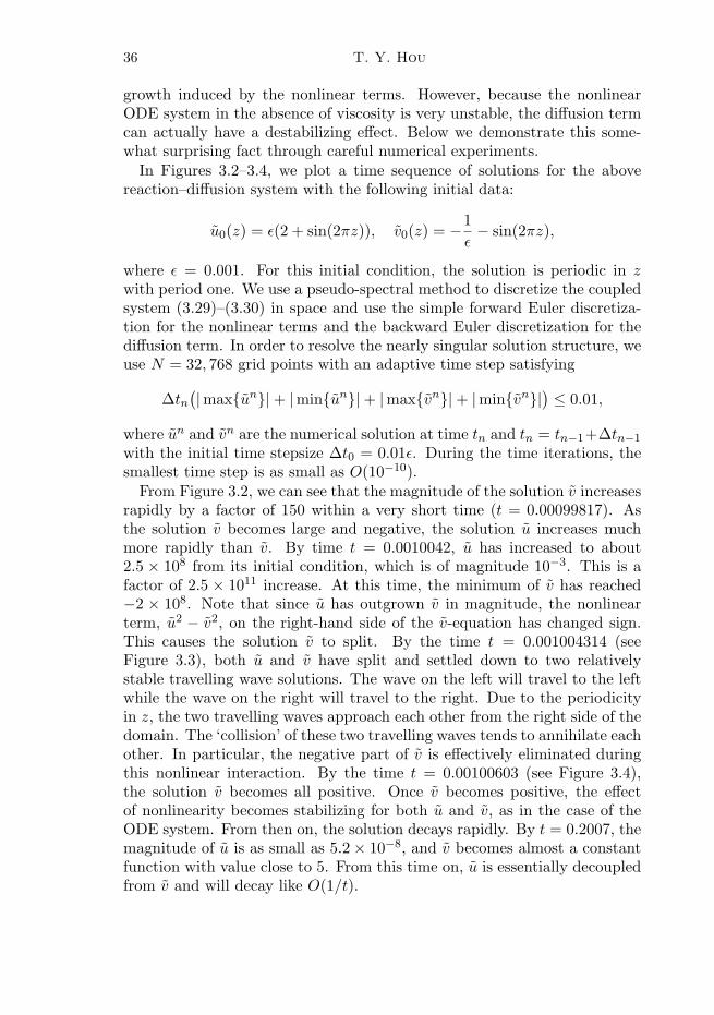
36 T. Y. Hou
growth induced by the nonlinear terms. However, because the nonlinearODE system in the absence of viscosity is very unstable, the diffusion termcan actually have a destabilizing effect. Below we demonstrate this some-what surprising fact through careful numerical experiments.
In Figures 3.2–3.4, we plot a time sequence of solutions for the abovereaction–diffusion system with the following initial data:
u0(z) = ε(2 + sin(2πz)), v0(z) = −1ε− sin(2πz),
where ε = 0.001. For this initial condition, the solution is periodic in zwith period one. We use a pseudo-spectral method to discretize the coupledsystem (3.29)–(3.30) in space and use the simple forward Euler discretiza-tion for the nonlinear terms and the backward Euler discretization for thediffusion term. In order to resolve the nearly singular solution structure, weuse N = 32, 768 grid points with an adaptive time step satisfying
∆tn(|maxun| + |minun| + |maxvn| + |minvn|) ≤ 0.01,
where un and vn are the numerical solution at time tn and tn = tn−1+∆tn−1
with the initial time stepsize ∆t0 = 0.01ε. During the time iterations, thesmallest time step is as small as O(10−10).
From Figure 3.2, we can see that the magnitude of the solution v increasesrapidly by a factor of 150 within a very short time (t = 0.00099817). Asthe solution v becomes large and negative, the solution u increases muchmore rapidly than v. By time t = 0.0010042, u has increased to about2.5 × 108 from its initial condition, which is of magnitude 10−3. This is afactor of 2.5 × 10¹¹ increase. At this time, the minimum of v has reached−2 × 10⁸. Note that since u has outgrown v in magnitude, the nonlinearterm, u2 − v2, on the right-hand side of the v-equation has changed sign.This causes the solution v to split. By the time t = 0.001004314 (seeFigure 3.3), both u and v have split and settled down to two relativelystable travelling wave solutions. The wave on the left will travel to the leftwhile the wave on the right will travel to the right. Due to the periodicityin z, the two travelling waves approach each other from the right side of thedomain. The ‘collision’ of these two travelling waves tends to annihilate eachother. In particular, the negative part of v is effectively eliminated duringthis nonlinear interaction. By the time t = 0.00100603 (see Figure 3.4),the solution v becomes all positive. Once v becomes positive, the effectof nonlinearity becomes stabilizing for both u and v, as in the case of theODE system. From then on, the solution decays rapidly. By t = 0.2007, themagnitude of u is as small as 5.2 × 10⁻⁸, and v becomes almost a constantfunction with value close to 5. From this time on, u is essentially decoupledfrom v and will decay like O(1/t).
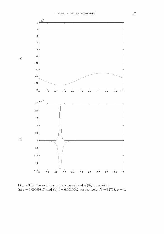
Blow-up or no blow-up? 37
(a)
0 0.1 0.2 0.3 0.4 0.5 0.6 0.7 0.8 0.9 1.0−18
−16
−14
−12
−10
−8
−6
−4
−2
0
2x 10
4
(b)
0 0.1 0.2 0.3 0.4 0.5 0.6 0.7 0.8 0.9 1.0−2.0
−1.5
−1.0
−0.5
0
0.5
1.0
1.5
2.0
2.5x 10
8
Figure 3.2. The solutions u (dark curve) and v (light curve) at(a) t = 0.00099817, and (b) t = 0.0010042, respectively; N = 32768, ν = 1.
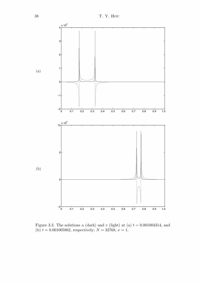
38 T. Y. Hou
(a)
0 0.1 0.2 0.3 0.4 0.5 0.6 0.7 0.8 0.9 1.0−2
−1
0
1
2
3
4x 10
8
(b)
0 0.1 0.2 0.3 0.4 0.5 0.6 0.7 0.8 0.9 1.0−5
0
5
10x 10
8
Figure 3.3. The solutions u (dark) and v (light) at (a) t = 0.001004314, and(b) t = 0.001005862, respectively; N = 32768, ν = 1.
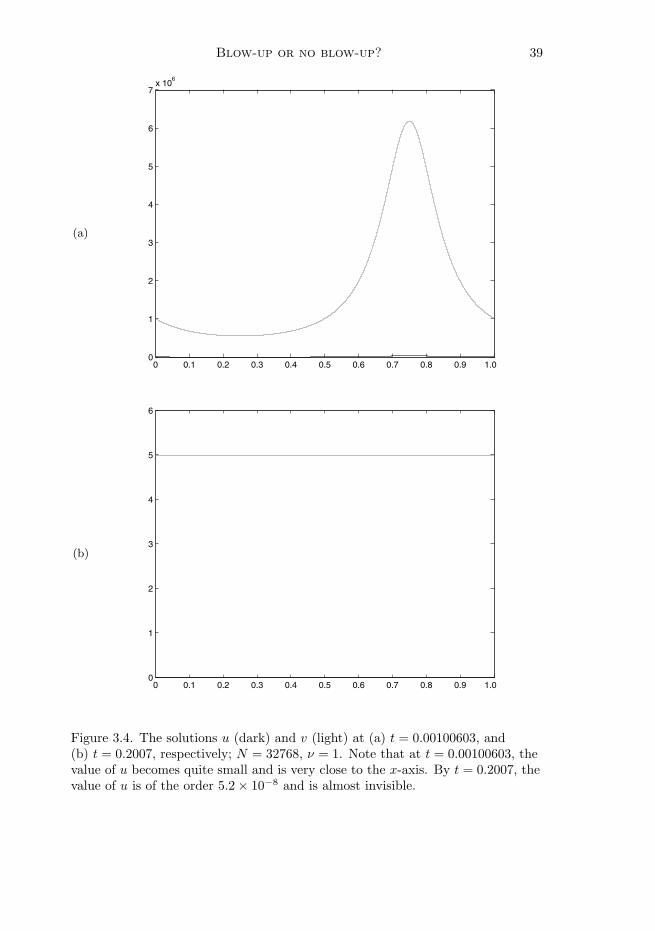
Blow-up or no blow-up? 39
(a)
0 0.1 0.2 0.3 0.4 0.5 0.6 0.7 0.8 0.9 1.00
1
2
3
4
5
6
7x 10
6
(b)
0 0.1 0.2 0.3 0.4 0.5 0.6 0.7 0.8 0.9 1.00
1
2
3
4
5
6
Figure 3.4. The solutions u (dark) and v (light) at (a) t = 0.00100603, and(b) t = 0.2007, respectively; N = 32768, ν = 1. Note that at t = 0.00100603, thevalue of u becomes quite small and is very close to the x-axis. By t = 0.2007, thevalue of u is of the order 5.2 × 10⁻⁸ and is almost invisible.
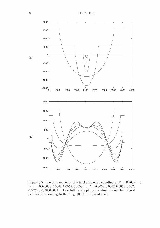
40 T. Y. Hou
(a)
0 500 1000 1500 2000 2500 3000 3500 4000 4500−2000
−1500
−1000
−500
0
500
1000
1500
2000
(b)
0 500 1000 1500 2000 2500 3000 3500 4000 4500−1500
−1000
−500
0
500
1000
1500
2000
Figure 3.5. The time sequence of v in the Eulerian coordinate, N = 4096, ν = 0.(a) t = 0, 0.0033, 0.0048, 0.0055, 0.0059, (b) t = 0.0059, 0.0062, 0.0066, 0.007,0.0074, 0.0078, 0.0081. The solutions are plotted against the number of gridpoints corresponding to the range [0, 1] in physical space.
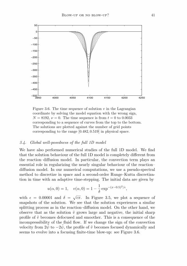
Blow-up or no blow-up? 41
3950 4000 4050 4100 4150 4200 4250−500
−450
−400
−350
−300
−250
−200
−150
−100
−50
0
50
Figure 3.6. The time sequence of solution v in the Lagrangiancoordinate by solving the model equation with the wrong sign,N = 8192, ν = 0. The time sequence is from t = 0 to 0.0033corresponding to a sequence of curves from the top to the bottom.The solutions are plotted against the number of grid pointscorresponding to the range [0.482, 0.519] in physical space.
3.4. Global well-posedness of the full 1D model
We have also performed numerical studies of the full 1D model. We findthat the solution behaviour of the full 1D model is completely different fromthe reaction–diffusion model. In particular, the convection term plays anessential role in regularizing the nearly singular behaviour of the reaction–diffusion model. In our numerical computations, we use a pseudo-spectralmethod to discretize in space and a second-order Runge–Kutta discretiza-tion in time with an adaptive time-stepping. The initial data are given by
u(α, 0) = 1, v(α, 0) = 1 − 1δ
exp−(x−0.5)2/ε,
with ε = 0.00001 and δ =√επ. In Figure 3.5, we plot a sequence of
snapshots of the solution. We see that the solution experiences a similarsplitting process as in the reaction–diffusion model. On the other hand, weobserve that as the solution v grows large and negative, the initial sharpprofile of v becomes defocused and smoother. This is a consequence of theincompressibility of the fluid flow. If we change the sign of the convectionvelocity from 2ψ to −2ψ, the profile of v becomes focused dynamically andseems to evolve into a focusing finite-time blow-up: see Figure 3.6.
42 T. Y. Hou
Based on our numerical studies, we become convinced that the solution ofthe full 1D model should be regular for all times. However, it is extremelydifficult, if not impossible, to prove the global regularity of the 1D modelby using an energy type of estimates. If we multiply the u-equation by u,and the v-equation by v, and integrate over z, we arrive at
12
ddt
∫ 1
0u2 dz = −3
∫ 1
0(u)2v dz − ν
∫ 1
0u2
z dz, (3.31)
12
ddt
∫ 1
0v2 dz =
∫ 1
0u2v dz − 3
∫ 1
0(v)3 dz − ν
∫ 1
0v2z dz. (3.32)
Even for this 1D model, the energy estimate shares the some essentialdifficulty as the 3D Navier–Stokes equations. It is not clear how to controlthe nonlinear vortex-stretching-like terms by the diffusion term. On theother hand, if we assume that
∫ T
0‖v‖L∞ dt <∞,
similar to the Beale–Kato–Majda non-blow-up condition for vorticity (Beale,Kato and Majda 1984), then one can easily show that there is no blow-upbefore t = T .
In order to obtain the global regularity of the 1D model, we need to use alocal estimate. The key is to obtain a pointwise estimate for a positive Lya-punov function. Convection is found to play an essential role in cancellingthe destabilizing vortex stretching terms. Using this pointwise estimate, wecan prove that if the initial conditions for u and v are in Cm with m ≥ 1,then the solution remains in Cm for all times.
Theorem 3.3. (Hou and Li 2008a) Assume that u(z, 0) and v(z, 0) arein Cm[0, 1] with m ≥ 1 and periodic with period 1. Then the solution (u, v)of the 1D model will be in Cm[0, 1] for all times and for ν ≥ 0.
Proof. The key is to obtain a pointwise estimate a priori for the positiveLyapunov function u2
z + v2z . Differentiating (3.20)–(3.21) with respect to z,
we get
(uz)t + 2ψ(uz)z − 2vuz = −2vuz − 2uvz + ν(uz)zz, (3.33)
(vz)t + 2ψ(vz)z − 2vvz = 2uuz − 2vvz + ν(vz)zz. (3.34)
Note that the convection term contributes to stability by cancelling one ofthe nonlinear terms on the right-hand side. This gives
(uz)t + 2ψ(uz)z = −2uvz + ν(uz)zz, (3.35)
(vz)t + 2ψ(vz)z = 2uuz + ν(vz)zz. (3.36)
Blow-up or no blow-up? 43
Multiplying (3.35) by 2uz and (3.36) by 2vz, we obtain
(u2z)t + 2ψ(u2
z)z = −4uuz vz + 2νuz(uz)zz, (3.37)
(v2z)t + 2ψ(v2
z)z = 4uuz vz + 2νvz(vz)zz. (3.38)
Now, we add (3.37) to (3.38). Surprisingly, the remaining nonlinear vortexstretching terms cancel each other exactly. We get
(u2
z + v2z
)t+ 2ψ
(u2
z + v2z
)z
= 2ν(uz(uz)zz + vz(vz)zz
). (3.39)
Further, we can rewrite equation (3.39) as follows:(u2
z + v2z
)t+ 2ψ
(u2
z + v2z
)z
= ν(u2
z + v2z
)zz
− 2ν[(uzz)2 + (vzz)2
]. (3.40)
Now it is easy to see that (u2z + v2
z) satisfies a maximum principle for allν ≥ 0:
‖u2z + v2
z‖L∞ ≤ ‖(u0)2z + (v0)2z‖L∞ .
It is worth emphasizing that the cancellation between the convection termand the vortex stretching term takes place at the inviscid level. Viscositydoes not play an essential role here. Since v has zero mean, the Poincareinequality implies that ‖v‖L∞ ≤ C0, with C0 defined by
C0 = ‖((u0)2z + (v0)2z) 1
2 ‖L∞ .
The boundedness of u follows from the bound on v, that is, ‖u(t)‖L∞ ≤‖u0‖L∞ exp(2C0t). The higher-order regularity follows from the standardestimates. This proves Theorem 3.3.
3.5. Construction of a family of 3D globally smooth solutions
We can use the solution from the 1D model to construct a family of glob-ally smooth solutions for the 3D axisymmetric Navier–Stokes equationswith large initial data of finite energy. We remark that a special fea-ture of this family of globally smooth solutions is that the solution canpotentially develop very large dynamic growth and it violates the small-ness condition required by classical global existence results (Constantin andFoias 1988, Temam 2001).
Theorem 3.4. (Hou and Li 2008a) Let φ(r) be a smooth cut-off func-tion and u1, ω1 and ψ1 be the solution of the 1D model. Define
uθ(r, z, t) = ru1(z, t)φ(r) + u(r, z, t),
ωθ(r, z, t) = rω1(z, t)φ(r) + ω(r, z, t),
ψθ(r, z, t) = rψ1(z, t)φ(r) + ψ(r, z, t).
44 T. Y. Hou
Then there exists a family of globally smooth functions u, ω and ψ suchthat uθ, ωθ and ψθ are globally smooth solutions of the 3D Navier–Stokesequations with finite energy.
4. Stabilizing effect of convection for 3D Navier–Stokes
Hou and Lei (2009b) studied the stabilizing effect of the convection termin the 3D incompressible Euler or Navier–Stokes equations using a new3D model. This model was derived from the reformulated Navier–Stokesequations. It shares many properties with the 3D Euler or Navier–Stokesequations. First of all, it has the same nonlinear vortex stretching term.Secondly, it has the same type of a priori energy identity. Thirdly, al-most all the existing non-blow-up criteria for the 3D Euler or Navier–Stokesequations are also valid for our model. A 3D model that satisfies all theseproperties seems hard to find in general. But in terms of the equations forthe new variables, u1, ω1, and ψ1, we obtain our 3D model equations bysimply dropping the convective term from the reformulated Navier–Stokesequations (3.16):
∂tu1 = ν
(
∂2r +
3r∂r + ∂2
z
)
u1 + 2u1ψ1z, (4.1a)
∂tω1 = ν
(
∂2r +
3r∂r + ∂2
z
)
ω1 + (u21)z, (4.1b)
−(
∂2r +
3r∂r + ∂2
z
)
ψ1 = ω1. (4.1c)
Note that (4.1) is already a closed system. The main difference between our3D model and the Navier–Stokes equations is that we neglect the convectionterm in our model. If we add the convection term back to our 3D model,we will recover the Navier–Stokes equations.
Below we will summarize some important properties of the model equa-tions (4.1).
4.1. Properties of the 3D model
This 3D model shares many important properties with the axisymmetricNavier–Stokes equations. First of all, one can define an incompressiblevelocity field for the 3D model,
u(t,x) = ur(t, r, z)er + uθ(t, r, z)eθ + uz(t, r, z)ez, (4.2)
uθ = ru1, ur = −rψ1z, uz = 2ψ1 + rψ1r, (4.3)
where x = (x, y, z), r =√x2 + y2. It is easy to check that
∇ · u = ∂rur + ∂zu
z +ur
r= 0, (4.4)
Blow-up or no blow-up? 45
which is the same as the original Navier–Stokes equations.Furthermore, Hou and Lei (2009b) proved the following energy identity
for the 3D model.
Theorem 4.1. (Energy identity (Hou and Lei 2009b)) The strong so-lution of (4.1) satisfies
12
ddt
∫ (|u1|2 + 2|Dψ1|2)r3 dr dz + ν
∫ (|Du1|2 + 2|D2ψ1|2)r3 dr dz = 0,
(4.5)
Here D is the first-order derivative operator defined in R5.
This energy identity is equivalent to that of the Navier–Stokes equations,which has the form
12
ddt
∫ (|u1|2 + |Dψ1|2)r3 dr dz + ν
∫ (|Du1|2 + |D2ψ1|2)r3 dr dz = 0.
(4.6)
Another result obtained by Hou and Lei is a non-blow-up criterion of the3D model equations (4.1), which is an analogue of the Beale–Kato–Majda(BKM) result for the 3D Euler and Navier–Stokes equations. For the 3DEuler and Navier–Stokes equations, the BKM non-blow-up criterion statesthat the solution u blows up at time T <∞ if and only if the accumulation ofvorticity
∫ T0 ‖∇x×u‖L∞(R3) dt is infinite (Beale, Kato and Majda 1984). The
BKM non-blow-up criterion was later improved by Kozono and Taniuchi(2000), who proved that the ‖ · ‖L∞-norm can be replaced by the normin the BMO space. This generalization is interesting because some crucialSobolev embedding theorems can be applied to the BMO space, but not tothe L∞-space. A non-blow-up result formulated in terms of the BMO spacehas a broader range of applications.
Theorem 4.2. (Anon-blow-up criterion ofBeale–Kato–Majda type(Hou and Lei 2009b)) A smooth solution (u1, ω1, ψ1) of the model (4.1)for 0 ≤ t < T blows up at time t = T if and only if
∫ T
0‖∇ × u‖BMO(R3) dt = ∞, (4.7)
where u is defined in (4.2)–(4.3).
There have been many results on the global regularity of the solutionsof the 3D Navier–Stokes equations under some additional conditions im-posed on the solution. In particular, the papers of Prodi (1959) and Serrin(1963) gave the following non-blow-up criterion for the solution of the 3DNavier–Stokes equations: Any Leray–Hopf solution u to the 3D Navier–Stokes equations on [0, T ] is smooth on [0, T ] if ‖u‖Lq
t Lpx([0,T ]×R3) < ∞ for
46 T. Y. Hou
some p, q satisfying (3/p)+(2/q) ≤ 1, 3 < p ≤ ∞. A local version was laterestablished by Serrin (1962) for (3/p) + (2/q) < 1 and by Struwe (1988)for (3/p) + (2/q) = 1. The highly non-trivial end-point case of p = 3 wasrecently established by Iskauriaza, Seregin and Sverak (2003).
To demonstrate the similarity between the 3D model equations (4.1) andthe axisymmetric Navier–Stokes equations, Hou and Lei proved a non-blow-up criterion of the Prodi–Serrin type for their model.
Theorem 4.3. (A non-blow-up criterion of Prodi–Serrin type (Houand Lei 2009b)) A weak solution (u1, ω1, ψ1) of the model (4.1) is smoothon [0, T ] × R3 provided that
‖uθ‖Lqt Lp
x([0,T ]×R3) <∞ (4.8)
for some p, q satisfying 3p + 2
q ≤ 1 with 3 < p ≤ ∞ and 2 ≤ q <∞.
Finally, Hou and Lei (2009a) studied the local behaviour of the solutionsto the 3D model equations and established an analogue of the Caffarelli–Kohn–Nirenberg partial regularity theory (Caffarelli et al. 1982) for theirmodel. They proved that for any suitable weak solution of the 3D modelin an open set in space-time, the one-dimensional Hausdorff measure of theassociated singular set is zero. The proof of this partial regularity resultis similar in spirit to that of Lin (1998), but there are some new technicaldifficulties associated with the 3D model. One of the difficulties is in han-dling the singularity induced by the cylindrical coordinates. This makes itdifficult to analyse the partial regularity of the 3D model in R × R3. Toovercome this difficulty, they performed their partial regularity analysis inR × R5. By working in R5, they avoided the difficulty associated with thecoordinate singularity.
Another difficulty in obtaining our partial regularity result is that we donot have an evolution equation for the entire velocity field. We need toreformulate the model in terms of a new vector variable. This new variablecan be considered as a ‘generalized velocity field’ in R5. We remark thatthe partial regularity theory for Navier–Stokes equations in R5 is still opendue to the lack of certain compactness. When formulating the 3D model inR × R5, they found a 3D structure which has the same scaling as that ofthe 3D Navier–Stokes equations. This is why the partial regularity analysiscan be carried out for the 3D model in R × R5 using a strategy similar tothat of Lin (1998).
Theorem 4.4. (An analogue of Caffarelli–Kohn–Nirenberg partialregularity result (Hou and Lei 2009a)) For any suitable weak solutionof the 3D model equations (4.1) on an open set in space-time, the one-dimensional Hausdorff measure of the associated singular set is zero.

Blow-up or no blow-up? 47
4.2. Potential singularity formation of the 3D model
Despite the striking similarity at the theoretical level between the 3D modeland the Navier–Stokes equations, the former displays a completely differentbehaviour from the full Navier–Stokes equations. In the next subsection,we will present numerical evidence which seems to support that the modelmay develop a potential finite-time singularity from smooth initial data withfinite energy. Before we do that, we would like to gain some understanding atthe theoretical level why the 3D model may develop a finite-time singularity.For this purpose, we consider the inviscid model by setting ν = 0 in (4.1):
∂tu1 = 2u1ψ1z, (4.9a)
∂tω1 = (u21)z, (4.9b)
−(
∂2r +
3r∂r + ∂2
z
)
ψ1 = ω1. (4.9c)
If we let v = log(u21), then we can further reduce the 3D model to the
following non-local nonlinear wave equation:
vtt = 4((−∆5)−1ev
)zz, (4.10)
where −∆5 = −(∂2
r + 3r∂r +∂2
z
), and
∫evr3 dr dz ≤ C0. Note that (−∆5)−1
is a positive operator. If we were to omit (−∆5)−1 from (4.10), we wouldobtain a 1D nonlinear wave equation, vtt = 4(ev)zz, or
vtt = 4evvzz + 4ev(vz)2, (4.11)
which we expect to develop a finite-time singularity.
4.3. Special blow-up solutions of the 3D model
We can construct a special class of blow-up solutions by letting u1 = zu(r, t),ω1 = zω(r, t), and ψ1 = zψ(r, t). Then it is easy to derive the followingsystem for u(r, t), ω(r, t), and ψ(r, t):
∂tu = 2ψu+ ν(∂2r +
3r∂r)u, (4.12a)
∂tω = 2u2 + ν(∂2r +
3r∂r)ω, (4.12b)
−(
∂2r +
3r∂r
)
ψ = ω. (4.12c)
Note that the nonlinear terms become local and quadratic. It is easy to showthat if the initial data are positive, then the solution of (4.12) will remainpositive for all times. Using this property, we can prove that the abovesystem has finite-time blow-up solutions. However, such singular solutionshave infinite energy unless we introduce a cut-off along the z-direction.
48 T. Y. Hou
We remark that Constantin (1986) has constructed a family of finite-timeblow-up solutions to the distorted Euler equations:
(∇u)t + (∇u)2 + ∇∇p = 0, (4.13)
where −∆p = Tr((∇u)2). We note that u is no longer divergence-free (infact, there is no evolution equation for u), and the model does not conserveenergy. Moreover, the blow-up solution has infinite energy.
4.4. Numerical evidence for a potential finite-time singularity
In this subsection, we present numerical evidence which seems to supportthat the model may develop a potential finite-time singularity from smoothinitial data with finite energy. By exploiting the axisymmetric geometryof the problem, we obtain a very efficient adaptive solver with an optimalcomplexity which provides effective local resolutions of order 40963. Withthis level of resolution, we obtain an excellent fit for the asymptotic blow-up rate of maximum axial vorticity. If we denote by ωz the axial vorticitycomponent along the z-direction, we find that ‖ωz‖∞(t) ≈ C(T − t)−1 andthe potential singularity approaches the symmetry axis (the z-axis) as t→T . Moreover, our study seems to suggest that the potential singularity islocally self-similar and isotropic.
The initial condition considered in our numerical computations is given by
u1(z, r, 0) = (1 + sin(4πz))(r2 − 1)20(r2 − 1.2)30, (4.14)ψ1(z, r, 0) = 0, (4.15)ω1(z, r, 0) = 0. (4.16)
A second-order finite-difference discretization is used in space, and the clas-sical fourth-order Runge–Kutta method is used to discretize in time. Sincewe expect that the potential singularity will appear along the symmetryaxis at r = 0, we use the following coordinate transformation along the r-direction to achieve the adaptivity by clustering the grid points near r = 0:
r = f(α) ≡ α− 0.9 sin(πα)/π. (4.17)
With this change of variables, we can achieve an effective resolution up to40963 for the corresponding 3D problem.
We now present numerical results which show that the solution of theviscous model becomes nearly singular. We choose the viscous coefficient tobe ν = 0.001 and perform a series of resolution studies using the adaptivemethod. We have used both uniform mesh and adaptive mesh with Nz
ranging from 256 to 4096. Below we present the computational resultsobtained by using the adaptive mesh with the highest resolution Nz = 4096,Nr = 400, and ∆t = 2.5× 10⁻⁷. We will also perform a resolution study todemonstrate that our computations are well resolved.
Blow-up or no blow-up? 49
From our analytical study of the 3D model, it follows by using a standardenergy estimate that if u1 is bounded, then the solution of the viscous 3Dmodel cannot blow up in a finite time. Thus it is sufficient to monitor thegrowth of ‖u1‖∞ in time. We will present numerical evidence which seemsto support that u1 may develop a potential finite-time singularity for theinitial condition we consider. The nature of this potential singularity andthe mechanism for generating this potential singularity will be analysed ina later subsection.
In Figure 4.1, we plot the maximum of u1 in time over the time interval[0, 0.021] using the adaptive mesh method with Nz = 4096 and Nr = 400.The time step is chosen to be ∆t = 2.5×10⁻⁷. We can see that ‖u1‖∞ expe-riences a very rapid growth in time after t = 0.02. In Figure 4.1(b), we alsoplot log(log(‖u1‖∞)) as a function of time. We can see clearly that ‖u1‖∞grows much more rapidly than double exponential in time, which impliesthat the solution of our model may develop a finite-time singularity. We willpresent more careful analysis of this potentially singular behaviour later.
In Figures 4.2–4.3, we show a sequence of contour plots for u1 fromt = 0.014 to t = 0.021. At early times, we observe that the solution formstwo large focusing centres of u1 which approach each other. As this occurs,these rather localized regions are squeezed and form a thin layer parallelto the r-axis and with large gradients along the z-direction. As these re-gions approach each other and develop a thin layer parallel to the r-axis,the solution becomes locally z-dominant near the region where u1 achievesits maximum. In this region, the 3D model can be approximated to theleading order by the corresponding 1D model along the z-direction. Houand Lei (2009b) proved that the solution of the 1D model cannot blow up.The solution survives this potential blow-up scenario. After t = 0.0172,the maximum of u1 starts to decrease. The two focusing centres moveaway from each other and their supports become more isotropic. As timeincreases, we observe that there is a strong nonlinear interaction betweenu1 and (ψ1)z, which is induced by the overlap between the support of max-imum of u1 and the support of maximum of (ψ1)z. By the support ofmaximum of u1, we mean the region in which u1 is comparable to its max-imum. The strong alignment between u1 and (ψ1)z near the support ofmaximum of u1 leads to a rapid growth of the solution which may becomesingular in a finite time.
Another important observation is that as time increases, the position atwhich u1 achieves its maximum also moves towards the symmetry axis. Thissuggests that the potential singularity will be along the symmetry axis atthe singularity time. We note that limr→0+ u1 = 0.5 limr→0+ ω
z. Thus, theblow-up of u1 characterizes the blow-up of the axial vorticity, ωz.
Next, we perform a detailed study for the 3D model and push our com-putations very close to the potential singularity time. We use a sequence of
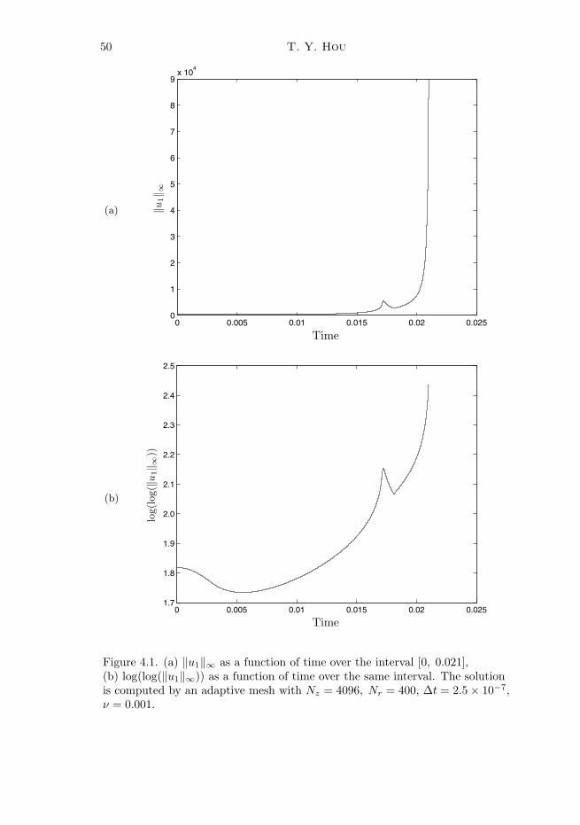
50 T. Y. Hou
(a)
0 0.005 0.01 0.015 0.02 0.0250
1
2
3
4
5
6
7
8
9x 10
4
‖u1‖ ∞
Time
(b)
0 0.005 0.01 0.015 0.02 0.0251.7
1.8
1.9
2.0
2.1
2.2
2.3
2.4
2.5
log(
log(‖u
1‖ ∞
))
Time
Figure 4.1. (a) ‖u1‖∞ as a function of time over the interval [0, 0.021],(b) log(log(‖u1‖∞)) as a function of time over the same interval. The solutionis computed by an adaptive mesh with Nz = 4096, Nr = 400, ∆t = 2.5 × 10⁻⁷,ν = 0.001.
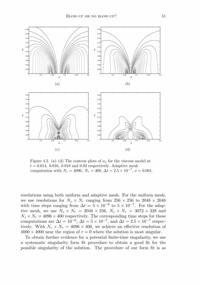
Blow-up or no blow-up? 51
0.3 0.35 0.4 0.45 0.50
0.02
0.04
0.06
0.08
0.10
0.12
0.14
0.16
0.18
0.20
r
z
(a)
0.3 0.35 0.4 0.45 0.50
0.02
0.04
0.06
0.08
0.10
0.12
0.14
0.16
0.18
0.20
r
z
(b)
0.3 0.35 0.4 0.45 0.50
0.02
0.04
0.06
0.08
0.10
0.12
0.14
0.16
0.18
0.20
r
z
(c)
0.3 0.35 0.4 0.45 0.50
0.02
0.04
0.06
0.08
0.10
0.12
0.14
0.16
0.18
0.20
r
z
(d)
Figure 4.2. (a)–(d) The contour plots of u1 for the viscous model att = 0.014, 0.016, 0.018 and 0.02 respectively. Adaptive meshcomputation with Nz = 4096, Nr = 400, ∆t = 2.5 × 10⁻⁷, ν = 0.001.
resolutions using both uniform and adaptive mesh. For the uniform mesh,we use resolutions for Nz × Nr ranging from 256 × 256 to 2048 × 2048with time steps ranging from ∆t = 5 × 10⁻⁶ to 5 × 10⁻⁷. For the adap-tive mesh, we use Nz × Nr = 2048 × 256, Nz × Nr = 3072 × 328 andNz ×Nr = 4096× 400 respectively. The corresponding time steps for thesecomputations are ∆t = 10−6, ∆t = 5 × 10⁻⁷, and ∆t = 2.5 × 10⁻⁷ respec-tively. With Nz × Nr = 4096 × 400, we achieve an effective resolution of4000 × 4000 near the region of r = 0 where the solution is most singular.
To obtain further evidence for a potential finite-time singularity, we usea systematic singularity form fit procedure to obtain a good fit for thepossible singularity of the solution. The procedure of our form fit is as
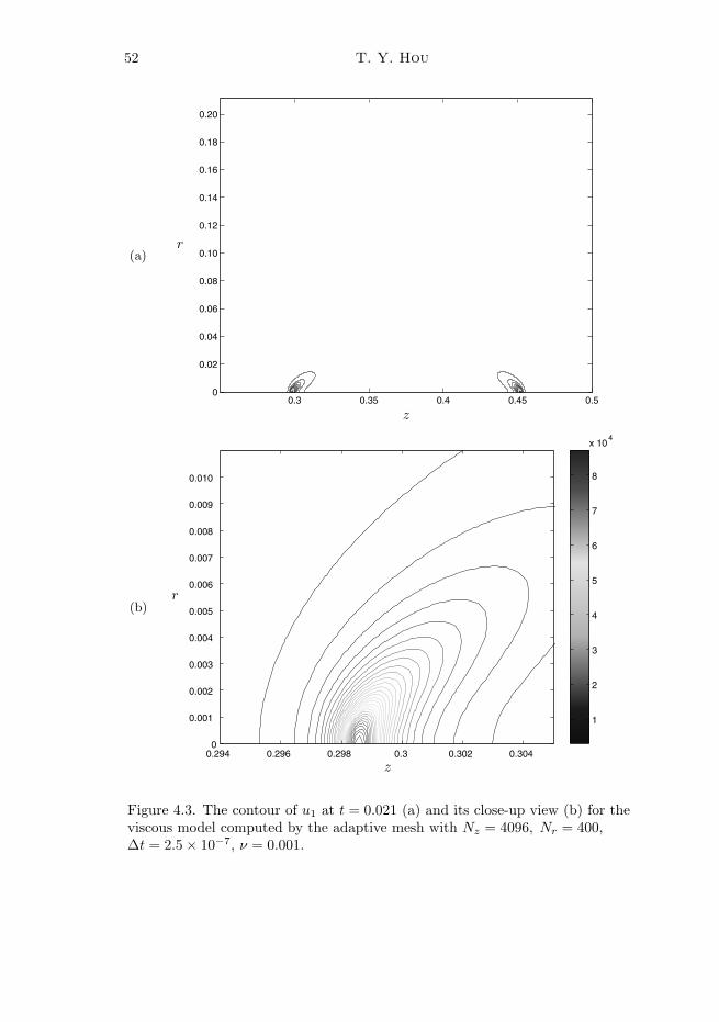
52 T. Y. Hou
(a)
0.3 0.35 0.4 0.45 0.50
0.02
0.04
0.06
0.08
0.10
0.12
0.14
0.16
0.18
0.20
r
z
(b)
0.294 0.296 0.298 0.3 0.302 0.3040
0.001
0.002
0.003
0.004
0.005
0.006
0.007
0.008
0.009
0.010
1
2
3
4
5
6
7
8
x 104
r
z
Figure 4.3. The contour of u1 at t = 0.021 (a) and its close-up view (b) for theviscous model computed by the adaptive mesh with Nz = 4096, Nr = 400,∆t = 2.5 × 10⁻⁷, ν = 0.001.
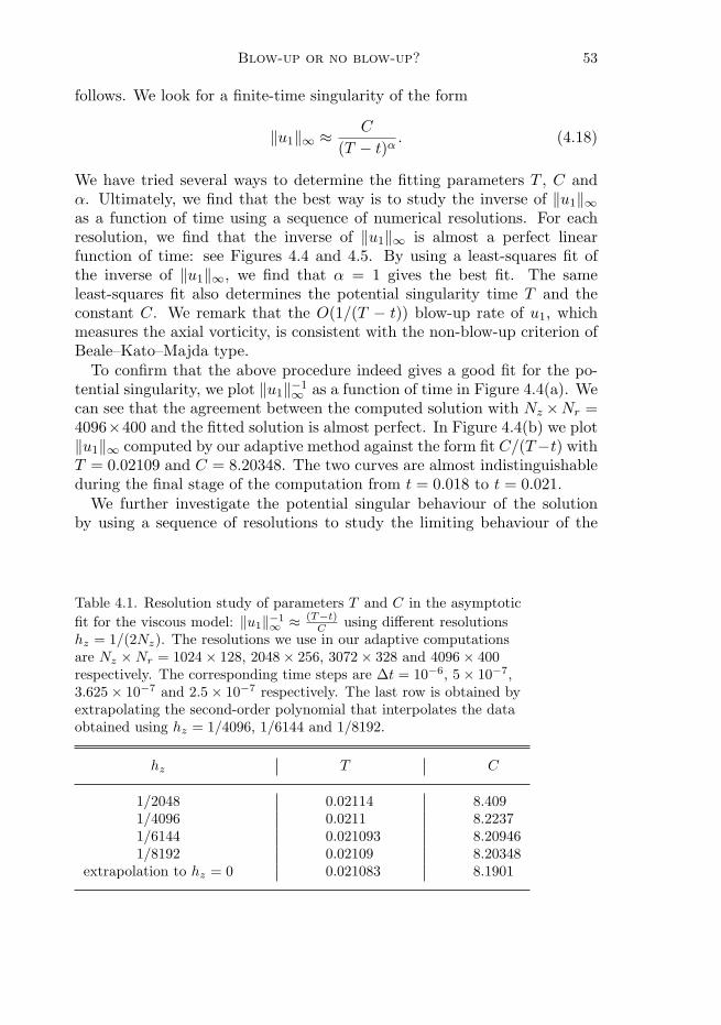
Blow-up or no blow-up? 53
follows. We look for a finite-time singularity of the form
‖u1‖∞ ≈ C
(T − t)α. (4.18)
We have tried several ways to determine the fitting parameters T , C andα. Ultimately, we find that the best way is to study the inverse of ‖u1‖∞as a function of time using a sequence of numerical resolutions. For eachresolution, we find that the inverse of ‖u1‖∞ is almost a perfect linearfunction of time: see Figures 4.4 and 4.5. By using a least-squares fit ofthe inverse of ‖u1‖∞, we find that α = 1 gives the best fit. The sameleast-squares fit also determines the potential singularity time T and theconstant C. We remark that the O(1/(T − t)) blow-up rate of u1, whichmeasures the axial vorticity, is consistent with the non-blow-up criterion ofBeale–Kato–Majda type.
To confirm that the above procedure indeed gives a good fit for the po-tential singularity, we plot ‖u1‖−1∞ as a function of time in Figure 4.4(a). Wecan see that the agreement between the computed solution with Nz ×Nr =4096×400 and the fitted solution is almost perfect. In Figure 4.4(b) we plot‖u1‖∞ computed by our adaptive method against the form fit C/(T−t) withT = 0.02109 and C = 8.20348. The two curves are almost indistinguishableduring the final stage of the computation from t = 0.018 to t = 0.021.
We further investigate the potential singular behaviour of the solutionby using a sequence of resolutions to study the limiting behaviour of the
Table 4.1. Resolution study of parameters T and C in the asymptoticfit for the viscous model: ‖u1‖−1
∞ ≈ (T−t)C using different resolutions
hz = 1/(2Nz). The resolutions we use in our adaptive computationsare Nz ×Nr = 1024 × 128, 2048 × 256, 3072 × 328 and 4096 × 400respectively. The corresponding time steps are ∆t = 10−6, 5 × 10−7,3.625 × 10−7 and 2.5 × 10⁻⁷ respectively. The last row is obtained byextrapolating the second-order polynomial that interpolates the dataobtained using hz = 1/4096, 1/6144 and 1/8192.
hz T C
1/2048 0.02114 8.4091/4096 0.0211 8.22371/6144 0.021093 8.209461/8192 0.02109 8.20348
extrapolation to hz = 0 0.021083 8.1901
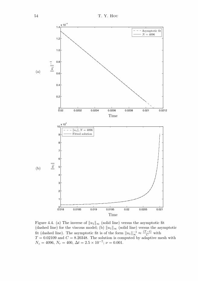
54 T. Y. Hou
(a)
0.02 0.0202 0.0204 0.0206 0.0208 0.021 0.02120
0.2
0.4
0.6
0.8
1.0
1.2
1.4x 10
−4
Time
‖u1‖−
1
Asymptotic fitN = 4096
(b)
0.018 0.0185 0.019 0.0195 0.02 0.0205 0.0210
1
2
3
4
5
6
7
8
9
10x 10
4
Time
‖u1‖
‖u1‖, N = 4096Fitted solution
Figure 4.4. (a) The inverse of ‖u1‖∞ (solid line) versus the asymptotic fit(dashed line) for the viscous model; (b) ‖u1‖∞ (solid line) versus the asymptoticfit (dashed line). The asymptotic fit is of the form ‖u1‖−1
∞ ≈ (T−t)C with
T = 0.02109 and C = 8.20348. The solution is computed by adaptive mesh withNz = 4096, Nr = 400, ∆t = 2.5 × 10⁻⁷; ν = 0.001.
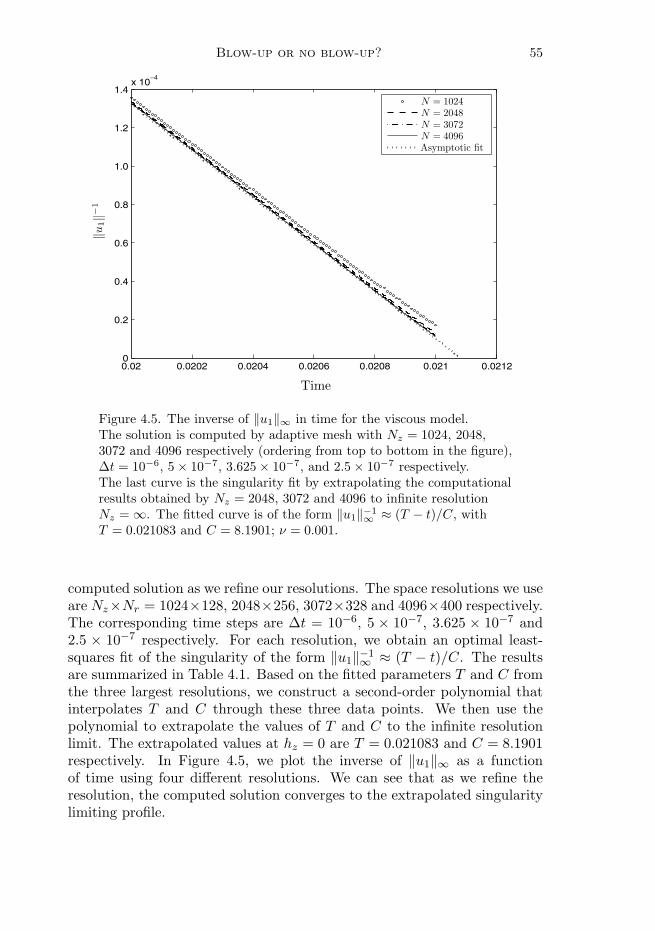
Blow-up or no blow-up? 55
0.02 0.0202 0.0204 0.0206 0.0208 0.021 0.02120
0.2
0.4
0.6
0.8
1.0
1.2
1.4x 10
−4
Time
N = 1024N = 2048N = 3072N = 4096Asymptotic fit
‖u1‖−
1
Figure 4.5. The inverse of ‖u1‖∞ in time for the viscous model.The solution is computed by adaptive mesh with Nz = 1024, 2048,3072 and 4096 respectively (ordering from top to bottom in the figure),∆t = 10−6, 5 × 10⁻⁷, 3.625 × 10⁻⁷, and 2.5 × 10⁻⁷ respectively.The last curve is the singularity fit by extrapolating the computationalresults obtained by Nz = 2048, 3072 and 4096 to infinite resolutionNz = ∞. The fitted curve is of the form ‖u1‖−1
∞ ≈ (T − t)/C, withT = 0.021083 and C = 8.1901; ν = 0.001.
computed solution as we refine our resolutions. The space resolutions we useare Nz×Nr = 1024×128, 2048×256, 3072×328 and 4096×400 respectively.The corresponding time steps are ∆t = 10−6, 5 × 10⁻⁷, 3.625 × 10⁻⁷ and2.5 × 10−7 respectively. For each resolution, we obtain an optimal least-squares fit of the singularity of the form ‖u1‖−1∞ ≈ (T − t)/C. The resultsare summarized in Table 4.1. Based on the fitted parameters T and C fromthe three largest resolutions, we construct a second-order polynomial thatinterpolates T and C through these three data points. We then use thepolynomial to extrapolate the values of T and C to the infinite resolutionlimit. The extrapolated values at hz = 0 are T = 0.021083 and C = 8.1901respectively. In Figure 4.5, we plot the inverse of ‖u1‖∞ as a functionof time using four different resolutions. We can see that as we refine theresolution, the computed solution converges to the extrapolated singularitylimiting profile.
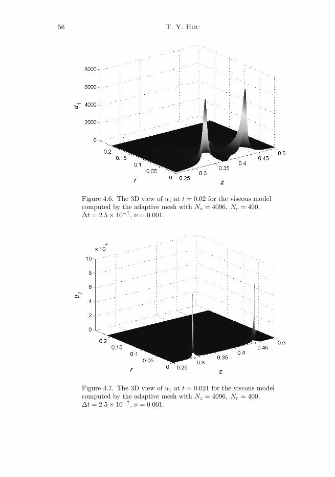
56 T. Y. Hou
Figure 4.6. The 3D view of u1 at t = 0.02 for the viscous modelcomputed by the adaptive mesh with Nz = 4096, Nr = 400,∆t = 2.5 × 10⁻⁷, ν = 0.001.
Figure 4.7. The 3D view of u1 at t = 0.021 for the viscous modelcomputed by the adaptive mesh with Nz = 4096, Nr = 400,∆t = 2.5 × 10⁻⁷, ν = 0.001.
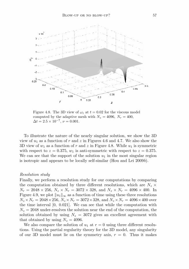
Blow-up or no blow-up? 57
Figure 4.8. The 3D view of ω1 at t = 0.02 for the viscous modelcomputed by the adaptive mesh with Nz = 4096, Nr = 400,∆t = 2.5 × 10⁻⁷, ν = 0.001.
To illustrate the nature of the nearly singular solution, we show the 3Dview of u1 as a function of r and z in Figures 4.6 and 4.7. We also show the3D view of w1 as a function of r and z in Figure 4.8. While u1 is symmetricwith respect to z = 0.375, w1 is anti-symmetric with respect to z = 0.375.We can see that the support of the solution u1 in the most singular regionis isotropic and appears to be locally self-similar (Hou and Lei 2009b).
Resolution studyFinally, we perform a resolution study for our computations by comparingthe computation obtained by three different resolutions, which are Nz ×Nr = 2048 × 256, Nz × Nr = 3072 × 328, and Nz × Nr = 4096 × 400. InFigure 4.9, we plot ‖u1‖∞ as a function of time using these three resolutionsNz×Nr = 2048×256, Nz×Nr = 3072×328, and Nz×Nr = 4096×400 overthe time interval [0, 0.021]. We can see that while the computation withNz = 2048 under-resolves the solution near the end of the computation, thesolution obtained by using Nz = 3072 gives an excellent agreement withthat obtained by using Nz = 4096.
We also compare the solution of u1 at r = 0 using three different resolu-tions. Using the partial regularity theory for the 3D model, any singularityof our 3D model must lie on the symmetry axis, r = 0. Thus it makes
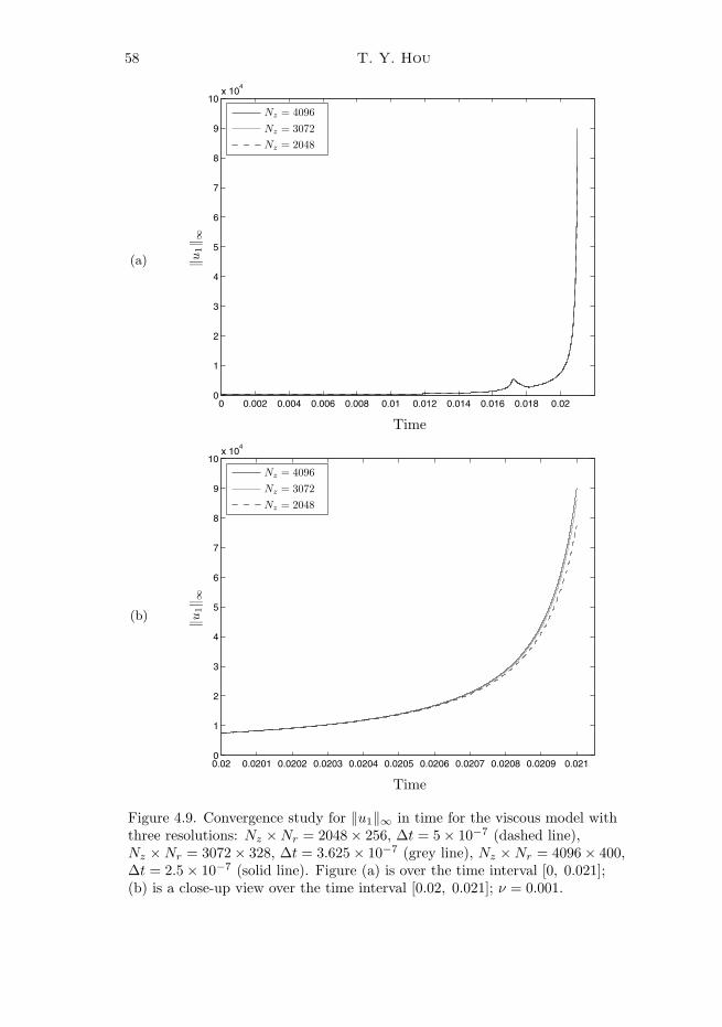
58 T. Y. Hou
(a)
0 0.002 0.004 0.006 0.008 0.01 0.012 0.014 0.016 0.018 0.020
1
2
3
4
5
6
7
8
9
10x 10
4
‖u1‖ ∞
Time
Nz = 4096Nz = 3072Nz = 2048
(b)
0.02 0.0201 0.0202 0.0203 0.0204 0.0205 0.0206 0.0207 0.0208 0.0209 0.0210
1
2
3
4
5
6
7
8
9
10x 10
4
‖u1‖ ∞
Time
Nz = 4096Nz = 3072Nz = 2048
Figure 4.9. Convergence study for ‖u1‖∞ in time for the viscous model withthree resolutions: Nz ×Nr = 2048 × 256, ∆t = 5 × 10⁻⁷ (dashed line),Nz ×Nr = 3072 × 328, ∆t = 3.625 × 10⁻⁷ (grey line), Nz ×Nr = 4096 × 400,∆t = 2.5 × 10⁻⁷ (solid line). Figure (a) is over the time interval [0, 0.021];(b) is a close-up view over the time interval [0.02, 0.021]; ν = 0.001.
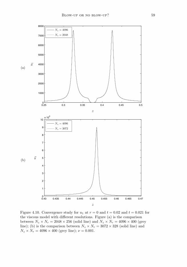
Blow-up or no blow-up? 59
(a)
0.25 0.3 0.35 0.4 0.45 0.50
1000
2000
3000
4000
5000
6000
7000
8000
u1
z
Nz = 4096
Nz = 2048
(b)
0.43 0.435 0.44 0.445 0.45 0.455 0.46 0.465 0.470
1
2
3
4
5
6
7
8
9
10x 10
4
u1
z
Nz = 4096
Nz = 3072
Figure 4.10. Convergence study for u1 at r = 0 and t = 0.02 and t = 0.021 forthe viscous model with different resolutions. Figure (a) is the comparisonbetween Nz ×Nr = 2048 × 256 (solid line) and Nz ×Nr = 4096 × 400 (greyline); (b) is the comparison between Nz ×Nr = 3072 × 328 (solid line) andNz ×Nr = 4096 × 400 (grey line); ν = 0.001.
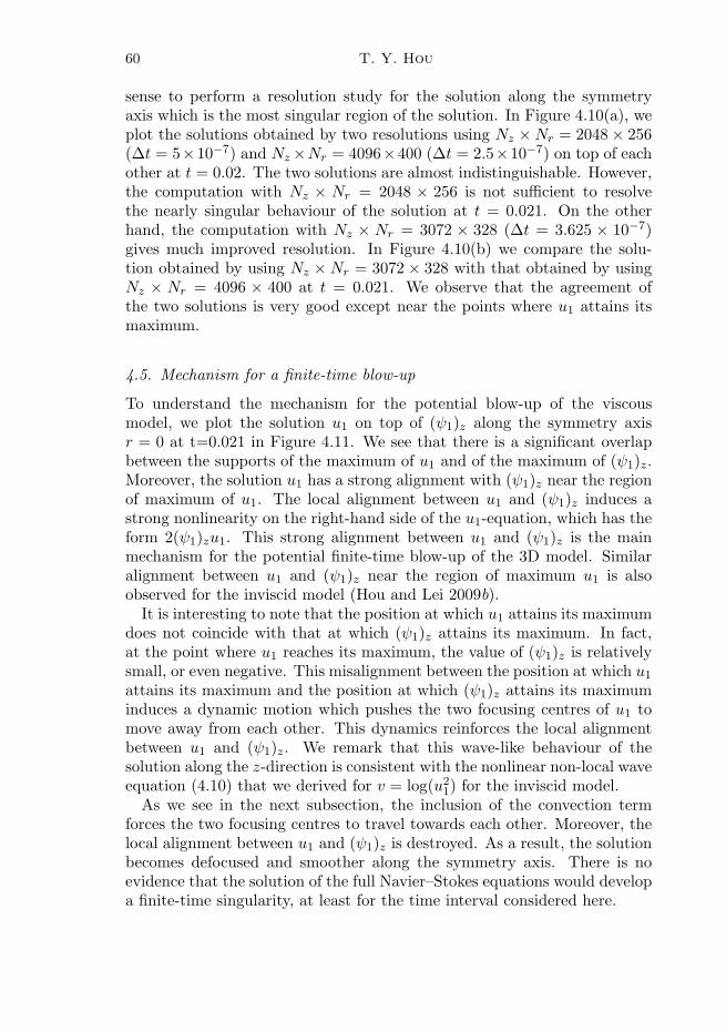
60 T. Y. Hou
sense to perform a resolution study for the solution along the symmetryaxis which is the most singular region of the solution. In Figure 4.10(a), weplot the solutions obtained by two resolutions using Nz ×Nr = 2048 × 256(∆t = 5×10⁻⁷) and Nz ×Nr = 4096×400 (∆t = 2.5×10⁻⁷) on top of eachother at t = 0.02. The two solutions are almost indistinguishable. However,the computation with Nz × Nr = 2048 × 256 is not sufficient to resolvethe nearly singular behaviour of the solution at t = 0.021. On the otherhand, the computation with Nz × Nr = 3072 × 328 (∆t = 3.625 × 10⁻⁷)gives much improved resolution. In Figure 4.10(b) we compare the solu-tion obtained by using Nz ×Nr = 3072 × 328 with that obtained by usingNz × Nr = 4096 × 400 at t = 0.021. We observe that the agreement ofthe two solutions is very good except near the points where u1 attains itsmaximum.
4.5. Mechanism for a finite-time blow-up
To understand the mechanism for the potential blow-up of the viscousmodel, we plot the solution u1 on top of (ψ1)z along the symmetry axisr = 0 at t=0.021 in Figure 4.11. We see that there is a significant overlapbetween the supports of the maximum of u1 and of the maximum of (ψ1)z.Moreover, the solution u1 has a strong alignment with (ψ1)z near the regionof maximum of u1. The local alignment between u1 and (ψ1)z induces astrong nonlinearity on the right-hand side of the u1-equation, which has theform 2(ψ1)zu1. This strong alignment between u1 and (ψ1)z is the mainmechanism for the potential finite-time blow-up of the 3D model. Similaralignment between u1 and (ψ1)z near the region of maximum u1 is alsoobserved for the inviscid model (Hou and Lei 2009b).
It is interesting to note that the position at which u1 attains its maximumdoes not coincide with that at which (ψ1)z attains its maximum. In fact,at the point where u1 reaches its maximum, the value of (ψ1)z is relativelysmall, or even negative. This misalignment between the position at which u1
attains its maximum and the position at which (ψ1)z attains its maximuminduces a dynamic motion which pushes the two focusing centres of u1 tomove away from each other. This dynamics reinforces the local alignmentbetween u1 and (ψ1)z. We remark that this wave-like behaviour of thesolution along the z-direction is consistent with the nonlinear non-local waveequation (4.10) that we derived for v = log(u2
1) for the inviscid model.As we see in the next subsection, the inclusion of the convection term
forces the two focusing centres to travel towards each other. Moreover, thelocal alignment between u1 and (ψ1)z is destroyed. As a result, the solutionbecomes defocused and smoother along the symmetry axis. There is noevidence that the solution of the full Navier–Stokes equations would developa finite-time singularity, at least for the time interval considered here.
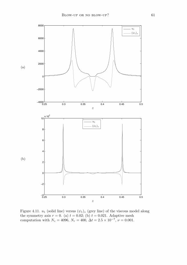
Blow-up or no blow-up? 61
(a)
0.25 0.3 0.35 0.4 0.45 0.5−4000
−2000
0
2000
4000
6000
8000
u1
(ψ1)z
z
(b)
0.25 0.3 0.35 0.4 0.45 0.5−4
−2
0
2
4
6
8
10x 10
4
u1
(ψ1)z
z
Figure 4.11. u1 (solid line) versus (ψ1)z (grey line) of the viscous model alongthe symmetry axis r = 0. (a) t = 0.02; (b) t = 0.021. Adaptive meshcomputation with Nz = 4096, Nr = 400, ∆t = 2.5 × 10⁻⁷, ν = 0.001.
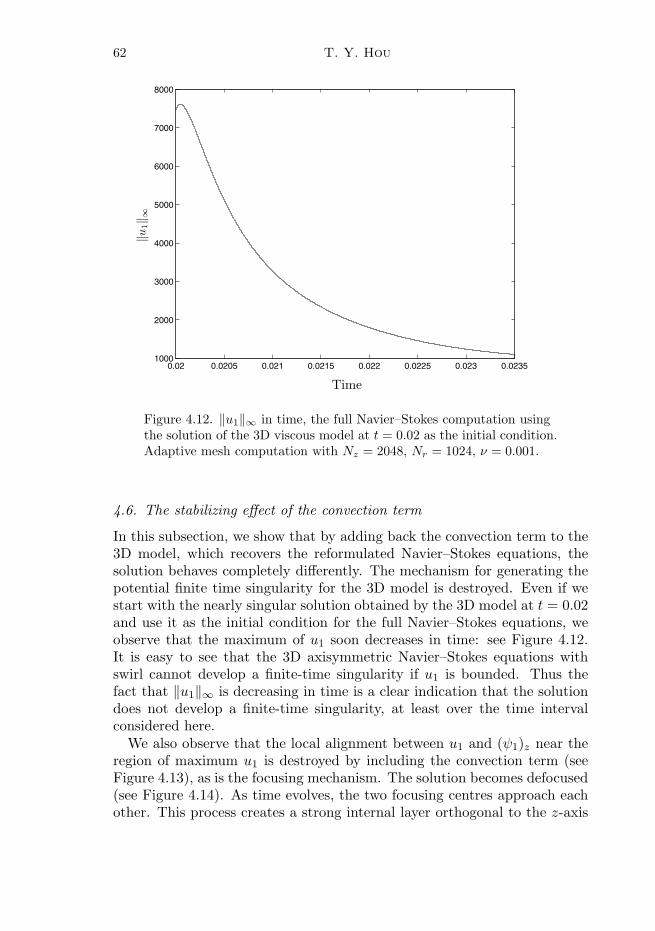
62 T. Y. Hou
0.02 0.0205 0.021 0.0215 0.022 0.0225 0.023 0.02351000
2000
3000
4000
5000
6000
7000
8000
‖u1‖ ∞
Time
Figure 4.12. ‖u1‖∞ in time, the full Navier–Stokes computation usingthe solution of the 3D viscous model at t = 0.02 as the initial condition.Adaptive mesh computation with Nz = 2048, Nr = 1024, ν = 0.001.
4.6. The stabilizing effect of the convection term
In this subsection, we show that by adding back the convection term to the3D model, which recovers the reformulated Navier–Stokes equations, thesolution behaves completely differently. The mechanism for generating thepotential finite time singularity for the 3D model is destroyed. Even if westart with the nearly singular solution obtained by the 3D model at t = 0.02and use it as the initial condition for the full Navier–Stokes equations, weobserve that the maximum of u1 soon decreases in time: see Figure 4.12.It is easy to see that the 3D axisymmetric Navier–Stokes equations withswirl cannot develop a finite-time singularity if u1 is bounded. Thus thefact that ‖u1‖∞ is decreasing in time is a clear indication that the solutiondoes not develop a finite-time singularity, at least over the time intervalconsidered here.
We also observe that the local alignment between u1 and (ψ1)z near theregion of maximum u1 is destroyed by including the convection term (seeFigure 4.13), as is the focusing mechanism. The solution becomes defocused(see Figure 4.14). As time evolves, the two focusing centres approach eachother. This process creates a strong internal layer orthogonal to the z-axis
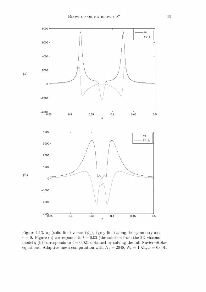
Blow-up or no blow-up? 63
(a)
0.25 0.3 0.35 0.4 0.45 0.5−4000
−2000
0
2000
4000
6000
8000u1
(ψ1)z
z
(b)
0.25 0.3 0.35 0.4 0.45 0.5−3000
−2000
−1000
0
1000
2000
3000
4000u1
(ψ1)z
z
Figure 4.13. u1 (solid line) versus (ψ1)z (grey line) along the symmetry axisr = 0. Figure (a) corresponds to t = 0.02 (the solution from the 3D viscousmodel); (b) corresponds to t = 0.021 obtained by solving the full Navier–Stokesequations. Adaptive mesh computation with Nz = 2048, Nr = 1024, ν = 0.001.
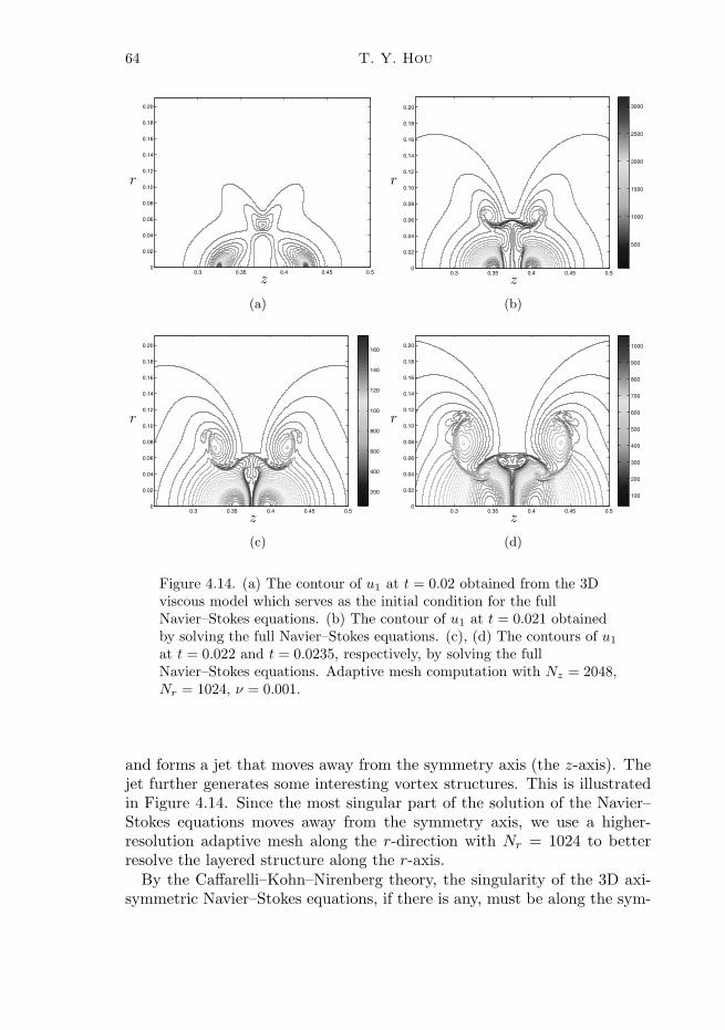
64 T. Y. Hou
0.3 0.35 0.4 0.45 0.50
0.02
0.04
0.06
0.08
0.10
0.12
0.14
0.16
0.18
0.20
r
z
(a)
0.3 0.35 0.4 0.45 0.50
0.02
0.04
0.06
0.08
0.10
0.12
0.14
0.16
0.18
0.20
500
1000
1500
2000
2500
3000
r
z
(b)
0.3 0.35 0.4 0.45 0.50
0.02
0.04
0.06
0.08
0.10
0.12
0.14
0.16
0.18
0.20
200
400
600
800
1000
1200
1400
1600
r
z
(c)
0.3 0.35 0.4 0.45 0.50
0.02
0.04
0.06
0.08
0.10
0.12
0.14
0.16
0.18
0.20
100
200
300
400
500
600
700
800
900
1000
r
z
(d)
Figure 4.14. (a) The contour of u1 at t = 0.02 obtained from the 3Dviscous model which serves as the initial condition for the fullNavier–Stokes equations. (b) The contour of u1 at t = 0.021 obtainedby solving the full Navier–Stokes equations. (c), (d) The contours of u1
at t = 0.022 and t = 0.0235, respectively, by solving the fullNavier–Stokes equations. Adaptive mesh computation with Nz = 2048,Nr = 1024, ν = 0.001.
and forms a jet that moves away from the symmetry axis (the z-axis). Thejet further generates some interesting vortex structures. This is illustratedin Figure 4.14. Since the most singular part of the solution of the Navier–Stokes equations moves away from the symmetry axis, we use a higher-resolution adaptive mesh along the r-direction with Nr = 1024 to betterresolve the layered structure along the r-axis.
By the Caffarelli–Kohn–Nirenberg theory, the singularity of the 3D axi-symmetric Navier–Stokes equations, if there is any, must be along the sym-
Blow-up or no blow-up? 65
metry axis. The fact that the most singular part of the solution moves awayfrom the symmetry axis indicates that the full Navier–Stokes equations willnot form a finite-time singularity, at least not for the initial condition weconsider here over the time interval for which we compute the solution. Onthe other hand, the solution of the 3D model with the same initial conditionseems to develop a potential finite-time singularity in an earlier time. Thisconfirms that convection plays an essential role in depleting the destabilizingeffect induced by vortex stretching.
5. Concluding remarks
Our analysis and computations revealed a subtle dynamic depletion of vor-tex stretching. Sufficient numerical resolution is essential to capture thisdynamic depletion. Our computations for the two antiparallel vortex tubesinitial data showed that the velocity is bounded and that the vortex stretch-ing term is bounded by C‖ω‖L∞ log(‖ω‖L∞). In Hou and Li (2008b), wealso repeated the computation of R. Pelz using highly symmetric initialdata (Pelz 1997). We found that while Pelz’s vortex filament model indeedproduces a finite-time self-similar singularity, the solution of the full 3DEuler equation with the same initial data gives only very modest growthdynamically. No evidence of finite-time singularities was found. Pelz’s vor-tex filament computation was inspired by his earlier computation of the3D Navier–Stokes equations (Boratav and Pelz 1994). However, our com-putation showed that the rapid growth of vorticity observed by Boratavand Pelz (1994) was due to under-resolution of his numerical solution (Houand Li 2008b). The actual growth of maximum vorticity was only expo-nential in the time interval when the solution was still well resolved. It isnatural to ask if the dynamic depletion that we observed is generic, andto consider the driving mechanism for this depletion of vortex stretching.Some recent progress has been made in analysing the dynamic depletionof vortex stretching and nonlinear stability for 3D axisymmetric flows withswirl (Hou and Li 2008a, Hou, Lei and Li 2008). A related study for the 2Dquasi-geostrophic model can be also found in Deng, Hou, Li and Yu (2006b).The local geometric structure of the solution near the region of maximumvorticity and the anisotropic scaling of the support of maximum vorticityseem to play a key role in the dynamic depletion of vortex stretching.
We also studied the dynamic stability of the 3D Navier–Stokes equationsvia an exact 1D model. This 1D model is an exact reduction of the 3DNavier–Stokes equations along the symmetry axis for a special class of initialdata. It retains some essential nonlinear features of the 3D Navier–Stokesequations. We proved the global regularity of this 1D model by using apointwise estimate. The key was to show that a positive Lyapunov function
66 T. Y. Hou
satisfies a new maximum principle. Here convection played an essential rolein cancelling the destabilizing vortex stretching terms. Using the solutionof the 1D model as a building block, we constructed a family of solutionsof the 3D Navier–Stokes equations which experience interesting dynamicgrowth but remain smooth for all times.
To gain further understanding of the stabilizing effect of convection, weconstructed a new 3D model by neglecting the convection term from thereformulated Navier–Stokes equations. This 3D model shares almost allproperties of the Navier–Stokes equations, including an equivalent energyidentity and a partial regularity result. Our numerical results seemed tosupport the conclusion that the solution of the 3D model develops locallyself-similar isotropic singularities. But when we added the convection termback to the 3D model, the mechanism for generating the finite-time singu-larity in the 3D model was destroyed.
The results presented in this paper may have some important implicationto the global regularity of the 3D Navier–Stokes equations. Our studiesindicate that a successful strategy in analysing the global regularity of the3D Navier–Stokes equations need to take advantage of the stabilizing effectof the convection term in an essential way. So far most of the regularityanalysis for the 3D Navier–Stokes equations has not used the stabilizingeffect of the convection term. In many cases, the same results can alsobe obtained for our 3D model. We are currently working to prove thatthe 3D model develops finite-time singularities from smooth initial datawith finite energy. Such a theoretical result would show convincingly thattraditional energy estimates are inadequate to prove global regularity of the3D Navier–Stokes equations. New analytical tools that exploit the localgeometric structure of the solution and the stabilizing effect of convectionwould be needed.
We also investigated the performance of pseudo-spectral methods in com-puting nearly singular solutions of fluid dynamics equations. In particu-lar, we proposed a novel pseudo-spectral method with a high (36th)-orderFourier smoothing which retains a significant portion of the Fourier modesbeyond the 2/3 cut-off point. We demonstrated that the pseudo-spectralmethod with the high-order Fourier smoothing gives a much better per-formance than the pseudo-spectral method with the 2/3 de-aliasing rule.Moreover, we showed that the high-order Fourier smoothing method cap-tures about 12 ∼ 15% more effective Fourier modes in each dimension thanthe 2/3 de-aliasing method. For the 3D Euler equations, the gain in theeffective Fourier codes for the high-order Fourier smoothing method canbe as large as 20% over the 2/3 de-aliasing method. Another interestingobservation was that the error produced by the high-order Fourier smooth-ing method is highly localized near the region where the solution is mostsingular, while the 2/3 de-aliasing method tends to produce oscillations in
Blow-up or no blow-up? 67
the entire domain. The high-order Fourier smoothing method was found bevery stable dynamically. No high-frequency instability was observed.
Acknowledgements
I would like to thank my collaborators, Drs Jian Deng, Zhen Lei, Con-gming Li, Ruo Li, and Xinwei Yu, who have contributed significantly tothe results presented in this survey paper. We would like to thank Prof.Lin-Bo Zhang from the Institute of Computational Mathematics in ChineseAcademy of Sciences (CAS) for providing us with the computing resourcesto perform this large-scale computational project. Additional computingresources were provided by the Center of High Performance Computing inCAS. We also thank Prof. Robert Kerr for providing us with his Fortransubroutine generating his initial data. This work was in part supported bythe NSF under the NSF grant DMS-0713670.
REFERENCES
A. Babin, A. Mahalov and B. Nicolaenko (2001), ‘3D Navier–Stokes and Eulerequations with initial data characterized by uniformly large vorticity’, IndianaUniv. Math. J. 50, 1–35.
J. T. Beale, T. Kato and A. Majda (1984), ‘Remarks on the breakdown of smoothsolutions of the 3-D Euler equations’, Comm. Math. Phys. 96, 61–66.
O. N. Boratav and R. B. Pelz (1994), ‘Direct numerical simulation of transitionto turbulence from a high-symmetry initial condition’, Phys. Fluids 6, 2757–2784.
J. P. Boyd (2000), Chebyshev and Fourier Spectral Methods, 2nd edn, Dover.L. Caffarelli, R. Kohn and L. Nirenberg (1982), ‘Partial regularity of suitable
weak solutions of the Navier–Stokes equations’, Commun. Pure Appl. Math.35, 771–831.
R. Caflisch (1993), ‘Singularity formation for complex solutions of the 3D incom-pressible Euler equations’, Physica D 67, 1–18.
C. Cao and E. S. Titi (2007), ‘Global well-posedness of the three-dimensional prim-itive equations of large scale ocean and atmosphere dynamics’, Ann. of Math.166, 245–267.
D. Chae (2006), ‘Global regularity of the 2d Boussinesq equation with partialviscous terms’, Adv. Math. 203, 497–513.
D. Chae and J. Lee (2002), ‘On the regularity of the axisymmetric solutions of theNavier–Stokes equations’, Math. Z. 239, 645–671.
C. Chen, R. M. Strain, T. Tsai and H. T. Yau (2008), ‘Lower bound on the blow-up rate of the axisymmetric Navier–Stokes equations’, Int. Math. Res. Not.,article ID rnn016.
C. Chen, R. M. Strain, T. Tsai and H. T. Yau (2009), ‘Lower bound on the blow-up rate of the axisymmetric Navier–Stokes equations II’, to appear in Comm.Partial Differential Equations.
68 T. Y. Hou
A. Chorin (1982), ‘The evolution of a turbulent vortex’, Comm. Math. Phys.83, 517.
A. J. Chorin and J. E. Marsden (1993), A Mathematical Introduction to FluidMechanics, 3rd edn, Springer.
P. Constantin (1986), ‘Note on loss of regularity for solutions of the 3-D incom-pressible Euler and related equations’, Comm. Math. Phys. 104, 311–326.
P. Constantin (1994), ‘Geometric statistics in turbulence’, SIAM Review 36, 73.P. Constantin and C. Foias (1988), Navier–Stokes Equations, Chicago University
Press.P. Constantin, C. Fefferman and A. Majda (1996), ‘Geometric constraints on po-
tentially singular solutions for the 3-D Euler equation’, Comm. Partial Dif-ferential Equations 21, 559–571.
P. Constantin, P. D. Lax and A. Majda (1985), ‘A simple one-dimensional modelfor the three-dimensional vorticity equations’, Commun. Pure Appl. Math.38, 715–724.
J. Deng, T. Y. Hou and X. Yu (2005), ‘Geometric properties and non-blowup of3-D incompressible Euler flow’, Comm. Partial Differential Equations 30,225–243.
J. Deng, T. Y. Hou and X. Yu (2006a), ‘Improved geometric conditions for non-blowup of 3D incompressible Euler equation’, Comm. Partial DifferentialEquations 31, 293–306.
J. Deng, T. Y. Hou, R. Li and X. Yu (2006b), ‘Level set dynamics and the non-blow-up of the quasi-geostrophic equation’, Methods Appl. Anal. 13, 157–180.
V. M. Fernandez, N. J. Zabusky and V. M. Gryanik (1995), ‘Vortex intensificationand collapse of the Lissajous-elliptic ring: Single and multi-filament Biot–Savart simulations and visiometrics’, J. Fluid Mech. 299, 289–331.
J. Goodman, T. Y. Hou and E. Tadmor (1994), ‘On the stability of the unsmoothedFourier method for hyperbolic equations’, Numer. Math. 67, 93–129.
R. Grauer and T. Sideris (1991), ‘Numerical computation of three dimensionalincompressible ideal fluids with swirl’, Phys. Rev. Lett. 67, 3511.
R. Grauer, C. Marliani and K. Germaschewski (1998), ‘Adaptive mesh refinementfor singular solutions of the incompressible Euler equations’, Phys. Rev. Lett.80, 19.
T. Y. Hou and Z. Lei (2009a), ‘On the partial regularity of a 3D model of theNavier–Stokes equations’, Comm. Math. Phys. 287, 589–612.
T. Y. Hou and Z. Lei (2009b), ‘On the stabilizing effect of convection for threedimensional incompressible flows’, Commun. Pure Appl. Math. 62, 501–564
T. Y. Hou and C. Li (2005), ‘Global well-posedness of the viscous Boussinesqequations’, Discrete Contin. Dyn. Syst. 12, 1–12.
T. Y. Hou and C. Li (2008a), ‘Dynamic stability of the 3D axi-symmetric Navier–Stokes equations with swirl’, Commun. Pure Appl. Math. 61, 661–697.
T. Y. Hou and R. Li (2006), ‘Dynamic depletion of vortex stretching and non-blowup of the 3-D incompressible Euler equations’, J. Nonlinear Sci. 16, 639–664.
T. Y. Hou and R. Li (2007), ‘Computing nearly singular solutions using pseudo-spectral methods’, J. Comput. Phys. 226, 379–397.
Blow-up or no blow-up? 69
T. Y. Hou and R. Li (2008b), ‘Blowup or no blowup? The interplay between theoryand numerics’, Physica D 237, 1937–1944.
T. Y. Hou, Z. Lei and C. Li (2008), ‘Global regularity of the 3D axi-symmetricNavier–Stokes equations with anisotropic data’, Comm. Partial DifferentialEquations 33, 1622–1637.
L. Iskauriaza, G. Seregin and V. Sverak (2003), ‘L3,∞-solutions of Navier–Stokesequations and backward uniqueness’, Uspekhi Mat. Nauk 58, 3–44.
R. M. Kerr (1993), ‘Evidence for a singularity of the three dimensional, incom-pressible Euler equations’, Phys. Fluids 5, 1725–1746.
R. M. Kerr (2005), ‘Velocity and scaling of collapsing Euler vortices’, Phys. Fluids17, 075103–114.
R. M. Kerr and F. Hussain (1989), ‘Simulation of vortex reconnection’, Physica D37, 474.
G. Koch, N. Nadirashvili, G. Seregin and V. Sverak (2009), ‘Liouville theorems forthe Navier–Stokes equations and applications’, to appear in Acta Mathemat-ica.
H. Kozono and Y. Taniuchi (2000), ‘Bilinear estimates in BMO and Navier–Stokesequations’, Math Z. 235, 173–194.
O. Ladyzhenskaya (1970), Mathematical Problems of the Dynamics of Viscous In-compressible Fluids, Nauka, Moscow.
R. J. LeVeque (1992), Numerical Method for Conservation Laws, Birkhauser.F. H. Lin (1998), ‘A new proof of the Caffarelli–Kohn–Nirenberg theorem’, Com-
mun. Pure Appl. Math. 51, 241–257.J. G. Liu and W. C. Wang (2006), ‘Convergence analysis of the energy and helicity
preserving scheme for axisymmetric flows’, SIAM J. Numer. Anal. 44, 2456–2480.
A. J. Majda and A. L. Bertozzi (2002), Vorticity and Incompressible Flow, Cam-bridge University Press.
R. B. Pelz (1997), ‘Locally self-similar, finite-time collapse in a high-symmetryvortex filament model’, Phys. Rev. E 55, 1617–1626.
G. Prodi (1959), ‘Un teorema di unicita per el equazioni di Navier–Stokes’, Ann.Mat. Pura Appl. 48, 173–182.
A. Pumir and E. E. Siggia (1990), ‘Collapsing solutions to the 3-D Euler equations’,Phys. Fluids A 2, 220–241.
G. Raugel and G. Sell (1993a), ‘Navier–Stokes equations on thin 3D domains I:Global attractors and global regularity of solutions’, J. Amer. Math. Soc.6, 503–568.
G. Raugel and G. Sell (1993b), Navier–Stokes equations on thin 3D domains III:Global and local attractors, in Turbulence in Fluid Flows: A Dynamical Sys-tems Approach, Vol. 55 of IMA Volumes in Mathematics and its Applications,Springer, pp. 137–163.
G. Raugel and G. Sell (1994), Navier–Stokes equations on thin 3D domains II:Global regularity of spatially periodic solutions, in Nonlinear Partial Differ-ential Equations and their Applications, College de France Seminar, Vol. XIof Pitman Research Notes Math, Series 299, Longman, pp. 205–247.
J. Serrin (1962), ‘On the interior regularity of weak solutions of the Navier–Stokesequations’, Arch. Ration. Mech. Anal. 9, 187–195.
70 T. Y. Hou
J. Serrin (1963), The initial value problem for the Navier–Stokes equations, inNonlinear Problems (R. Langer, ed.), University of Wisconsin Press, pp. 69–98.
M. J. Shelley, D. I. Meiron and S. A. Orszag (1993), ‘Dynamical aspects of vortex re-connection of perturbed anti-parallel vortex tubes’, J. Fluid Mech. 246, 613–652.
M. Struwe (1988), ‘On partial regularity results for the Navier–Stokes equations’,Commun. Pure Appl. Math. 41, 437–458.
R. Temam (2001), Navier–Stokes Equations, AMS, Providence, RI.
Online references
C. Fefferman, Clay Mathematical Institute, Millennium Open Problems:www.claymath.org/millennium/Navier–Stokes Equations/