Channel Path-Loss Measurement and Modeling in Wireless ...

EJECE, European Journal of Electrical and Computer Engineering Vol. 4, No. 1, February 2020

DOI: http://dx.doi.org/10.24018/ejece.2020.4.1.157 1

Abstract—Careful network planning has become

increasingly critical with the rising deployment, coverage, and congestion of wireless local area networks (WLANs). This paper investigates and determine the Path-loss exponent value for the ubiquitous wireless local area network at the Federal University Oye-Ekiti for the line of sight and non-line of sight (N-LOS). Aside this, the paper also models the wireless network using artificial neural network (ANN) technology by training some neurons based on data collected from a drive-test.

The proposed ANN model performed with accuracy and is offered as a simple, yet strong predictive model for network planning – having both speed and accuracy. Results show, that for the area under study, Oye Campus has a higher standard deviation of 5.76dBm as against ikole Campus with 1.44dBm, this is because of dense vegetation at Oye Campus.

In view of this, the paper provides a predictive site survey for rapid wireless Access point deployment.

Index Terms—Artificial Neural Network, N-LOS, Path Loss, Propagation Model.

I. INTRODUCTION Path Loss is difference in dB between transmitted signal

and received signal strength at a location. Network Engineers mostly used path loss model as a mathematical tool to determine received signal strength at a given point. The problem of predicting propagation loss between two points may be seen as a function of several inputs and a single output. The inputs contain information about the transmitter and receiver locations, surrounding buildings, frequency, etc. while the output gives the propagation loss for those inputs. From this point of view, research in propagation loss modeling consists of finding both the inputs and the function that best approximate the propagation loss. The various models that have been proposed can be classified as empirical or deterministic model. Empirical models like ITU, TGn, SUI and Okumura-Hata[12]-[13], [17], [20] are based on received signal measurement within a given environment. The Empirical models are computationally efficient but may not be very accurate in different environment. Deterministic models like geometric theory of wave, ray-tracing [8][9] technology is very accurate but requires extensive computational time and

Published on February 27 , 2020. O. Y. Olajide, Department of Electrical/Electronic Engineering, Federal

University of Technology Akure, Nigeria. (e-mail: [email protected]) Y. M. Samson, ICT UNIT, Federal University Oye-Ekiti, Nigeria. (e-mail: [email protected])

detailed information of the environment. The introduction of Machine learning techniques has

helped in solving complex problems in our everyday life, this can be exploited for path loss predictions in given propagation environments. Artificial Neural Network (ANN) is an adaptive statistical tool that models the biological nervous system to solve regression problems. The capability of ANNs to model complex nonlinear functional relationships provides an opportunity to combine the gains of empirical and deterministic models and also to provide better computational efficiency. ANN has high processing speed and can process large volume of data, has the flexibility to adapt to different environments and can be trained to perform well in environments similar to where the training data are collected. The basic features of the ANN are for it to be able to create its own internal model of behavior of radio waves by observing the measured data, measured data have inherent behavior of the network from where it was collected, as such the measured data are needed for the creation of ANN model. The feed-forward neural networks [4], [5] are very well suited for prediction purposes because they do not allow any feedback from the output (field strength or path loss) to the input. ANN can be used to model the mathematical function of Pathloss of a given environment.

II. RELATED LITERATURE

A. Stanford University Interim (SUI) Model [2], [21] The 802.16 IEEE group, jointly with the Stanford

University, carried out an extensive work with the aim to develop a channel model for WiMAX applications in suburban environments. The model is formulated to operate based on an operating frequency above 1900MHz and a cell radius of 0.1km to 8km, base station antenna height 10m to 80m, and receiver antenna height of 1m to 10m. This model is divided into three categories of terrains namely A, B, C. The terrain category A is associated with maximum path loss, and densely populated region. Moderate path loss is captured in terrain category B. The terrain category C is associated with minimum path loss and flat terrain with light tree densities.

The basic path loss expression of The SUI model with correction factors is presented as:

𝑃𝐿 = 𝐴 + 10𝛾 log!" ,

##!- + 𝑋$ + 𝑋% + 𝑠𝑑 > 𝑑" (1)

Channel Path-Loss Measurement and Modeling in Wireless Data Network (IEEE 802.11n) Using Artificial

Neural Network

Olasoji Y. Olajide and Yerima M. Samson



where 𝑑is the distance between BS and receiving antenna (m), 𝑑"is the reference distance 100 (m),𝑋$is the frequency correction factor for frequency above 2 GHz, 𝑋%is the correction factor for receiving antenna height (m), 𝑠is the correction for shadowing (dB), and𝛾 is the path loss exponent. The random variables are taken through a statistical procedure as the path loss exponent γ and the weak fading standard deviation s is defined. The log normally distributed factor𝑠, for shadow fading because of trees and other clutter on a propagations path and its value is between 8.2 dB and 10.6 dB. The parameter A is defined as:

𝐴 = 20 log!" ,

'(#!)- (2)

The frequency correction factor𝑋$ and the correction for

receiver antenna height𝑋% for the model are expressed in:

𝑋$ = 6.0 log!" ,$

*"""- (3)

For terrain type A and B

𝑋% = −10.8 log!" ,

%"*"""

- (4)

for terrain type C

𝑋% = −20 log!" ,%"*"""

- (5)

Where 𝑓is the operating frequency (MHz), ℎ+ is the receiver antenna height (m)

For the above correction factors this model is extensively used for the path loss prediction of all three types of terrain in rural, urban and suburban environments.

B. IEEE 802.11 TGn channel model The TGn channel model was conceived for systems with

4x4 MIMO, and are based on the Kronecker channel correlation model assumption. According to the IEEE 802.11 TGn channel model, the PL can be modeled by the free space PL for d < d", and by a one-slope model with exponent 3.5 for d > d". The TGn model predicts a breakpoint of 5m for ‘Small environment’ (type of environment ‘C’) and a breakpoint of 10m for ‘Large environment’ (type of environment ‘D’).

PL(d) = PL,-.(0)d ≤ d" (6)

PL(d) = PL,23(d") + 35 log!" ,

00!- d > d" (7)

where d is the transmit-receive separation distance in m. the standard deviations of log-normal (Gaussian in dB) shadow fading were found to be in the 3-14 dB range. PLLOS(d)= Free path loss

C. COST 231 Walfish-Ikegami (W-I) Model [17], [20], [15] This model is a combination of J. Walfish and F. Ikegami

models. This model is considered as the most appropriate model for rural and suburban environments which have regular building height. Among other models like the Hata model, COST 231 W-I model gives a more precise path loss. This is as a result of the additional parameters introduced which characterized the different environments. It distinguishes different terrain with different proposed parameters. The equation of the proposed model is expressed in:

For LOS condition

𝑃𝐿456 = 42.6 + 26 log!"(𝑑) + 20 log!"(𝑓) (8)

And for NLOS condition

𝑃𝐿!"#$ = $𝐿%&' + 𝐿()& + 𝐿*&+ , forurbanandsuburban

𝐿%&' ,𝐿()& + 𝐿*&+ < 0(9)

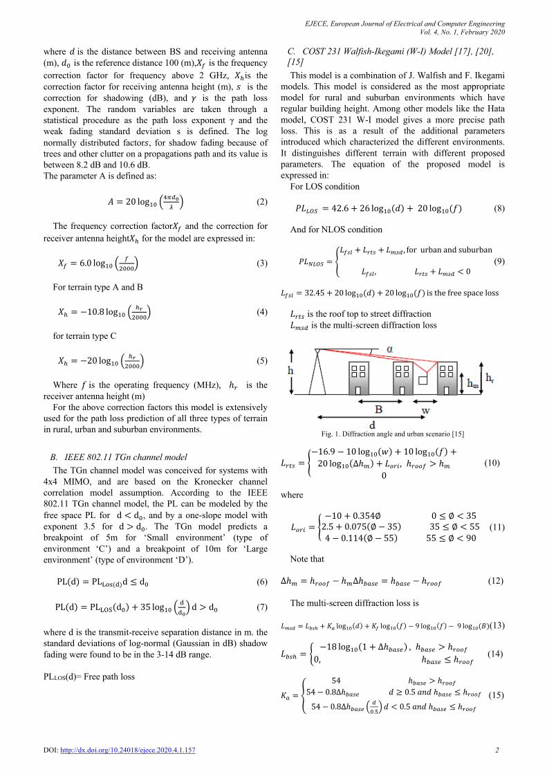
𝐿%&' = 32.45 + 20 log,-(𝑑) + 20 log,-(𝑓) isthefreespaceloss 𝐿+78 is the roof top to street diffraction 𝐿98# is the multi-screen diffraction loss

Fig. 1. Diffraction angle and urban scenario [15]

𝐿+78 = D−16.9 − 10 log!"(𝑤) + 10 log!"(𝑓) +20 log!"(∆ℎ9) + 𝐿:+; , ℎ+::$ > ℎ9

0 (10)

where

𝐿:+; = D−10 + 0.354∅0 ≤ ∅ < 352.5 + 0.075(∅ − 35)35 ≤ ∅ < 554 − 0.114(∅ − 55)55 ≤ ∅ < 90

(11)

Note that

∆ℎ9 = ℎ+::$ − ℎ9∆ℎ<=8> = ℎ<=8> − ℎ+::$ (12)

The multi-screen diffraction loss is

𝐿!"# = 𝐿$"% + 𝐾& log'((𝑑) + 𝐾) log'((𝑓) − 9 log'((𝑓) − 9 log'((𝐵)(13)

𝐿<8% = K−18 log!"(1 + ∆ℎ<=8>) , ℎ<=8> > ℎ+::$0, ℎ<=8> ≤ ℎ+::$

(14)

𝐾. = E

54ℎ/.&0 > ℎ(11%54 − 0.8∆ℎ/.&0𝑑 ≥ 0.5𝑎𝑛𝑑ℎ/.&0 ≤ ℎ(11%54 − 0.8∆ℎ/.&0 O

+-.3P𝑑 < 0.5𝑎𝑛𝑑ℎ/.&0 ≤ ℎ(11%

(15)



𝐾# = D18, ℎ<=8> > ℎ+::$

18 − 15 ,∆%#$%&%#$%&

- , ℎ<=8> ≤ ℎ+::$ (16)

For suburban or medium size cities with moderate tree

density

𝐾$ = −4 + 0.7 , $@*A

− 1- (17)

And for metropolitan – urban

𝐾$ = −4 + 1.5 , $@*A

− 1- (18)

where 𝑑is the distance between transmitter and receiver antenna

(m) 𝑓 is the frequency (GHz) 𝐵 is the building to building distance (m) 𝑤is the street width (m) ∅is the street orientation angel with respect to direct

radio path (degree)

D. ITU Model [10], [17], [19], [12] The International Telecommunication Union Radio

communication (ITU-R) is a semi empirical path loss model that can be employed in different environment comprising indoor, outdoor, vehicular and pedestrian. The applicable operational frequency is 900MHz – 6GHz and the equations for the line of sight (LOS) and non-LOS (NLOS) path loss are;

𝑃B(456) = 18 log!"(𝑓C) + 𝑁 log!"(𝑑) − 28 (19)

𝑃B(D456) = 20 log!"(𝑓C) + 𝑁 log!"(𝑑) + 𝐿𝑓(𝑛E) − 28 (20)

Where; 𝑓C= carrier frequency in MHz N= Power Loss

Coefficient d= Tx-Rx distance in meters Lf= wall penetration loss 𝑛E =the number of walls

E. Calculation of distance power loss coefficient The distance power loss coefficient, N is the quantity that

expresses the loss of signal power with distance. This coefficient is an empirical one. Some values are provided in Table I.

TABLE I: [12]

Frequency band Residential area Office

area Commercial area

900 MHz N/A 33 20 1.2–1.3 GHz N/A 32 22 1.8–2.0 GHz 28 30 22 4 GHz N/A 28 22

5.2 GHz 30 (apartment), 28 (house) 31 N/A

5.8 GHz N/A 24 N/A 6.0 GHz N/A 22 17

F. Calculation of floor penetration loss factor The floor penetration loss factor is an empirical constant

dependent on the number of floors the waves need to penetrate. Some values are tabulated in Table II.

TABLE II: [12]

III. DATA COLLECTION METHOD AND ANALYSIS Pathloss model prediction for wireless data network

requires practical data from the field measurement. Received signal strength were measured at various distances from the transmitter at the ISM band frequency of 2400MHz. A drive test tools for data collection includes a laptop equipped with communication Network/Protocol Analyser (metageek insider 4 software) and GPS receiver to measure the longitude and latitude of the received signal. The average transmitted power from the transmitter is 28 dBm. Results obtained was plot in MATLAB.

Designing ANN models follows a number of systemic procedures. In general, there are five basic steps: (1) data collection, (2) data preprocessing, (3) Network Building, (4) training and (5) model performance test as shown below.

Fig. 2. Basic flow for ANN Model Designing

The work presented in this paper is modeled using

McCulloch-Pitts model. The MATLAB [1][3][5] tools contain the Neural Network Toolbox [4] for designing, implementing, visualizing and simulating neural networks. It also provides comprehensive support for many proven network paradigms, as well as graphical user interfaces (GUIs) that enable the user to design and manage neural networks in a very simple way.

Fig. 3. McCullouch-Pitts Model of ANN

Y=F(∑ (𝑤+ ∗ 𝑝+ + 𝑏)+

+F! ) (21)

p = (p1, …, pr) is the input column-vector W = (w1, …, wr) is the weight row-vector F=the transfer function The bias b can be treated as a weight whose input is

always 1.

Data Collection Preprocessing Building Network

Training

Network

Testing Network

Frequency band

Number of floors

Residential area Office area Commercial

area 900 MHz 1 N/A 9 N/A 900 MHz 2 N/A 19 N/A 900 MHz 3 N/A 24 N/A 1.8–2.0 GHz n 4n 15+4(n-1) 6 + 3(n-1)

5.2 GHz 1 N/A 16 N/A

5.8 GHz 1 N/A 22 (1 floor), 28 (2 floors) N/A



IV. PATHLOSS MEASUREMENT AND RESULTS The path loss measurement was taken at the Ikole and

Oye campus of the Federal University Oye-Ekiti Ekiti State Nigeria. The two campuses consist of structures and foliage. The measurements were done at the ISM band frequency 2.4GHz. The transmitter used is the ZoneFlex_9.7 802.11n Outdoor Access Point [6]. The receiver equipment included a laptop, equipped with LB LINK™ BL-WN150 WLAN USB adapter card and inSSIDer Wi-Fi network scanner/protocol analyzer. The receiver was moved around the campus for the received power in dBm and the longitude/latitude position of the receiver was recorded. Haversine formula was used to calculate the distance between the transmitter and the receiver given the longitude/latitude.

This work concentrated on the received radio signal needed for the path loss analysis of the coverage area. The path loss includes signal attenuation with signal fading between the transmitter and the receiver, while the channel consists of structures and foliage. It is to be noted that while conducting the drive test other WiFi AP acted as interference to the received signal.

Fig. 4. Google Earth view of Oye campus

Fig. 5. Google Earth view of Ikole Campus

TABLE III: AP POSITION IKOLE CAMPUS

AP NAME LONGITUDE LATITUDE MechaEng AP 5 29’ 38.20”E 7 48’ 27.65”N Civil Eng AP 5 29’ 35.98”E 7 48’ 27.63”N Dean Eng AP 5 29’ 37.11”E 7 48’ 26.72”N Dean Agric AP 5 29’ 49.41”E 7 48’ 13.72”N

TABLE IV: AP POSITION OYE CAMPUS

AP NAME LONGITUDE LATITUDE ICT New AP 5 18’ 42.75”E 7 46’ 34.70”N Fac of sci AP 5 18’ 55.58”E 7 46’ 37.24”N Theater AP 5 18’ 59.73”E 7 46’ 35.96”N Science1 AP 5 18’ 15.78”E 7 46’ 37.14”N

Science2 AP 5 18’ 55.28”E 7 46’ 36.96”N

The measured received power in both campuses are plotted in Fig. 6, while the path loss are plotted in Fig. 7. By observing the path loss values, it was clear that the path loss deviation has less value at Ikole campus than Oye campus, this is due to less foliage and structures at Ikole campus than Oye campus as seen in the Google Earth view map.

Fig. 6. Measured Received Power

Fig. 7. Path Loss Using Measured Data

Fig. 8. Path Loss include one Slope Model

A. Determination of Power exponent and log-normal variation Average Transmitted power from the AP datashet,

Pt=28dBm.



Average received power from the AP d0=1m,

𝑃+ = −11𝑑𝐵𝑚,𝑘 = 𝑃7 − 𝑃+ = 39𝑑𝐵𝑚 (22)

Using the one slope model to determine the power exponent 𝛾

Let

𝑀!*#+,(𝑑) = 𝑃-(𝑑𝐵𝑚) − 𝑃.(𝑑𝐵𝑚) = 𝐾(𝑑𝐵𝑚) + 10𝛾𝑙𝑜𝑔'( 9##!: + 𝜓/

(23) 𝜓G = zero-mean Gaussian distributed random variable

(in dBm) with standard deviation 𝜎 (also in dBm) minimum mean square error (MMSE) equation for the

dBm power measurements is

𝐹(𝛾) = ∑ ⌈𝑀9>=8H+>#(𝑑;) −𝑀9:#>B(𝑑;)⌉*I;F! (24)

𝐹(𝛾) =ST𝑀*0.&4(0+(𝑑5) − (𝐾(𝑑𝐵𝑚) + 10𝛾𝑙𝑜𝑔,- \𝑑5𝑑-])^

67

58,

𝐹(𝛾) = ∑ `𝑀*0.&4(0+(𝑑5) − 𝐾(𝑑𝐵𝑚) − 10𝛾𝑙𝑜𝑔,- O

+!+"Pa67

58, (25) MMSE occur at 0J(K)

0K= 0

𝛾 = ∑ [N'&$%("&)(#*)OP(#Q9)]

+*,-

∑ [!"B:S-!T)*)!U]+

*,- (26)

Ikole campus n=93, ∑ [𝑀9>=8H+>#(𝑑;)]I;F! =summation of PL=7681.5,

∑ [10𝑙𝑜𝑔!" ,#*#!-]I

;F! = 𝑑𝑖𝑠𝑡𝑎𝑛𝑐𝑒𝑠𝑢𝑚𝑚𝑎𝑡𝑖𝑜𝑛 =1330.013

𝛾 =(7681.5 − 93𝑥39)

1330.013 = 3.05

Oye campus n=184, ∑ [𝑀9>=8H+>#(𝑑;)]I

;F! =summation of PL=15631 ∑ [10𝑙𝑜𝑔!" ,

#*#!-]I

;F! = 𝑑𝑖𝑠𝑡𝑎𝑛𝑐𝑒𝑠𝑢𝑚𝑚𝑎𝑡𝑖𝑜𝑛 =2756.47

𝛾 =(15631 − 184𝑥39)

2756.47 = 3.06 The log-normal variation or shadow fading is giving by

𝜓G =1𝑛h

⌈𝑀9>=8H+>#(𝑑;) −𝑀9:#>B(𝑑;)⌉*I

;F!

Ikole Campus

𝜓9 =1𝑛S

⌈𝑀*0.&4(0+(𝑑5) −𝑀*1+0'(𝑑5)⌉6 =191.4893 = 2,06

7

58,

Standard deviation σ =i𝜓G =√2.06= 1.44𝑑𝐵𝑚 Oye Campus

𝜓9 =1𝑛S

⌈𝑀*0.&4(0+(𝑑5) −𝑀*1+0'(𝑑5)⌉6 =7

58,

6114.27184 = 33.23

Standard deviation σ =i𝜓G =√33.23= 5.76𝑑𝐵𝑚

TABLE V: RESULT OBTAINED

Freq (Ghz)

Location

𝑲 (𝒅𝑩𝒎)

PL Exponent

σ (dBm)

Tx-Rx Distance(m)

2.4 Ikole 39 3.05 1.44 1-100 2.4 Oye 39 3.06 5.76 1-100

V. ANN MODELING AND RESULTS COMPARISON WITH THE FOUR EXISTING MODELS

IEEE802.11n is a fixed wireless network, therefore the ANN model presented in this paper has the following parameters: distance between WiFi AP and the receiver, carrier frequency, height of the WiFi AP and height of the receiver. Set of path loss data recorded at distances between transmitter and receiver were used in the training of the neurons. Levenberg-Marquardt (trainlm) algorithm was used to train the network, this algorithm is generally faster than the others and very ideal for the network model. During the training phase the characteristics of the network were modified by this iterative algorithm until a minimum error is obtained, that is the error between the network (predicted) output and the desired (measured) output is minimized. Observations were made during the training process. It was observed that different results were obtained each time the network was trained. This is as a result of different initial weight and bias values, and different divisions of measured data into training, validation and test sets, thus it is possible that different artificial neural structures trained on the same problem can generate different outputs for the same input. Another observation noted was that network sensitivity depends on the number of neurons in the hidden layer. When the number is few it leads to underfitting but when the number is too many it causes overfitting, the number of hidden layers was varied during training until the desired result was obtained. To achieve the modeling of the network using McCulloch-pitts model, two hidden layer of size five (5) was obtained as the best representation of the network.

Fig. 9. Training the ANN



Fig. 10. Result Performance

The various weights and bias are given below:

IW{1,1}- WEIGHT TO LAYER 1 FROM INPUT 1 -7.0587 -8.3286 -7.5125 -5.7149 6.440

IW{2,1}-WEIGHT TO LAYER

1.4840 -1.1689 1.8698 1.2639 1.3860 0.6068 -2.3206 -0.8896 -0.6184 -0.9326 1.4892 1.0294 -0.3789 0.0312 -2.1822 -1.2016 -0.5139 0.4895 2.5840 -0.0674 0.6244 0.4632 1.1968 0.2990 1.0982

IW{3,1}-WEIGHT TO LAYER

0.5657 0.9578 1.7526 0.2508 0.9772

B{1}- BIAS TO LAYER 1 6.9731 2.6584 0.6378 -3.2609 7.8763

B{2}- BIAS TO LAYER 2

-1.7008 -0.7874 0.1788 -1.2809 2.2889

B{3}- BIAS TO LAYER 3 [-0.23941]

From the ANN analysis the proposed mathematical

function for the wireless data network Path loss is given 𝑃𝐿 = 0.61𝑧A − 0.87𝑧' − 0.88𝑧V − 0.76𝑧* + 8.4𝑧 + 𝐴 (27)

where 𝐴 = 10𝛾 log!"l./)!012 m + 24 (28) 𝑧 = (#OVA)

WX (29)

𝑃𝐿 represent the channel modeling of the wireless data

network in mathematical function, where: 𝛾= the Path Loss coefficients of the environment (3.05-

3.06) 𝑓C= ISM band frequency (2.4GHz to 2.5GHz) 𝑑= distance between the Tx and Rx The model proposed is to be site-general, the radio

transmission loss is characterized by both an average transmission loss and its associated shadow fading statistics. The model proposed in this research accounts for the loss through multiple floors to allow for such characteristics as frequency reuse between floors. The distance power loss coefficients include an implicit allowance for transmission through walls and over and through obstacles, and for other loss mechanisms likely to be encountered within a single floor of a building.

Fig. 11. Comparison of proposed ANN Model with Industry Standard

VI. DISCUSSION From Fig. 11, the proposed ANN model matches closer

with the average drive test data as compared to other models, the zero-mean Gaussian distribution is within the range of 2.06-33.32 dBm, while standard deviation ranges from 1.44dBm to 5.76dBm and the path loss exponent ranges from 3.05-3.06. it was observed from Fig 11 that the ITU model has the highest value of Path loss at 2400 MHz. compared to other models in the same environment, this is as a result of the floor penetration loss factor given in Table V for the number of floors between Access Point and the receiver. It was also observed that at a distance less than 70m the pathloss is approximately linearly depended on the distance, above 70m fading and signal attenuation drastically affect the Pathloss. This result shows that for a good signal connection in wireless data connection distance between Tx and Rx should be less than 70m. From this observation, it could be concluded that the ANN model is statistically a better model compared to others and can be used as a better estimator of path loss for university campuses in Nigeria

VII. CONCLUSION The research goal was to analyze the behavior of

propagation channel, determine the Path loss exponent and to model the channel using ANN for wireless data communication systems operation at ISM 2.4GHz. Based on several drive tests conducted. A mathematical model was formulated which could be used in the deployment of WiFi AP due to its adaptive nature. The propose ANN new model explains the relationship between the path-loss coefficient, the distance between Tx-Rx and the frequency, together produces a novel framework that describe the Path Loss. It provides the basis for the realization of wireless data communication under complicated environment with complex utilizing of the spectrum resource. The ANN model can be used for regular IoT deployment, VOIP, and robotics operating in the ISM band 2.4GHz frequency. As a future work, it is intended that the path loss model for IEEE802.11ac with frequency band of 5GHz will be examined.



REFERENCES [1] Albrecht Schmidt 2000, TECO, viewed 16/4/2013,

http://www.teco.edu/~albrecht/neuro/html/node7. html [2] Caleb Phillips, Douglas Sicker and Dirk Grunwald. “A Survey of

Wireless Path Loss Prediction and Coverage Mapping Methods”. IEE Communications Surveys & Tutorials, vol. 15, no. 1, first quarter 2013

[3] Carnevale and Hines 2013, Neuron, Yale, Viewed 3/05/13, http://neuron.yale.edu/neuron/what_is_neuron

[4] Demuth, H. and Beale, M. 2013, ‘Neural Network Toolbox -User guide’, The MathWorks Inc., PDF

[5] Fausett 1994, “Fundamentals of Neural Networks: Architectures, Algorithms and Applications”, Prentice-Hall, New Jersey, USA.

[6] (https://support.ruckuswireless.com/documents/409-zoneflex-9-7-outdoor-access-point-user guide/download)

[7] Motoharu Sasaki, Minoru Inomata, WataruYamada,TakeshiOnizawa. “Path Loss Models for Wireless Access Network Systems Using High Frequency Bands”.NTT Technical Review.Vol. 14 No. 12 Dec. 2016

[8] T.K. Sarkar, Z. Ji, K. Kim, A. Medouri, and M. Salazar-Palma, “A Survey of Various Propagation Models for Mobile Communications”. IEEE Antennas and Propagation Magazine, Vol. 45, No. 3, June 2003, pp. 51 – 82.

[9] S. R. Saunders, and F. R. Bonar, “Prediction of Mobile Radio Wave Propagation Over Buildings of Irregular Heights and Spacings,” IEEE Transactions on Antennas and Propagation, vol. 42, no. 2, Feb. 1994, pp. 137 – 144.

[10] G.D. Durgin, T. S. Rappaport, and H. Xu, “Measurements and Models for Radio Path Loss and Penetration Loss In and Around Homes and Trees at 5.85 GHz,” IEEE Transactions on Communications, vol. 46, no. 11, November 1998, pp. 1484 – 1496.

[11] Haykin, S. (2009). Neural Networks and Learning Machines. 3rd edition, PearsonEducation,Inc.,New Jersey.

[12] Propagation data and prediction methods for the planning of indoor radio communication systems and radio local area networks in the frequency range 300 MHz to 450 GHz, Recommendation ITU-R P.1238-10 (08/2019).

[13] Theodore S. Rappaport, “Wireless Communication Principles and Practice Second edition”, 2002 chapter (2-4).

[14] M. Inomata, W. Yamada, M. Sasaki, M. Mizoguchi, K. Kitao, and T. Imai, “Path Loss Model for the 2 to 37 GHz Band in Street Microcell Environments,” IEICE Commun. Express, Vol. 4, No. 5, pp. 149–154, 2015.

[15] Yazan A Alqudah, “Performance of Cost 231 Walfish Ikegami Model in Deployed 3.5 GHz Network,” https://www.researchgate.net/publication/255172908, May,2013.

[16] Nafaa M. Shebani,Abdulati E. Mohammed,Mohammed A. Mosbah, Yousra A. Hassan. Simulation and Analysis of Path Loss Models for WiMax Communication System. ISBN: 978-0-9853483-3-5©2013 SDIWC. https://www.researchgate.net/publication/269222079

[17] Yahia Zakaria, Jiri Hosek and Jiri Misurec.Path Loss Measurements for Wireless Communication in Urban and Rural Environments. American Journal of Engineering and Applied Sciences 2015, 8 (1): 94.99 DOI: 10.3844/ajeassp.2015.94.99

[18] Abhayawardhana, V.S., I.J. Wassell, D. Crosby, M.P. Sellars and M.G. Brown, 2005. Comparison of empirical propagation path loss models for fixed wireless access systems. Proceedings of the 61th IEEE Vehicular Technology Conference, May 30-Jun. 1, IEEE Xplore Press, Sweden, pp: 73-77. DOI: 10.1109/VETECS.2005.1543252

[19] Alam, M.D., S. Chowdhurz and S. Alam, 2014. Performance evaluation of different frequency bands of Wi-MAX and their selection procedure. Int. J. Adv. Sci. Technol., 62: 1-18. DOI: 10.14257/ijast.2014.62.01

[20] B.O.H Akinwole, Esobinenwu C.S. Adjustment of Cost 231 Hata Path Model For Cellular Transmission in Rivers State.IOSR Journal of Electrical and Electronics Engineering (IOSR-JEEE) e-ISSN: 2278-1676,p-ISSN: 2320-3331, Volume 6, Issue 5 (Jul. - Aug. 2013), PP 16-23 www.iosrjournals.org.

[21] JalelChebil, Ali K. Lawas and M.D. Rafiqul Islam “Comparison Between Measured andPredicted Path Loss for Mobile Communication in Malaysia”World Applied Sciences Journal 21 (Mathematical Applications in Engineering): 123-128, 2013 ISSN 1818-4952,© IDOSI Publications, 2013 DOI: 10.5829/idosi.wasj.2013.21.mae.99936

Olasoji Y. Olajide (PhD) is with the Department of Electrical/Electronic Engineering, Federal University of Technology Akure, Nigeria (e-mail: [email protected]).

Yerima Musa Samson is with the ICT UNIT, Federal University Oye-Ekiti, Nigeria (e-mail: [email protected].

Channel Path-Loss Measurement and Modeling in Wireless ...

Documents

Transcript of Channel Path-Loss Measurement and Modeling in Wireless ...