MacCartney, G.R., Zhang, J., Nie, S., Rappaport, T.S., IEEE Global Communications Conference, Exhibition & Industry Forum (GLOBECOM), Dec. 9~13, 2013.

Path Loss Models for 5G Millimeter Wave Propagation Channels in Urban Microcells

George R. MacCartney Jr., Junhong Zhang, Shuai Nie, and Theodore S. Rappaport NYU WIRELESS

Polytechnic Institute of New York University Brooklyn, NY 11201

tsr@nyu.edu

Abstract— Measurements for future outdoor cellular systems at 28 GHz and 38 GHz were conducted in urban microcellular environments in New York City and Austin, Texas, respectively. Measurements in both line-of-sight and non-line-of-sight scenarios used multiple combinations of steerable transmit and receive antennas (e.g. 24.5 dBi horn antennas with 10.9° half power beamwidths at 28 GHz, 25 dBi horn antennas with 7.8° half power beamwidths at 38 GHz, and 13.3 dBi horn antennas with 24.7° half power beamwidths at 38 GHz) at different transmit antenna heights. Based on the measured data, we present path loss models suitable for the development of fifth generation (5G) standards that show the distance dependency of received power. In this paper, path loss is expressed in easy-to-use formulas as the sum of a distant dependent path loss factor, a floating intercept, and a shadowing factor that minimizes the mean square error fit to the empirical data. The new models are compared with previous models that were limited to using a close-in free space reference distance. Here, we illustrate the differences of the two modeling approaches, and show that a floating intercept model reduces the shadow factors by several dB and offers smaller path loss exponents while simultaneously providing a better fit to the empirical data. The upshot of these new path loss models is that coverage is actually better than first suggested by work in [1], [7] and [8].

Keywords—28 GHz; 38 GHz; 5G; millimeter wave; statistical spatial channel model; path loss model; shadow fading; channel sounder; cellular standard

I. INTRODUCTION The increasing demand for faster data rates and more

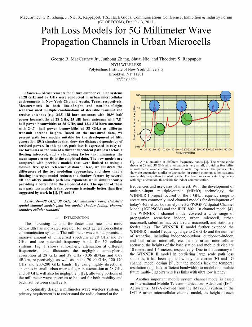
bandwidth has motivated research for next generation cellular communication systems. The millimeter wave bands promise a massive amount of unlicensed spectrum at 28 GHz and 38 GHz, and are potential frequency bands for 5G cellular systems. Fig. 1 shows atmospheric attenuation at different frequencies, and illustrates the negligible atmospheric absorption at 28 GHz and 38 GHz (0.06 dB/km and 0.08 dB/km, respectively), as well as in the 70-90 GHz, 120-170 GHz and 200-280 GHz bands. By using highly directional antennas in small urban microcells, rain attenuation at 28 GHz and 38 GHz will also be negligible [1][2], allowing portions of the millimeter wave spectrum to be used for both mobility and backhaul between small cells.

To optimally design a millimeter wave wireless system, a primary requirement is to understand the radio channel at the

Fig. 1. Air attenuation at different frequency bands [3]. The white circle shows at 28 and 38 GHz air attenuation is very small, providing feasibility of millimeter wave communication at such frequencies. The green circles show the attenuation similar to attenuation in current communication systems, comparably larger than the white circle. The blue circles indicate frequencies with high attenuation, thus viable for indoor communication.

frequencies and use-cases of interest. With the development of multiple-input multiple-output (MIMO) technology, the WINNER I project focused on the 5 GHz frequency range to create two commonly used channel models for development of today's 4G networks, namely the 3GPP/3GPP2 Spatial Channel Model (3GPPSCM) and the IEEE 802.11n channel model [4]. The WINNER I channel model covered a wide range of propagation scenarios: indoor, urban microcell, urban macrocell, suburban macrocell, rural macrocell, and stationary feeder links. The WINNER II model further extended the WINNER I model frequency range to 2-6 GHz and the number of scenarios, including indoor-to-outdoor, outdoor-to-indoor, and bad urban microcell, etc. In the urban microcellular scenario, the heights of the base station and mobile device are 10 meters and 1.5 meters, respectively. Due to the accuracy of the WINNER II model in predicting large scale path loss statistics, it has been applied widely for current 3G and 4G channel model design [5], but the models lack the temporal resolution (e.g. lack sufficient bandwidth) to model or simulate future multi-Gigabit/s wireless links with ultra low latency.

Another important mobile system channel model is based on International Mobile Telecommunications-Advanced (IMT-A) systems. IMT-A evolved from the IMT-2000 system. In the IMT-A urban microcellular channel model, the height of each

base station is 10 meters. Users are randomly and uniformly distributed with base station to mobile station inter-site distances between 10 and 200 meters [6]. The IMT-A channel model has also been used for current 4G systems.

Recently, researchers have focused on abundant millimeter wave spectrum as a potential candidate for 5G cellular systems, yet only a few channel measurement campaigns have been conducted to understand this frequency regime [1][2][7][8][9][10][11]. To generate reliable models for future mm-wave system design, path loss models must be built for link budget and signal strength prediction, with the inclusion of directional and beamforming antenna arrays. NYU WIRELESS researchers have performed extensive propagation measurements in both New York City and Austin, Texas to collect channel model statistics at 28 GHz and 38 GHz [1][2][7][8][10][11]. The empirically based channel statistics from typical urban environments were analyzed to build path loss models, and subsequent work has shown how multiple beams can provide cell coverage extension up to 80% when four coherent beams are combined [12]. In these early urban microcellular path loss models at 28 GHz and 38 GHz, the maximum cell radius was found to be 200 meters using a single 10-degree beamwidth antenna with end users randomly and uniformly distributed over the areas. The two measurement campaigns suggest that a brand-new regime for millimeter wave communication will be viable, and will need to rely on high gain directional steerable antennas for MIMO or beamforming [1][2][7][8][9][10][11][12].

This paper is organized as follows: Section II and III describe the hardware system and measurement scenarios for data collection. Section IV introduces the new millimeter wave propagation channel large scale path loss models for urban microcellular environments, using a floating intercept. In Section V, the shadow fading effect in urban microcellular environments is presented and modeled. Section VI summarizes the path loss models, compares the models here to previous work, and discusses their significance for future millimeter wave channel modeling and design in urban microcells.

II. 38 GHZ BROADBAND CHANNEL SOUNDER HARDWARE AND MEASUREMENT PROCEDURE

38 GHz measurement hardware, based on the work in [7][8], consists of a sliding correlator channel sounder that employed a 400 Mcps PN sequence generator with a slide factor of 8000 to provide realistic small-cell coverage and processing gain for broadband mm-wave cellular measurements. The TX antenna was a Ka-band vertically polarized steerable horn antenna with gain of 25 dBi and half-power beamwidth of 7.8°. Two separate RX antennas were used, one identical to the TX antenna with 25 dBi of gain with 7.8° half-power beamwidth, and the other a 13.3 dBi gain antenna with 24.7° half-power beamwidth. The antennas were rotated around the azimuth plane on tripods for angle of arrival (AOA) and angle of departure (AOD) statistics. The maximum measurable path loss was 150 dB [7][8].

The 38 GHz measurement campaign was conducted in Austin, Texas on the campus of the University of Texas at

Austin. Measurement data was collected using steerable antennas with the transmitter (TX) antenna located on the top of buildings of different rooftop heights around campus (see Table 1), while the receiver (RX) was at 1.5 meters relative to ground and moved to various locations around campus for TX-RX separation distances between 30 and 200 meters. Fig. 2 displays an overhead image of one TX and multiple RX locations used during the campaign. Both line-of-sight (LOS) and non-line-of-sight (NLOS) measurements were collected during this campaign, but only NLOS data is considered in this paper for path loss modeling of 5G cellular networks, since characteristics of LOS channels are close to free space propagation [7].

To obtain measurements for NLOS links, the RX antenna at each location was incrementally swept around the azimuth plane to record links due to reflections, scattering and/or other propagation effects. For each particular TX-RX site combination, measurements were made for particular TX-RX angle combinations consisting of the average of eight local area point power delay profile (PDP) measurements, where each point in the local-area was spaced equally on a circular measurement track with 10λ (0.79 m) separation [9]. The PDP measurements were recorded as a time average of 20 consecutive PDPs. The propagation environment imitates a dense urban city where different story buildings and obstructions are between the TX and RX. Because of the propagation environment characteristics such as the inter-site distances (≤ 200 m), the number of obstructions, and the TX-RX height diversity, these measurements are useful for building dense-urban microcellular path loss models.

III. 28 GHZ BROADBAND CHANNEL SOUNDER HARDWARE AND MEASUREMENT PROCEDURE

The measurement hardware for the 28 GHz measurement campaign is similar to that used for 38 GHz measurements. The 400 Mcps PN sequence generator was employed with a slide factor of 8000, a null-to-null RF bandwidth of 800 MHz, and the ability to resolve multipath components 2.3 ns apart [1]. The maximum measurable path loss was 168 dB [1].

Fig. 2. Overhead image of the outdoor cellular measurement area in Austin, Texas with the TX on a 5-story rooftop and the RX located in various locations at a height of 1.5 m relative to ground (From [7][8]).

Identical steerable TX and RX antennas were used, and were both vertically polarized 24.5 dBi horn antennas with a half power beamwidth of 10.9°.

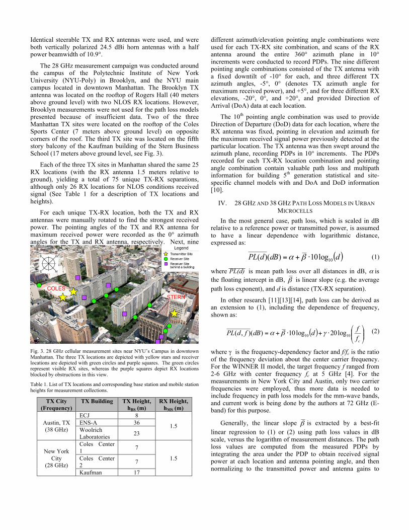
The 28 GHz measurement campaign was conducted around the campus of the Polytechnic Institute of New York University (NYU-Poly) in Brooklyn, and the NYU main campus located in downtown Manhattan. The Brooklyn TX antenna was located on the rooftop of Rogers Hall (40 meters above ground level) with two NLOS RX locations. However, Brooklyn measurements were not used for the path loss models presented because of insufficient data. Two of the three Manhattan TX sites were located on the rooftop of the Coles Sports Center (7 meters above ground level) on opposite corners of the roof. The third TX site was located on the fifth story balcony of the Kaufman building of the Stern Business School (17 meters above ground level, see Fig. 3).

Each of the three TX sites in Manhattan shared the same 25 RX locations (with the RX antenna 1.5 meters relative to ground), yielding a total of 75 unique TX-RX separations, although only 26 RX locations for NLOS conditions received signal (See Table 1 for a description of TX locations and heights).

For each unique TX-RX location, both the TX and RX antennas were manually rotated to find the strongest received power. The pointing angles of the TX and RX antenna for maximum received power were recorded as the 0° azimuth angles for the TX and RX antenna, respectively. Next, nine

Fig. 3. 28 GHz cellular measurement sites near NYU’s Campus in downtown Manhattan. The three TX locations are depicted with yellow stars and receiver locations are depicted with green circles and purple squares. The green circles represent visible RX sites, whereas the purple squares depict RX locations blocked by obstructions in this view. Table 1. List of TX locations and corresponding base station and mobile station heights for measurement collections.

TX City (Frequency)

TX Building TX Height,  hBS (m)

RX Height, hMS (m)

Austin, TX (38 GHz)

ECJ 8

1.5 ENS-A 36 Woolrich Laboratories 23

New York City

(28 GHz)

Coles Center 1 7

1.5 Coles Center 2 7

Kaufman 17

different azimuth/elevation pointing angle combinations were used for each TX-RX site combination, and scans of the RX antenna around the entire 360° azimuth plane in 10° increments were conducted to record PDPs. The nine different pointing angle combinations consisted of the TX antenna with a fixed downtilt of -10° for each, and three different TX azimuth angles, -5°, 0° (denotes TX azimuth angle for maximum received power), and +5°, and for three different RX elevations, -20°, 0°, and +20°, and provided Direction of Arrival (DoA) data at each location.

The 10th pointing angle combination was used to provide Direction of Departure (DoD) data for each location, where the RX antenna was fixed, pointing in elevation and azimuth for the maximum received signal power previously detected at the particular location. The TX antenna was then swept around the azimuth plane, recording PDPs in 10° increments. The PDPs recorded for each TX-RX location combination and pointing angle combination contain valuable path loss and multipath information for building 5th generation statistical and site-specific channel models with and DoA and DoD information [10].

IV. 28 GHZ AND 38 GHZ PATH LOSS MODELS IN URBAN MICROCELLS

In the most general case, path loss, which is scaled in dB relative to a reference power or transmitted power, is assumed to have a linear dependence with logarithmic distance, expressed as:

( )ddBdPL 10log10)()( ⋅+= βα (1)

where PL(d)¯¯¯¯¯ is mean path loss over all distances in dB, α is the floating intercept in dB, β is linear slope (e.g. the average path loss exponent), and d is distance (TX-RX separation).

In other research [11][13][14], path loss can be derived as an extension to (1), including the dependence of frequency, shown as:

( ) ⎟⎟⎠

⎞⎜⎜⎝

⎛⋅+⋅+=

cffddBfdPL 1010 log20log10)(),( γβα (2)

where γ is the frequency-dependency factor and f/fc is the ratio of the frequency deviation about the center carrier frequency. For the WINNER II model, the target frequency f ranged from 2-6 GHz with center frequency fc at 5 GHz [4]. For the measurements in New York City and Austin, only two carrier frequencies were employed, thus more data is needed to include frequency in path loss models for the mm-wave bands, and current work is being done by the authors at 72 GHz (E-band) for this purpose.

Generally, the linear slope β is extracted by a best-fit linear regression to (1) or (2) using path loss values in dB scale, versus the logarithm of measurement distances. The path loss values are computed from the measured PDPs by integrating the area under the PDP to obtain received signal power at each location and antenna pointing angle, and then normalizing to the transmitted power and antenna gains to

obtain channel path loss at each location and at each antenna pointing combination.

The estimate approach employed is the least-square linear regression fit, in which the linear slope β can be derived by [15]:

( ) ( )

( )∑∑

−

−×−=

n

i i

n

i ii

dd

PLPLdd2β (3)

where di is the distance in dB scale of the ith measurement PDP for a given antenna pointing angle and RX location, d is the average distance in dB of all di

in dB from the measurement snapshot, PLi is the path loss value of the ith measurement snapshot in dB and PL is the average path loss of the entire data set in dB, respectively.

The constant α in dB is the floating intercept of the linear regression fit in (1) that fits the data empirically, and can be thought of as a globally optimum reference attenuation set point that determines the tilt of the path loss model (1), and is found as [15]:

)(log10)()( 10 ddBPLdB ⋅−= βα (4)

For the linear regression fit, the values α and β are solved simultaneously in (3) and (4). The regression fit to obtain the best-fit values of α and β with minimum standard deviation has been done for all of the different system configurations listed in Table 2. Empirical path loss plots and regression line fits for path loss are shown in Figs. 4,5,6.

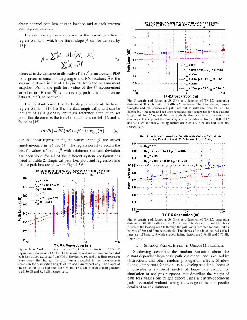
Fig. 4. New York City path losses at 28 GHz as a function of TX-RX separation distance at 28 GHz. The blue circles and red crosses are recorded path loss values extracted from PDPs. The dashed red and blue lines represent least-square fits through the path losses recorded in the measurement campaign for base station heights of 7m and 17m respectively. The slopes of the red and blue dashed lines are 3.73 and 4.51, while shadow fading factors are 8.36 dB and 8.54 dB, respectively.

Fig. 5. Austin path losses at 38 GHz as a function of TX-RX separation distance at 38 GHz with 13.3 dBi RX antennas. The blue circles, purple triangles and red crosses are path loss values extracted from PDPs. The dashed blue, magenta and red lines represent least-square fits for base stations heights of 8m, 23m, and 36m respectively from the Austin measurement campaign. The slopes of the blue, magenta and red dashed lines are 0.40, 0.12 and 0.41 while shadow fading factors are 8.23 dB, 5.78 dB and 5.96 dB, respectively.

Fig. 6. Austin path losses at 38 GHz as a function of TX-RX separation distance at 38 GHz with 25 dBi RX antennas. The dashed red and blue lines represent the least-square fits through the path losses recorded for base station heights of 8m and 36m respectively. The slopes of the blue and red dashed lines are 1.28 and 0.45 while shadow fading factors are 7.59 dB and 6.77 dB, respectively.

I. SHADOW FADING EFFECT IN URBAN MICROCELLS Shadowing describes the random variation about the

distant-dependent large-scale path loss model, and is caused by obstructions and other random propagation effects. Shadow fading is important for engineers to develop standards, because it provides a statistical model of large-scale fading for simulation or analysis purposes, that describes the ranges of path loss values one might expect using a distant-dependent path loss model, without having knowledge of the site-specific details of an environment.

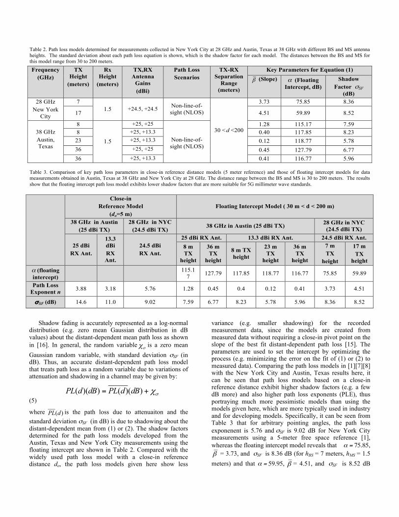
Table 2. Path loss models determined for measurements collected in New York City at 28 GHz and Austin, Texas at 38 GHz with different BS and MS antenna heights. The standard deviation about each path loss equation is shown, which is the shadow factor for each model. The distances between the BS and MS for this model range from 30 to 200 meters.

Table 3. Comparison of key path loss parameters in close-in reference distance models (5 meter reference) and those of floating intercept models for data measurements obtained in Austin, Texas at 38 GHz and New York City at 28 GHz. The distance range between the BS and MS is 30 to 200 meters. The results show that the floating intercept path loss model exhibits lower shadow factors that are more suitable for 5G millimeter wave standards.

Shadow fading is accurately represented as a log-normal distribution (e.g. zero mean Gaussian distribution in dB values) about the distant-dependent mean path loss as shown in [16]. In general, the random variable χσ is a zero mean Gaussian random variable, with standard deviation σSF (in dB). Thus, an accurate distant-dependent path loss model that treats path loss as a random variable due to variations of attenuation and shadowing in a channel may be given by:

σχ+= )()())(( dBdPLdBdPL (5)

where )(dPL is the path loss due to attenuaiton and the standard deviation σSF (in dB) is due to shadowing about the distant-dependent mean from (1) or (2). The shadow factors determined for the path loss models developed from the Austin, Texas and New York City measurements using the floating intercept are shown in Table 2. Compared with the widely used path loss model with a close-in reference distance do, the path loss models given here show less

variance (e.g. smaller shadowing) for the recorded measurement data, since the models are created from measured data without requiring a close-in pivot point on the slope of the best fit distant-dependent path loss [15]. The parameters are used to set the intercept by optimizing the process (e.g. minimizing the error on the fit of (1) or (2) to measured data). Comparing the path loss models in [1][7][8] with the New York City and Austin, Texas results here, it can be seen that path loss models based on a close-in reference distance exhibit higher shadow factors (e.g. a few dB more) and also higher path loss exponents (PLE), thus portraying much more pessimistic models than using the models given here, which are more typically used in industry and for developing models. Specifically, it can be seen from Table 3 that for arbitrary pointing angles, the path loss exponenent is 5.76 and σSF is 9.02 dB for New York City measurements using a 5-meter free space reference [1], whereas the floating intercept model reveals that α = 75.85, β = 3.73, and σSF is 8.36 dB (for hBS = 7 meters, hMS = 1.5 meters) and that α = 59.95, β = 4.51, and σSF is 8.52 dB

Frequency (GHz)

TX Height

(meters)

Rx Height

(meters)

TX,RX Antenna

Gains (dBi)

Path Loss Scenarios

TX-RX Separation

Range (meters)

Key Parameters for Equation (1)

β (Slope) α (Floating Intercept, dB)

Shadow Factor σSF

(dB) 28 GHz

New York City

7 1.5 +24.5, +24.5 Non-line-of-

sight (NLOS)

30 <d <200

3.73 75.85 8.36

17 4.51 59.89 8.52

38 GHz Austin, Texas

8

1.5

+25, +25

Non-line-of-sight (NLOS)

1.28 115.17 7.59 8 +25, +13.3 0.40 117.85 8.23

23 +25, +13.3 0.12 118.77 5.78 36 +25, +25 0.45 127.79 6.77 36 +25, +13.3 0.41 116.77 5.96

Close-in Reference Model

(do=5 m) Floating Intercept Model ( 30 m < d < 200 m)

38 GHz in Austin (25 dBi TX)

28 GHz in NYC (24.5 dBi TX)

38 GHz in Austin (25 dBi TX) 28 GHz in NYC (24.5 dBi TX)

25 dBi RX Ant.

13.3 dBi RX Ant.

24.5 dBi RX Ant.

25 dBi RX Ant. 13.3 dBi RX Ant. 24.5 dBi RX Ant. 8 m TX

height

36 m TX

height

8 m TX height

23 m TX

height

36 m TX

height

7 m TX

height

17 m TX

height α (floating intercept) 115.1

7 127.79 117.85 118.77 116.77 75.85 59.89

Path Loss Exponent n 3.88 3.18 5.76 1.28 0.45 0.4 0.12 0.41 3.73 4.51

σSF (dB) 14.6 11.0 9.02 7.59 6.77 8.23 5.78 5.96 8.36 8.52

(for hBS = 17 meters, hMS = 1.5 meters) for the identical measurement data set. Similarly in Austin, Texas, it can be seen that for the work in [7][8], the path loss exponent ranges from 3.18 to 3.88 and σSF ranges from 11 dB to 14.6 dB, whereas the floating intercept model reveals that α ranges from approximately 115 dB to 119 dB, β ranges from 0.12 to 1.28, and σSF ranges from about 6 dB to 8 dB for the identical measurement data set. Thus, it is apparent that the path loss models with close-in reference to free space show comparably higher PLEs and shadow factors than those presented in this paper. Note that the Austin, Texas measurement data set was much smaller than the New York City data set, and was recorded in a much less scatter-rich environment than New York City, which contributed to the lower path loss exponent values computed for Austin, Texas in Table 3. The results show that the new path loss model parameters given in Table 3, suggest that mmWave channels in urban environments will suffer less path loss than originally published in [1][7][8].

II. CONCLUSION Two measurement campaigns have been conducted in

urban microcellular environments in both New York City and Austin, Texas at 28 GHz and 38 GHz, respectively. The measurements were performed with a state-of-the-art sliding correlator channel sounder at 28 GHz and 38 GHz, and with a temporal resolution of 2.3 ns. Multiple possible microcellular communication scenarios were considered and investigated, using directional steerable antennas with various heights and gains. Linear regression fits, similar to those used in cellular standard bodies, have been used to create path loss models based on recorded path loss values that account for distance dependence. The shadow factors in our models here show a favorable advantage compared to widely used path loss models with close-in reference in academic research. Specifically, our models show that the shadow factor reduces approximately 1 dB in New York City and 6 dB in Austin, Texas. The model in this paper allows future realistic modeling of propagation conditions for millimeter wave transmission in urban microcellular environments. This model also suggests that in future millimeter wave communications, mobile devices shall deploy antennas with higher gains to compensate for the additional path loss due to the frequency leap from low microwave to the millimeter wave regime.

ACKNOWLEDGEMENT This work was sponsored by Samsung DMC R&D Communications Research Team (CRT), Intel, the National Science Foundation (NSF), and the GAANN Fellowship Program. The authors wish to thank Mathew Samimi, Yuanpeng Liu and Dr. Sundeep Rangan of NYU WIRELESS, UT-Austin administration, UT-Austin Public Safety, the NYU administration, NYU Public Safety, and NYPD for their contribution to this project. The measurements in Austin, Texas were taken under FCC Experimental License 0548-EX-PL-2010. The measurements in NYC were taken under U.S. FCC Experimental License 0040-EX-ML-2012.

REFERENCES [1] Y. Azar, G. N. Wong, K. Wang, R. Mayzus, J. K. Schulz, H. Zhao, F.

Gutierrez, D. Hwang, and T. S. Rappaport, “28 GHz Propagation Measurements for Outdoor Cellular Communications Using Steerable Beam Antennas in New York City,” 2013 IEEE International Conference on Communications (2013 ICC), June 9–13 2013.

[2] T.S. Rappaport, et.al, “Millimeter Wave Mobile Communications for 5G Cellular: It will work!” IEEE Access Journal, pp. 335-349, Vol. 1., No. 1, May 10, 2013.

[3] T. S. Rappaport, J. N. Murdock, and F. Gutierrez, “State of the Art in 60-GHz Integrated Circuits and Systems for Wireless Communications,” Proceedings of the IEEE, vol. 99, no. 8, pp. 1390–1436, August 2011.

[4] D. S. Baum, J. Salo, G. Del Galdo, M. Milojevic, P. Kyösti, and J. Hansen, “An interim channel model for beyond-3G systems,” in Proc. IEEE VTC’05, Stockholm, Sweden, May 2005.

[5] IST-WINNER D1.1.2 P. Kyösti, et al., "WINNER II Channel Models", ver 1.1, Sept. 2007. Available: https://www.ist-winner.org/WINNER2

[6] International Telecommunication Union Report ITU-R M. 2135-1, Guidelines for Evaluation of Radio Interface Technologies for IMT-Advanced, Dec. 2009.

[7] T.S. Rappaport, F. Gutierrez, Jr., E. Ben-Dor, J N. Murdock, Y. Qiao, J. I. Tamir, “Broadband Millimeter-Wave Propagation Measurements and Models Using Adaptive-Beam Antennas for Outdoor Urban Cellular Communications”, IEEE Transactions on Antennas and Propagations, Vol .61, No.4, April 2013.

[8] E. Ben-Dor, T.S. Rappaport, Y. Qiao, S.J. Lauffenburger, “Millimeter-wave 60 GHz Outdoor and Vehicle AOA Propagation Measurements using a Broadband Channel Sounder,” IEEE Global Telecommunications Conference (GLOBECOM 2011), Houston, TX, USA, 5–9 Dec. 2011.

[9] T. S. Rappaport, E. Ben-Dor, and J. N. Murdock, “38 GHz and 60 GHz Angle Dependent Propagation for Cellular and Peer to Peer Wireless Communications,” IEEE International Conference on Communications (2012 ICC), June 10–15 2012.

[10] M. Samimi, K. Wang, Y. Azar, G.N. Wong, R. Mayzus, H. Zhao, J.K. Schulz, S. Shu, F. Gutierrez, Jr. and T.S. Rappaport, “28 GHz Angle of Arrival and Angle of Departure Analysis for Outdoor Cellular Communications using Steerable Beam Antennas in New York City,” 2013 IEEE Vehicular Technology Conference (VTC), June 2–5, 2013.

[11] S. Piersanti, L. Annoni and D. Cassioli, “Millimeter Waves Channel Measurements and Path Loss Models,” IEEE International Conference on Communications (2012 ICC), June 10–15 2012.

[12] S. Shu, T.S. Rappaport, “Mulit-beam Antena Combining for 28 GHz Cellular Link Improvement in Urban Environments,” IEEE 2013 Global Communications Conference, to be published, Dec. 9–13, 2013.

[13] J. Keignart, “U.C.A.N. Report on UWB Basic Transmission Loss.” Tech. Rep. IST-2001-32710 U.C.A.N., Mar. 2003.

[14] A. Armogida et al., “Path-Loss Modelling in Short-Range UWB Transmissions,” in Intern. Workshop on Ultra Wideband Systems, Jun. 2003.

[15] J.F. Kenney, E.S. Keeping, “Mathematics of Statisitcs, Pt. 1,” 3rd ed., Princeton, NJ, 1962.

[16] T.S. Rappaport, “Wireless Communications: Principles and Practice”, 2nd ed.: Prentice Hall, 2002.