Ch232 lec21 jan2015

CH 232 : COMPUTATIONAL CHEMISTRY

INPUT AND OUTPUT

INPUT AND OUTPUT

COMPLEX

• Complex values may be edited under the control of pairs of F, E, EN, ES edit descriptors. The

two descriptors do not need to be identical. The complex value (0.1, 100.) converted under the

control of F6.1,E8.1 would be appear as

bbb0.1b0.1E+03.

where b stands for blank space.

• The two descriptors may be separated by character string and control edit descriptors.

LOGICAL

• Logical values may be edited using the LW edit descriptor.

• This defines a field of width w which on input consists of optional blanks, optionally followed by

a decimal point, followed by T or F (case insensitive), optionally followed by additional

characters.

• Thus a field defined by L7 permits the strings .true. and .false. to be input.

• The characters t or f will be transferred as the values true or false respectively.

• On output, the character T or F will appear in the right-most position in the output field.

INPUT AND OUTPUT

• In the previous examples, we saw that we can print out a character string by placing it inside

quotation marks inside the WRITE statement:

WRITE (*,*) ‘PLEASE ENTER X, Y, Z :’

• All we need to do to get the same effect with a FORMAT statement is to move the character

string inside the parentheses as a descriptor.

• EXAMPLE 8: Strings which are placed inside single apostrophes in the FORMAT statement are

printed intact:

WRITE (*, 21)

21 FORMAT (‘ ’, ‘PLEASE ENTER X, Y, Z :’)

This will result the following output:

• For this trivial example, moving the string inside the FORMAT statement is no improvement

over the list directed example. However, if we combine numerical data output with strings, we

can combine descriptive text with numerical data to improve comprehension.

• Example in the following page

INPUT AND OUTPUT

• EXAMPLE 9:

X = 12.34

Y = -0.025

WRITE (*, 34) X, Y, X*Y

34FORMAT (‘ ’, ‘X = ‘, F6.2, ‘ Y = ‘, F6.3, ‘ PROD = ‘, F10.5)

will produce the following output:

Let us examine the descriptors within the FORMAT statement:

‘ ’ Carriage Control Character – begin new line

‘X = ‘ Character string – Print X =

F6.2 Floating point format – Print out first number as XXX.XX

‘ Y = ‘ Character string – Print Y =

F6.3 Floating point format – Print out second number as XX.XXX

‘ PROD = ‘ Character string – Print PROD =

F10.5 Floating point format – Print out third number as XXXX.XXXXX

• Note that a blank space inside the apostrophes produces a blank space in the output. Thus,

‘ Y = ‘ produces [blank]Y[blank] =[blank] on the output line.

INPUT AND OUTPUT

• Formatting of character variables in a way similar to that for integers, where the only thing we

need to consider about is the total number of reserved spaces. The general form of the

FORMAT specifier is:

A w

where, A = indicates character format

w = total width of field reserved for character constant

• Characters can be of any length. This distinguishes them from numerical data, which have a

constant length (7 significant digits for reals for instance)

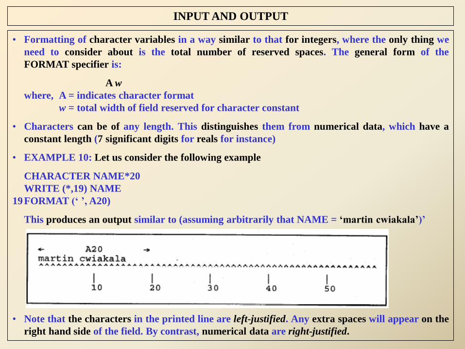
• EXAMPLE 10: Let us consider the following example

CHARACTER NAME*20

WRITE (*,19) NAME

19FORMAT (‘ ’,A20)

This produces an output similar to (assuming arbitrarily that NAME = ‘martin cwiakala’)’

• Note that the characters in the printed line are left-justified. Any extra spaces will appear on the

right hand side of the field. By contrast, numerical data are right-justified.

INPUT AND OUTPUT

• Character data is also different from numerical data in that it is not possible to overflow a field

with characters. If the field is too small for numerical data, a string of asterisk will appear. But

if the field is too small for character data, it simply truncates the extra characters.

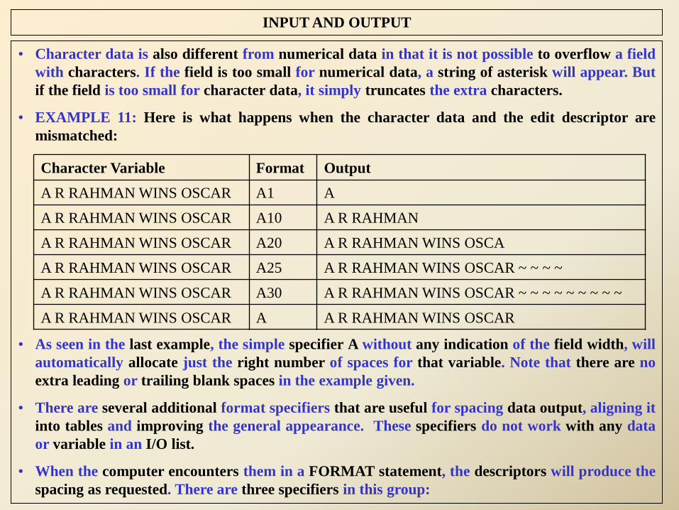
• EXAMPLE 11: Here is what happens when the character data and the edit descriptor are

mismatched:

• As seen in the last example, the simple specifier A without any indication of the field width, will

automatically allocate just the right number of spaces for that variable. Note that there are no

extra leading or trailing blank spaces in the example given.

• There are several additional format specifiers that are useful for spacing data output, aligning it

into tables and improving the general appearance. These specifiers do not work with any data

or variable in an I/O list.

• When the computer encounters them in a FORMAT statement, the descriptors will produce the

spacing as requested. There are three specifiers in this group:

Character Variable Format Output

A R RAHMAN WINS OSCAR A1 A

A R RAHMAN WINS OSCAR A10 A R RAHMAN

A R RAHMAN WINS OSCAR A20 A R RAHMAN WINS OSCA

A R RAHMAN WINS OSCAR A25 A R RAHMAN WINS OSCAR ~ ~ ~ ~

A R RAHMAN WINS OSCAR A30 A R RAHMAN WINS OSCAR ~ ~ ~ ~ ~ ~ ~ ~ ~

A R RAHMAN WINS OSCAR A A R RAHMAN WINS OSCAR

INPUT AND OUTPUT

• EXAMPLE 12: The spacing edit descriptors are easy to use and are very effective in improving

the appearance of our output. An example containing all three are given below: Let us assume,

BASE = 12.4, HEIGHT = 9.6 and VOL = 119.04.

WRITE (*, 9) BASE, HEIGHT, VOL

9 FORMAT (‘ ’, 5X, F9.3, /, 3X, ‘ X’, T7, F9.3, /,

$ T6, ‘________’, /, T7, F9.3)

will produce the following output

• APPEAR to be a complex example!!! (descriptions for each specifier are given in the following

page)

Descriptor General Form Example Function

X nX 3X Skip n spaces (3 spaces in the example)

/ / / Skip to next line

T Tn T32 Tab to column n (32 in this example)

INPUT AND OUTPUT

‘ ’ Carriage Control Character – begin new line (line 1)

5X Spacing command – skip 5 spaces (line 1)

F9.3 Floating point format – Print out first number as XXXXX.XXX

/ Spacing command – begin new line (line 2)

3X Spacing command – skip 3 spaces (line 2)

‘ X’ Character string – print X preceded by a blank space (line 2)

T7 Spacing command – tab to column 7 (line 2)

F9.3 Floating point format – Print out second number as XXXXX.XXX



‘________’ Character string – print ________ (line 3)



F9.3 Floating point format – Print out third number as XXXXX.XXX

• There is one additional form of the T specifier that we see occasionally. This form tells the

computer to move left or right a certain number of spaces from its current position. These are:

TRn (move right n spaces from current position)

TLn (move left n spaces from current position)

INPUT AND OUTPUT

• Note that these two commands depend on the current position within a line, while the Tn

command is independent of the line position (hence we have to be careful while using these

commands since they can “overwrite” what has been printed before.)

• REPEAT DESCRIPTOR

• There are many times when we need to reuse the same descriptor. A common situation is where

all the data are of same type and are to be printed out with the same format.

WRITE(*, 47) A, B, C, D, E, F, G, H

47FORMAT(‘ ’, F9.5, F9.5, F9.5, F9.5, F9.5, F9.5, F9.5, F9.5)

• As we can see, all eight variables are to printed with the same F9.5 format. Fortunately, Fortran

offers a shortcut to avoid repetitious use of a descriptor. All we need to do is to place a Repeat

Descriptor in front of the format to be repeated and then above FORMAT statement can be

rewritten as

WRITE(*, 47) A, B, C, D, E, F, G, H

47FORMAT(‘ ’, 8F9.5)

• This form of the Repeat Descriptor can be used with the I, F, F, D, G, and A formats. It cannot

be used in this form with the / descriptor.

• There is another form of the repeat descriptor where more complex combinations can be

repeated. Let us consider the following example:

WRITE(*, 47) A, B, C, D, E

47FORMAT(‘ ’, F9.5, 3X, F9.5, 3X, F9.5, 3X, F9.5, 3X, F9.5)

INPUT AND OUTPUT

• Note that there is a unit consisting of (F9.5, 3X) which repeats 5 times. The Repeat Descriptor

for this kind of instructions consists of an integer value representing the number of times

something is to be repeated and a set of parenthesis containing the repeat unit:

WRITE(*, 47) A, B, C, D, E

47FORMAT(‘ ’, 5(F9.5, 3X))

• The only exception to the above rules is the ‘/’ descriptor. The ‘/’ mark indicates that we are

finished with the current line and we want the next bit of output on the following line. If we wish

to skip three lines, the following are equivalent:

/, /, /, / or //// or 4(/)

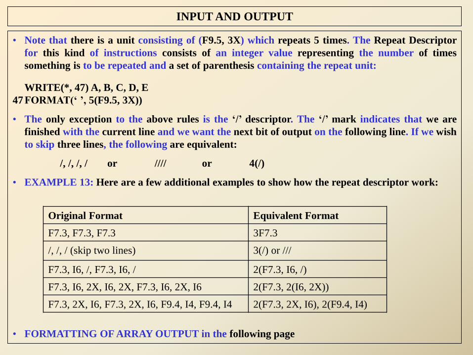
• EXAMPLE 13: Here are a few additional examples to show how the repeat descriptor work:

• FORMATTING OF ARRAY OUTPUT in the following page

Original Format Equivalent Format

F7.3, F7.3, F7.3 3F7.3

/, /, / (skip two lines) 3(/) or ///

F7.3, I6, /, F7.3, I6, / 2(F7.3, I6, /)

F7.3, I6, 2X, I6, 2X, F7.3, I6, 2X, I6 2(F7.3, 2(I6, 2X))

F7.3, 2X, I6, F7.3, 2X, I6, F9.4, I4, F9.4, I4 2(F7.3, 2X, I6), 2(F9.4, I4)

INPUT AND OUTPUT

• EXAMPLE 14: For the following example, A is a one dimensional array of 10 elements and B is

a 3 3 two-dimensional integer array. The value assigned to each element is:

A

B

• Below are examples of how the output would appear for a variety of formatted implied DO

loops:

1 2 3 4 5 6 7 8 9 10

1 2 3

4 5 6

7 8 9

Program Segment Output

a) WRITE (*, 10) (A(I), I = 1, 5)

10 FORMAT (‘ ’, 5(F4.1, 1X)) 1.0 2.0 3.0 4.0 5.0

b) WRITE (*, 10) (A(I), I = 1, 5)

10 FORMAT (‘ ’, 20(F4.1, 1X)) 1.0 2.0 3.0 4.0 5.0

c) WRITE (*, 10) (A(I), I = 1, 10)

10 FORMAT (‘ ’, 5(F4.1, 1X))

1.0 2.0 3.0 4.0 5.0

6.0 7.0 8.0 9.0 10.0

d) WRITE (*, 10) ((B(I,J), J = 1, 3), I = 1, 3)

10 FORMAT (‘ B:’, 3(/, 1X, 3(F4.1, 1X)))

B:

1.0 2.0 3.0

4.0 5.0 6.0

7.0 8.0 9.0

INPUT AND OUTPUT

Program Segment Output

e) WRITE (*, 10) ((B(I,J), J = 1, 3), I = 1, 3)

10 FORMAT (‘ ’, 3(F4.1, 1X))

1.0 2.0 3.0

4.0 5.0 6.0

7.0 8.0 9.0

f) N= 3

DO 20 I = 1, N

WRITE (*, 10) (B(I,J), J = 1, N)

10 FORMAT (‘ ’, 100(F4.1, 1X))

20 CONTINUE

1.0 2.0 3.0

4.0 5.0 6.0

7.0 8.0 9.0

• \

• In the example a), the FORMAT statement, 5(F4.1, 1X) repeats the descriptors “F4.1, 1X” five times.

• Example b) illustrates what happens if there are more formatting instructions than actually needed. The

result is that the unused formatting is simply ignored.

• Example c) illustrates an insufficient number of edit descriptors. In this case output is printed until all the

formatting instructions are used. Then the output continues on a new line and the format instructions are

reused. Hence, the results in printing two rows of five columns each.

• Example d) illustrates the use of the repeat specifiers and the end-of-line descriptor (/). When using the end-

of-line descriptor to generate the output on a new line, we will have to include a CCC. Most often, this is most

conveniently done with the 1X edit descriptor.

• Example e) illustrates how to take advantage of that fact that when formatting runs out, the computer repeats

the edit descriptors on a new line. This allows for a simple format statement to print out a two-dimensional

array. The only drawback of this approach is that we must know the size in advance, and we cannot change it

without changing our FORMAT statement.

• Example f) illustrates this combining explicit and implicit DO loops.

INPUT AND OUTPUT

• Although FORMAT statements can be used with either READ or WRITE

statements, they are used for controlling output. The reason is that if we use

FORMATs with a READ statement, the data must be entered exactly as

spelled out in the FORMAT statement.

• If we type too many or too few zeros or spaces, the data will be read

incorrectly. Therefore, it is recommended that we avoid formatted READ

statements.

• The exception is when we want to read data from a data file, which we will

be discussing shortly. In some situations like this, we usually have no choice

but to use formatted READs.

• Another point to remember is that when a FORMAT statement is used with

a READ statement, there is no carriage control Character. These are limited

to output on a printer.

PARAMETER AND DATA STATEMENTS

• THE PARAMETER STATEMENT

• The PARAMETER statement is an EASY way of creating named constants.

• Named constants have elements of both constants and variables. On the one hand they are

constants whose value cannot change under any circumstances, and on the other hand they are

given names like a variable.

• A good example is PI. Once we assign a value to the named constant PI with the PARAMETER

statement, its value cannot change. Any attempt to change a named constant results in an error

during compilation.

• One of the most common uses of the named constant is to declare arrays whose size is likely to

change. The advantage of this approach is that we can make many changes throughout the

program by making a single change in the named constant.

• The general form of the PARAMETER statement is:

PARAMETER (variable1 = value, variable2 = value . . .)

• Each named constant is given its value inside the parentheses following the PARAMETER key

word. Once a name is specified here, it cannot be used as a conventional variable within the

program, and its value cannot be reassigned by an assignment statement, function, or READ

statement.

• EXAMPLE in the following page


• EXAMPLE: Here is an example of a PARAMETER statement that allows us to declare several arrays

simultaneously. Let us a consider a program which process 100 data points with the following array

declarations (without the PARAMETER STATEMENT)

REAL VOLTS(100), I(100), IMPED(100), RESIST(100)

INTEGER TIME(100), COUNTS(100), SIZE(100)

• Now, if we wish to change the program for 1000 data points, then we will have to change each array dimension

from 100 to 1000 (tedious!!!).

• An easier way to is to use the PARAMETER statement when we first set up a program to define a named

constant such as N below:

PARAMETER (N = 100)

REAL VOLTS(N), I(N), IMPED(N), RESIST(N)

INTEGER TIME(N), COUNTS(N), SIZE(N)

• When we want to increase the size of the arrays, we need only change a single PARAMETER statement. This

method is useful for changing values those are scattered through out the program (Example is given below)

PARAMETER (N = 100)

REAL VOLTS(N), I(N), IMPED(N), RESIST(N)

INTEGER TIME(N), COUNTS(N), SIZE(N)

…

READ (*,*) (VOLTS(K) = 1, N)

…

DO 10 L = 1, N

10 CONTINUE

…

WRITE (*,*) (IMPED(M), M = 1, N)

STOP

END


• THE DATA STATEMENT

• The DATA statement is used to assign initial values to a variable.

• Whereas the PARAMETER statement assigns permanent values, the DATA statement assigns

temporary values.

• DATA statements are most useful to replace READ statements at the beginning of a program

and save the trouble of having repetitive data every time we run a program.

• The general form of the DATA statement is:

DATA object-list / value-list/

where object-list is a list of variables and implied – do loops; and value –list is a list of scalar

constants and structure constructors.

• The list of variables after the DATA statement can include either single-valued variables and

arrays. Values to be assigned to these variables are contained within the slash (/) marks and will

be assigned to the corresponding variable by virtue of its position within the list.

• After any array or array section in object-list has been expanded into a sequence of scalar

elements in array element order, there must be as many constants in each value-list as scalar

elements in the corresponding object-list. Each scalar element is assigned the corresponding

scalar constant.

• If arrays are specified within the DATA variable list, we may use an implied DO loop, just as we

do with the input statements:


DATA (array(subscript), subscript = start, stop, step) /value1, value2, . . . /

The implied DO loop will specify the array elements to receive the values listed inside the

slashes.

• EXAMPLE:

a) One common area where we use DATA statements is to assign initial values to a list of single-

valued variables:

Without DATA Statements:

VOLTS = 5.3

RESIST = 1000.0

CAPICT = 0.000035

With DATA Statements:

DATA VOLTS, RESIST, CAPICT /5.3, 1000.0, 0.000035/

b) Quite often when we use DATA statements, several of the variables may receive the same value.

In this case, we have a shorthand notation

Long Way: DATA A, B, C, D, E, F /1.0, 1.0, 1.0, 1.0, 1.0, 1.0/

Short Way: DATA A, B, C, D, E, F /6*1.0/

The star (*) here does not imply multiplication. Instead, it indicates that the number which

follows is to be repeated the indicated number of times.


c) DATA statements are particularly useful when initializing arrays:

REAL A(100)

DATA (A(I), I = 1, 100) /50*0.0, 50*1.0/

These statements assign 0.0 to the first 50 elements of A, and 1.0 to the last 50 elements.

d) The implied DO loop may not be necessary if all elements are to be assigned. Here is a shorter

way of writing example c):

REAL A(100)

DATA A /50*0.0, 50*1.0/

If the array is a two-dimensional array, the data values will be assigned by columns if we use

this simple form:

REAL B(3, 3)

DATA A /1.0, 2.0, 3.0, 4.0, 5.0, 6.0, 7.0, 8.0, 9.0/

This will result in the following assignments B:

e) If we wish to assign the data by rows instead of columns, then we will have to use the full

implied DO loop:

REAL A(10, 10)

DATA ((A(I, J), J = 1, 10), I = 1, 10) /50*10.0, 50*100.0/

The first five rows are filled with 10.0’s and the remaining five are filled with 100.0’s. If the

implied DO loops were not present, then this array would have been filled differently (the first

five columns would have 10.0’s and the remaining columns would have 100.0’s)

1 2 3

4 5 6

7 8 9


• In the examples given so far, the types and type parameters of the constants in a value-list have

always been the same as the type of the variables in the object-list.

• This need not be the case, but they must be compatible for intrinsic assignment since the entity

is initialized following the rules for intrinsic assignment.

• It is thus possible to write statements such as

Data q /54/, i /3.1/ … where q is real, i is integer

• Integer values may be binary, octal, or hexadecimal constants

• Each variable must either have been typed in a previous type declaration statement in the

scoping unit, or its type is that associated with the first letter of its name according to the

implicit typing rules of the scoping unit.

• In the case of implicit typing, the appearance of the name of the variable in a subsequent type

declaration statement in the scoping unit must confirm the type and type parameters.

• Similarly, any array variable must have previously been declared as such.

• No variable or part of a variable may be initialized more than once in a scoping unit.

CH 232 : COMPUTATIONAL CHEMISTRY

DATA FILES

DATA FILES

• Up to now, we have done all input and output through the keyboard and the terminal screen

(CRT/LCD/TFT). While this is convenient, there is no permanent record of the program results.

As soon as the CRT/LCD/TFT screen is cleared, all output is lost.

• Figure 1 illustrates the direct write of data to the CRT/LCD/TFT screen

DATA FILES

• There are many times, however, it would be desirable to send data to a file so that another

program or user could access this information later.

• Figure 2 illustrates the writing to a data file

DATA FILES

• It is sometimes desirable to be able to read data from a file rather than to enter them from the

keyboard. A good example is when we are writing a program that requires a large amount of

input data.

• Let us assume that our program require 100 data points and that we have set it up without the

use of an input file. Whenever we rerun the program, we must re-enter the data by hand. So if

we needed to edit the program 10 times before we removed all the bugs, we would have entered

a total of 1000 data points by hand !!!.

• However, if we read the data from a data file, only once is required to enter the data (or an even

better scheme has the computer itself generate the data and enter it into a file for us)

• Data files are no different from other type of files, such as the one in which we store our

program. These files may be manipulated with commands from the operating system. For

example, we can type them onto our CRT/LCD/TFT screen, send them onto printer(s), or make

duplicate copies of the data on another disk.

• One of the biggest advantages of data files is that we can access within our program. Thus, we

can send our output to an alternate output device instead of the CRT/LCD/TFT.

• Mostly, data will be sent to a data file. Other options might be a printer, floppy, pen drive, or

hard disks, FAX modem, plotters, CD disks, and so forth.

• Here we will be focusing on the technique for diverting I/O from within a program to a device

other than the CRT/LCD/TFT. To do this, we have to include following things in our program:

• Instructions to open a file

• Instructions to communicate with the designated file

• Instructions to close the file when finished

DATA FILES

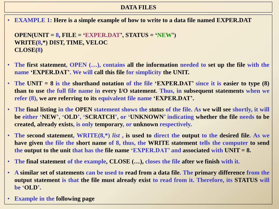
• EXAMPLE 1: Here is a simple example of how to write to a data file named EXPER.DAT

OPEN(UNIT = 8, FILE = ‘EXPER.DAT’, STATUS = ‘NEW’)

WRITE(8,*) DIST, TIME, VELOC

CLOSE(8)

• The first statement, OPEN (…), contains all the information needed to set up the file with the

name ‘EXPER.DAT’. We will call this file for simplicity the UNIT.

• The UNIT = 8 is the shorthand notation of the file ‘EXPER.DAT’ since it is easier to type (8)

than to use the full file name in every I/O statement. Thus, in subsequent statements when we

refer (8), we are referring to its equivalent file name ‘EXPER.DAT’.

• The final listing in the OPEN statement shows the status of the file. As we will see shortly, it will

be either ‘NEW’, ‘OLD’, ‘SCRATCH’, or ‘UNKNOWN’ indicating whether the file needs to be

created, already exists, is only temporary, or unknown respectively.

• The second statement, WRITE(8,*) list , is used to direct the output to the desired file. As we

have given the file the short name of 8, thus, the WRITE statement tells the computer to send

the output to the unit that has the file name ‘EXPER.DAT’ and associated with UNIT = 8.

• The final statement of the example, CLOSE (…), closes the file after we finish with it.

• A similar set of statements can be used to read from a data file. The primary difference from the

output statement is that the file must already exist to read from it. Therefore, its STATUS will

be ‘OLD’.

• Example in the following page

DATA FILES

• EXAMPLE 2: In the following example, we will read data from a file named ‘NOBEL.DAT’ and

assign the data to the variables WEIGHT, MASS, and DENSIT. Notice that the file must already

exist in order to read from it.

OPEN(UNIT = 3, FILE = ‘NOBEL.DAT’, STATUS = ‘OLD’)

READ(3,*) WEIGHT, MASS, DENSIT

CLOSE(3)

• Notice that the READ statement goes to unit #3, which is the shorthand notation for the file

‘NOBEL.DAT’.

• Also note that the status of the file is ‘OLD’, which indicates that it is a valid file for reading. If

the status had not been ‘OLD’, a syntax error would have been resulted.

• In Fortran Terminology, a file is said to exist in the restricted sense that it exists as a file to

which the program might have access.

• In other words, if the program is prohibited from using the file because of a password

protection system, or because some necessary action has not been taken in the job control

language which is controlling the execution of the program, the file ‘doesn’t exist’.

• A file which exists for a running program may be empty and may or may not be connected to

that program. The file is connected if it is associated with a unit number known to the program.

• Such connection is usually made by executing an open statement for the file, but many computer

systems will pre-connect certain files which any program may be expected to use, such as

terminal input and output. Thus we see that a file may exist but not be connected.

Ch232 lec21 jan2015

Documents

Transcript of Ch232 lec21 jan2015