A&A 493, 1197–1222 (2009)DOI: 10.1051/0004-6361:200810426c© ESO 2009

Astronomy&

Astrophysics

CARS: the CFHTLS-Archive-Research Survey

I. Five-band multi-colour data from 37 sq. deg. CFHTLS-wide observations�

T. Erben1, H. Hildebrandt2,1, M. Lerchster3,4, P. Hudelot1,6, J. Benjamin5, L. van Waerbeke5, T. Schrabback2,1,F. Brimioulle3, O. Cordes1, J. P. Dietrich7, K. Holhjem1, M. Schirmer1, and P. Schneider1

1 Argelander-Institut für Astronomie, University of Bonn, Auf dem Hügel 71, 53121 Bonn, Germanye-mail: terben@astro.uni-bonn.de

2 Sterrewacht Leiden, Leiden University, Niels Bohrweg 2, 2333 CA Leiden, The Netherlands3 University Observatory Munich, Department of Physics, Ludwigs-Maximillians University Munich, Scheinerstr. 1, 81679 Munich,

Germany4 Max-Planck-Institut für extraterrestrische Physik, Giessenbachstraße, 85748 Garching, Germany5 Department of Physics and Astronomy, University of British Columbia, Vancouver, BC V6T 1Z1, Canada6 Institut d’Astrophysique de Paris, 98bis bd. Arago, 75014 Paris, France7 ESO, Karl-Schwarzschild-Strasse 2, 85748 Garching, Germany

Received 19 June 2008 / Accepted 7 November 2008

ABSTRACT

Context. We present the CFHTLS-Archive-Research Survey (CARS). It is a virtual multi-colour survey that is based on public archiveimages from the Deep and Wide components of the CFHT-Legacy-Survey (CFHTLS). Our main scientific interests in the CFHTLSWide-part of CARS are optical searches for galaxy clusters from low to high redshift and their subsequent study with photometric andweak-gravitational lensing techniques.Aims. As a first step in the CARS project, we present multi-colour catalogues from 37 sq. degrees of the CFHTLS-Wide component.Our aims are first to create astrometrically and photometrically well-calibrated co-added images from publicly available CFHTLSdata. Second, we offer five-band (u∗g′r′i′z′) multi-band catalogues with an emphasis on reliable estimates for object colours. Theseare subsequently used for photometric redshift estimates.Methods. We consider all those CFHTLS-Wide survey pointings that were publicly available on January 2008 and that also have five-band coverage in u∗g′r′i′z′. The data were calibrated and processed with our GaBoDS/THELI image processing pipeline. The qualityof the resulting images was thoroughly checked against the Sloan-Digital-Sky Survey (SDSS) and already public high-end CFHTLSdata products. From the co-added images we extracted source catalogues and determined photometric redshifts using the publiccode Bayesian Photometric Redshifts (BPZ). Fifteen of our survey fields directly overlap with public spectra from the VIMOSVLT deep (VVDS), DEEP2 and SDSS redshift surveys, which we used for calibration and verification of our redshift estimates.Furthermore we applied a novel technique, based on studies of the angular galaxy cross-correlation function, to quantify the reliabilityof photo-z’s.Results. With this paper we present 37 sq. degrees of homogeneous and high-quality five-colour photometric data from the CFHTLS-Wide survey. The median seeing of our data is better than 0.′′9 in all bands and our catalogues reach a 5σ limiting magnitude ofabout i′AB ≈ 24.5. Comparisons with the SDSS indicate that most of our survey fields are photometrically calibrated to an accuracy of0.04 mag or better. This allows us to derive photometric redshifts of homogeneous quality over the whole survey area. The accuracyof our high-confidence photo-z sample (10−15 galaxies per sq. arcmin) is estimated with external spectroscopic data to σΔz/(1+z) ≈0.04−0.05 up to i′AB < 24 with typically only 1−3% outliers. In the spirit of the Legacy Survey we make our catalogues available tothe astronomical community. Our products consist of multi-colour catalogues and supplementary information, such as image masksand JPEG files to visually inspect our catalogues. Interested users can obtain the data by request to the authors.

Key words. surveys – galaxies: photometry

1. Introduction

Being the signposts of the largest density peaks of the cosmicmatter distribution, clusters of galaxies are of particular inter-est for cosmology. The statistical distribution of clusters as a

� Based on observations obtained with MegaPrime/MegaCam, a jointproject of CFHT and CEA/DAPNIA, at the Canada-France-HawaiiTelescope (CFHT), which is operated by the National Research Council(NRC) of Canada, the Institut National des Sciences de l’Univers ofthe Centre National de la Recherche Scientifique (CNRS) of France,and the University of Hawaii. This work is based in part on dataproducts produced at TERAPIX and the Canadian Astronomy DataCentre (CADC) as part of the Canada-France-Hawaii Telescope LegacySurvey, a collaborative project of NRC and CNRS.

function of mass and redshift forms one of the key cosmologicalprobes. Since their dynamical or evolutionary timescale is notmuch shorter than the Hubble time, they contain a “memory”of the initial conditions for structure formation (e.g. Borgani& Guzzo 2001). The population of clusters evolves with red-shift, and this evolution depends on the cosmological model(e.g. Eke et al. 1996). Therefore, the redshift dependence ofthe cluster abundance has been used as a cosmological test(e.g. Bahcall & Fan 1998; Borgani et al. 1999; Schuecker et al.2003a,b). A prerequisite for these studies are large and homoge-neous cluster samples with well-understood selection functions.Consequently, a wide variety of systematic searches have beenperformed in various parts of the electromagnetic spectrum. Themost extensive cluster searches and cosmological studies were

Article published by EDP Sciences

1198 T. Erben et al.: CARS – Five-band multi-colour data from 37 sq. deg. archival CFHTLS observations

performed in X-rays (see e.g. Böhringer et al. 2000; Reiprich &Böhringer 2002; Böhringer et al. 2004; Mantz et al. 2008) andin the optical (see e.g. Postman et al. 1996; Olsen et al. 1999;Gladders & Yee 2000; Goto et al. 2002; Bahcall et al. 2003;Gladders et al. 2007; Koester et al. 2007); see also Gal (2008)for a concise review of various cluster detection algorithms inthe optical. Each of the cluster searches relies on certain clusterproperties such as X-ray emission of the hot intra-cluster gas oran optical overdensity of red galaxies and may introduce system-atic biases in the candidate list creation. Hence, a careful com-parison and selection with different methods on the same area ofthe sky is essential to obtain a comprehensive understanding ofgalaxy clusters and their mass properties.

The Wide part of the Canada-France-Hawaii-TelescopeLegacy Survey (CFHTLS-Wide) is an optical Wide-Field-Imaging-Survey particularly well suited for such studies. Whencompleted it will cover 170 sq. deg. in the five optical Sloanfilters u∗g′r′i′z′ to a limiting magnitude of i′AB ≈ 24.5. Theunique combination of area, depth and wavelength coverage al-lows the application of a variety of currently available opti-cal search algorithms. For instance, the Postman matched fil-ter technique (see Postman et al. 1996) applies an overdensityand luminosity function filter to photometric data of a singleband survey. It can provide high-confidence samples in the low-and medium redshift range (see e.g. Olsen et al. 1999, 2001).The Red-Cluster-Sequence algorithm scans a two-filter surveyfor the Red Sequence of elliptical galaxies and is mainly usedfor the medium to high redshift regime with the r and z fil-ters (Gladders & Yee 2000). The existence of five bands in theCFHTLS-Wide allows us to estimate photometric redshifts andthe application of techniques using distance information (e.g.Miller et al. 2005). Furthermore, one of the main goals of theCFHTLS-Wide are weak gravitational lensing studies of thelarge-scale structure distribution (see e.g. Hoekstra et al. 2006;Fu et al. 2008, for recent results). This will allow us to comple-ment and to directly compare optical cluster searches with candi-dates from weak lensing mass reconstructions and shear peak de-tections (see e.g. Schneider 1996; Erben et al. 2000; Bartelmann& Schneider 2001; Wittman et al. 2001; 2003; Dahle et al. 2003;Hetterscheidt et al. 2005; Wittman et al. 2006; Schirmer et al.2007; Dietrich et al. 2007). To perform these galaxy clusterstudies, we perform an extensive Archive-Research programmeon publicly available data from the CFHTLS-Wide. We baptiseour survey the CFHTLS-Archive-Research Survey (CARS in thefollowing).

This paper marks the first step of our science programmeon a significant area of CARS. We describe our data handlingand the creation of multi-colour catalogues, including a firstset of photometric redshifts, on 37 sq. degrees of five-colourCARS data.

The article is organised as follows: Sect. 2 gives a shortoverview on our current data set; a detailed description ofour complete image data handling is given in Appendix A.Sections 3 and 4 summarise the multi-colour catalogue creationand the photometric redshift estimation together with a thoroughquantification of their quality. We continue to describe our dataproducts (Sect. 5) and finish with our conclusions in Sect. 6.

2. The data

The current set of CARS data consists of a subset of the syn-optic CFHTLS-Wide observations which is one of three inde-pendent parts of the Canada-French-Hawaii-Telescope LegacySurvey (CFHTLS). It is a very large, 5-year project designed

and executed jointly by the Canadian and French communities.The survey started in spring 2003 and is planned to finish dur-ing 2008. All observations are carried out with the MegaPrimeinstrument mounted at the Canada-France-Hawaii Telescope(CFHT). MegaPrime (see e.g. Boulade et al. 2003) is an op-tical multi-chip instrument with a 9 × 4 CCD array (2048 ×4096 pixel in each CCD; 0.′′186 pixel scale; ≈1◦ × 1◦ totalfield-of-view). When completed, the CFHTLS-Wide will cover170 sq. deg. in four high-galactic-latitude patches W1�W4 of 25 to72 square degrees through the five optical filters u∗g′r′i′z′ downto a magnitude of i′AB ≈ 24.5. See http://www.cfht.hawaii.edu/Science/CFHLS/ and http://terapix.iap.fr/cplt/oldSite/Descart/summarycfhtlswide.html for further in-formation on survey goals and survey implementation.

Since June 2006 CFHTLS observations are publicly releasedto the astronomical community via the Canadian AstronomyData Centre (CADC)1. At the time of writing raw and Elixirpreprocessed images (see below), together with auxiliary meta-data, can be obtained 13 months after observations.

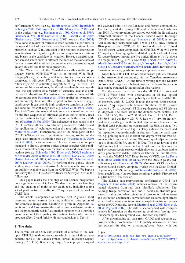
For the current work we consider all Elixir processedCFHTLS-Wide fields with observations in all five opticalcolours u∗g′r′i′z′ which were publicly available on 18/01/2008,i.e. observed until 18/12/2006. In total, the current CARS set con-sists of 37 sq. degrees split between the three CFHTLS-Widepatches W1 (21 sq. degrees), W3 (five sq. degrees) and W4 (elevensq. degrees). The areas around the defined patch centres (W1:RA = 02:18:00, Dec = −07:00:00, W3: RA = 14:17:54, Dec =+54:30:31 and W4: RA = 22:13:18, Dec = +01:19:00) are cov-ered on a regular grid with pointed observations. Names of in-dividual CARS pointings are constructed like W1m1p2 (read “W1minus 1 plus 2′′; see also Fig. 1). They indicate the patch andthe separation (approximately in degrees) from the patch cen-tre, e.g. pointing W1m1p2 is about one degree west and two de-grees north from the W1 centre. The overlap of adjacent point-ings is about 3.′0 in RA and 6.′0 in Dec. The exact layout of theCARS survey fields is shown in Fig. 1. All three patches are cov-ered by spectroscopic surveys which allow us to calibrate and toverify photometric redshift estimates later on; W1 and W4 over-lap with the VIMOS VLT Deep Survey (VVDS; see Le Fèvreet al. 2005; Garilli et al. 2008), W3 with the DEEP2 galaxy red-shift survey (see Davis et al. 2007). Moreover, CARS data frompatches W3 and W4 have complete overlap with the Sloan-Digital-Sky-Survey (SDSS; see e.g. Adelman-McCarthy et al. 2007).From patch W1 only the southern pointings W1p3m0, W1p4m0 andW1p1m1 have SDSS overlap.

The Elixir data preprocessing performed at CFHT (seeMagnier & Cuillandre 2004) includes removal of the instru-mental signature from raw data (bias/dark subtraction; flat-fielding; fringe correction in i′ and z′ data) and absolute pho-tometric calibration (determination of zeropoints, colour termsand extinction coefficients, corrections for scattered light effectswhich lead to significant inhomogeneous photometric zeropointsacross the CCD mosaic, see e.g. Manfroid et al. 2001; Koch et al.2004; Regnault 2007). The data is accompanied with compre-hensive information on the observing conditions (seeing, sky-transparency, sky-background level) for each exposure2.

After downloading all data from CADC and rejecting ex-posures with a problematic CFHT quality assessment we fur-ther process the data on a pointing/colour basis with our

1 Seehttp://www1.cadc-ccda.hia-iha.nrc-cnrc.gc.ca/cadc/2 See http://www.cfht.hawaii.edu/Science/CFHTLS-DATA/exposurescatalogs.html

T. Erben et al.: CARS – Five-band multi-colour data from 37 sq. deg. archival CFHTLS observations 1199

W1m0p1

W1m0p2

W1m0p3

W1m1p1

W1m1p2

W1m1p3

W1p1m1

W1p1p1

W1p1p2

W1p1p3

W1p2p1

W1p2p2

W1p2p3

W1p3m0

W1p3p1

W1p3p2

W1p3p3

W1p4m0

W1p4p1

W1p4p2

W1p4p3

W4m0m0

W4m0m1

W4m0m2

W4m1m1

W4m1m2

W4p1m0

W4p1m1

W4p1m2

W4p2m0

W4p2m1

W4p2m2

Fig. 1. Layouts of the current three CARS: the CARS data of this work are split up in the three CFHTLS-Wide patches W1 (21 sq. degrees; patchcentre: RA = 02:18:00, Dec = −07:00:00), W3 (five sq. degrees; patch centre: RA = 14:17:54, Dec = +54:30:31) and W4 (11 sq. degrees; patchcentre: RA = 22:13:18, Dec = +01:19:00). In areas covered by thick lines spectra from various surveys are publicly available for photo-z calibrationand verification (see text for details).

GaBoDS/THELI pipeline to produce deep co-added images forscientific exploitation. Our algorithms and software modules toprocess multi-chip cameras are described in Erben et al. (2005)and most of the details do not need to be repeated here. For theinterested reader we give in Appendix A a thorough descriptionof the CARS data handling, data peculiarities and the pipeline up-grades/extensions necessary to smoothly and automatically pro-cess MegaPrime data. In addition, a comprehensive assessmentof the astrometric and photometric quality of our data, togetherwith a comparison to previous releases of CFHTLS data can befound there. We conclude that the CARS data set is accuratelyastrometrically and photometrically calibrated for multi-colourphotometric and lensing studies.

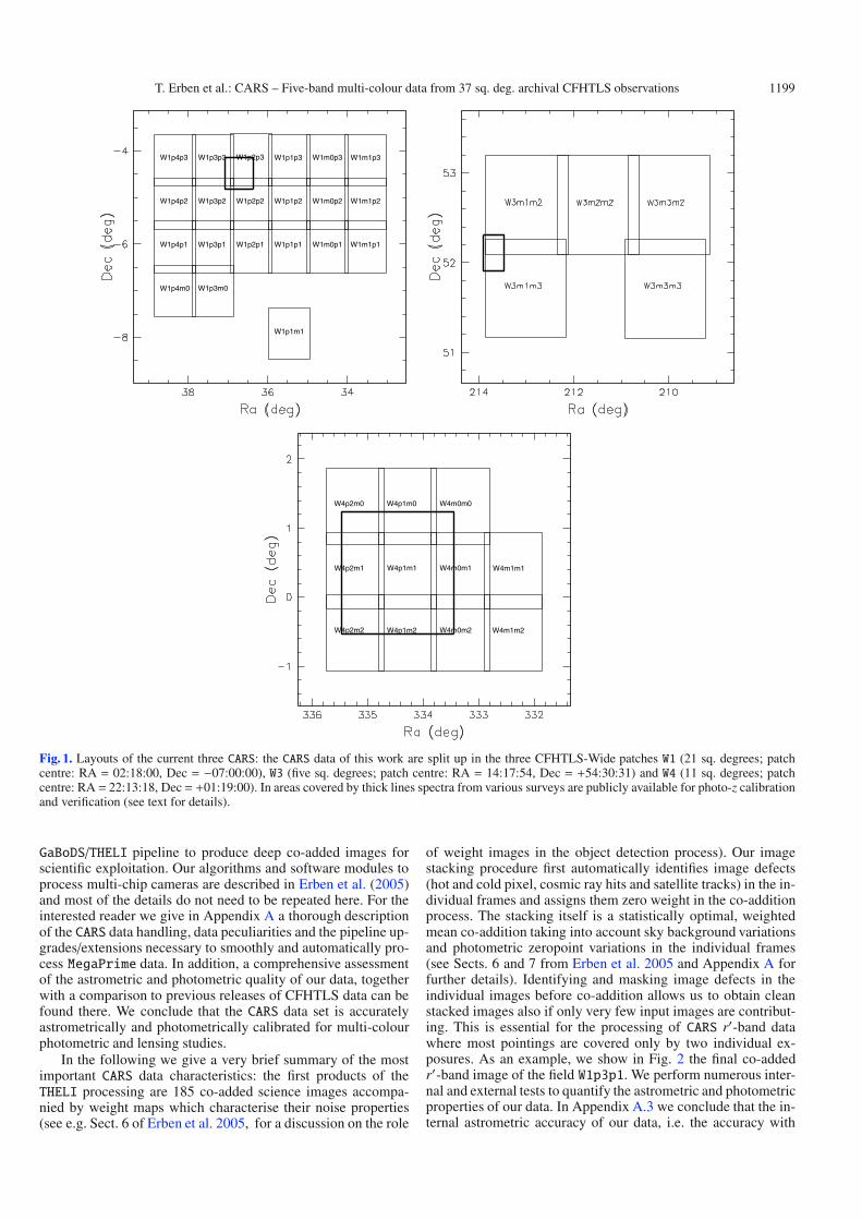
In the following we give a very brief summary of the mostimportant CARS data characteristics: the first products of theTHELI processing are 185 co-added science images accompa-nied by weight maps which characterise their noise properties(see e.g. Sect. 6 of Erben et al. 2005, for a discussion on the role

of weight images in the object detection process). Our imagestacking procedure first automatically identifies image defects(hot and cold pixel, cosmic ray hits and satellite tracks) in the in-dividual frames and assigns them zero weight in the co-additionprocess. The stacking itself is a statistically optimal, weightedmean co-addition taking into account sky background variationsand photometric zeropoint variations in the individual frames(see Sects. 6 and 7 from Erben et al. 2005 and Appendix A forfurther details). Identifying and masking image defects in theindividual images before co-addition allows us to obtain cleanstacked images also if only very few input images are contribut-ing. This is essential for the processing of CARS r′-band datawhere most pointings are covered only by two individual ex-posures. As an example, we show in Fig. 2 the final co-addedr′-band image of the field W1p3p1. We perform numerous inter-nal and external tests to quantify the astrometric and photometricproperties of our data. In Appendix A.3 we conclude that the in-ternal astrometric accuracy of our data, i.e. the accuracy with

1200 T. Erben et al.: CARS – Five-band multi-colour data from 37 sq. deg. archival CFHTLS observations

Fig. 2. Co-added CARS data: We show the final science image of the r′-band observations from field W1p3p1 (left panel) and the accompanyingweight map (right panel). The weight map shows five extended satellite tracks which were automatically identified and masked before imageco-addition (see Appendix A.2 for details). In several CARS pointings/colours individual chips did not contain useful data and were hence excludedfrom the analysis. The pointing shown suffered from this problem in the uppermost row.

which we can align individual exposures of a colour and point-ing, is 0.′′03−0.′′04 (1/5th of a MegaPrime pixel) over the wholefield-of-view of MegaPrime; our absolute astrometric frame isgiven by the USNO-B1 catalogue (see Monet et al. 2003). Theco-added images of the different colours from each pointing arealigned to sub-pixel precision in all cases.

We quantify the quality of the photometric calibration ofour data in Appendices A.4, A.6 and A.7. First, we investigatephotometric flatness over the MegaPrime field-of-view. We usedata from the CFHTLS-Deep survey which keeps observing foursq. degrees over the whole five-year period of the CFHT-LegacySurvey. This allows us to create image stacks from differentepochs and to investigate photometric consistency. Magnitudecomparisons of co-additions obtained from the three years 2003,2004 and 2005 indicate uniform photometric properties with adispersion of σint,u∗g′r′i′ ≈ 0.01−0.02 mag in u∗g′r′i′ and aboutσint,z′ ≈ 0.03−0.04 mag in z′. We attribute higher residuals in z′to fringe residuals in this band.

Our absolute magnitude zeropoints are tested against pho-tometry in the SDSS and against previous data releases of theCFHTLS. Our comparison with the SDSS shows that our ab-solute photometric calibration agrees with Sloan to σabs,g′r′i′ ≈0.01−0.04 mag in g′r′i′ and σabs,z′ ≈ 0.03−0.05 mag for z′.While the calibration in these four bands seems to be unbiased,we observe, at the current stage, a systematic magnitude offsetin u∗ of about 0.1 mag with respect to Sloan (CARS magnitudesappear fainter than Sloan). For u∗-band data from spring to fall2006 our analysis suggests an Elixir calibration problem lead-ing to offsets of 0.2−0.3 mag in u∗.

Finally, we directly compared our flux measurements withthose of the previous CFHTLS TERAPIX T0003 release andStephen Gwyn’s MegaPipe project (see Gwyn 2008). The mea-surements to T0003 are in very good agreement with typical dis-persions of 0.02 mag; in many cases larger scatters are observedwith respect to the MegaPipe data. Private communication withGwyn suggests that several MegaPipe stacks suffer from theaccidental inclusion of images obtained under unfavourable

Table 1. Characteristics of the CARS co-added science data with basicaverage properties of our final science data (see text for an explanationof the columns).

Filter expos. time [s] mlim [AB mag] seeing [′′]u∗(u.MP9301) 5 × 600 (3000) 25.24 0.87g′(g.MP9401) 5 × 500 (2500) 25.30 0.85r′(r.MP9601) 2 × 500 (1000) 24.36 0.79i′(i.MP9701) 7 × 615 (4305) 24.68 0.71z′(z.MP9801) 6 × 600 (3600) 23.20 0.66

photometric conditions; see Appendices A.7 and A.8 for furtherdetails.

Table 1 lists average properties for seeing and limiting mag-nitude values in our survey data. The quoted values for expo-sure time (we list the typical exposure time per dither, the num-ber of dithered observations per colour and the total exposuretime in parentheses), limiting magnitudes and seeing correspondto a typical field and hence give a good indication of what canbe expected from the data. The seeing values (SExtractor pa-rameter FWHM_IMAGE for stellar sources) are the median ofmeasured seeing values from all co-added science images in thecorresponding filters. We note that we measure a seeing of 1.′′0or below for all co-added CARS stacks except for the u∗-bandimage of W1p3p3 for which we obtain 1.′′1. The limiting magni-tude is defined as the 5-σ detection limit in a 2.′′0 aperture viamlim = ZP − 2.5 log (5

√Npixσsky), where ZP is the magnitude

zeropoint, Npix is the number of pixels in a circle with radius 2.′′0and σsky the sky background noise variation. The actual num-bers for mlim in Table 1 were obtained from the field W4p2m0. Itrepresents a CARS pointing with typical properties concerningexposure times and image seeing. A more detailed table list-ing these quantities for each individual field can be found inAppendix A.9.

The described imaging data form the basis for the subsequentmulti-colour catalogue creation and photo-z estimation.

T. Erben et al.: CARS – Five-band multi-colour data from 37 sq. deg. archival CFHTLS observations 1201

3. The multi-colour catalogues

Our procedures to create multi-colour catalogues for the five-band CARS data are similar to the ones presented in Hildebrandtet al. (2006) where we studied Lyman-break galaxies in the ESODeep Public Survey (DPS).

3.1. Preparation and PSF equalisation

In order to estimate unbiased colours it is necessary to measureobject fluxes in the same physical apertures in each band, i.e.for a given object the same physical parts of the object shouldbe measured in the different bands. Since the PSF usually variesfrom band to band we apply a convolution to degrade the see-ing of all images of one field to the PSF size of the image withthe worst seeing. Assuming a Gaussian PSF we first measurethe seeing and then calculate appropriate filter functions by thefollowing formula:

σfilter,k =

√σ2

worst − σ2k , (1)

with σfilter,k being the width of the Gaussian filter for convolutionof the kth image, σworst being the PSF size of the image with theworst seeing, and σk being the PSF size of the kth image. Bydoing so we neglect the non-Gaussianity of a typical ground-based PSF. Nevertheless, experience with the DPS shows thatour procedure is sufficient to estimate reliable colours if the see-ing values in the individual colours are subarcsecond and not toodifferent. In CARS, the seeing values for a pointing typically donot differ by more than 0.′′2−0.′′3 (see Table A.2).

3.2. Limiting magnitudes

The images filtered in that way are then analysed for their sky-background properties. For the accurate estimation of photomet-ric redshifts it is important to have a reasonable estimate for thelimiting magnitude at a given object position. Therefore, we cre-ate limiting magnitude maps from the rms fluctuations of thesky-background in small parts of the image. Here we use 1σ lim-iting magnitudes calculated in a circular aperture of 2× stellarFWHM diameter. This procedure ensures that varying depthsover the field are properly taken into account in the colour es-timation. It may well be that an object would be detected in onepart of the image whereas it is undetectable in a different partdue to the dither pattern or stray-light leading to inhomogeneousdepth. By assigning position-dependent limiting magnitudes toeach object in all bands we can later decide which flux measure-ments are significant and which are not.

3.3. Object detection

The object detection is performed with SExtractor (see Bertin& Arnouts 1996) in dual-image mode and we consider all ob-jects having at least 5 connected pixels exceeding 2σ of the sky-background variation. We will base our primary science analyses(galaxy cluster searches and weak lensing applications) on thei′-band data. Hence, we generate our object catalogues based onthis colour rather than on a combination of all available colourssuch as a χ2 image (see e.g. McCracken et al. 2003). We use theunconvolved i′-band image as the detection image and measurefluxes for the colour estimation and the photometric redshifts onthe convolved frames. Colour indices are estimated from the dif-ferences of isophotal magnitudes taking into account local lim-iting magnitudes, i.e. if a magnitude is measured to be fainter

than the local limiting magnitude, then this limit is used insteadof the measured magnitude to estimate an upper/lower bound forthe colour index.

Additionally, we also measure the total i′-band magnitudeson the unconvolved image so that total magnitudes in the otherbands can in principle be calculated from those and from thecolour indices. However, it should be noted that our approachto run SExtractor in dual-image-mode with the unconvolvedi′-band image for detection will never lead to accurate total mag-nitudes in the u∗g′r′z′-bands. While adding/subtracting the ap-propriate colour index to/from the total i′-band magnitude yieldsaccurate total magnitudes in one of the other bands for brightobjects without a colour gradient, it can yield strongly biasedresults in other cases. Only catalogues created in single-image-mode on the different bands assure a reliable estimation of totalmagnitudes. Since our emphasis here is on estimating colours asaccurately as possible, we do not pursue this issue further.

3.4. Creation of image masks

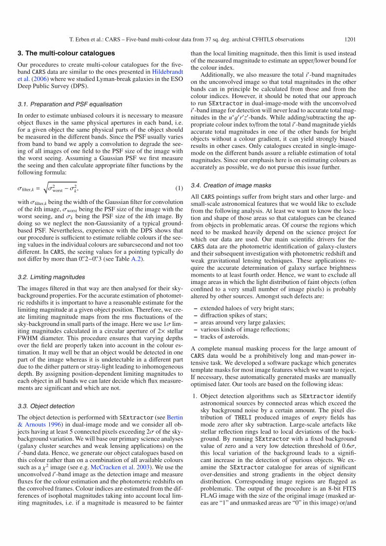
All CARS pointings suffer from bright stars and other large- andsmall-scale astronomical features that we would like to excludefrom the following analysis. At least we want to know the loca-tion and shape of those areas so that catalogues can be cleanedfrom objects in problematic areas. Of course the regions whichneed to be masked heavily depend on the science project forwhich our data are used. Our main scientific drivers for theCARS data are the photometric identification of galaxy-clustersand their subsequent investigation with photometric redshift andweak gravitational lensing techniques. These applications re-quire the accurate determination of galaxy surface brightnessmoments to at least fourth order. Hence, we want to exclude allimage areas in which the light distribution of faint objects (oftenconfined to a very small number of image pixels) is probablyaltered by other sources. Amongst such defects are:

– extended haloes of very bright stars;– diffraction spikes of stars;– areas around very large galaxies;– various kinds of image reflections;– tracks of asteroids.

A complete manual masking process for the large amount ofCARS data would be a prohibitively long and man-power in-tensive task. We developed a software package which generatestemplate masks for most image features which we want to reject.If necessary, these automatically generated masks are manuallyoptimised later. Our tools are based on the following ideas:

1. Object detection algorithms such as SExtractor identifyastronomical sources by connected areas which exceed thesky background noise by a certain amount. The pixel dis-tribution of THELI produced images of empty fields hasmode zero after sky subtraction. Large-scale artefacts likestellar reflection rings lead to local deviations of the back-ground. By running SExtractor with a fixed backgroundvalue of zero and a very low detection threshold of 0.6σ,this local variation of the background leads to a signifi-cant increase in the detection of spurious objects. We ex-amine the SExtractor catalogue for areas of significantover-densities and strong gradients in the object densitydistribution. Corresponding image regions are flagged asproblematic. The output of the procedure is an 8-bit FITSFLAG image with the size of the original image (masked ar-eas are “1” and unmasked areas are “0” in this image) or/and

1202 T. Erben et al.: CARS – Five-band multi-colour data from 37 sq. deg. archival CFHTLS observations

a saoimage/ds9 polygon region file of masked areas. SeeDietrich et al. (2007) for further details on the algorithm andits implementation.

2. Astronomical Standard Star Catalogues such as USNO-B1,GSC-2 or SDSS-R5 list the positions and magnitudes ofknown astronomical sources up to a magnitude of about 18.In the CARS data, the large majority of these objects withm ≤ 16 are bright or moderately bright stars whose surround-ings should be excluded from object catalogues (faint haloes,diffraction spikes). Moreover, stellar sources have well de-fined shapes over the complete MegaPrime field-of-view.The extent of the central light concentration and the widthand the height of stellar diffraction spikes can be modelledas function of apparent magnitude. On the basis of these ob-servations we automatically create object masks for stellarobjects:– We retrieve object positions and magnitudes from

the Standard Star Catalogues GSC-1, GSC-2.3.2 andUSNO-A2. We found that our selection criteria in thesecatalogues (magnitude limits, catalogue flags) result inslightly different source lists and hence the three sam-ples complement each other. Our masking is performedindependently on all three catalogues.

– At each catalogue position we lay down template masksfor the central light halo and the diffraction spikes. Thetemplates are scaled with (red photographic) magni-tude to conservatively encompass the stellar areas. Inaddition, for very bright stars with m < 10.35 wemask extended stellar diffraction haloes. For MegaPrimethese haloes have an extend of about 4.′0 dependingonly weakly on magnitude. Moreover, these haloes oc-cur with a radial offset towards the MegaPrime centre.The halo displacement from the stellar centre as func-tion of MegaPrime position can well be described by−0.022 times the relative position of the star with respectto the camera centre.

– Finally, the masks are converted to saoimage/ds9polygon region files which can further be processedby the WeightWatcher programme (see Bertin &Marmo 2007; Marmo & Bertin 2008) to construct aFLAG_IMAGE file.

3. Tracks of fast moving asteroids typically show up as a se-ries of high S/N, lined up, short dashed and highly ellipticalobjects in co-added CARS images. They are present in thedata because our strictly linear co-addition process does notinclude any pixel rejection/clipping procedure. We try to de-tect and mask them in our multi-colour object catalogues.We identify an asteroid candidate if a minimum number ofN objects are located within 0.4 pixels from a line connectingany two objects within overlapping boxes of M × M pixels2.We run this algorithm for the two parameter sets N = 4;M = 100 and N = 5; M = 175 and merge the resulting can-didate lists. This combination was found empirically to givegood results on the CARS data set. For real asteroids the el-lipticities of contributing objects are usually highly aligned.As in weak lensing theory (see e.g. Bartelmann & Schneider2001) we compute the two-component ellipticity

(ε1, ε2) =1 − r1 + r

(cos 2θ, sin 2θ) , (2)

which depends on the object axis ratio r and position an-gle θ as determined by SExtractor. The expectation valueof both ellipticity components is zero if the ellipticities of

different objects are not aligned. We then compute the align-ment estimator

A =√

[median(ε1)]2 + [median(ε2)]2 (3)

from the ellipticities of all objects belonging to a candidate.We only keep asteroid candidates with A > 0.20; A > 0.24(first and second parameter set) in order to minimise the falseflagging of galaxies in areas with increased object numberdensity, such as galaxy clusters. These parameters were opti-mised for typical CARS seeing conditions and image depths.For the W4m0m0 field the algorithm automatically masks30 out of 32 visually identified asteroid tracks, with one falsepositive, for an object number density of 35/arcmin2.

We note that the different algorithms are complementary to eachother. While large-scale features such as very large galaxies orimage borders influence the object density, small scale defectsfrom medium bright stars (diffraction spikes; outer extendedhaloes) are caught by masking known catalogue sources. We in-dependently run the object density analysis on all five colours ofa CARS pointing. However, the stellar and asteroid track masksare calculated for the i′-band only. The latter ones need somemanual revision which is done on the basis of the i′-band im-age only. Hence, asteroid tracks in the u∗g′r′z′ bands are not in-cluded in our object masks. Other problems which require man-ual optimisation of the image masks are: (1) the object densitydistribution analysis also masks rich galaxy clusters. (2) Someobjects labelled as stellar source in the Standard Star Cataloguesare galaxies. (3) For images with an exceptional good seeingof 0.′′6 or better the high density of objects leads to a signifi-cant number of false positives in the asteroid masking. The finalmasks from the individual colours are merged and collected inone saoimage/ds9 polygon region file. The masking informa-tion is also transferred to our multi-colour catalogues as a MASKkey which allows an easy filtering of problematic sources later.Figure 3 shows examples of our masking procedure.

4. Photometric redshifts

From the multi-colour catalogues described in the preceding sec-tion we estimate photometric redshifts for all objects in twosteps. In a first pass we use available spectroscopic informa-tion from the VVDS3 to correct/recalibrate our photometric ze-ropoints on a patch-wide basis. Afterwards we obtain photo-zestimates for our objects (see Hildebrandt et al. 2008). In thefollowing we set the minimal photometric error to 0.1 mag in or-der to avoid very small purely statistical errors for high-S/N ob-jects and to take into account our estimated internal and externalphotometric accuracies (see Sect. A.8). Throughout this workwe use MegaPrime filter response curves which were computedby Mathias Schultheis and Nicolas Regnault. They are avail-able at http://terapix.iap.fr/forum/showthread.php?tid=1364.

The following analysis only includes secure VVDS objects(marked by flags 3, 4, 23 and 24; in total these are 4463 ob-jects for W1 (up to a limiting magnitude of i′AB ≈ 24) and

3 Spectroscopic data were obtained from http://cencosw.oamp.fr/VVDS/4 Note that there are at least two more sets of MegaPrime filter curvesavailable on the WWW: On the CFHT web pages (http://www.cfht.hawaii.edu/Instruments/Filters/megaprime.html) andon Stephen Gwyn MegaPipe pages (http://www1.cadc-ccda.hia-iha.nrc-cnrc.gc.ca/megapipe/docs/filters.html)

T. Erben et al.: CARS – Five-band multi-colour data from 37 sq. deg. archival CFHTLS observations 1203

Fig. 3. Semi-automatic image masking: shown is the result of our semi-automatic image masking for areas of the field W4m0m0. The polygonsquares result from our object density analysis and the stars coversources identified in the GSC-1, GSC-2.3.2 and USNO-A2 StandardStar Catalogues (upper panel; multiple masks around stars appear forsources identified in various catalogues). The lower panel shows resultsfrom our asteroid masking procedure.

9617 for W4 (up to i′AB ≈ 22.5)). Here and in the followingwe match objects from our source lists with those from exter-nal catalogues if their position agrees to better than 1.′′0. Firstwe run the new version of Hyperz (Bolzonella et al. 2000)5

on 13 fields with overlap to the VVDS6, four of which are inW1 and nine in W4. We use the CWW template set (Colemanet al. 1980) supplied by Hyperz and add two starburst tem-plates from Kinney et al. (1996). Additionally, we fix the red-shift to the spectroscopic redshift for every object. In this waywe find the best fitting template at the spectroscopic redshiftfor every object. Hyperz puts out the magnitudes of the best-fittemplates and enables us to compare these to our original es-timates. We average the differences between the observed andthe best-fit template’s magnitudes over all objects. In this waywe derive corrections for the zeropoints in the five bands. Weonly use spectra of galaxies with i′AB ≤ 21.5 which have a highS/N photometric measurement in all filter bands; these were654 sources in W1 and 2158 objects in W4. The mean and the

5 Publicly available at http://www.ast.obs-mip.fr/users/roser/hyperz/6 Spectroscopic data were obtained from http://cencosw.oamp.fr/

scatter of the corrections in the four W1 fields areΔu∗ = −0.064±0.015 mag, Δg′ = 0.069 ± 0.005 mag, Δr′ = 0.027 ± 0.019 mag,Δi′ = −0.004 ± 0.018 mag, and Δz′ = 0.007 ± 0.007 mag. In thenine W4 fields we findΔu∗ = −0.088± 0.011 mag,Δg′ = 0.136±0.029 mag, Δr′ = 0.019 ± 0.03 mag, Δi′ = 0.008 ± 0.023 mag,and Δz′ = −0.010 ± 0.014 mag. Note that the photo-z code isonly sensitive to colours so that the absolute values of the cor-rections in the different bands should not be misunderstood aspure calibration errors. Prior to the calibration step, we did notmodify the W3 and W4 u∗ zeropoints for identified systematic cal-ibration problems (see Appendix A.4). As all W3 and W4 fieldsare equally affected by it we expect that it is taken into accountproperly by our correction procedure. We also did not apply anygalactic extinction corrections to our catalogues.

For the W1 fields that do not overlap with the VVDS we usethe zeropoint corrections from the field W1p2p3, the one withthe highest density of spectroscopic redshifts in the W1 region.Since the regions W3 and W4 show different u∗-band calibrationsystematics than W1 (see Sect. A.6), we correct all W3 fields andthe two W4 fields without VVDS overlap with the values fromW4p1m1, again the most densely covered field in this region.

Then we run Bayesian Photometric Redshifts (BPZ;see Benitez 2000)7 on the catalogues with the corrected pho-tometry using the same template set as before. The Bayesianapproach of BPZ combines spectral template χ2 minimisationwith a redshift/magnitude prior. The prior was calibrated fromHDF-N observations and the Canada-France Redshift Survey(see Lilly et al. 1995). It contains the probability of a galaxy hav-ing redshift z and spectral type T given its apparent magnitude m.A detailed description of the code and the prior can be found inBenitez (2000). We restrict the fitting of the photo-z’s to z ≤ 3.9due to the limited depth of the Wide data. The Bayesian redshiftestimates are added to our multi-colour catalogues. Note that notall objects in our catalogues have well determined photometricmeasurements in the full u∗ to z′ wavelength coverage. This canhave physical reasons (e.g. high-redshift dropout galaxies whichare fainter than the magnitude limit in blue passpands) or it canbe connected to problems in the data itself (e.g. pixels withoutinformation in one of the filter bands). Our current cataloguesmiss information to cleanly distinguish between these cases butonly allow us to identify problematic photometry by either largephotometric errors or a flux measurement below the formal de-tection limit. In all cases with a magnitude estimate below thelimiting magnitude, or a magnitude error larger than 1 mag, weconfigured BPZ to treat the object as non-detected with a flux er-ror equal to the 1σ limiting magnitude. This leads to unreliableresults if the large photometric error results e.g. from image de-fects and not from intrinsic source properties. To allow an easyrejection of such problematic sources each object in our cata-logues obtains photometry quality flags for all filter bands.

The internal accuracy of the BPZ photo-z’s is described bythe ODDS parameter (see e.g. Mobasher et al. 2004) assigninga probability to the Bayesian redshift estimate by integrating theposterior probability distribution in an interval that correspondsto the 95% confidence interval for a single-peaked Gaussian. Byrejecting the most unsecure objects with a low ODDS value onecan obtain much cleaner subsamples; see also Hildebrandt et al.(2008).

If not stated otherwise we use in quality assessments of ourBPZ photo-z’s the following subsample of our catalogue data:

1. we reject all objects falling within an object mask (seeSect. 3.4);

7 Publicly available at http://acs.pha.jhu.edu/~txitxo/

1204 T. Erben et al.: CARS – Five-band multi-colour data from 37 sq. deg. archival CFHTLS observations

Table 2. Statistics of the comparison between photometric and spectro-scopic VVDS redshifts.

Field mlim Na compl.b outl. rate ηc Δz/(1 + z)d

[AB] [%] [%]W1p2p2 22.5 212 91.51 1.03 0.000 ± 0.052

24.0 517 73.11 1.85 −0.002 ± 0.050W1p2p3 22.5 1136 92.52 0.86 −0.008 ± 0.051

24.0 2456 77.69 1.62 −0.011 ± 0.049W1p3p2 22.5 14 92.86 0.00 0.009 ± 0.040

24.0 24 70.83 0.00 0.011 ± 0.047W1p3p3 22.5 104 87.50 2.20 0.004 ± 0.046

24.0 257 65.37 1.79 0.009 ± 0.050W4m0m0 22.5 223 93.27 1.44 −0.015 ± 0.045W4m0m1 22.5 354 94.63 2.69 0.004 ± 0.049W4m0m2 22.5 132 98.48 0.77 −0.001 ± 0.048W4p1m0 22.5 395 92.91 0.82 0.006 ± 0.045W4p1m1 22.5 908 95.70 1.96 −0.010 ± 0.051W4p1m2 22.5 416 95.19 1.26 0.001 ± 0.051W4p2m0 22.5 274 94.89 0.77 −0.013 ± 0.045W4p2m1 22.5 517 96.52 1.00 −0.006 ± 0.051W4p2m2 22.5 263 94.30 0.40 −0.007 ± 0.050

a The number of uniquely matched sources between our cataloguesand high-confidence VVDS objects (see also text); b the percentageof sources from column three (N) with a high-confidence BPZ photo-z estimate (ODDS > 0.9); c defined as the percentage of galaxies with(zphot−zspec)/(1+zspec) > 0.15; d bias and scatter of (zphot−zspec)/(1+zspec)after outlier rejection.

2. we select galaxies by means of the SExtractor star-galaxy classifier CLASS_STAR and reject all sources withCLASS_STAR > 0.95;

3. we include only objects with reliable photometry in all fivefilter bands (see above);

4. finally we reject all sources with ODDS < 0.9.

Our catalogues contain in total 3.9 million galaxies outside anobject mask (rejection steps 1 and 2) and finally 1.45 millionsources (about 13 galaxies per sq. arcmin) with reliable BPZphoto-z estimates (object sample after all rejections).

We first compare our photo-z’s from W1 and W4 to spectro-scopic redshifts from the VVDS in a similar way as presentedin Hildebrandt et al. (2008). Note that these spectra were pre-viously used to calibrate the data! Table 2 summarises the re-sults indicating a homogeneous dispersionσΔz/(1+z) ≈ 0.04−0.05and an outlier rate (defined as the percentage of galaxies with(zphot − zspec)/(1 + zspec) > 0.15) of 1−2% up to i′AB = 24. TheσΔz/(1+z) statistics is estimated after outliers have been rejected.If we perform the spectro-z vs. photo-z comparisons with theODDS > 0.0 sample (but all other filters as described above) thedispersion is nearly unchanged while the outlier rate rises by afactor 3 to 8. This confirms that the ODDS parameter is a goodselection criterion to reject outliers and to obtain samples of ho-mogeneous photo-z quality up to about i′AB ≈ 24. A plot of thephoto-z vs. VVDS spectro-z results in the regions W1 and W4 isshown in Fig. 4. While the figure shows an overall good perfor-mance of our photo-z estimation it reveals residual systematics.A significant tilt is present in the zphot vs. zspec comparison lead-ing to a systematic overestimation of up to 0.1−0.2 of the red-shift at low zspec and to a underestimation at high zspec. The tiltcrosses the zero axis at z = 0.5 and hence it cancels negativeand positive contributions to statistics involving Δz (see Fig. 4).The Δz/(1 + z) statistics for the complete W1 (N = 1466) andW4 (N = 3488) samples are: Δz/(1 + z) = −0.006 ± 0.051 (W1)and Δz/(1 + z) = −0.005+/−0.050 (W4). If we split the sample

Fig. 4. Photometric vs. spectroscopic redshifts in the W1 and W4 re-gions: we show in the upper panels 1349 (W1) and 3312 (W4) galax-ies with i′AB < 22.5, reliable VVDS flags, good photometry in all fivefilter bands and ODDS > 0.9 (points). Triangles represent galaxieswith 0 < ODDS < 0.9 (117 sources in W1 and 170 objects in W4).Lower panels show a binned distribution of 〈zphot − zspec〉 from theODDS > 0.9 samples of the upper panels.

at z = 0.5 we obtain for z < 0.5: Δz/(1 + z) = 0.03 ± 0.043(W1: N = 595) and Δz/(1 + z) = 0.025 ± 0.037 (W4: N = 1690).Accordingly for 0.5 < z < 1.0: Δz/(1+ z) = −0.032 ± 0.035 (W1:N = 809) and Δz/(1 + z) = −0.034 ± 0.038 (W1: N = 1728).

We do not try to remedy these systematics in this article butwe will investigate it in a companion paper (Hildebrandt et al.,in prep.). The overestimation at the low-z is mainly caused by theredshift prior in BPZ. It seems to give too little probability to thelow-z population in the CARS data. A modification of the originalprior in this sense removes the observed bias for 0 < z < 0.5.The high-z underestimation of our redshifts can be corrected bya recalibration of the original Coleman et al. (1980) and Kinneyet al. (1996) template sets; see also Feldmann et al. (2006). In

T. Erben et al.: CARS – Five-band multi-colour data from 37 sq. deg. archival CFHTLS observations 1205

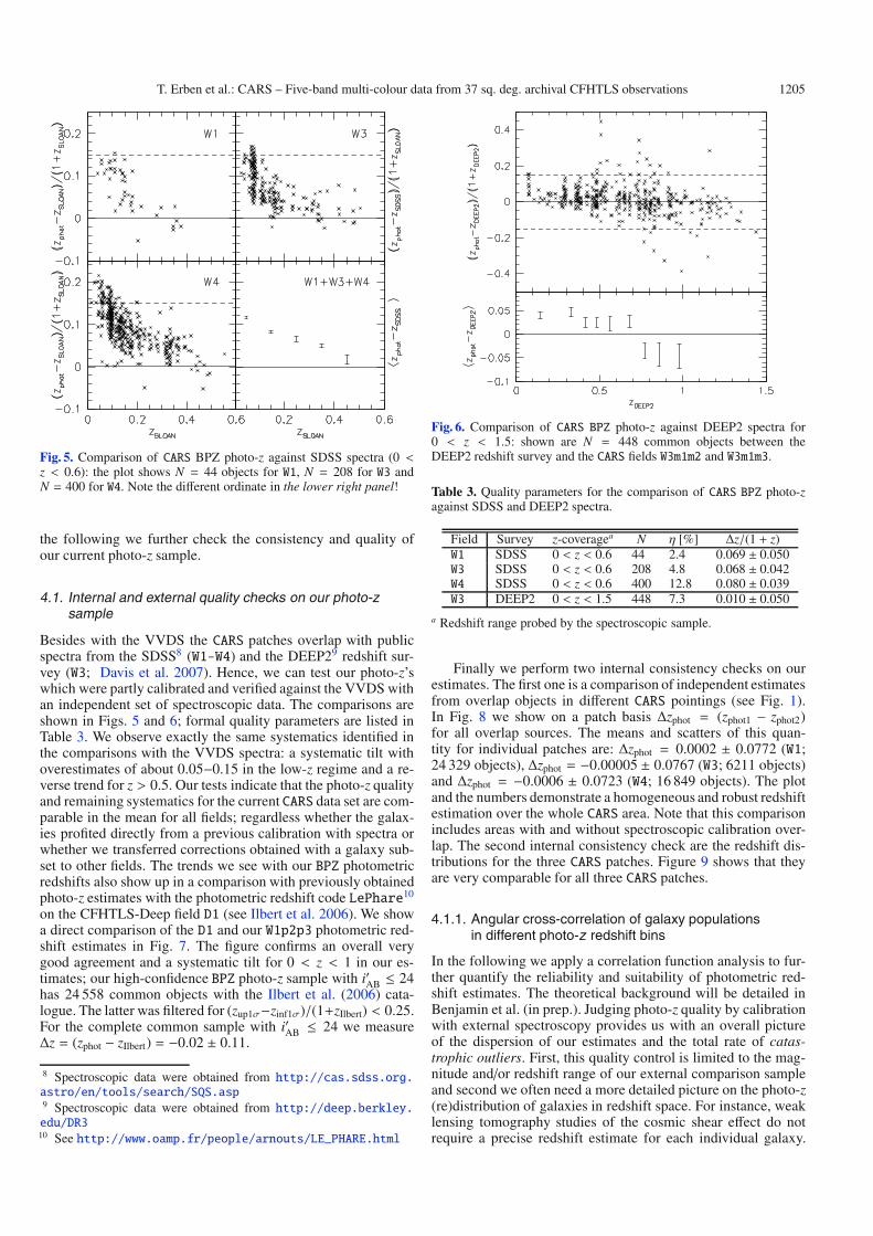
Fig. 5. Comparison of CARS BPZ photo-z against SDSS spectra (0 <z < 0.6): the plot shows N = 44 objects for W1, N = 208 for W3 andN = 400 for W4. Note the different ordinate in the lower right panel!

the following we further check the consistency and quality ofour current photo-z sample.

4.1. Internal and external quality checks on our photo-zsample

Besides with the VVDS the CARS patches overlap with publicspectra from the SDSS8 (W1-W4) and the DEEP29 redshift sur-vey (W3; Davis et al. 2007). Hence, we can test our photo-z’swhich were partly calibrated and verified against the VVDS withan independent set of spectroscopic data. The comparisons areshown in Figs. 5 and 6; formal quality parameters are listed inTable 3. We observe exactly the same systematics identified inthe comparisons with the VVDS spectra: a systematic tilt withoverestimates of about 0.05−0.15 in the low-z regime and a re-verse trend for z > 0.5. Our tests indicate that the photo-z qualityand remaining systematics for the current CARS data set are com-parable in the mean for all fields; regardless whether the galax-ies profited directly from a previous calibration with spectra orwhether we transferred corrections obtained with a galaxy sub-set to other fields. The trends we see with our BPZ photometricredshifts also show up in a comparison with previously obtainedphoto-z estimates with the photometric redshift code LePhare10

on the CFHTLS-Deep field D1 (see Ilbert et al. 2006). We showa direct comparison of the D1 and our W1p2p3 photometric red-shift estimates in Fig. 7. The figure confirms an overall verygood agreement and a systematic tilt for 0 < z < 1 in our es-timates; our high-confidence BPZ photo-z sample with i′AB ≤ 24has 24 558 common objects with the Ilbert et al. (2006) cata-logue. The latter was filtered for (zup1σ−zinf1σ)/(1+zIlbert) < 0.25.For the complete common sample with i′AB ≤ 24 we measureΔz = (zphot − zIlbert) = −0.02 ± 0.11.

8 Spectroscopic data were obtained from http://cas.sdss.org.astro/en/tools/search/SQS.asp9 Spectroscopic data were obtained from http://deep.berkley.edu/DR310 See http://www.oamp.fr/people/arnouts/LE_PHARE.html

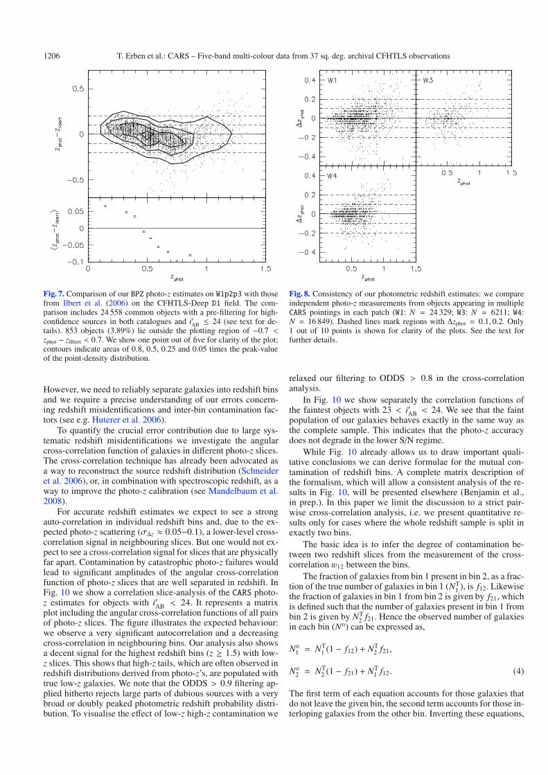
Fig. 6. Comparison of CARS BPZ photo-z against DEEP2 spectra for0 < z < 1.5: shown are N = 448 common objects between theDEEP2 redshift survey and the CARS fields W3m1m2 and W3m1m3.

Table 3. Quality parameters for the comparison of CARS BPZ photo-zagainst SDSS and DEEP2 spectra.

Field Survey z-coveragea N η [%] Δz/(1 + z)W1 SDSS 0 < z < 0.6 44 2.4 0.069 ± 0.050W3 SDSS 0 < z < 0.6 208 4.8 0.068 ± 0.042W4 SDSS 0 < z < 0.6 400 12.8 0.080 ± 0.039W3 DEEP2 0 < z < 1.5 448 7.3 0.010 ± 0.050

a Redshift range probed by the spectroscopic sample.

Finally we perform two internal consistency checks on ourestimates. The first one is a comparison of independent estimatesfrom overlap objects in different CARS pointings (see Fig. 1).In Fig. 8 we show on a patch basis Δzphot = (zphot1 − zphot2)for all overlap sources. The means and scatters of this quan-tity for individual patches are: Δzphot = 0.0002 ± 0.0772 (W1;24 329 objects), Δzphot = −0.00005 ± 0.0767 (W3; 6211 objects)and Δzphot = −0.0006 ± 0.0723 (W4; 16 849 objects). The plotand the numbers demonstrate a homogeneous and robust redshiftestimation over the whole CARS area. Note that this comparisonincludes areas with and without spectroscopic calibration over-lap. The second internal consistency check are the redshift dis-tributions for the three CARS patches. Figure 9 shows that theyare very comparable for all three CARS patches.

4.1.1. Angular cross-correlation of galaxy populationsin different photo-z redshift bins

In the following we apply a correlation function analysis to fur-ther quantify the reliability and suitability of photometric red-shift estimates. The theoretical background will be detailed inBenjamin et al. (in prep.). Judging photo-z quality by calibrationwith external spectroscopy provides us with an overall pictureof the dispersion of our estimates and the total rate of catas-trophic outliers. First, this quality control is limited to the mag-nitude and/or redshift range of our external comparison sampleand second we often need a more detailed picture on the photo-z(re)distribution of galaxies in redshift space. For instance, weaklensing tomography studies of the cosmic shear effect do notrequire a precise redshift estimate for each individual galaxy.

1206 T. Erben et al.: CARS – Five-band multi-colour data from 37 sq. deg. archival CFHTLS observations

Fig. 7. Comparison of our BPZ photo-z estimates on W1p2p3 with thosefrom Ilbert et al. (2006) on the CFHTLS-Deep D1 field. The com-parison includes 24 558 common objects with a pre-filtering for high-confidence sources in both catalogues and i′AB ≤ 24 (see text for de-tails). 853 objects (3.89%) lie outside the plotting region of −0.7 <zphot − zIlbert < 0.7. We show one point out of five for clarity of the plot;contours indicate areas of 0.8, 0.5, 0.25 and 0.05 times the peak-valueof the point-density distribution.

However, we need to reliably separate galaxies into redshift binsand we require a precise understanding of our errors concern-ing redshift misidentifications and inter-bin contamination fac-tors (see e.g. Huterer et al. 2006).

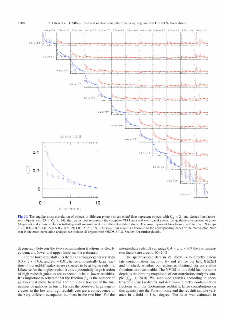
To quantify the crucial error contribution due to large sys-tematic redshift misidentifications we investigate the angularcross-correlation function of galaxies in different photo-z slices.The cross-correlation technique has already been advocated asa way to reconstruct the source redshift distribution (Schneideret al. 2006), or, in combination with spectroscopic redshift, as away to improve the photo-z calibration (see Mandelbaum et al.2008).

For accurate redshift estimates we expect to see a strongauto-correlation in individual redshift bins and, due to the ex-pected photo-z scattering (σΔz ≈ 0.05−0.1), a lower-level cross-correlation signal in neighbouring slices. But one would not ex-pect to see a cross-correlation signal for slices that are physicallyfar apart. Contamination by catastrophic photo-z failures wouldlead to significant amplitudes of the angular cross-correlationfunction of photo-z slices that are well separated in redshift. InFig. 10 we show a correlation slice-analysis of the CARS photo-z estimates for objects with i′AB < 24. It represents a matrixplot including the angular cross-correlation functions of all pairsof photo-z slices. The figure illustrates the expected behaviour:we observe a very significant autocorrelation and a decreasingcross-correlation in neighbouring bins. Our analysis also showsa decent signal for the highest redshift bins (z ≥ 1.5) with low-z slices. This shows that high-z tails, which are often observed inredshift distributions derived from photo-z’s, are populated withtrue low-z galaxies. We note that the ODDS > 0.9 filtering ap-plied hitherto rejects large parts of dubious sources with a verybroad or doubly peaked photometric redshift probability distri-bution. To visualise the effect of low-z high-z contamination we

Fig. 8. Consistency of our photometric redshift estimates: we compareindependent photo-z measurements from objects appearing in multipleCARS pointings in each patch (W1: N = 24 329; W3: N = 6211; W4:N = 16 849). Dashed lines mark regions with Δzphot = 0.1, 0.2. Only1 out of 10 points is shown for clarity of the plots. See the text forfurther details.

relaxed our filtering to ODDS > 0.8 in the cross-correlationanalysis.

In Fig. 10 we show separately the correlation functions ofthe faintest objects with 23 < i′AB < 24. We see that the faintpopulation of our galaxies behaves exactly in the same way asthe complete sample. This indicates that the photo-z accuracydoes not degrade in the lower S/N regime.

While Fig. 10 already allows us to draw important quali-tative conclusions we can derive formulae for the mutual con-tamination of redshift bins. A complete matrix description ofthe formalism, which will allow a consistent analysis of the re-sults in Fig. 10, will be presented elsewhere (Benjamin et al.,in prep.). In this paper we limit the discussion to a strict pair-wise cross-correlation analysis, i.e. we present quantitative re-sults only for cases where the whole redshift sample is split inexactly two bins.

The basic idea is to infer the degree of contamination be-tween two redshift slices from the measurement of the cross-correlation w12 between the bins.

The fraction of galaxies from bin 1 present in bin 2, as a frac-tion of the true number of galaxies in bin 1 (NT

1 ), is f12. Likewisethe fraction of galaxies in bin 1 from bin 2 is given by f21, whichis defined such that the number of galaxies present in bin 1 frombin 2 is given by NT

2 f21. Hence the observed number of galaxiesin each bin (No) can be expressed as,

No1 = NT

1 (1 − f12) + NT2 f21,

No2 = NT

2 (1 − f21) + NT1 f12. (4)

The first term of each equation accounts for those galaxies thatdo not leave the given bin, the second term accounts for those in-terloping galaxies from the other bin. Inverting these equations,

T. Erben et al.: CARS – Five-band multi-colour data from 37 sq. deg. archival CFHTLS observations 1207

Fig. 9. Normalised distributions of our high-confidence photometricredshift estimates for all CARS patches (W1: N = 205 956 for 17 <i′AB < 22 and N = 487 593 for 22 < i′AB < 24; W3: N = 52 295 for17 < i′AB < 22 and N = 119 589 for 22 < i′AB < 24; W4: N = 104 417for 17 < i′AB < 22 and N = 252 969 for 22 < i′AB < 24); all distributionshave only very few objects beyond redshift 2 (not shown).

the true number of galaxies can be expressed as a function of theobserved numbers and the fractions f12 and f21,

NT1 =

No1 − f21(No

1 + No2 )

1 − f12 − f21,

NT2 =

No2 − f12(No

1 + No2 )

1 − f12 − f21· (5)

Note that No1+No

2 = NT1 +NT

2 , thus the total number of galaxies ispreserved, as should be the case. It is also obvious that for caseswhere f12 + f21 is unity there is a zero in the denominator. Whatis less clear, is that in these cases the numerator is also zero,which can be seen by plugging Eq. (4) into the numerator. In thiscase the system of equations is degenerate, and will not admit aunique solution. This should not pose a practical limitation sinceit is expected that the fractional contamination between bins issmall, and specifically less than 0.5.

In order to calculate how the cross-correlation function ischanged for non-vanishing coefficients f12, f21, it is sufficient toconsider the natural estimator of the angular correlation func-tion, as opposed to that presented by Landy & Szalay (1993).The natural estimator works well at small and intermediatescales where edge effects are not an issue, provided that thereis a sufficient density of points (see Kerscher et al. 2000, for acomparison of the estimators). The observed angular cross cor-relation functions are given by,

1 + ωo11 =

(D1D1)oθ

(R1R2)θ, (6)

1 + ωo12 =

(D1D2)oθ

(R1R2)θ, (7)

where (D1D1)oθ is the observed number of pairs separated by an-

gle θ within bin 1, similarly (D1D2)oθ is the number of pairs be-

tween bins 1 and 2, and (R1R2)θ is the number of pairs betweenobjects from random fields of identical geometry.

Considering how galaxy pairs are split between the twobins 1 and 2, one can show that the observed number of pairsdepends on a combination of the true number of pairs and thecontamination fractions:

(D1D2)oθ = (D1D2)T

θ ((1 − f12)(1 − f21) + f21 f12)

+(D1D1)Tθ (1 − f12) f12 + (D2D2)T

θ f21(1 − f21). (8)

Plugging this relation into Eq. (7), and noting that theterm (D1D2)o

θ/(R1R2)θ must be normalised by NR1 NR

2 /No1 No

2 ,where NR

1,2 is the number of objects in the random samples,the following equation can be derived for the observed angularcross-correlation function,

1 + ωo12 = (1 + ωT

11)(NT

1 )2

No1 No

2

f12(1 − f12)

+(1 + ωT22)

(NT2 )2

No1 No

2

f21(1 − f21)

+(1 + ωT12)

NT1 NT

2

No1 No

2

(1 − f12 − f21 + 2 f12 f21). (9)

Note that the observed cross-correlation function depends onthe unknown true number of galaxies in the bins and the un-known true auto-correlation function. The true galaxy numbercan be expressed in terms of the observed number of galax-ies and the contamination fractions via Eq. (5). It is possibleto express the true auto-correlation as functions of contamina-tion fractions, the number of observed galaxies and the observedauto-correlation functions (Benjamin et al., in prep.),

ωT11 = ω

o11

⎛⎜⎜⎜⎜⎝No

1

NT1

⎞⎟⎟⎟⎟⎠2

(1 − f21)2

(1 − f12)2(1 − f21)2 − f 212 f 2

21

−ωo22

⎛⎜⎜⎜⎜⎝No

2

NT1

⎞⎟⎟⎟⎟⎠2 f 2

21

(1 − f12)2(1 − f21)2 − f 212 f 2

21

−ωT12

⎛⎜⎜⎜⎜⎝NT

2

NT1

⎞⎟⎟⎟⎟⎠ 2 f21(1 − f21)(1 − f12)(1 − f21) + f12 f21

· (10)

By exchanging 1 and 2 in Eq. (10) an equivalent expression forthe auto-correlation of bin 2 is obtained. To finally use Eqs. (9)and (10) we make the explicit assumption that the true cross-correlation between the two redshift bins is zero (ωT

12 = 0), i.e.all the observed cross-correlation is due to contamination. Thisprescription allows us to use the observed correlation functionsand number of galaxies to determine the contamination frac-tions, f12 and f21, for a pair of redshift bins.

We note that the outlined formalism cannot be trivially ex-tended to a multi-bin setup, since it assumes a pair of bins andignores possible contamination from other redshifts. However,it already allows us to recover the fraction of objects that crossa given redshift zcut due to photometric redshift errors, and ananalysis can be done as a function of zcut.

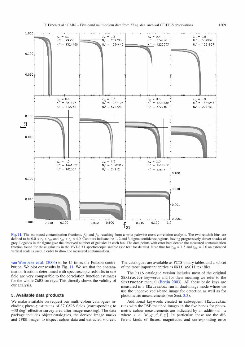
We apply the pairwise analysis on our data by cutting itat zcut = 0.2; 0.3; 0.4; 0.5; 0.6; 0.7; 0.8; 0.9; 1.0; 1.5; 2.0 yieldinga low redshift bin 0.0 < z1 < zcut and a high redshift binzcut < z2 < 4.0. The angular auto and cross-correlation functionsfrom the pair of bins are used to estimate the contamination frac-tions f12 and f21 by fitting the observed cross-correlation withEq. (9). The analysis was performed with eleven equally spacedcross-correlation bins ranging from 0.′9 to 10.′0. We checkedwith an analysis of three and five bins that our results do not de-pend significantly on this choice. This step is followed by a min-imum chi-square analysis and the likelihood contours in the con-tamination fraction parameter space are presented in Fig. 11. The

1208 T. Erben et al.: CARS – Five-band multi-colour data from 37 sq. deg. archival CFHTLS observations

0.1 1 10

0

0.2

0.4

Fig. 10. The angular cross-correlation of objects in different photo-z slices (solid lines represent objects with i′AB < 24 and dashed lines repre-sent objects with 23 < i′AB < 24): the matrix plot represents the complete CARS area and each panel shows the qualitative behaviour of auto-(diagonal) and crosscorrelation (off-diagonal) measurement for different redshift slices. The rows represent bins from z = 0 to z = 3.9 (stepsz = 0.0; 0.2; 0.3; 0.4; 0.5; 0.6; 0.7; 0.8; 0.9; 1.0; 1.5; 2.0; 3.9). The lower left panel is a zoom-in to the corresponding panel of the matrix plot. Notethat in the cross-correlation analysis we include all objects with ODDS > 0.8. See text for further details.

degeneracy between the two contamination fractions is clearlyevident, and lower and upper limits can be estimated.

For the lowest redshift cuts there is a strong degeneracy, with0.0 < f12 < 0.6, and f21 ∼ 0.01, hence a potentially large frac-tion of low redshift galaxies are expected to be at higher redshift.Likewise for the highest redshift cuts a potentially large fractionof high redshift galaxies are expected to be at lower redshifts.It is important to reiterate that the fraction f12 is the number ofgalaxies that move from bin 1 to bin 2 as a fraction of the truenumber of galaxies in bin 1. Hence, the observed large degen-eracies in the low and high redshift cuts are a consequence ofthe very different occupation numbers in the two bins. For the

intermediate redshift cut range 0.4 < zcut < 0.9 the contamina-tion factors are around 10−20%.

The spectroscopic data in W1 allow us to directly calcu-late contamination fractions f12 and f21 for the field W1p2p3and to check whether our estimates obtained via correlationfunctions are reasonable. The VVDS in this field has the samedepth as the limiting magnitude of our correlation analysis sam-ple (i′AB ≤ 24.0). We subdivide galaxies according to spec-troscopic (true) redshifts and determine directly contaminationfractions with the photometric redshifts. Error contributions onthis quantity are the Poisson noise and the redshift sample vari-ance in a field of 1 sq. degree. The latter was estimated in

T. Erben et al.: CARS – Five-band multi-colour data from 37 sq. deg. archival CFHTLS observations 1209

Fig. 11. The estimated contamination fractions, f12 and f21 resulting from a strict pairwise cross-correlation analysis. The two redshift bins aredefined to be 0.0 < z1 < zcut and zcut < z2 < 4.0. Contours indicate the 1, 2 and 3-sigma confidence regions, having progressively darker shades ofgrey. Legends in the figure give the observed number of galaxies in each bin. The data points with error bars denote the measured contaminationfraction found for those galaxies in the VVDS W1 spectroscopic sample (see text for details). Note that for zcut = 1.5 and zcut = 2.0 an extendedvertical scale is used in order to show the measured contamination.

van Waerbeke et al. (2006) to be 15 times the Poisson contri-bution. We plot our results in Fig. 11. We see that the contam-ination fractions determined with spectroscopic redshifts in onefield are very comparable to the correlation function estimatesfor the whole CARS surveys. This directly shows the validity ofour analysis.

5. Available data productsWe make available on request our multi-colour catalogues in-cluding photo-z estimates of 37 CARS fields (corresponding to∼30 deg2 effective survey area after image masking). The datapackage includes object catalogues, the derived image masksand JPEG images to inspect colour data and extracted sources.

The catalogues are available as FITS binary tables and a subsetof the most important entries as UNIX-ASCII text files.

The FITS catalogue version includes most of the originalSExtractor keywords and for their meaning we refer to theSExtractor manual (Bertin 2003). All these basic keys aremeasured in a SExtractor run in dual-image mode where weuse the unconvolved i-band image for detection as well as forphotometric measurements (see Sect. 3.3).

Additional keywords created in subsequent SExtractorruns with the PSF-matched images in the five bands for photo-metric colour measurements are indicated by an additional _xwhere x ∈ [u∗, g′, r′, i′, z′]. In particular, these are the dif-ferent kinds of fluxes, magnitudes and corresponding error

1210 T. Erben et al.: CARS – Five-band multi-colour data from 37 sq. deg. archival CFHTLS observations

Table 4. Description of the most important FITS keys in the CARS multi-colour catalogues.

key name Description Unit Measured on ASCII catalogueSeqNr Running object number − − √ALPHA_J2000 Right ascension degree unconvolved i′-band image

√DELTA_J2000 Declination degree unconvolved i′-band image

√Xpos x pixel position pixel unconvolved i′-band image

√Ypos y pixel position pixel unconvolved i′-band image

√MAG_AUTO total i′-band magnitude mag unconvolved i′-band image

√MAGERR_AUTO total i′-band magnitude error mag unconvolved i′-band image

√MAG_ISO_xa isophotal magnitude in x-band mag PSF-equalised x-band image

√MAGERR_ISO_x isophotal magnitude error in x-band mag PSF-equalised x-band image

√MAG_APER_xb aperture magnitude vector in x-band mag PSF-equalised x-band image

√MAGERR_APER_x aperture magnitude error vector in x-band mag PSF-equalised x-band image

√FWHM_WORLD FWHM assuming a Gaussian core degree unconvolved i′-band image

√FLUX_RADIUS half-light-radius pixel unconvolved i′-band image

√A_WORLD profile rms along major axis degree unconvolved i′-band image

√B_WORLD profile rms along minor axis degree unconvolved i′-band image

√THETA_J2000 position angle degree unconvolved i′-band image

√CLASS_STAR star-galaxy classifier − unconvolved i′-band image

√Flag SExtractor extraction flags − unconvolved i′-band image

√FLUX_ISO_x isophotal flux in x-band ADU/s PSF-equalised x-band image −FLUXERR_ISO_x isophotal flux error in x-band ADU/s PSF-equalised x-band image −FLUX_APER_x aperture flux vector in x-band ADU/s PSF-equalised x-band image −FLUXERR_APER_x aperture flux error vector in x-band ADU/s PSF-equalised x-band image −MAG_LIM_x limiting magnitude in x-band mag unconvolved x-band image

√Z_B Bayesian photo-z estimate − − √Z_B_MIN lower bound of the 95% confidence interval − − −Z_B_MAX upper bound of the 95% confidence interval − − −T_B best-fit spectral typec − − √ODDS empirical oddsd − − √NBPZ_GOODFILT filters with reliable photometry − − √NBPZ_BADFILT filters with MAGERR_ISO ≥ 1.0 − √NBPZ_LIMFILT filters with MAG_ISO_x ≥ MAG_LIM_x − − √MASK global mask keye − − √

a x ∈ [u, g, r, i, z]; b The ASCII catalogue version contains one aperture magnitude at a diameter of 1.′′86. The FITS version lists 24 aperturemagnitudes for diameters from 0.′′744 to 10.′′23; c Ell = 1, Sbc = 2, Scd = 3, Im = 4, SB3 = 5, SB2 = 6, plus two interpolated types in colour-redshiftspace between each pair of these basis templates. Intermediate best-fit templates are indicated by a floating point number for T_B; d integratedprobability inside an interval which is such that it contains 95% probability for a single Gaussian; e unification of the different masks described inSect. 3.4.

estimates (e.g. FLUX_AUTO_x, FLUXERR_AUTO_x, MAG_ISO_x,MAGERR_ISO_x, etc.); note that magnitude error estimates in thecatalogues do not take into account systematic zeropoint off-sets but only statistical errors due to photon noise. We estimate24 different aperture fluxes and magnitudes with diameters rang-ing from 4 to 55 pixels (=̂0.′′744 to 10.′′23). We add the 1σ limit-ing magnitudes MAG_LIM_x as described in Sect. 3.2. All magni-tudes are provided in MegaPrime instrumental AB magnitudes.We note that we did not apply any magnitude correction tothe catalogue entries also if our tests performed in Sect. A.4might justify them. This especially applies for discrepanciespresent in the u∗-band calibration of the W3 and W4 pointings (seeSect. A.4). To allow an easy identification of objects with prob-lematic photometry we add the flags NBPZ_GOODFILT indicatingthe number of filters with reliable photometry, NBPZ_BADFILTgiving the number of filters with MAGERR_ISO_x ≥ 1.0 andNBPZ_LIMFILT listing the number of filters with MAG_ISO_xfainter than our formal magnitude limit (see Sect. 2). Which ofthese three properties applies to which filters is encoded in addi-tional keys.

Furthermore, we provide a global mask key MASK which is 0for objects that do not lie inside one of our object masks and1 otherwise. This key takes into account all masks from our ob-ject density, bright star and asteroid track analyses as describedin Sect. 3.4.

Finally, the catalogues contain photo-z relevant quantitiesfrom the output of BPZ. Besides the Bayesian redshift estimate,Z_B, we include the ODDS probability, the SED correspond-ing to the Bayesian redshift (T_B), the corresponding χ2, the95% confidence interval (Z_B_MIN and Z_B_MAX) as well asthe maximum-likelihood redshift and type estimate (Z_ML andT_ML), which are put out by BPZ before the prior is applied.

The most important catalogue entries are summarised inTable 4.

6. Summary and conclusions

We have presented high-quality five-band multi-colour data from37 sq. deg. of the CARS survey. We gave a detailed descriptionof our data-handling procedures ranging from data selection tothe final catalogues including a first set of photometric redshiftestimates. Our algorithms provide an accurate astrometric align-ment on the sub-pixel level to extract precise object colour in-formation. For the large majority of our data the Elixir pho-tometric information allows us to derive an unbiased absolutephotometric calibration with a scatter of σ ≈ 0.02−0.05 magon a pointing basis for g′r′i′z′; tests against the officialTERAPIX T0003 CFHTLS-data release show very significantzeropoint offsets for four out of 93 common fields. In u∗ direct

T. Erben et al.: CARS – Five-band multi-colour data from 37 sq. deg. archival CFHTLS observations 1211

comparisons with SDSS suggest that our zeropoints are system-atically about 0.1 mag too faint.

We showed that our colour catalogues allow, with the helpof spectroscopic information, the estimation of reliable photo-metric redshift estimates with the method of Benitez (2000).In our 37 sq. deg. survey (about 30 sq. deg. in unmaskedareas) we detect about 3.9 million objects classified as galax-ies (SExtractor CLASS_STAR < 0.95). From those about1.45 million (10−15 galaxies per sq. arcmin) have a formally re-liable photo-z estimate with ODDS > 0.9 (completeness 37.2%).Comparing our photo-z estimates with external spectroscopicdata we find an overall performance of σ(Δz/(1 + z)) ≈0.04−0.05 up to i′AB ≈ 24 with an outlier rate of η ≈ 1−3%. Weapplied a cross-correlation analysis to qualitatively investigateredshift slice contamination between samples in different red-shift bins. It indicates significant contamination of neighbouringredshift slices with a width of Δz ≈ 0.1 and a dying correla-tion signal for bins more than Δz ≈ 0.3 apart. Catastrophic out-liers occur between low-z bins and galaxies with an estimate ofzphot ≥ 1.5. We performed a more quantitative analysis only forthe case when our whole redshift sample is divided in exactlytwo redshift bins. With the help of spectroscopic redshifts fromthe deep part of the VVDS it reconfirms the homogeneity of ourphoto-z sample over the entire CARS area. A more complete, in-depth analysis with the correlation function technique will bepresented in Benjamin et al. (in prep.).

We note that the catalogues and the estimation of photo-z’swas optimised for studies in the regime 0 < z < 1.4 and ob-jects with a larger estimate should be filtered. The current cat-alogues are not suited for studies of the high-z regime such asu∗-band drop-out searches. While the photo-z performance ac-cording to formal parameters is very good our estimates show asystematic tilt for 0 < z < 1 (higher redshift ranges cannot beverified due to the lack of spectroscopic information). Our esti-mates are too high by Δz ≈ 0.1 for low z and the bias decreaseslinearly to reach about Δz ≈ −0.1 for z ≈ 1. The zero-crossingof the tilt is at z ≈ 0.5. The mean bias is about 〈Δz〉 ≈ 0.03 forz < 0.5 and about 〈Δz〉 ≈ −0.03 for 0.5 < z < 1. Improved andbias-free BPZ photo-z estimates will be presented in Hildebrandtet al. (in preparation). Additionally, photo-z estimates with themethod of Bender et al. (2001) are analysed and compared toour current work in Brimioulle et al. (2008). An independent ef-fort to derive photo-z estimates on the same survey area with theTERAPIX T0004 release is undertaken in Coupon et al. (2008).

The presented catalogues mark the first step for the primaryscience goal of CARS in the CFHTLS-Wide area: the assemblingof a galaxy cluster sample from low to high redshift and itssubsequent exploitation for cosmological studies. For the sec-ond step in this effort, our multi-colour data are currently be-ing used on several cluster detection algorithms: the Voronoitessellation technique from Ramella et al. (2001), the Postmanmatched filter algorithm (see Postman et al. 1996) and the Red-Cluster Sequence technique (see Gladders & Yee 2000).

To trigger a larger variety of follow-up studies we makeavailable our catalogues on request.

Acknowledgements. We thank Brice Ménard for help with the redshift cross-correlation analysis and Stephen Gwyn for clarifications on his MegaPipe pro-cessing pipeline. We thank the staff at the Canada-France-Hawaii Telescope andat the TERAPIX data centre in Paris for delivering high-quality CFHTLS Surveyproducts and excellent image processing software to the astronomical commu-nity. The anonymous referee helped us to improve the manuscript significantly.We acknowledge use of the Canadian Astronomy Data Centre, which is operatedby the Dominion Astrophysical Observatory for the National Research Councilof Canada’s Herzberg Institute of Astrophysics. This work was supportedby the DFG Sonderforschungsbereich 375 “Astro-Teilchenphysik”, the DFG

priority program SPP-1177 “Witnesses of Cosmic History: Formation and evo-lution of black holes, galaxies and their environment” (project IDs ER327/2-2,SCHN 342/7–1, Se1038/1), the German Ministry for Science and Education(BMBF) through DESY under the project 05AV5PDA/3 and the TR33 “TheDark Universe”. H. H. and M. L. are supported by the European DUEL RTN,project MRTN-CT-2006-036133. T.S. acknowledges financial support from theNetherlands Organization for Scientific Research (NWO). K.H. is supported bythe Research council of Norway, project number 177254/V30. L.v.W. and J.B.acknowledge support by NSERC and CIfAR. Part of the data reduction de-scribed in this work was performed on CFI funded equipment under projectgrant #10052. M.L. thanks the University of Bonn and the University of BritishColumbia for hospitality.

Appendix A: Details on the data handling of CARSobservations

In this Appendix we give a more detailed description on our datahandling procedures of the CARS survey. The excellent Elixirpreprocessing of the CARS data and the available meta-data in-formation (see below) allowed us to build up a complete sur-vey pipeline starting from data retrieval up to final co-added sci-ence images. The construction of our data-processing pipelineand many choices for our data-handling as described below weredriven by the following two requirements:

1. The system allows a 100% automatic processing of the datawith the need for manual intervention only at the final veri-fication stage of co-added science images. This particularlyforbids manual passes through all individual Elixir imageseither to visually grade data or to remove/mask artefacts.We needed to automatically reject problematic exposures orparts of them from the whole analysis or we need to deal withremaining defects at the level of the final science images.For instance, our automatic satellite track removal modulereliably detects and removes about 95% of all bright satel-lite trails. If necessary, the remaining 5% need to be maskedmanually in the final science images.

2. We want to independently and incrementally process indi-vidual pointings as soon as the full five band coverage of aparticular area is becoming publicly available.

We completely achieved the first goal and the complete data pro-cessing of the CARS data is done by one of the authors with twocomputers (a double processor Athlon2800+ with 4 GB Virtualmemory and a quad processor/dual core AMD Opteron 885 with11 GB of RAM) and a total disk storage capacity of about10 Terabytes. The second goal could not be met for the pho-tometric calibration of several fields and we needed to use in-formation from adjacent pointings to obtain an absolute fluxcalibration (see below).

Most of our algorithms to process optical data from multi-chip cameras were described in Erben et al. (2005) andHildebrandt et al. (2006) in the context of GaBoDS data(see e. g. Schirmer et al. 2003) from the 8-chip instrumentWFI@MPG/ESO2.2m. We therefore limit the discussion to pe-culiarities of the CARS data, necessary pipeline upgrades due tothe four times larger field-of-view of MegaPrime and quality as-sessments of our final science images.

A.1. Data preselection and retrieval

As described in Sect. 2, the starting point of the currentCARS data set are the Elixir preprocessed images fromthe CFHTLS-Wide Survey. Besides the images, compre-hensive information on the current status of the Surveyand the observed data is available in the form of a CFHTLS

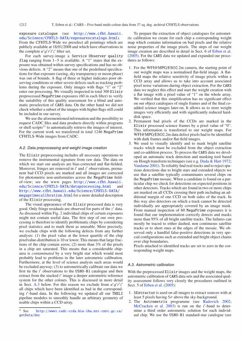
1212 T. Erben et al.: CARS – Five-band multi-colour data from 37 sq. deg. archival CFHTLS observations

exposure catalogue (see http://www.cfht.hawaii.edu/Science/CFHTLS-DATA/exposurescatalogs.html).From the CFHTLS-Wide we preselect all pointings which arepublicly available at 18/01/2008 and which have observations inthe complete u∗g′r′i′z′ filter set.

For each survey-image a Service Observer qualityflag ranging from 1−5 is available. A “1” states that the ex-posure was obtained within survey specifications and has no ob-vious defects. A “2” means that one of the predefined specifica-tions for that exposure (seeing, sky transparency or moon phase)was out of bounds. A flag of three or higher indicates poor ob-serving conditions or other severe defects such as tracking prob-lems during the exposure. Only images with flags “1” or “2”enter our processing. We visually inspected in total 300 Elixirpreprocessed MegaPrime exposures (60 in each filter) to verifythe suitability of this quality assessment for a blind and auto-matic preselection of CARS data. On the other hand we did notcheck whether a subset of the images with higher flags still couldbe included in our survey.

We use the aforementioned information and the possibility torequest CADC files and data products directly within programsor shell scripts11 to automatically retrieve the images of interest.For the current work we transferred in total 1246 MegaPrimeCFHTLS-Wide images from CADC.

A.2. Data preprocessing and weight image creation

The Elixir preprocessing includes all necessary operations toremove the instrumental signature from raw data. The data onwhich we start our analysis are bias-corrected and flat-fielded.Moreover, fringes are removed in i′ and z′ observations, perma-nent bad CCD pixels are marked and all images are correctedfor photometric non-uniformities across the MegaPrime field-of-view; see the www pages http://www.cfht.hawaii.edu/Science/CFHTLS-DATA/dataprocessing.html andhttp://www.cfht.hawaii.edu/Science/CFHTLS-DATA/megaprimecalibration.html for a more detailed descriptionof the Elixir processing.

The visual appearance of the Elixir processed data is verygood. Only fringe residuals are observed for parts of the z′ data.As discussed within Fig. 2 individual chips of certain exposuresmight not contain useful data. The first step of our own pro-cessing is therefore to identify problematic chips by consideringpixel statistics and to mark them as unusable. More precisely,we exclude chips with the following defects from any furtheranalysis: (1) the pixel value at the lower quartile of the chippixelvalue-distribution is 10 or lower. This means that large frac-tions of the chip contain zeros; (2) more than 3% of the pixelsin a chip are saturated. This means that a considerable chip-area is contaminated by a very bright star which would mostprobably lead to problems in the later astrometric calibration.Furthermore, at the level of science analysis such areas wouldbe excluded anyway; (3) to astrometrically calibrate our data wefirst tie the i′ observations to the USNO-B1 catalogue and thenextract from the stacked i′ image a deeper astrometric referencesystem for the other colours. This is discussed in more detailin Sect. A.3 below. For this reason we exclude from u∗g′r′z′all chips which have been identified as bad in the correspond-ing i′-band data. In the following we updated all our THELIpipeline modules to smoothly handle an arbitrary geometry ofusable chips within a CCD-array.

11 See http://www1.cadc-ccda.hia-iha.nrc-cnrc.gc.ca/getData/doc

To prepare the extraction of object catalogues for astromet-ric calibration we create for each chip a corresponding weightmap which contains information on bad pixels and the relativenoise properties of the image pixels. The steps of our weightimage creation are described in detail in Sect. 6 of Erben et al.(2005). For the CARS data we updated and expanded our proce-dures as follows:

1. For the WFI@MPG/ESO2.2m camera, the starting point ofour weight maps was a normalised flat-field image. A flat-field maps the relative sensitivity of image pixels within aCCD array and allows us to take into account associatedpixel noise variations during object extraction. For the CARSdata we neglect this effect and start the weight creation witha flat image with a pixel value of “1” on the whole array.We verified that this simplification has no significant effecton our object catalogues of single frames and of the final co-added science images later-on. It allows us to store weightimages very efficiently and with significantly reduced hard-disk space.

2. Permanent bad pixels of the CCDs are marked in theElixir processed science frames by a pixel value of “0”.This information is transferred to our weight maps. ForWFI@MPG/ESO2.2m data defect pixels had to be identifiedwith dark frames and/or flat-field images.

3. We used to visually identify and to mask bright satellitetracks which must be excluded from the object extractionand co-addition process. To process the CARS data we devel-oped an automatic track detection and masking tool basedon Hough transform techniques (see e.g. Duda & Hart 1972;Vandame 2001). To reliably find real tracks and to reject spu-rious detections due to bright stars and extended objects weuse that a satellite typically contaminates several chips onthe MegaPrimemosaic. When a candidate is found on a par-ticular chip we check for detections on expected positions inother detectors. Tracks which are found in two or more chipsare masked on all CCDs crossing their path including an ad-ditional margin of one CCD on both sides of the track. Inthis way also detectors on which a track cannot be detectedindividually are appropriately covered by an image mask.From manual inspection of 60 MegaPrime exposures it isfound that our implementation correctly detects and masksmore than 95% of all bright satellite tracks. The failures canmostly be traced to either dashed, non continuous satellitetracks or to short ones at the edges of the mosaic. We ob-served only a handful false-positive detections in very spe-cial configurations such as extended and bright object chainsover chip boundaries.Pixels attached to identified tracks are set to zero in the cor-responding weight maps.

A.3. Astrometric calibration

With the preprocessed Elixir images and the weight maps, theastrometric calibration of CARS data sets and the associated qual-ity assessment follows very closely the procedures outlined inSect. 5 of Erben et al. (2005):

1. SExtractor is used on all images to extract sources with atleast 5 pixels having 5σ above the sky-background.

2. The Astrometrix programme (see Radovich 2002;McCracken et al. 2003) is run on the i′-band to deter-mine a third order astrometric solution for each individ-ual chip. We use the USNO-B1 standard-star catalogue (see

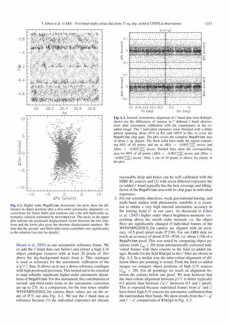
T. Erben et al.: CARS – Five-band multi-colour data from 37 sq. deg. archival CFHTLS observations 1213

Fig. A.1. Higher order MegaPrime distortions: the plots show the dif-ference in object position after a first-order astrometric alignment, i.e.corrections for linear shifts and rotations and a the full third-order as-trometric solution estimated by Astrometrix. The sticks in the upperplot indicate the positional displacement vector between the two solu-tions and the lower plot gives the absolute displacement numbers. Wenote that the second- and third-order terms contribute very significantlyto the solution (see text for details).

Monet et al. 2003) as our astrometric reference frame. Weco-add the i′-band data (see below) and extract a high S/Nobject catalogue (sources with at least 20 pixels of 20σabove the sky-background noise) from it. This catalogueis used as reference for the astrometric calibration of theu∗g′r′z′ data. It allows us to use a dense reference cataloguewith high positional precision. This turned out to be essentialto map robustly significant higher-order astrometric distor-tions of MegaPrime. For this instrument, the contributions ofsecond- and third-order terms to the astrometric correctionare up to 2.′′0. As a comparison, for the four times smallerWFI@MPG/ESO2.2m camera these values are on the or-der of 0.′′5; see also Fig. A.1. We use the i′-band data asreference because (1) the individual exposures are already

Fig. A.2. Internal Astrometric alignment of i′-band data from W1m1p2:shown are the differences of sources in 7 dithered i′-band observa-tions after astrometric calibration with the counterparts in the co-added image. The 7 individual exposures were obtained with a ditherpattern spanning about 45.′′0 in RA and 180.′′0 in Dec to cover theMegaPrime chip gaps. The plot covers the complete MegaPrime areaof about 1 sq. degree. The thick solid lines mark the region contain-ing 68% of all points and are at ΔRA = −0.003+0.029

−0.035 arcsec andΔDec = −0.002+0.031

−0.035 arcsec. Dashed lines show the correspondingarea for 90% of all points (ΔRA = −0.003+0.092

−0.099 arcsec and ΔDec =−0.002+0.081

−0.086) arcsec. Only 1 out of 10 points is shown for clarity ofthe plot.

reasonably deep and hence can be well calibrated with theUSNO-B1 sources and (2) with seven dithered exposures theco-added i′-band typically has the best coverage and filling-factor of the MegaPrime area with its chip gaps in individualexposures.

3. For our scientific objectives, weak gravitational lensing, andmulti-band studies with photometric redshifts it is essen-tial to obtain a very high internal astrometric accuracy inthe lensing band (i′ in our case). As discussed in Erbenet al. (2005) higher order object brightness-moments (ev-erything above the zeroth order moment, i.e. the objectflux) are significantly changed if individual frames of theWFI@MPG/ESO2.2m camera are aligned with an accu-racy >0.5 pixel (pixel scale 0.′′238). For our CARS data wereach an accuracy of about 0.′′03−0.′′04, i.e. about 1/5th of aMegaPrime pixel. This was tested by comparing object po-sitions (with i′AB < 20) from astrometrically corrected indi-vidual frames with their cousins in the final co-added im-ages. Results for the field W1m1p2 in the i′ filter are shown inFig. A.2. In a similar way the inter-colour alignment of dif-ferent filters per pointing is tested. From the final co-addedimages we compare object positions of high S/N sources(i′AB < 20). For all pointings we reach an alignment be-tween the colours below one pixel. We note however thatthe inter-colour alignment between g′r′i′ is better (typically0.5 pixels) than between i′u∗z′ (between 0.5 and 1 pixel).This is expected because individual frames from u∗ and z′have fewer high S/N sources for astrometric calibration thanthe intermediate filter bands. We show results from the i′ −g′and i′ − u∗ comparisons of W1m1p2 in Fig. A.3.

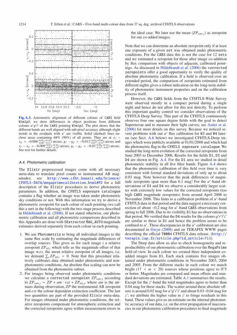
1214 T. Erben et al.: CARS – Five-band multi-colour data from 37 sq. deg. archival CFHTLS observations

Fig. A.3. Astrometric alignment of different colours of CARS fieldW1m1p2: we show differences in object positions from differentcolours u∗g′i′ of the CARS pointing W1m1p2. The plot shows that thedifferent bands are well aligned with sub-pixel accuracy although slighttrends in the residuals with u∗ are visible. Solid (dashed) lines en-close areas containing 68% (90%) of all points. They are at xi′ −xg′ = −0.006+0.05

−0.06(+0.10−0.11) arcsec, yi′ − yg′ = −0.012+0.04

−0.07(+0.09−0.12) arcsec and

xi′ − xu∗ = −0.009+0.07−0.09(+0.16

−0.18) arcsec, yi′ − yu∗ = −0.03+0.06−0.12(+0.14

−0.20) arcsec.See text for further details.

A.4. Photometric calibration

The Elixir preprocessed images come with all necessarymeta-data to translate pixel counts to instrumental AB mag-nitudes; see http://www.cfht.hawaii.edu/Science/CFHTLS-DATA/megaprimecalibration.html#P2 for a fulldescription of the Elixir procedures to derive photometricparameters. In addition, the CFHTLS exposure cataloguecontains a flag whether an image was taken under photometricsky conditions or not. With this information we try to derive aphotometric zeropoint for each colour of each pointing (we callthis a set in the following) with the two-stage process describedin Hildebrandt et al. (2006). If not stated otherwise, our photo-metric calibration and all photometric comparisons described inthis Appendix are done with SExtractor MAG_AUTOmagnitudeestimates derived separately from each colour in each pointing.

1. We use Photometrix to bring all individual images to thesame flux scale by estimating the magnitude differences ofoverlap sources. This gives us for each image i a relativezeropoint ZPrel,i which tells us the magnitude offset of thatimage w.r.t. the mean relative zeropoint of all images, i.e.we demand

∑i ZPrel,i = 0. Note that this procedure rela-

tively calibrates data obtained under photometric and non-photometric conditions. An absolute flux scaling can now beobtained from the photometric subset.

2. For images being observed under photometric conditionswe calculate a corrected zeropoint ZPcorr, j accordingto ZPcorr, j = ZP + am · ext + ZPrel, j, where am is the air-mass during observation, ZP the instrumental AB zeropointand ext the colour dependent extinction coefficient. The lasttwo quantities are part of the provided Elixir meta-data.For images obtained under photometric conditions, the rel-ative zeropoints compensate for atmospheric extinction andthe corrected zeropoints agree within measurement errors in

the ideal case. We later use the mean 〈ZPcorr, j〉 as zeropointfor our co-added images.

Note that we can determine an absolute zeropoint only if at leastone exposure of a given set was obtained under photometricconditions. For the CARS data this is not the case for 12 setsand we estimated a zeropoint for those after image co-additionby flux comparison with objects of adjacent, calibrated point-ings. As discussed in Hildebrandt et al. (2006) the correctedzeropoints offer a good opportunity to verify the quality ofabsolute photometric calibration. If a field is observed over anextended period, the comparison of zeropoints estimated fromdifferent nights gives a robust indication on the long-term stabil-ity of photometric instrument properties and on the calibrationprocess itself.

However, the CARS fields from the CFHTLS-Wide Surveywere observed mostly in a compact period during a singlenight and hence do not allow for this test directly. To performthis important quality control we consider observations of theCFHTLS-Deep Survey. This part of the CFHTLS continuouslyobserves four one square degree fields with the goal to detectSupernovae and to measure their light curves; see Astier et al.(2006) for more details on this survey. Because we noticed se-vere problems with our u∗ flux calibration for W3 and W4 later-on (see Sect. A.6 below) we investigated CFHTLS-Deep im-ages which were publicly available at 01/01/2008 and which hadthe photometric flag in the CFHTLS exposure catalogue. Westudied the long-term evolution of the corrected zeropoints fromJune 2003 to December 2006. Results for the fields D1, D3 andD4 are shown in Fig. A.4. For the D1 area we studied in detailphotometric stability in all five filter bands. Figure A.4 showsthat the photometric calibration of this field over time is veryconsistent with formal standard deviations of only up to about0.03 mag. Note however that the peak differences of magni-tude zeropoints span more than 0.1 mag! For the u∗-band ob-servations of D3 and D4 we observe a considerably larger scat-ter with extremely low values for the corrected zeropoints (toohigh CARS magnitude zeropoints) from around April 2006 toNovember 2006. This hints to a calibration problem of u∗-bandCFHTLS data in that period and the data suggest a necessary cor-rection of about −0.2 mag for u∗-band CARS observations fromspring to fall 2006. Due to its visibility D1 has no observations inthat period. We verified that the D4 results for the colours g′r′i′z′are similar to those in D1 and hence the problem seems to beconfined to u∗. These discrepancies in the u∗ calibration are alsodocumented in Gwyn (2008) and on TERAPIX WWW pagesdescribing the official T0004 CFHTLS data release. (http://terapix.iap.fr/article.php?id_article=713).

The Deep data allow us also to check homogeneity and re-producibility of our photometric calibration over the MegaPrimefield-of-view. In each colour we created three independent co-added images from D1. Each stack contains five images ob-tained under photometric conditions in November 2003, 2004and 2005. From the different stacks in each colour we matchbright (17 < m < 20) sources whose positions agree to 0.′′5or better. Magnitudes are compared and mean offsets and stan-dard deviations are estimated. Table A.1 summarises the results.Except for the z′-band the total magnitudes agree to better than0.04 mag for these stacks. The scatter around these absolute off-sets is around 0.02 mag for u∗g′r′i′ and about 0.03−0.04 mag forz′; we attribute the higher value in z′ to fringe residuals in thisband. These values give us an estimate on the internal photomet-ric accuracy of our data, i.e. on the error propagation of inaccura-cies in our photometric calibration procedures to final magnitude

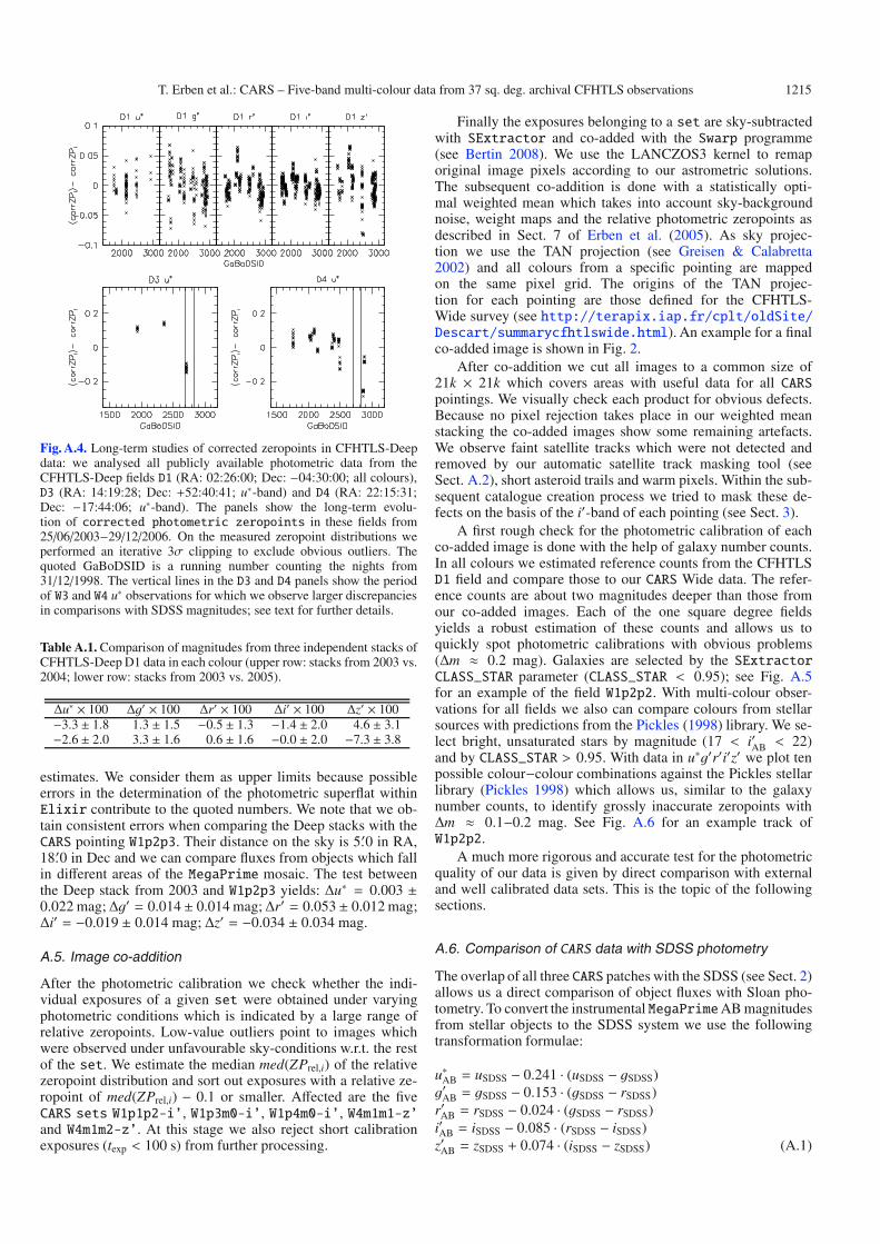
T. Erben et al.: CARS – Five-band multi-colour data from 37 sq. deg. archival CFHTLS observations 1215

Fig. A.4. Long-term studies of corrected zeropoints in CFHTLS-Deepdata: we analysed all publicly available photometric data from theCFHTLS-Deep fields D1 (RA: 02:26:00; Dec: −04:30:00; all colours),D3 (RA: 14:19:28; Dec: +52:40:41; u∗-band) and D4 (RA: 22:15:31;Dec: −17:44:06; u∗-band). The panels show the long-term evolu-tion of corrected photometric zeropoints in these fields from25/06/2003−29/12/2006. On the measured zeropoint distributions weperformed an iterative 3σ clipping to exclude obvious outliers. Thequoted GaBoDSID is a running number counting the nights from31/12/1998. The vertical lines in the D3 and D4 panels show the periodof W3 and W4 u∗ observations for which we observe larger discrepanciesin comparisons with SDSS magnitudes; see text for further details.

Table A.1. Comparison of magnitudes from three independent stacks ofCFHTLS-Deep D1 data in each colour (upper row: stacks from 2003 vs.2004; lower row: stacks from 2003 vs. 2005).

Δu∗ × 100 Δg′ × 100 Δr′ × 100 Δi′ × 100 Δz′ × 100−3.3 ± 1.8 1.3 ± 1.5 −0.5 ± 1.3 −1.4 ± 2.0 4.6 ± 3.1−2.6 ± 2.0 3.3 ± 1.6 0.6 ± 1.6 −0.0 ± 2.0 −7.3 ± 3.8

estimates. We consider them as upper limits because possibleerrors in the determination of the photometric superflat withinElixir contribute to the quoted numbers. We note that we ob-tain consistent errors when comparing the Deep stacks with theCARS pointing W1p2p3. Their distance on the sky is 5.′0 in RA,18.′0 in Dec and we can compare fluxes from objects which fallin different areas of the MegaPrime mosaic. The test betweenthe Deep stack from 2003 and W1p2p3 yields: Δu∗ = 0.003 ±0.022 mag;Δg′ = 0.014± 0.014 mag;Δr′ = 0.053± 0.012 mag;Δi′ = −0.019 ± 0.014 mag; Δz′ = −0.034 ± 0.034 mag.

A.5. Image co-addition

After the photometric calibration we check whether the indi-vidual exposures of a given set were obtained under varyingphotometric conditions which is indicated by a large range ofrelative zeropoints. Low-value outliers point to images whichwere observed under unfavourable sky-conditions w.r.t. the restof the set. We estimate the median med(ZPrel,i) of the relativezeropoint distribution and sort out exposures with a relative ze-ropoint of med(ZPrel,i) − 0.1 or smaller. Affected are the fiveCARS sets W1p1p2-i’, W1p3m0-i’, W1p4m0-i’, W4m1m1-z’and W4m1m2-z’. At this stage we also reject short calibrationexposures (texp < 100 s) from further processing.

Finally the exposures belonging to a set are sky-subtractedwith SExtractor and co-added with the Swarp programme(see Bertin 2008). We use the LANCZOS3 kernel to remaporiginal image pixels according to our astrometric solutions.The subsequent co-addition is done with a statistically opti-mal weighted mean which takes into account sky-backgroundnoise, weight maps and the relative photometric zeropoints asdescribed in Sect. 7 of Erben et al. (2005). As sky projec-tion we use the TAN projection (see Greisen & Calabretta2002) and all colours from a specific pointing are mappedon the same pixel grid. The origins of the TAN projec-tion for each pointing are those defined for the CFHTLS-Wide survey (see http://terapix.iap.fr/cplt/oldSite/Descart/summarycfhtlswide.html). An example for a finalco-added image is shown in Fig. 2.

After co-addition we cut all images to a common size of21k × 21k which covers areas with useful data for all CARSpointings. We visually check each product for obvious defects.Because no pixel rejection takes place in our weighted meanstacking the co-added images show some remaining artefacts.We observe faint satellite tracks which were not detected andremoved by our automatic satellite track masking tool (seeSect. A.2), short asteroid trails and warm pixels. Within the sub-sequent catalogue creation process we tried to mask these de-fects on the basis of the i′-band of each pointing (see Sect. 3).

A first rough check for the photometric calibration of eachco-added image is done with the help of galaxy number counts.In all colours we estimated reference counts from the CFHTLSD1 field and compare those to our CARS Wide data. The refer-ence counts are about two magnitudes deeper than those fromour co-added images. Each of the one square degree fieldsyields a robust estimation of these counts and allows us toquickly spot photometric calibrations with obvious problems(Δm ≈ 0.2 mag). Galaxies are selected by the SExtractorCLASS_STAR parameter (CLASS_STAR < 0.95); see Fig. A.5for an example of the field W1p2p2. With multi-colour obser-vations for all fields we also can compare colours from stellarsources with predictions from the Pickles (1998) library. We se-lect bright, unsaturated stars by magnitude (17 < i′AB < 22)and by CLASS_STAR > 0.95. With data in u∗g′r′i′z′ we plot tenpossible colour−colour combinations against the Pickles stellarlibrary (Pickles 1998) which allows us, similar to the galaxynumber counts, to identify grossly inaccurate zeropoints withΔm ≈ 0.1−0.2 mag. See Fig. A.6 for an example track ofW1p2p2.

A much more rigorous and accurate test for the photometricquality of our data is given by direct comparison with externaland well calibrated data sets. This is the topic of the followingsections.

A.6. Comparison of CARS data with SDSS photometry

The overlap of all three CARS patches with the SDSS (see Sect. 2)allows us a direct comparison of object fluxes with Sloan pho-tometry. To convert the instrumental MegaPrimeAB magnitudesfrom stellar objects to the SDSS system we use the followingtransformation formulae:

u∗AB = uSDSS − 0.241 · (uSDSS − gSDSS)g′AB = gSDSS − 0.153 · (gSDSS − rSDSS)r′AB = rSDSS − 0.024 · (gSDSS − rSDSS)i′AB = iSDSS − 0.085 · (rSDSS − iSDSS)z′AB = zSDSS + 0.074 · (iSDSS − zSDSS) (A.1)

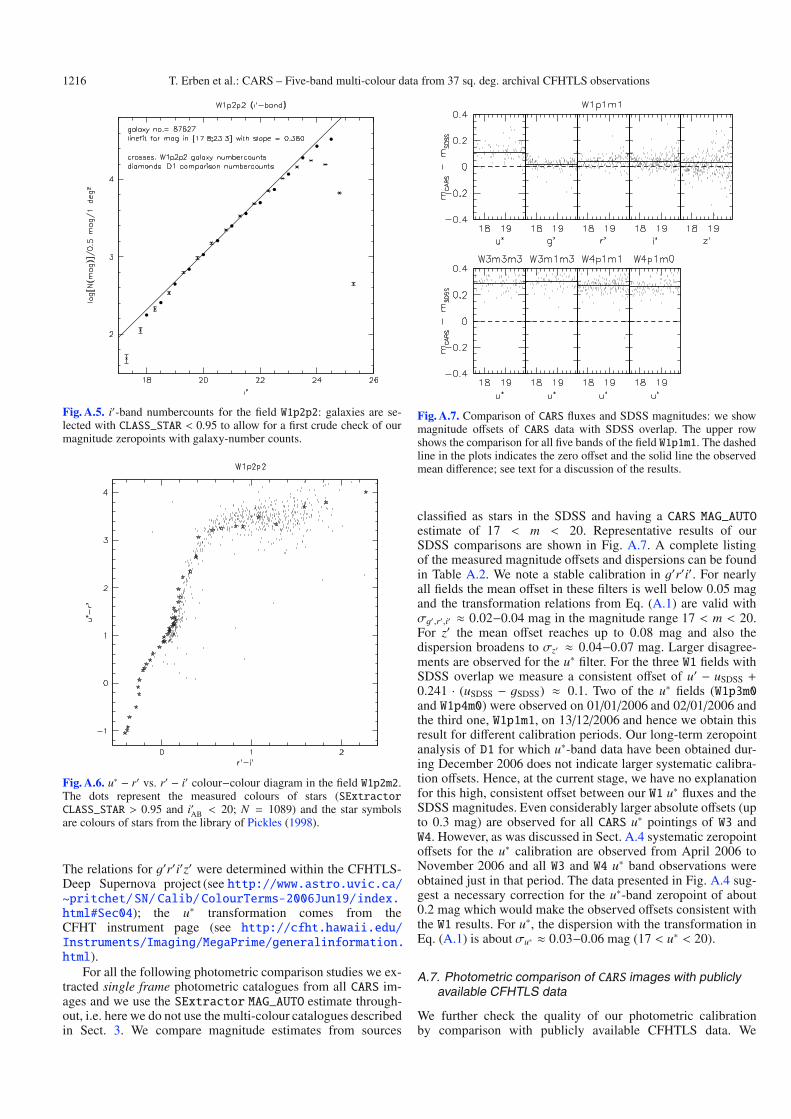
1216 T. Erben et al.: CARS – Five-band multi-colour data from 37 sq. deg. archival CFHTLS observations

Fig. A.5. i′-band numbercounts for the field W1p2p2: galaxies are se-lected with CLASS_STAR < 0.95 to allow for a first crude check of ourmagnitude zeropoints with galaxy-number counts.

Fig. A.6. u∗ − r′ vs. r′ − i′ colour−colour diagram in the field W1p2m2.The dots represent the measured colours of stars (SExtractorCLASS_STAR > 0.95 and i′AB < 20; N = 1089) and the star symbolsare colours of stars from the library of Pickles (1998).

The relations for g′r′i′z′ were determined within the CFHTLS-Deep Supernova project (see http://www.astro.uvic.ca/~pritchet/SN/ Calib/ColourTerms-2006Jun19/index.html#Sec04); the u∗ transformation comes from theCFHT instrument page (see http://cfht.hawaii.edu/Instruments/Imaging/MegaPrime/generalinformation.html).

For all the following photometric comparison studies we ex-tracted single frame photometric catalogues from all CARS im-ages and we use the SExtractor MAG_AUTO estimate through-out, i.e. here we do not use the multi-colour catalogues describedin Sect. 3. We compare magnitude estimates from sources

Fig. A.7. Comparison of CARS fluxes and SDSS magnitudes: we showmagnitude offsets of CARS data with SDSS overlap. The upper rowshows the comparison for all five bands of the field W1p1m1. The dashedline in the plots indicates the zero offset and the solid line the observedmean difference; see text for a discussion of the results.

classified as stars in the SDSS and having a CARS MAG_AUTOestimate of 17 < m < 20. Representative results of ourSDSS comparisons are shown in Fig. A.7. A complete listingof the measured magnitude offsets and dispersions can be foundin Table A.2. We note a stable calibration in g′r′i′. For nearlyall fields the mean offset in these filters is well below 0.05 magand the transformation relations from Eq. (A.1) are valid withσg′ ,r′,i′ ≈ 0.02−0.04 mag in the magnitude range 17 < m < 20.For z′ the mean offset reaches up to 0.08 mag and also thedispersion broadens to σz′ ≈ 0.04−0.07 mag. Larger disagree-ments are observed for the u∗ filter. For the three W1 fields withSDSS overlap we measure a consistent offset of u′ − uSDSS +0.241 · (uSDSS − gSDSS) ≈ 0.1. Two of the u∗ fields (W1p3m0and W1p4m0) were observed on 01/01/2006 and 02/01/2006 andthe third one, W1p1m1, on 13/12/2006 and hence we obtain thisresult for different calibration periods. Our long-term zeropointanalysis of D1 for which u∗-band data have been obtained dur-ing December 2006 does not indicate larger systematic calibra-tion offsets. Hence, at the current stage, we have no explanationfor this high, consistent offset between our W1 u∗ fluxes and theSDSS magnitudes. Even considerably larger absolute offsets (upto 0.3 mag) are observed for all CARS u∗ pointings of W3 andW4. However, as was discussed in Sect. A.4 systematic zeropointoffsets for the u∗ calibration are observed from April 2006 toNovember 2006 and all W3 and W4 u∗ band observations wereobtained just in that period. The data presented in Fig. A.4 sug-gest a necessary correction for the u∗-band zeropoint of about0.2 mag which would make the observed offsets consistent withthe W1 results. For u∗, the dispersion with the transformation inEq. (A.1) is about σu∗ ≈ 0.03−0.06 mag (17 < u∗ < 20).

A.7. Photometric comparison of CARS images with publiclyavailable CFHTLS data

We further check the quality of our photometric calibrationby comparison with publicly available CFHTLS data. We

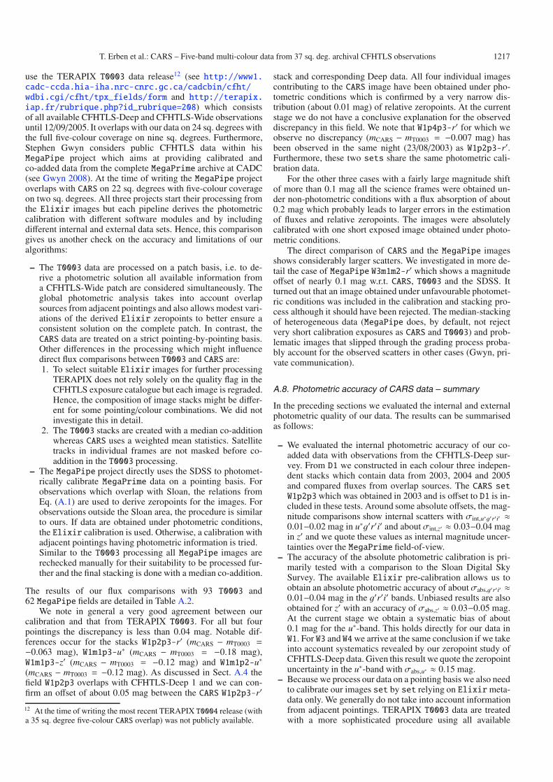
T. Erben et al.: CARS – Five-band multi-colour data from 37 sq. deg. archival CFHTLS observations 1217

use the TERAPIX T0003 data release12 (see http://www1.cadc-ccda.hia-iha.nrc-cnrc.gc.ca/cadcbin/cfht/wdbi.cgi/cfht/tpx_fields/form and http://terapix.iap.fr/rubrique.php?id_rubrique=208) which consistsof all available CFHTLS-Deep and CFHTLS-Wide observationsuntil 12/09/2005. It overlaps with our data on 24 sq. degrees withthe full five-colour coverage on nine sq. degrees. Furthermore,Stephen Gwyn considers public CFHTLS data within hisMegaPipe project which aims at providing calibrated andco-added data from the complete MegaPrime archive at CADC(see Gwyn 2008). At the time of writing the MegaPipe projectoverlaps with CARS on 22 sq. degrees with five-colour coverageon two sq. degrees. All three projects start their processing fromthe Elixir images but each pipeline derives the photometriccalibration with different software modules and by includingdifferent internal and external data sets. Hence, this comparisongives us another check on the accuracy and limitations of ouralgorithms:

– The T0003 data are processed on a patch basis, i.e. to de-rive a photometric solution all available information froma CFHTLS-Wide patch are considered simultaneously. Theglobal photometric analysis takes into account overlapsources from adjacent pointings and also allows modest vari-ations of the derived Elixir zeropoints to better ensure aconsistent solution on the complete patch. In contrast, theCARS data are treated on a strict pointing-by-pointing basis.Other differences in the processing which might influencedirect flux comparisons between T0003 and CARS are:1. To select suitable Elixir images for further processing

TERAPIX does not rely solely on the quality flag in theCFHTLS exposure catalogue but each image is regraded.Hence, the composition of image stacks might be differ-ent for some pointing/colour combinations. We did notinvestigate this in detail.

2. The T0003 stacks are created with a median co-additionwhereas CARS uses a weighted mean statistics. Satellitetracks in individual frames are not masked before co-addition in the T0003 processing.

– The MegaPipe project directly uses the SDSS to photomet-rically calibrate MegaPrime data on a pointing basis. Forobservations which overlap with Sloan, the relations fromEq. (A.1) are used to derive zeropoints for the images. Forobservations outside the Sloan area, the procedure is similarto ours. If data are obtained under photometric conditions,the Elixir calibration is used. Otherwise, a calibration withadjacent pointings having photometric information is tried.Similar to the T0003 processing all MegaPipe images arerechecked manually for their suitability to be processed fur-ther and the final stacking is done with a median co-addition.

The results of our flux comparisons with 93 T0003 and62 MegaPipe fields are detailed in Table A.2.

We note in general a very good agreement between ourcalibration and that from TERAPIX T0003. For all but fourpointings the discrepancy is less than 0.04 mag. Notable dif-ferences occur for the stacks W1p2p3-r′ (mCARS − mT0003 =−0.063 mag), W1m1p3-u∗ (mCARS − mT0003 = −0.18 mag),W1m1p3-z′ (mCARS − mT0003 = −0.12 mag) and W1m1p2-u∗(mCARS − mT0003 = −0.12 mag). As discussed in Sect. A.4 thefield W1p2p3 overlaps with CFHTLS-Deep 1 and we can con-firm an offset of about 0.05 mag between the CARS W1p2p3-r′

12 At the time of writing the most recent TERAPIX T0004 release (witha 35 sq. degree five-colour CARS overlap) was not publicly available.

stack and corresponding Deep data. All four individual imagescontributing to the CARS image have been obtained under pho-tometric conditions which is confirmed by a very narrow dis-tribution (about 0.01 mag) of relative zeropoints. At the currentstage we do not have a conclusive explanation for the observeddiscrepancy in this field. We note that W1p4p3-r′ for which weobserve no discrepancy (mCARS − mT0003 = −0.007 mag) hasbeen observed in the same night (23/08/2003) as W1p2p3-r′.Furthermore, these two sets share the same photometric cali-bration data.

For the other three cases with a fairly large magnitude shiftof more than 0.1 mag all the science frames were obtained un-der non-photometric conditions with a flux absorption of about0.2 mag which probably leads to larger errors in the estimationof fluxes and relative zeropoints. The images were absolutelycalibrated with one short exposed image obtained under photo-metric conditions.

The direct comparison of CARS and the MegaPipe imagesshows considerably larger scatters. We investigated in more de-tail the case of MegaPipe W3m1m2-r′ which shows a magnitudeoffset of nearly 0.1 mag w.r.t. CARS, T0003 and the SDSS. Itturned out that an image obtained under unfavourable photomet-ric conditions was included in the calibration and stacking pro-cess although it should have been rejected. The median-stackingof heterogeneous data (MegaPipe does, by default, not rejectvery short calibration exposures as CARS and T0003) and prob-lematic images that slipped through the grading process proba-bly account for the observed scatters in other cases (Gwyn, pri-vate communication).

A.8. Photometric accuracy of CARS data – summary

In the preceding sections we evaluated the internal and externalphotometric quality of our data. The results can be summarisedas follows:

– We evaluated the internal photometric accuracy of our co-added data with observations from the CFHTLS-Deep sur-vey. From D1 we constructed in each colour three indepen-dent stacks which contain data from 2003, 2004 and 2005and compared fluxes from overlap sources. The CARS setW1p2p3which was obtained in 2003 and is offset to D1 is in-cluded in these tests. Around some absolute offsets, the mag-nitude comparisons show internal scatters with σint,u∗g′r′i′ ≈0.01−0.02 mag in u∗g′r′i′ and about σint,z′ ≈ 0.03−0.04 magin z′ and we quote these values as internal magnitude uncer-tainties over the MegaPrime field-of-view.

– The accuracy of the absolute photometric calibration is pri-marily tested with a comparison to the Sloan Digital SkySurvey. The available Elixir pre-calibration allows us toobtain an absolute photometric accuracy of about σabs,g′r′i′ ≈0.01−0.04 mag in the g′r′i′ bands. Unbiased results are alsoobtained for z′ with an accuracy of σabs,z′ ≈ 0.03−0.05 mag.At the current stage we obtain a systematic bias of about0.1 mag for the u∗-band. This holds directly for our data inW1. For W3 and W4we arrive at the same conclusion if we takeinto account systematics revealed by our zeropoint study ofCFHTLS-Deep data. Given this result we quote the zeropointuncertainty in the u∗-band with σabs,u∗ ≈ 0.15 mag.

– Because we process our data on a pointing basis we also needto calibrate our images set by set relying on Elixirmeta-data only. We generally do not take into account informationfrom adjacent pointings. TERAPIX T0003 data are treatedwith a more sophisticated procedure using all available

1218 T. Erben et al.: CARS – Five-band multi-colour data from 37 sq. deg. archival CFHTLS observations

Table A.2. CARS data quality overview; see the text for details.

Field/Areaa Filter N expos. time mlim Sloanb T3/MegaP.c seeing comments[sq. deg.] [s] [AB mag] Δm × 100 Δm × 100 [′′]W1m0p1 u∗ 5 3000.51 25.27 – 0.0 ± 0.8 (T) 1.00[w1.−0+1] −0.4 ± 1.3 (M)(0.84) g′ 5 2500.45 25.55 – −0.4 ± 0.5 (T) 0.90

−7.1 ± 0.9 (M)r′ 3 1500.28 24.72 – −1.9 ± 1.0 (T) 0.79i′ 7 4305.67 24.61 – −0.1 ± 0.8 (T) 0.85

−0.8 ± 0.7 (M)z′ 11 6601.19 23.88 – 0.2 ± 1.5 (T) 0.79

−7.7 ± 1.1 (M)W1m0p2 u∗ 5 3000.58 25.35 – −0.6 ± 1.1 (T) 1.00[w1.−0+2] −2.2 ± 1.5 (M)(0.76) g′ 7 3500.46 25.72 – −0.5 ± 1.0 (T) 0.95

−2.5 ± 0.9 (M)r′ 2 1000.18 24.61 – −0.5 ± 0.5 (T) 0.82 no ch. 21, 35i′ 7 4305.66 24.72 – 1.3 ± 2.4 (T) 0.74

0.2 ± 1.8 (M)z′ 10 6000.83 23.64 – −1.2 ± 3.5 (T) 0.79 fr. res.

−7.3 ± 1.5 (M)W1m0p3 u∗ 5 3000.58 25.27 – −1.0 ± 1.4 (T) 0.87[w1.−0+3] 5.3 ± 1.2 (M)(0.75) g′ 5 2500.49 25.56 – −0.7 ± 0.8 (T) 0.90

−1.9 ± 0.6 (M)r′ 2 1000.18 24.62 – −1.2 ± 0.5 (T) 0.85 no ch. 21, 35i′ 7 4305.65 24.59 – −0.5 ± 0.7 (T) 0.74

−0.8 ± 0.5 (M)z′ 10 6000.84 23.59 – −1.3 ± 2.7 (T) 0.82 fr. res.

−8.1 ± 1.4 (M)W1m1p1 u∗ 7 4200.60 25.50 – – 1.00[w1.−1+1] g′ 8 4000.76 25.73 – – 0.66(0.84) r′ 2 1000.20 24.51 – – 0.59

i′ 9 5535.73 24.53 – – 0.79z′ 6 3600.40 23.30 – – 0.75

W1m1p2 u∗ 5 3000.52 25.03 – −12.0 ± 0.6 (T) 0.92[w1.−1+2] −9.2 ± 1.5 (M)(0.82) g′ 5 2500.48 25.44 – 3.3 ± 0.7 (T) 0.87

−4.1 ± 1.0 (M)r′ 4 2000.38 24.80 – 1.0 ± 2.2 (T) 0.87

−2.1 ± 2.0 (M)i′ 7 4305.66 24.52 – −0.1 ± 1.8 (T) 0.71

1.6 ± 2.1 (M)z′ 11 6601.18 23.87 – −1.1 ± 1.5 (T) 0.71 fr. res.

0.3 ± 0.8 (M)W1m1p3 u∗ 5 3000.50 24.95 – −18.3 ± 0.5 (T) 0.79[w1.−1+3] g′ 3 1500.30 25.22 – 1.0 ± 0.8 (T) 0.77(0.76) r′ 2 1000.23 24.58 – 1.4 ± 0.8 (T) 0.79 no ch. 21, 35

i′ 7 4305.70 24.58 – −0.3 ± 1.0 (T) 0.74z′ 10 6001.00 23.43 – −11.9 ± 2.3 (T) 0.71 fr. res.

W1p1m1 u∗ 5 3000.42 25.26 12.2 ± 5.5 – 0.85[w1.+1−1] g′ 6 3000.47 25.79 2.7 ± 2.8 – 0.87(0.85) r′ 2 1000.16 24.50 4.2 ± 3.4 – 0.71

i′ 7 4305.53 24.85 5.2 ± 4.8 – 0.71z′ 6 3600.40 23.52 1.3 ± 5.7 – 0.85

W1p1p1 u∗ 5 3000.47 25.28 – 0.6 ± 0.9 (T) 0.92[w1.+1+1] 6.6 ± 0.7 (M)(0.75) g′ 10 5000.88 25.97 – −0.3 ± 0.7 (T) 0.95

−2.0 ± 0.5 (M)r′ 2 1000.18 24.57 – −1.6 ± 0.6 (T) 0.85i′ 7 4305.72 24.70 – −0.1 ± 0.8 (T) 0.82

−0.5 ± 0.5 (M)z′ 12 7201.21 23.94 – 0.9 ± 1.5 (T) 0.74 fr. res.

−9.3 ± 1.3 (M)

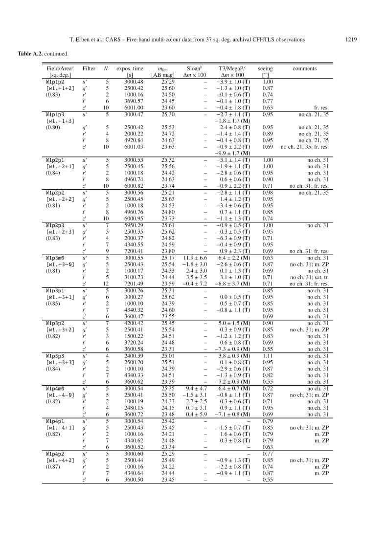
T. Erben et al.: CARS – Five-band multi-colour data from 37 sq. deg. archival CFHTLS observations 1219

Table A.2. continued.

Field/Areaa Filter N expos. time mlim Sloanb T3/MegaP.c seeing comments[sq. deg.] [s] [AB mag] Δm × 100 Δm × 100 [′′]W1p1p2 u∗ 5 3000.48 25.29 – −3.9 ± 1.0 (T) 1.00[w1.+1+2] g′ 5 2500.42 25.60 – −1.3 ± 1.0 (T) 0.87(0.83) r′ 2 1000.16 24.50 – −0.1 ± 0.6 (T) 0.74

i′ 6 3690.57 24.45 – −0.1 ± 1.0 (T) 0.77z′ 10 6001.00 23.60 – −0.4 ± 1.8 (T) 0.63 fr. res.

W1p1p3 u∗ 5 3000.47 25.30 – −2.7 ± 1.1 (T) 0.95 no ch. 21, 35[w1.+1+3] −1.8 ± 1.7 (M)(0.80) g′ 5 2500.42 25.53 – 2.4 ± 0.8 (T) 0.95 no ch. 21, 35

r′ 4 2000.22 24.72 – −1.4 ± 1.4 (T) 0.89 no ch. 21, 35i′ 8 4920.84 24.63 – −0.4 ± 0.8 (T) 0.95 no ch. 21, 35z′ 10 6001.03 23.63 – −0.9 ± 2.2 (T) 0.69 no ch. 21, 35; fr. res.

−9.9 ± 1.7 (M)W1p2p1 u∗ 5 3000.53 25.32 – −3.1 ± 1.4 (T) 1.00 no ch. 31[w1.+2+1] g′ 5 2500.45 25.56 – −1.9 ± 1.1 (T) 1.00 no ch. 31(0.84) r′ 2 1000.18 24.42 – −2.8 ± 0.6 (T) 0.95 no ch. 31

i′ 8 4960.74 24.63 – 0.6 ± 0.6 (T) 0.90 no ch. 31z′ 10 6000.82 23.74 – −0.9 ± 2.2 (T) 0.71 no ch. 31; fr. res.

W1p2p2 u∗ 5 3000.56 25.21 – −2.8 ± 1.1 (T) 0.98 no ch. 21, 35[w1.+2+2] g′ 5 2500.45 25.63 – 1.4 ± 1.2 (T) 0.95(0.81) r′ 2 1000.18 24.53 – −3.4 ± 0.6 (T) 0.95

i′ 8 4960.76 24.80 – 0.7 ± 1.1 (T) 0.85z′ 10 6000.95 23.73 – −1.1 ± 1.3 (T) 0.74

W1p2p3 u∗ 7 5950.29 25.61 – −0.9 ± 0.5 (T) 1.00 no ch. 31[w1.+2+3] g′ 5 2500.35 25.62 – −0.3 ± 0.5 (T) 0.95(0.83) r′ 4 2000.37 24.82 – −6.3 ± 0.9 (T) 0.71

i′ 7 4340.55 24.59 – −0.4 ± 0.9 (T) 0.95z′ 9 7200.41 23.80 – 0.9 ± 2.3 (T) 0.69 no ch. 31; fr. res.

W1p3m0 u∗ 5 3000.55 25.17 11.9 ± 6.6 6.4 ± 2.2 (M) 0.63 no ch. 31[w1.+3−0] g′ 5 2500.43 25.54 −1.8 ± 3.0 −2.6 ± 0.6 (T) 0.87 no ch. 31; m. ZP(0.81) r′ 2 1000.17 24.33 2.4 ± 3.0 0.1 ± 1.3 (T) 0.69 no ch. 31

i′ 5 3100.23 24.44 3.5 ± 3.5 3.1 ± 1.0 (T) 0.71 no ch. 31; sat. tr.z′ 12 7201.49 23.59 −0.4 ± 7.2 −8.8 ± 3.7 (M) 0.71 no ch. 31; fr. res.

W1p3p1 u∗ 5 3000.26 25.31 – – 0.85 no ch. 31[w1.+3+1] g′ 6 3000.27 25.62 – 0.0 ± 0.5 (T) 0.95 no ch. 31(0.85) r′ 2 1000.10 24.39 – 0.5 ± 0.7 (T) 0.85 no ch. 31

i′ 7 4340.32 24.60 – −0.8 ± 1.1 (T) 0.95 no ch. 31z′ 6 3600.47 23.55 – – 0.69 no ch. 31

W1p3p2 u∗ 7 4200.42 25.45 – 5.0 ± 1.5 (M) 0.90 no ch. 31[w1.+3+2] g′ 5 2500.41 25.54 – 0.3 ± 0.9 (T) 0.85 no ch. 31; m. ZP(0.82) r′ 3 1500.22 24.51 – −1.2 ± 1.2 (T) 0.83 no ch. 31

i′ 6 3720.24 24.48 – 0.6 ± 0.8 (T) 0.69 no ch. 31z′ 6 3600.58 23.31 – −7.3 ± 0.9 (M) 0.55 no ch. 31

W1p3p3 u∗ 4 2400.39 25.01 – 3.8 ± 0.9 (M) 1.11 no ch. 31[w1.+3+3] g′ 5 2500.20 25.51 – 0.1 ± 0.8 (T) 0.95 no ch. 31(0.84) r′ 2 1000.10 24.39 – −2.9 ± 0.6 (T) 0.87 no ch. 31

i′ 7 4340.33 24.51 – −1.3 ± 0.9 (T) 0.82 no ch. 31z′ 6 3600.62 23.39 – −7.2 ± 0.9 (M) 0.55 no ch. 31

W1p4m0 u∗ 5 3000.54 25.35 9.4 ± 4.7 6.4 ± 0.7 (M) 0.72 no ch. 31[w1.+4−0] g′ 5 2500.41 25.50 −1.5 ± 3.1 −0.8 ± 1.1 (T) 0.87 no ch. 31; m. ZP(0.82) r′ 2 1000.19 24.33 2.7 ± 2.5 0.3 ± 0.6 (T) 0.71 no ch. 31

i′ 4 2480.15 24.15 0.1 ± 3.1 0.9 ± 1.1 (T) 0.95 no ch. 31z′ 6 3600.72 23.48 0.4 ± 5.9 −7.1 ± 0.8 (M) 0.69 no ch. 31

W1p4p1 u∗ 5 3000.54 25.42 – – 0.79[w1.+4+1] g′ 5 2500.43 25.45 – −1.5 ± 0.7 (T) 0.85 no ch. 31; m. ZP(0.82) r′ 2 1000.16 24.21 – 1.6 ± 0.6 (T) 0.79 m. ZP

i′ 7 4340.62 24.48 – 0.3 ± 0.8 (T) 0.79 m. ZPz′ 6 3600.52 23.34 – – 0.63

W1p4p2 u∗ 5 3000.60 25.29 – – 0.77[w1.+4+2] g′ 5 2500.44 25.49 – −0.9 ± 1.3 (T) 0.85 no ch. 31; m. ZP(0.87) r′ 2 1000.16 24.22 – −2.2 ± 0.8 (T) 0.74 m. ZP

i′ 7 4340.64 24.44 – −0.9 ± 1.1 (T) 0.87 m. ZPz′ 6 3600.50 23.45 – – 0.55

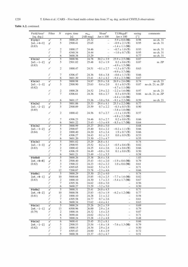
1220 T. Erben et al.: CARS – Five-band multi-colour data from 37 sq. deg. archival CFHTLS observations

Table A.2. continued.

Field/Areaa Filter N expos. time mlim Sloanb T3/MegaP.c seeing comments[sq. deg.] [s] [AB mag] Δm × 100 Δm × 100 [′′]W1p4p3 u∗ 5 3000.25 25.32 – 5.9 ± 0.8 (M) 0.98 no ch. 31[w1.+4+3] g′ 5 2500.41 25.65 – −0.9 ± 2.3 (T) 0.95 no ch. 31(0.83) −1.4 ± 1.1 (M)

r′ 2 1000.17 24.46 – −0.7 ± 1.0 (T) 0.93 no ch. 31i′ 7 4340.34 24.44 – −1.0 ± 0.7 (T) 0.95 no ch. 31z′ 6 3600.38 23.29 – – 0.77 no ch. 31

W3m1m2 u∗ 5 3000.96 24.78 30.2 ± 3.9 25.9 ± 2.5 (M) 0.87[w3.−1−2] g′ 5 2501.02 25.48 0.2 ± 1.9 0.2 ± 0.6 (T) 0.87 m. ZP(0.83) −4.9 ± 1.5 (M)

r′ 2 1000.47 24.51 −0.1 ± 2.7 −1.3 ± 0.7 (T) 0.63−9.9 ± 3.7 (M)

i′ 7 4306.47 24.36 0.6 ± 3.8 −0.6 ± 1.3 (T) 0.66z′ 6 3601.20 23.41 −6.1 ± 4.2 −9.4 ± 2.3 (M) 0.67

W3m1m3 u∗ 5 3000.98 24.87 29.9 ± 3.8 26.9 ± 2.6 (M) 0.74 no ch. 21[w3.−1−3] g′ 5 2500.90 25.63 0.4 ± 2.0 0.1 ± 0.5 (T) 0.87 no ch. 21; m. ZP(0.82) −4.7 ± 1.1 (M)

r′ 2 1000.28 24.52 2.9 ± 2.2 −2.2 ± 1.6 (M) 0.97 no ch. 21i′ 7 4306.61 24.36 0.6 ± 2.7 0.3 ± 0.9 (T) 0.66 no ch. 21; m. ZP

−4.4 ± 1.6 (M)z′ 6 3601.17 23.36 −3.8 ± 5.6 −9.1 ± 2.2 (M) 0.59 no ch. 21

W3m2m2 u∗ 5 3001.06 25.33 29.4 ± 4.1 25.3 ± 2.2 (M) 0.77[w3.−2−2] g′ 5 2500.89 25.59 0.7 ± 2.2 −0.3 ± 0.5 (T) 0.90(0.85) −3.8 ± 1.0 (M)

r′ 2 1000.42 24.56 0.7 ± 2.7 −1.1 ± 1.0 (T) 0.57−4.8 ± 2.2 (M)

i′ 7 4306.23 24.46 0.3 ± 2.7 0.2 ± 0.8 (T) 0.66z′ 6 3601.22 23.43 −3.3 ± 4.9 −8.5 ± 1.7 (M) 0.64

W3m3m2 u∗ 5 3000.99 25.27 29.0 ± 5.0 – 0.68[w3.−3−2] g′ 5 2500.87 25.40 0.4 ± 2.2 −0.2 ± 1.1 (T) 0.66(0.84) r′ 2 1000.40 24.20 4.5 ± 2.4 1.9 ± 0.7 (T) 0.66

i′ 7 4306.27 24.43 0.1 ± 3.3 0.0 ± 0.9 (T) 0.53z′ 6 3601.20 23.30 −2.3 ± 4.7 – 0.55

W3m3m3 u∗ 5 3001.02 25.29 28.8 ± 4.1 – 0.74[w3.−3−3] g′ 5 2500.93 25.52 0.2 ± 2.3 −0.5 ± 0.6 (T) 0.82(0.83) r′ 2 1000.42 24.25 4.4 ± 2.6 1.4 ± 0.6 (T) 0.66

i′ 7 4306.19 24.49 −0.8 ± 3.0 0.1 ± 0.8 (T) 0.50z′ 6 3601.21 23.49 −3.1 ± 5.5 - 0.58

W4m0m0 u∗ 5 3000.26 25.38 26.4 ± 3.8 – 1.03[w4.+0+0] g′ 5 2500.40 25.43 −0.1 ± 2.0 −1.9 ± 0.6 (M) 0.79(0.82) r′ 3 1500.22 24.23 −0.2 ± 2.2 1.0 ± 0.6 (M) 0.61

i′ 7 4305.65 24.62 5.3 ± 3.3 – 0.71z′ 12 7200.87 23.78 −2.3 ± 4.6 – 0.66

W4m0m1 u∗ 5 3000.29 25.30 23.2 ± 4.0 – 0.74[w4.+0−1] g′ 10 5000.68 25.85 −0.2 ± 2.5 −7.7 ± 1.6 (M) 0.82(0.83) r′ 2 1000.10 24.30 1.7 ± 2.3 −5.4 ± 1.7 (M) 0.67

i′ 7 4305.36 24.62 −0.8 ± 3.0 – 0.56z′ 6 3600.27 23.29 −3.2 ± 5.0 – 0.50

W4m0m2 u∗ 5 3000.31 25.41 24.0 ± 4.5 – 0.71[w4.+0−2] g′ 10 5000.58 25.83 −0.3 ± 1.9 −6.2 ± 1.2 (M) 0.77(0.81) r′ 2 1000.10 24.28 2.1 ± 2.2 – 0.58

i′ 7 4305.58 24.77 0.7 ± 2.6 – 0.61z′ 6 3600.34 23.62 −4.4 ± 4.1 – 0.63

W4m1m1 u∗ 5 3000.24 25.26 24.2 ± 3.9 – 0.69[w4.−1−1] g′ 13 6500.96 26.00 2.9 ± 2.4 – 0.79(0.79) r′ 2 1000.16 24.32 1.4 ± 2.5 – 0.87

i′ 6 3690.44 24.62 −0.2 ± 3.2 – 0.71z′ 5 3000.24 23.28 −1.2 ± 4.8 – 0.48

W4m1m2 u∗ 6 3600.41 25.45 33.2 ± 8.1 – 0.66[w4.−1−2] g′ 5 2500.53 25.54 −1.8 ± 1.8 −7.6 ± 1.3 (M) 0.79(0.82) r′ 2 1000.15 24.34 2.9 ± 2.4 – 0.50

i′ 7 4305.43 24.60 1.8 ± 2.9 – 0.72z′ 5 3000.38 23.37 −0.3 ± 4.7 – 0.51

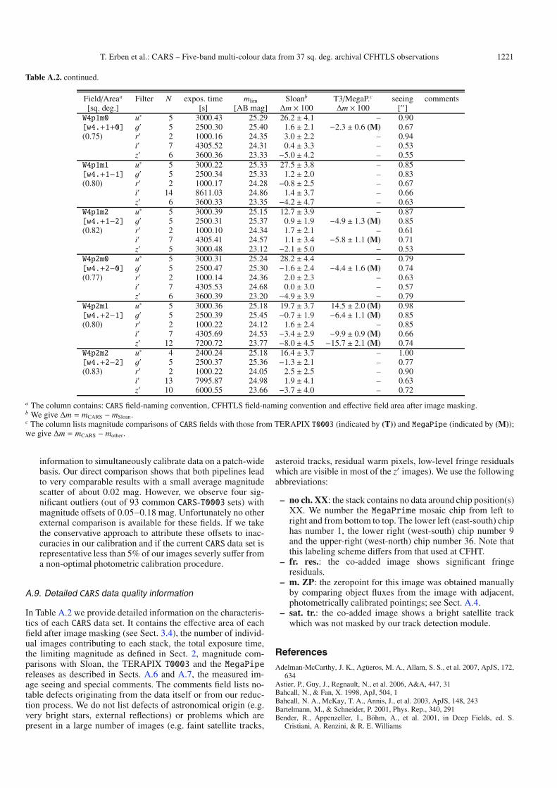
T. Erben et al.: CARS – Five-band multi-colour data from 37 sq. deg. archival CFHTLS observations 1221

Table A.2. continued.

Field/Areaa Filter N expos. time mlim Sloanb T3/MegaP.c seeing comments[sq. deg.] [s] [AB mag] Δm × 100 Δm × 100 [′′]W4p1m0 u∗ 5 3000.43 25.29 26.2 ± 4.1 – 0.90[w4.+1+0] g′ 5 2500.30 25.40 1.6 ± 2.1 −2.3 ± 0.6 (M) 0.67(0.75) r′ 2 1000.16 24.35 3.0 ± 2.2 – 0.94

i′ 7 4305.52 24.31 0.4 ± 3.3 – 0.53z′ 6 3600.36 23.33 −5.0 ± 4.2 – 0.55

W4p1m1 u∗ 5 3000.22 25.33 27.5 ± 3.8 – 0.85[w4.+1−1] g′ 5 2500.34 25.33 1.2 ± 2.0 – 0.83(0.80) r′ 2 1000.17 24.28 −0.8 ± 2.5 – 0.67

i′ 14 8611.03 24.86 1.4 ± 3.7 – 0.66z′ 6 3600.33 23.35 −4.2 ± 4.7 – 0.63

W4p1m2 u∗ 5 3000.39 25.15 12.7 ± 3.9 – 0.87[w4.+1−2] g′ 5 2500.31 25.37 0.9 ± 1.9 −4.9 ± 1.3 (M) 0.85(0.82) r′ 2 1000.10 24.34 1.7 ± 2.1 – 0.61

i′ 7 4305.41 24.57 1.1 ± 3.4 −5.8 ± 1.1 (M) 0.71z′ 5 3000.48 23.12 −2.1 ± 5.0 – 0.53

W4p2m0 u∗ 5 3000.31 25.24 28.2 ± 4.4 – 0.79[w4.+2−0] g′ 5 2500.47 25.30 −1.6 ± 2.4 −4.4 ± 1.6 (M) 0.74(0.77) r′ 2 1000.14 24.36 2.0 ± 2.3 – 0.63

i′ 7 4305.53 24.68 0.0 ± 3.0 – 0.57z′ 6 3600.39 23.20 −4.9 ± 3.9 – 0.79

W4p2m1 u∗ 5 3000.36 25.18 19.7 ± 3.7 14.5 ± 2.0 (M) 0.98[w4.+2−1] g′ 5 2500.39 25.45 −0.7 ± 1.9 −6.4 ± 1.1 (M) 0.85(0.80) r′ 2 1000.22 24.12 1.6 ± 2.4 – 0.85

i′ 7 4305.69 24.53 −3.4 ± 2.9 −9.9 ± 0.9 (M) 0.66z′ 12 7200.72 23.77 −8.0 ± 4.5 −15.7 ± 2.1 (M) 0.74

W4p2m2 u∗ 4 2400.24 25.18 16.4 ± 3.7 – 1.00[w4.+2−2] g′ 5 2500.37 25.36 −1.3 ± 2.1 – 0.77(0.83) r′ 2 1000.22 24.05 2.5 ± 2.5 – 0.90

i′ 13 7995.87 24.98 1.9 ± 4.1 – 0.63z′ 10 6000.55 23.66 −3.7 ± 4.0 – 0.72

a The column contains: CARS field-naming convention, CFHTLS field-naming convention and effective field area after image masking.b We give Δm = mCARS − mSloan.c The column lists magnitude comparisons of CARS fields with those from TERAPIX T0003 (indicated by (T)) and MegaPipe (indicated by (M));we give Δm = mCARS − mother.

information to simultaneously calibrate data on a patch-widebasis. Our direct comparison shows that both pipelines leadto very comparable results with a small average magnitudescatter of about 0.02 mag. However, we observe four sig-nificant outliers (out of 93 common CARS-T0003 sets) withmagnitude offsets of 0.05−0.18 mag. Unfortunately no otherexternal comparison is available for these fields. If we takethe conservative approach to attribute these offsets to inac-curacies in our calibration and if the current CARS data set isrepresentative less than 5% of our images severly suffer froma non-optimal photometric calibration procedure.

A.9. Detailed CARS data quality information

In Table A.2 we provide detailed information on the characteris-tics of each CARS data set. It contains the effective area of eachfield after image masking (see Sect. 3.4), the number of individ-ual images contributing to each stack, the total exposure time,the limiting magnitude as defined in Sect. 2, magnitude com-parisons with Sloan, the TERAPIX T0003 and the MegaPipereleases as described in Sects. A.6 and A.7, the measured im-age seeing and special comments. The comments field lists no-table defects originating from the data itself or from our reduc-tion process. We do not list defects of astronomical origin (e.g.very bright stars, external reflections) or problems which arepresent in a large number of images (e.g. faint satellite tracks,

asteroid tracks, residual warm pixels, low-level fringe residualswhich are visible in most of the z′ images). We use the followingabbreviations:

– no ch. XX: the stack contains no data around chip position(s)XX. We number the MegaPrime mosaic chip from left toright and from bottom to top. The lower left (east-south) chiphas number 1, the lower right (west-south) chip number 9and the upper-right (west-north) chip number 36. Note thatthis labeling scheme differs from that used at CFHT.

– fr. res.: the co-added image shows significant fringeresiduals.

– m. ZP: the zeropoint for this image was obtained manuallyby comparing object fluxes from the image with adjacent,photometrically calibrated pointings; see Sect. A.4.

– sat. tr.: the co-added image shows a bright satellite trackwhich was not masked by our track detection module.

ReferencesAdelman-McCarthy, J. K., Agüeros, M. A., Allam, S. S., et al. 2007, ApJS, 172,

634Astier, P., Guy, J., Regnault, N., et al. 2006, A&A, 447, 31Bahcall, N., & Fan, X. 1998, ApJ, 504, 1Bahcall, N. A., McKay, T. A., Annis, J., et al. 2003, ApJS, 148, 243Bartelmann, M., & Schneider, P. 2001, Phys. Rep., 340, 291Bender, R., Appenzeller, I., Böhm, A., et al. 2001, in Deep Fields, ed. S.

Cristiani, A. Renzini, & R. E. Williams

1222 T. Erben et al.: CARS – Five-band multi-colour data from 37 sq. deg. archival CFHTLS observations

Benitez, N. 2000, ApJ, 536, 571Bertin, E. 2003, SExtractor v2.3 User’s manual, http://terapix.iap.fr/Bertin, E. 2008, Swarp v2.17.0 User’s guide, http://terapix.iap.fr/Bertin, E., & Arnouts, S. 1996, A&AS, 117, 393Bertin, E., & Marmo, C. 2007, Weightwatcher v1.8.6 User’s guidehttp://terapix.iap.fr/

Böhringer, H., Voges, W., Huchra, J. P., et al. 2000, ApJS, 129, 435Böhringer, H., Schuecker, P., Guzzo, L., et al. 2004, A&A, 425, 367Bolzonella, M., Miralles, J. M., & Pelló, R. 2000, A&A, 363, 476Borgani, S., & Guzzo, L. 2001, Nature, 409, 39Borgani, S., Rosati, P., Tozzi, P., & Norman, C. 1999, ApJ, 517, 40Boulade, O., Charlot, X., Abbon, P., et al. 2003, in Instrument Design and

Performance for Optical/Infrared Ground-based Telescopes, ed. M. Iye, &A. F. M. Moorwood, Proc. SPIE, 4841, 72

Brimioulle, F., Lerchster, M., Seitz, S., Bender, R., & Snigula, J. 2008[arXiv:0811.3211]

Coleman, G. D., Wu, C.-C., & Weedman, D. W. 1980, ApJS, 43, 393Coupon, J., Ilbert, O., Kilbinger, M., et al. 2008 [arXiv:0811.3326]Dahle, H., Pedersen, K., Lilje, P. B., Maddox, S. J., & Kaiser, N. 2003, ApJ, 591,

662Davis, M., Guhathakurta, P., Konidaris, N. P., et al. 2007, ApJ, 660, L1Dietrich, J. P., Erben, T., Lamer, G., et al. 2007, A&A, 470, 821Duda, R. O., & Hart, P. E. 1972, Commun. ACM, 15, 11Eke, V. R., Cole, S., & Frenk, C. S. 1996, MNRAS, 282, 263Erben, T., van Waerbeke, L., Mellier, Y., et al. 2000, A&A, 355, 23Erben, T., Schirmer, M., Dietrich, J. P., et al. 2005, Astron. Nachr., 326, 432Feldmann, R., Carollo, C. M., Porciani, C., et al. 2006, MNRAS, 372, 565Fu, L., Semboloni, E., Hoekstra, H., et al. 2008, A&A, 479, 9Gal, R. R. 2008, in Lecture Notes in Physics (Berlin, Heidelberg: Springer), 740,

119Garilli, B., Le Fèvre, O., Guzzo, L., et al. 2008, A&A, 486, 683Gladders, M. D., & Yee, H. K. C. 2000, AJ, 120, 2148Gladders, M. D., Yee, H. K. C., Majumdar, S., et al. 2007, ApJ, 655, 128Goto, T., Sekiguchi, M., Nichol, R. C., et al. 2002, AJ, 123, 1807Greisen, E. W., & Calabretta, M. R. 2002, A&A, 395, 1061Gwyn, S. D. J. 2008, PASP, 120, 212Hetterscheidt, M., Erben, T., Schneider, P., et al. 2005, A&A, 442, 43Hildebrandt, H., Erben, T., Dietrich, J. P., et al. 2006, A&A, 452, 1121Hildebrandt, H., Wolf, C., & Benítez, N. 2008, A&A, 480, 703Hoekstra, H., Mellier, Y., van Waerbeke, L., et al. 2006, ApJ, 647, 116Huterer, D., Takada, M., Bernstein, G., & Jain, B. 2006, MNRAS, 366, 101Ilbert, O., Arnouts, S., McCracken, H. J., et al. 2006, A&A, 457, 841Kerscher, M., Szapudi, I., & Szalay, A. S. 2000, ApJ, 535, L13

Kinney, A. L., Calzetti, D., Bohlin, R. C., et al. 1996, ApJ, 467, 38Koch, A., Grebel, E., Odenkirchen, M., & Caldwell, J. A. R. 2004, AN, 325, 299Koester, B. P., McKay, T. A., Annis, J., et al. 2007, ApJ, 660, 239Landy, S. D., & Szalay, A. S. 1993, ApJ, 412, 64Le Fèvre, O., Vettolani, G., Garilli, B., et al. 2005, A&A, 439, 845Lilly, S. J., Le Fèvre, O., Crampton, D., Hammer, F., & Tresse, L. 1995, ApJ,

455, 50Magnier, E. A., & Cuillandre, J.-C. 2004, PASP, 116, 449Mandelbaum, R., Seljak, U., Hirata, C. M., et al. 2008, MNRAS, 386, 781Manfroid, J., Selman, F., & Jones, H. 2001, ESO Messenger, 102, 16Mantz, A., Allen, S. W., Ebeling, H., & Rapetti, D. 2008, MNRAS, 387, 1179Marmo, C., & Bertin, E. 2008, in Astronomical Data Analysis Software and

Systems XVII, ed. R. W. Argyle, P. S. Bunclark, & J. R. Lewis, ASP Conf.Ser., 394, 619

McCracken, H. J., Radovich, M., Bertin, E., et al. 2003, A&A, 410, 17Miller, C. J., Nichol, R. C., Reichart, D., et al. 2005, AJ, 130, 968Mobasher, B., Idzi, R., Benítez, N., et al. 2004, ApJ, 600, L167Monet, D. G., Levine, S. E., Canzian, B., et al. 2003, AJ, 125, 984Olsen, L. F., Scodeggio, M., da Costa, L., et al. 1999, A&A, 345, 681Olsen, L. F., Benoist, C., da Costa, L., et al. 2001, A&A, 380, 460Pickles, A. J. 1998, PASP, 110, 863Postman, M., Lubin, L. M., Gunn, J. E., et al. 1996, AJ, 111, 615Radovich, M. 2002, ASTROMETRIX User’s manualRamella, M., Boschin, W., Fadda, D., & Nonino, M. 2001, A&A, 368, 776Regnault, N. 2007, in The Future of Photometric, Spectrophotometric and

Polarimetric Standardization, ed. C. Sterken, ASP Conf. Ser., 364, 587Reiprich, T. H., & Böhringer, H. 2002, ApJ, 567, 716Schirmer, M., Erben, T., Schneider, P., et al. 2003, A&A, 407, 869Schirmer, M., Erben, T., Hetterscheidt, M., & Schneider, P. 2007, A&A, 462,

875Schneider, P. 1996, MNRAS, 283, 837Schneider, M., Knox, L., Zhan, H., & Connolly, A. 2006, ApJ, 651, 14Schuecker, P., Böhringer, H., Collins, C. A., & Guzzo, L. 2003a, A&A, 398,

867Schuecker, P., Caldwell, R. R., Böhringer, H., et al. 2003b, A&A, 402, 53van Waerbeke, L., White, M., Hoekstra, H., & Heymans, C. 2006, Astropart.

Phys., 26, 91Vandame, B. 2001, in Mining the Sky: Proceedings of the MPA/ESO/MPE

Workshop Held at Garching, Germany, July 31−August 4, 2000, ESOASTROPHYSICS SYMPOSIA, 595

Wittman, D., Tyson, J. A., Margoniner, V. E., et al. 2001, ApJ, 557, 89Wittman, D., Margoniner, V. E., Tyson, J. A., et al. 2003, ApJ, 597, 218Wittman, D., Dell’Antonio, I. P., Hughes, J. P., et al. 2006, ApJ, 643, 128