1

Capital-Energy Substitution for Climate and Peak Oil Solutions?

An International Comparison Using the EU-KLEMS Database

Giancarlo Fiorito 1

gianfiorito@yahoo.com

Tel. ++39 6 4705 5526

Tel. ++39 333 9591602

and

Jeroen C.J.M. van den Bergh 1,2,3,4

1 Institute for Environmental Science and Technology, Universitat Autònoma de

Barcelona, Bellaterra (Cerdanyola), Spain

2 ICREA, Barcelona, Spain

3 Department of Economics and Economic History, Universitat Autònoma de

Barcelona, Bellaterra (Cerdanyola), Spain

4 Faculty of Economics and Business Administration, and Institute for Environmental

Studies, VU University Amsterdam, The Netherlands

October 2011

2

Abstract

The simultaneous influence of increasing oil scarcity, greenhouse gas control and

diffusion of renewable energy will push energy prices up. Whether a smooth path away

from oil exists for modern economies is a fundamental socio-economic and political

question, which according to economics depends on the degree of substitution between

energy and capital. We study this issue by modelling the manufacturing sector of seven

major OECD countries during 1970-2005, using the EU-KLEMS database. Based on a

brief literature survey, various production structures are considered, and cross-price and

direct capital and energy elasticities are calculated. Our results support the hypothesis of

complementarity, or weak substituability, between energy and capital in the

manufacturing sector. This suggests that less cheap energy will go along with less

capital in production, which could ultimately lead to a lower level of manufacturing

output.

Keywords: complementarity, cross-price elasticity, KLEM

3

1. Introduction

Within neoclassical-economic production theory the dependence of the current

economic system on non-renewable resources can be relieved in two ways, namely

through input substitution and technical change. The first is often assessed by estimation

of elasticities of substitution, which quantify the ‘flexibility’ of an economy to produce

a given output with different combinations of inputs. The second can be captured

through variables quantifying improvements in energy efficiency. While the motivation

of early studies of substitution in production was to assist governments in determining

optimal energy taxes and the impact of oil price shocks due to political factors, at

present physical-geological scarcity of fossil fuels and climate change influence the

research agenda (Kerr 2011; Salameh 2010).1 Both peak oil and global warming

contribute to increasing energy prices and a need to substitute away from fossil energy.

Input substitution has long been an issue of strong disagreement, as highlighted by

the Daly versus Solow/Stiglitz debate (Daly a,b; Solow 1997; Stiglitz 1997). The focus

of the controversy was about whether substitution or complementarity characterizes the

relation between energy and capital inputs in the production process at the national

level. This concern goes back to the theoretical work of Georgescu-Roegen (1971) and

exercises with the system dynamics model of Meadows et al. (1972). In response,

neoclassical economics developed an approach to include resource depletion within

theoretical growth models, focusing on substitution and technical change as growth

factors. Generally, economists have been confident about the reduction of the energy (as

well as scarce material) intensity of the economy through these two factors, driven by

price mechanisms (Dasgupta and Heal 1974; Stiglitz 1974, 1997; Daly 1997a; Solow

1997). However, Stiglitz (1997 p. 269) admitted the shortcomings of growth models:

1 The IEA (2010) notes “a decreasing output from existing fields”, stressing that data mark a plateau of

regular oil production since 2005, somehow disguised by the growth of unconventional oil and natural

gas liquids (Alekett 2009). Nevertheless, the assessment of reserves and global forecasts by the IEA have

been strongly criticized (Miller 2011; Sorrell et al. 2010a,b). It is not a matter of oil ending, but a cheap-

oil peak, confirmed by a significant decrease in the energy return on energy invested (Gagnon et al.

2009).

4

“We write down models as if they extend to infinity, but no one takes these limits

seriously [...] In this intermediate run, capital can substitute for natural resources–and

this is true even though capital itself uses resources. […] Technical change – some of

which is the result of investment in R&D, a form of capital, can reduce the amounts of

physical capital and resources required to produce the unit of output, were output is

measured not in physical units, but in the value of the services associated with it.”

The recent degrowth vs. a-growth debate (Kallis 2011; van den Bergh 2011) can

also be interpreted in terms of different degrees of confidence in input substitutability,

as substitution can be seen as a measure of ‘robustness’ of an economy to higher energy

prices, whether due to resource scarcity or climate policy (carbon pricing). The period

after 2008, characterized by energy price volatility and a worldwide financial crisis,

confirms this.

Here we quantify the substitution potential between energy and capital by estimating

the cross-price elasticity with a translog cost function from the EU-KLEMS database to

estimate capital/energy substitution during 1970-2005. We specify five translog cost

functions for France, Germany, Italy, Japan, Spain, UK and USA. This represents a

flexible approach in the sense that it incorporates both returns to scale (RTS) and

technical change (TC).

The article is organized as follows. Section 2 provides a brief review of the literature

on production and cost functions, and associated elasticity formulations. Section 3

describes the models used, the EU-KLEMS database, and the elasticity definitions used

to assess substituability between energy and capital inputs. Section 4 presents and

discusses the results, including model parameters relating to energy/capital substitution,

returns-to-scale (RTS) and technical change (TC). Section 5 concludes and discusses the

implications of the results for potential responses to peak oil and global warming.

5

2. The interrelated history of production functions and elasticity of substitution

Early production function formulations related total production to the amount of labour,

capital and land employed in the economic process. Even though the merit of

formulating this relation straightforwardly - production is a function of factors of

production - is credited to Wicksteed (1894), the intuition of the mathematical relation

might go back to Turgot’s “partial derivatives of total product schedules”, or to Malthus

and Ricardo’s “logarithmic and quadratic implicit functions” (Humphrey 1997). The

Cobb-Douglas specification came into play when the economist Paul Douglas asked the

mathematician Charles Cobb to develop an equation describing the time series of U.S.

manufacturing output, labour and capital input he had assembled for the period 1889–

1922. The result is the well-known expression: P = bLkC

1-k, with P = production, L and

C labour and capital respectively, b and k parameters; a function without land and raw

material inputs, constant RTS and fixed technology.

In the middle of the 20th century the search for flexible functional forms in the

production specification was motivated by two conceptual needs. The first was to

measure the ‘ease’ of substitution between production factors with no a priori

restrictions (as imposed by the Cobb-Douglas). The second was the inclusion of other

inputs, like different energy sources, the distinction skilled/unskilled labour force and

raw materials. Thus, progress on production functions occurred because researchers

looked for flexibility in input substitution.

One major step was the constant elasticity of substitution (CES) production function

(Arrow et al. 1961), which encompasses the Leontief, linear and Cobb-Douglas

production functions as special cases.2 It writes: Q=F[aK

r +(1-a)L

r]

1/r, where, Q =

Output, F = Factor productivity, a = Share parameter, K, L = inputs, r = (s-1)/s, s =

1/(1-r) = Elasticity of substitution. Additional, essential contributions of duality theory

by Diewert (1974) and Fuss and McFadden (1978) led to modern input demand

2 When s 1 the function becomes the Cobb-Douglas, as s ∞ we get the linear (perfect substitutes)

function; for s approaching 0, we get the Leontief (perfect complements) function.

6

estimation practice via cost and, to a lesser extent, profit functions. The first to use the

dual cost function to derive input demand was Nerlove (1963), whose models to

estimate RTS and substitution between capital, labour, and fuels in the U.S. electric

sector employed a cost function with non-constant RTS, rather than a production

function. Nerlove, unsatisfied with the Cobb-Douglas specification, directed Daniel

McFadden to work on both duality theory and flexible functional forms. While

McFadden focused on duality theory, Erwin Diewert (a student of McFadden) devoted

himself to the application of Shephard’s theorem and the development of flexible

functional forms with more than two inputs. In the early seventies, the very flexible

translog function was introduced by Christensen, Jorgenson and Lau (1971, 1973),

although similar functional forms were produced a decade before.3 The translog

production function is written as:

n

i

n

jjiij

n

iii xxxQ

1 110 lnln

2

1lnln (1)

with Q = output and i,j = inputs. Function (1) has the merit of relaxing both the Cobb-

Douglas unitary elasticity of substitution and the CES constraints, where all production

factors are substitutes by definition (Uzawa 1962).4

The history of the elasticity of substitution (ES) began with the first measures of

factor substitution proposed by Hicks (1932) and Robinson (1933). Hicks introduced

the elasticity of substitution to analyse the “ease of substitution” between capital and

labour, while studying the effect of changes in income distribution in England.

Robinson defined the elasticity of substitution more rigorously as the relative change in

the demand for labour caused by a change in the relative price of factors. Shortly after,

3 Heady and Dillon (1961) explicitly considered the second-degree polynomial expansion in logarithms

(later called translog) and a square root transformation, which took on as a special case the generalized

linear production function introduced by Diewert in 1971. 4 An additional drawback of the CES specification is that its elasticity of substitution is the same for all

inputs, which is quite unrealistic.

7

Hicks and Allen (1934) defined the elasticity of substitution as a measure of the

responsiveness of relative inputs to relative input prices. Among the main challenges

related to the elasticity of substitution are: inputs measurability in monetary and

physical units; input separability (Frondel and Schmidt 2004) and the choice of

substitution measure among a multitude of elasticity formulas.5

The research on energy/capital substitution set a milestone with the econometric

work of Berndt and Wood (1975): they used the translog production function to derive

the dual cost function and the input shares from Shephard’s lemma and they estimated

the E-K elasticities employing an original database of labour, capital services, energy

and materials for the U.S. manufacturing sector.6 Their study indicated a clear

complementarity between K and E with an estimated Allen elasticity of substitution

(AES) between energy and capital of -3.53 in 1971, corresponding to a cross-price

elasticity (CPEke) of -0.16. After this study, a vivid debate on K-E substituability

emerged a since further research provided different estimates of substitution elasticities

at national, industrial and inter-country levels, even for the same country and sector.

Several explanations for the variety of findings have been offered: first of all

time-series capture short-term (low) substitution, resulting in a bias towards K-E

complementarity, while cross-section data represent long-term input equilibria,7

showing substituability between the factors (Apostolakis 1990) ; then the inclusion of

material inputs in the specification increases E-K complementarity (Frondel 2001, p.49).

Finally, separating between physical and working capital results in an increased

complementarity between physical capital and energy (Field and Grebenstein 1980).

Solow (1987) raised doubts about possible aggregation bias in substitution estimates at

5 For more details, the interested reader might check the extensive surveys by Frondel (2001), Stern

(2007), Sorrell et al. (2008) and Koetse et al. (2008). 6 Since Berndt and Wood’s contribution, the K-L formulation, the Cobb-Douglas and the Constant

Elasticity of Substitution (Arrow et al. 1961) production functions lost research appeal in favour of the 4-

inputs translog cost specification. 7 For a given capital equipment, the energy input per unit of time is rather constant (E-K complementary)

in the short run, thus an increase in energy prices is likely to lead to an increase in labour input (L-E and

L-K substitutes) instead of capital, while, in the long run, energy-saving capital can be added, so K and E

might turn into substitutes (as well as E and L).

8

the aggregate manufacturing level as, stricto sensu, K-E substitution is a microeconomic

phenomenon determined by engineering and organizational constraints. In a sharp

critique, Miller (1986) pointed at the role and bias induced by the different output

composition between countries and sectors. In any case, it became increasingly clear

that what mostly affects the results is the definition of capital input.

Capital input is mainly calculated from national accounting data as the residual

value added, after subtracting labour payments and the energy bill from national

income.8 A narrower approach to measure capital, denoted capital services, develops a

physical index of capital, using the perpetual inventory method (PIM) where, starting

with an estimated initial capital stock, yearly investment flows are added and a

depreciation rate is subtracted.9 One shortcoming of the PIM approach is the constant

capital depreciation rate and variations determined by investment flows. In fact,

investment flows are a function of business cycles and are inversely correlated with

energy prices. So, in times of cheap energy, machines scrapping is likely to accelerate

(high investment cycle) and this is not accounted for (constant depreciation), leading to

capital overestimation. Historically, cheap energy and large investments characterized

the U.S economy in the post WW2 – pre 1973 timeframe, when E-K complementarity

was assessed by Bernd and Wood (1975). Thus, in the cost function formulation, the

evidence for E-K complementarity is limited to acknowledging that “investment lowers

when energy prices grow or vice versa” (Miller 1986, p.755). Finally, as the PIM is a

rent-weighted measure of capital services, if investments to an industry slow down (or

stop) then the capital input does not just stop growing but actually declines.

A literature review (Broadstock et al. 2007) of empirical E-K substitution studies

covering more than 100 scientific papers found that 40% of the estimates assess

complementarity between E and K, and within the remaining 60%, around two thirds

8 The value added includes the contribution to production of a heterogeneous set of capital inputs, like

residential buildings and financial products; these are joined into reproducible capital inputs (instead of

being attributed to rent). 9 Baldwin and Gu (2007) review studies that estimate capital services.

9

are less than unity; hence, 75% of the estimates suggest that E and K are either

complements or weak substitutes. Concerning the inclusion of material inputs in the

specification, the review finds half of the studies using KLE and the other half a KLEM

(or similar) specification, with a clear distinct effect on the results: the average ES

between in KLE specifications is between 0.4 and 0.5 (suggesting K-E substitution),

while KLEM specifications result in an average ES of -0.5 and median -0.1, indicating

complementarity. These results mean that investment in production capital (including

innovation) is probably not an effective way to reduce energy use, contrasting the

decoupling hypothesis. The level of aggregation is also an important cause of

variability, since at the higher level a sector may still exhibit factor substitution due to

changes in product mix, even if the mix of factors required at a lower level is relatively

fixed.

Other reasons for variation in the K-E elasticity are the assumptions made about the

technology (homothetic or not), the inclusion of returns to scale parameters and the

specification (or lack thereof) of technical change. In the next section we present five

models to analyse E/K substitution; returns to scale and technical change are evaluated

by adding output and a time variable in the estimated equation.

3. Data, models and measures

The EU-KLEMS database offers an opportunity to analyse the production structure at

the sector level for different countries. It provides volumes and prices of capital, labour,

energy and intermediate materials, from 1970 onwards.10

It is the main outcome of a

research project financed by the European Commission to analyse productivity at the

industrial level, “embedded in a clear analytical framework, rooted in production

functions and the theory of economic growth” (Timmer et al. 2007, p. 7). The database

includes 30 countries, but due to lack of data on energy and materials we limited the

10

We use the 2008 EU-KLEMS release, as the 2009 update does not include energy and materials.

10

analysis to the manufacturing sector of seven OECD economies. The 2008 EU-KLEMS

release stops in 2005, while the coverage begins in 1970 for Italy, UK and USA, in

1973 for Japan, in 1978 for Germany, in 1980 for Spain and in 1981 for France. To our

knowledge, this database has not been used to estimate cost functions or to derive

measures of input substitution, returns to scale and technical change.

The EU-KLEMS aggregation, over products or industries, uses the Tornqvist

quantity index, a discrete time approximation to a Divisia index. Labour compensation

(LAB), is derived by applying the ratio of total hours worked by total persons engaged

to hours worked by employees to compensation. Capital compensation (CAP) is derived

as value added minus LAB. Energy, materials and services inputs are calculated by

applying the shares of E, M and S from the Use-tables to total intermediate inputs from

the national account series. While for many countries nominal Supply-Use Tables

(SUT) are available since 1995, few countries have SUT extending back to 1980 or

earlier. In this case Input-Output tables have been used to derive measures of E, M and

S. Energy input is defined as all energy mining products (10-12), oil refining products

(23) and electricity and gas products (40). All products from industries 50-99 are

included as services; the remaining products are classified as materials.

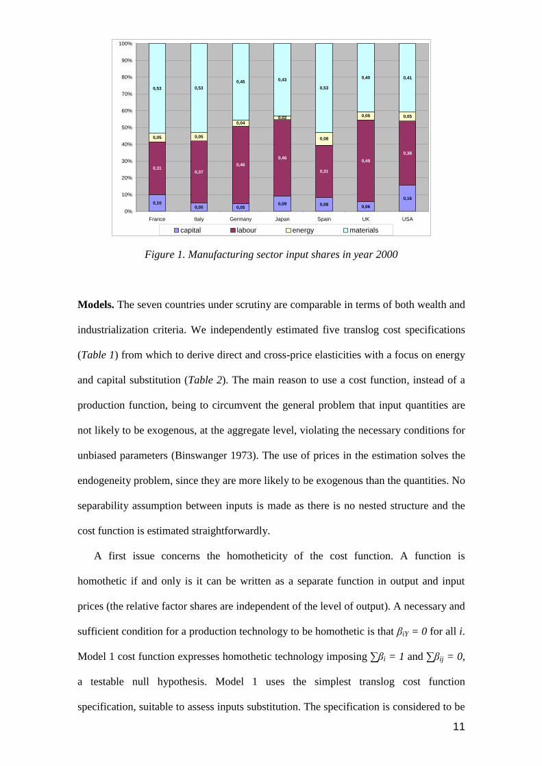
The input shares of capital, energy, labour and materials for the manufacturing

sector in the countries analysed are presented in Figure 1. The USA have the highest

capital share (16%, followed by France at 10%); the share of labour is the highest in UK

and the lowest in France and Spain, while the energy shares lie in the 4-5% range except

for Spain and Japan; materials share is between 40% in the UK and 53% in France, Italy

and Spain.

11

0,100,05 0,05

0,09 0,080,06

0,16

0,310,37

0,46

0,46

0,31

0,49

0,38

0,05 0,05

0,04

0,02

0,08

0,05 0,05

0,53 0,53

0,45 0,43

0,53

0,40 0,41

0%

10%

20%

30%

40%

50%

60%

70%

80%

90%

100%

France Italy Germany Japan Spain UK USA

capital labour energy materials

Figure 1. Manufacturing sector input shares in year 2000

Models. The seven countries under scrutiny are comparable in terms of both wealth and

industrialization criteria. We independently estimated five translog cost specifications

(Table 1) from which to derive direct and cross-price elasticities with a focus on energy

and capital substitution (Table 2). The main reason to use a cost function, instead of a

production function, being to circumvent the general problem that input quantities are

not likely to be exogenous, at the aggregate level, violating the necessary conditions for

unbiased parameters (Binswanger 1973). The use of prices in the estimation solves the

endogeneity problem, since they are more likely to be exogenous than the quantities. No

separability assumption between inputs is made as there is no nested structure and the

cost function is estimated straightforwardly.

A first issue concerns the homotheticity of the cost function. A function is

homothetic if and only is it can be written as a separate function in output and input

prices (the relative factor shares are independent of the level of output). A necessary and

sufficient condition for a production technology to be homothetic is that βiY = 0 for all i.

Model 1 cost function expresses homothetic technology imposing ∑βi = 1 and ∑βij = 0,

a testable null hypothesis. Model 1 uses the simplest translog cost function

specification, suitable to assess inputs substitution. The specification is considered to be

12

well-behaved if the first derivatives are positive and the Hessian is negative semi

definite. Since unconstrained model often verify ∑βij ≠ 0, a further direct test for

homothetic cost function is to include output as an independent variable in the estimated

equations. Model 2 includes linear, quadratic and input-specific RTS structures, to

verify the hypothesis of non-homothetic technology by including gross output of the

manufacturing sector (y) as an exogenous variable with the constraint ∑βiY = 0.11,12

Table 1. Estimated models

Model Equation Remarks

1

n

i

n

jjiij

n

iiit pppC

1 110 lnln

2

1lnln

Cost

function

2

m

ititiY

m

i

m

jjtitij

m

iititYYtYt yppppyyC

11 11

20 lnlnlnln

2

1lnln

2

1lnln

CF with

RTS

3

m

ititiT

m

i

m

jjtitij

m

iititTTtTt tppppttC

11 11

20 lnlnln

2

1ln

2

1ln

CF with

TC

4

m

i

m

jjtitij

m

iititTtYt ppptyC

1 110 lnln

2

1lnlnln

CF

constant

RTS,

neutral TC

5 m

ititiTttYT

m

ititiY

m

i

m

jjtitij

m

iititTTtTtYYtYt

tptyyppp

pttyyC

111 1

1

220

lnlnlnlnlnln2

1

ln2

1ln

2

1lnln

CF with

input

specific

RTS and

TC

Another investigation path, concerning magnitude and quality of TC, is detailed in

Model 3, where linear, quadratic and input specific TC parameters (by a time trend) are

added. In aggregate analysis ‘technology’ represents the set of possible combinations of

11

Failure to reject the null hypothesis βiY = 0 indicates homothetic production. If the coefficient βiY is

significant but all of the βij terms are not, factor shares are constant along production isoquants implying

unit own factor price elasticities. 12

Koetse (2006) noted how not including RTS parameters in the cost function systematically affects the

elasticity. In particular, if constant returns to scale do not hold in reality, primary studies that do not allow

for non-constant returns to scale will underestimate substitution potential.

13

factor inputs that can produce a given level of output. 13

Analytically, a change in

technology t shifts the isoquant structure through a change in parameter β0 in the cost

function; Model 3 and 5 include input-specific technical change parameters βiT under

the usual constraint ∑βiT = 0. The assumption of neutral technical change is generally

rejected in empirical studies (Hesse and Tarkka 1986; Hunt 1986). A diagrammatic

interpretation of energy-saving/using technical change is given in Figure 2, where the

shift to the green (red) isoquants leads to a new energy saving (resp. using) equilibrium.

Since empirical studies often assume an homogeneous cost function, with constant RTS

and neutral TC (i.e. βiy = βit = 0), we specify Model 4, with constant and neutral RTS

and TC parameters, while Model 5 gathers both flexible RTS and TC structures.

A - Substitution and neutral technical change

B - Energy-saving/using technical change

Figure 2. Substitution and technical change (adapted from Sorrell and Dimitropoulos 2007)

In our estimations we assume constant time trend t, so that a negative value of βit

implies that the share of factor i in total costs will fall over time, a positive value an

increase. The cross-price elasticity CPEij, the direct price elasticity PEii and their

variances are computed from the parameters as indicated in Table 2.

13

Binswanger (1974) proposed a definition of biased technical change suitable for functions with many

inputs, called factor price bias, giving a measure of the rate of change in the share of factor costs in the

value of output, holding input prices constant. If this factor price effect is negative, technical change is

factor-saving for factor i, if positive, is ‘factor-using’.

14

Table 2 - Elasticities and their variances

Elasticity Variance

i

ijjijij s

sCPE 2ˆ

ˆvar)var(

i

ijij s

CPE

i

iiiiiiii s

ssPE

2

2ˆ

ˆvarvar

i

iiii s

PE

4. Results

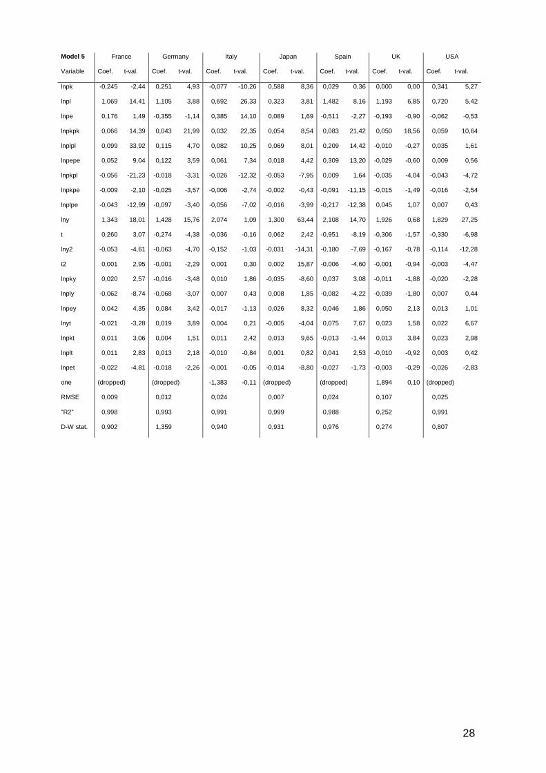
The estimated elasticities, presented in Table 3, result from the joint estimation of cost

function and input shares by three-stage iterated least squares, while cost function

estimates are presented in the Annex. The materials cost share is eliminated and the

remaining inputs prices are expressed relative to PM, to avoid redundancy. The

adequacy of the translog model is evaluated by multiple criteria: first of all negative

direct price elasticities (PEij) are expected, then we checked the (eventual pattern of)

residuals and the significance of parameters βke, βk and βe; finally, the model diagnostics

(RMSE, R2 and D-W) are used to select the best specification for each country and

relative energy/capital cross-price elasticities CPEij.

The PEij are correct for all models in France, the CPEke ranging from -0.94 to 0.04

and significant β’s over each model. The residuals pattern and regression diagnostics

lead us to retain Model 5, with a CPEke = -0.04 and CPEek = -0.06; direct elasticities are

PEk = -0.33 and PEe = -0.22. The technological structure of French manufacturing

sector indicates complementarity between K and E, significant input-specific RTS

parameters (negative for Labour) and positive input-related TC (negative for energy).

Comparison of our CPE estimates with the existing literature is hard to perform for

France: Griffin and Gregory (1976) obtain a CPEke = 0.11 (not significant) and CPEek =

0.27 (significant) with a KLEM model using panel data for 1965; estimates by Hesse

15

and Tarkka (1986) result in a CPEek = 0.023 between capital and fossil fuels in 1977,

while we considered aggregate energy as input (and France has a high nuclear share).

Both cross-price elasticities are steadily negative in Germany, while positive PEe

appear in Model 2, 3 and 5; the regression diagnostics lead us to retain Model 5 with

CPEke = -0.372 and CPEek = -0.36. Direct capital elasticity is -0.35 (PEe not

significant). German estimates by Welsch and Ochsen (2005) find CPEke = -0.13 and

CPEek = -0.32 between 1976 and 1988; the only other significant estimates for Germany

are by Falck and Koebel (1999), who obtain CPEke = 0.01 and CPEek = 0.03 (they

analyzed 27 German industries using a normalized quadratic cost function,

distinguishing between three types of labour over the 1978-1990 timeframe). Both

capital and energy direct elasticities are correctly negative for Italy; positive CPE arise

in models 1 and 3, where βke are non-significant. Based on the significance of the

parameters, residuals and diagnostics, we retain Model 5 with CPEke = -0.02 and CPEek

=-0.007; direct energy and capital price elasticities are -0.50 and -0.41, respectively.

These results can be compared with Pindyck (1979) CPEke = -0.05 and CPEek = -0.28

(in a KLE model with panel data for 1965-1973). Italian CPEke and CPEek estimates

have also been provided by Apostolakis (1990), resulting in 0.58 and 0.3 (KLE model,

evaluated in 1984, no standard error provided). Medina and Vega-Cervera (2001) find a

CPEke = -0.02 in 1988 (low significance) and, finally, Hesse and Tarkka (1986) obtain a

slightly-significant estimate of CPE between capital and fossil fuels of 0.027 in 1977.

As the direct elasticities for both energy and capital input are constantly negative for

Japan, we restrict our choice by looking at significance of the parameters βke, βk and βe.

This lead us to retain Model 4 where, accepting a lower D-W compared to Mod. 5, all

relevant β are significant. So, Japan CPEke = 0.34 and CPEek = 0.40, indicating weak

substitution between E and K; direct capital and energy price elasticity are high: -1.25

and -1.29 respectively. Norsworthy and Malmquist (1983) Japan CPEke estimates is -

0.37 for 1977 (no standard error) in a model with constant returns to scale and biased

16

technological change; estimates by Pindyck (1979) show complementarity between

energy and capital in the Japanese manufacturing sector. The five specifications result

in positive energy price elasticity in Spain, this is probably due to the lack of variations

in Spanish energy prices, making it impossible for the model to capture the mechanism

of price reaction. Negative cross-price elasticities are generally reported though,

supporting the hypothesis of a complementarity relation between energy and capital.

Lack of significance of the βk and βe parameter in, respectively, Model 5 and 3 is

compensated by the strong significance of the βke parameter, further regression

diagnostics check leaves a degree of uncertainty between Model 2 and 5, so that

Spanish CPEke might range between -0.80 and -0.83, while the CPEek is between -1.04

and -1.20 (PEk = -0.3, while PEe is not significant). The Spanish results can only be

compared with those obtained from models without material input by Apostolakis

(1987), CPEke = 0.49 in 1984, (no standard error given) and Medina and Vega-Cervera

(2001) CPEke = -0.0023 for 1988 (not significant). All five specification tested have

positive autocorrelation in the case of UK, with the D-W statistic constantly below one;

the analysis of cost function parameters significance restricts our choice to Model 2,

retaining CPEke = -0.69 and CPEek = -0.58: K/E complementarity in the UK; direct

capital and energy elasticities are -0.20 and -0.27 respectively. United Kingdom

estimates by Hunt (1986) are positive, significant and < 1 (CPEke = 0.17 in 1980, in a

model with input-specific technical change), with labour-saving and K, E-using TC. In

our estimation, both linear and quadratic returns to scale are highly significant, while

negative βlY mean labour-saving RTS. The USA estimation produces the correct price

elasticity for all specifications considered, the pseudo-R2 and D-W statistics make us

opt for model 5 to describe the manufacturing technology of the US, even though βe is

not significant, thus weakening the validity of results. Finally, USA cross-price

elasticities are CPEke = -0.08 and CPEek = -0.10. Significant energy and capital saving

TC are estimated, as well as neutral RTS and TC. In the past USA input substitution

17

have been assessed by many studies at the subsector (2 digit) level, only few treating the

aggregate manufacturing sector; between them Garofalo and Malotra (1984) and

Moghimzadeh and Kymn (1986), who distinguish between electric and non-electric

energy. The results of both refer the 1970’s and, generally, find weak substitution or

complementarity in all cases.

Koetse et al (2008) meta-analysis of the literature estimates finds CPEke for North

America and Europe around 0.38 and 0.34 respectively, which can be interpreted as

weak substitution characterizing the relation between energy and capital in the

aggregate manufacturing sector. In general, estimates of cross-price elasticities not

significantly different from zero mean that the production structure is quite rigid and

inputs cannot be easily substituted for one another. Our results show that energy and

capital are not substitutes since no CPE > 1, most countries feature CPE < 1 and the

retained CPE < 0 for six of the seven countries analyzed. This result should be carefully

interpreted, as the results do change with the estimated model. Nevertheless, the

translog KLEM specifications employed are rather straightforward and the elasticities

generally significant.

The overall poor substitution supports the hypothesis of a strong reliance of

advanced economies on (fossil fuels based) energy inputs, in contrast with mainstream

economics message, suggesting much potential for substitution away from energy and a

long and smooth energy transition toward renewable energy.

18

Table 3. Energy and capital Cross-price and direct elasticities

Model 1 Model 2 Model 3 Model 4 Model 5

CPEke CPEek PEk PEe CPEke CPEek PEk PEe CPEke CPEek PEk PEe CPEke CPEek PEk PEe CPEke CPEek PEk PEe

France 0,012 0,009 -1,08 -0,93 -0,09 -0,12 -0,45 -0,02 0,041 0,073 -0,87 -0,772 -0,94 -0,16 -0,34 -0,86 -0,04 -0,06 -0,33 -0,23

0,000 0,000 0,001 0,000 0,001 0,002 0,001 0,006 0,000 0,001 0,000 0,002 0,008 0,000 0,010 0,001 0,003 0,005 0,003 0,009

Germany -0,466 -0,214 -0,638 -0,723 -0,915 -0,896 -0,202 2,132 -0,229 -0,477 -0,648 1,781 -0,764 2,663 -0,599 -6,814 -0,372 -0,357 -0,319 0,934

0,001 0,000 0,000 0,002 0,014 0,013 0,002 0,158 0,005 0,020 0,000 0,484 0,001 0,017 0,001 0,085 0,015 0,014 0,001 0,309

Italy 0,136 -0,017 -1,444 -1,137 -0,059 -0,030 -0,425 -0,739 0,251 0,121 -0,712 -0,916 0,078 -0,011 -1,450 -1,054 -0,015 -0,007 -0,409 -0,496

0,037 0,001 0,014 0,002 0,001 0,000 0,001 0,006 0,002 0,000 0,001 0,003 0,033 0,001 0,014 0,002 0,002 0,000 0,001 0,007

Japan -0,008 -0,033 -1,090 -0,548 -0,057 -0,201 -1,077 -0,299 0,141 0,500 -0,873 -0,782 0,336 0,398 -1,246 -1,292 0,013 0,050 -0,596 -0,396

0,000 0,001 0,000 0,005 0,000 0,001 0,001 0,016 0,000 0,006 0,001 0,006 0,000 0,000 0,000 0,001 0,001 0,017 0,004 0,020

Spain -1,294 -3,259 -0,047 5,880 -0,803 -1,038 -0,298 2,579 -0,684 -9,206 -0,514 24,449 -0,829 -0,635 -0,353 0,409 -0,832 -1,205 -0,284 3,342

0,004 0,023 0,001 0,126 0,004 0,007 0,001 0,084 0,002 0,429 0,000 6,118 0,002 0,001 0,000 0,008 0,007 0,014 0,001 0,112

UK -0,509 -0,059 -0,339 -1,340 -0,693 -0,581 -0,196 -0,266 0,033 0,074 -0,712 -0,789 -0,404 -0,269 -0,739 -0,411 -0,175 -0,151 -0,258 -1,479

0,004 0,000 0,002 0,000 0,012 0,008 0,002 0,158 0,002 0,012 0,000 0,658 0,003 0,001 0,001 0,014 0,028 0,021 0,002 0,466

USA -0,362 0,885 -1,338 -1,136 -0,387 -0,635 -0,470 -0,563 -0,070 -0,156 -0,856 -0,776 -0,119 0,875 -1,573 -1,440 -0,077 -0,105 -0,544 -0,964

0,000 0,001 0,000 0,001 0,002 0,006 0,005 0,010 0,001 0,005 0,001 0,016 0,000 0,007 0,000 0,007 0,004 0,007 0,003 0,042

19

5. Conclusions

In this article, we aimed to provide an updated estimation of energy-capital substitution for

various countries. The overall purpose was to examine whether energy efficiency and

technological change have played an important role in advanced economies, thus supporting

the decoupling hypothesis, and providing input for public policy responses to increasing fossil

fuel scarcity and climate change. Our results find that a complementarity relation between

energy and capital characterizes the technology of the manufacturing sector in seven major

OECD economies for the period 1970-2005 (starting date differs between countries). This

means a strong reliance of manufacturing in all these countries on energy and mineral

resources.

In particular, strong complementarity is found for Germany, Spain and the UK, while

negative, close-to-zero crossed elasticities are estimated for France, Italy and the USA. The

weak substitution of Japan, consistent with the neutral, linear returns to scale (RTS) and

technological change (TC) specification (Model 4), comes out as statistically performing the

best. The specification with both linear and quadratic input-specific RTS and TC terms

(Model 5) turns out to best describe the manufacturing technologies of France, Germany,

Italy, Spain (Model 2 also performs well here) and the USA. An input-specific RTS

specification without TC (Model 2) best fits the UK. These differences in “best models” can

be explained by differences in the composition and technologies of manufacturing in these

various countries.

Significant capital-using TC in France, Italy and the USA and energy-saving TC in

France, Germany Japan and the USA were found. Furthermore, significant energy-using RTS

was found to apply to the UK, and significant labour-saving RTS for France, Germany and

Spain, while France and Germany also showed labour-using TC. Finally, labour-saving RTS

were found to characterize UK manufacturing, while significant neutral TC and RTS

characterize Japan. These results indicate few opportunities for decoupling between

production (GDP) and energy in Italy, Spain and the UK.

20

The world is facing a trend of increasing resource scarcity (notably peak oil) and

environmental problems (notably climate change). The solution that can count on most

support is relieving the dependence on fossil fuels by developing renewable energy. However,

increasing the share of renewable energy in total energy provision also mean less available

energy and more expensive energy, mainly because of a considerably lower energy return on

energy investment (EROI) for renewable sources compared to fossils (Murphy and Hall,

2010). Higher energy prices, given the energy-capital complementarity relation found here, in

turn imply less capital use, which is likely to result in a lower output in the manufacturing

sector.

This suggests the need for a deep restructuring of OECD economies that goes beyond an

increase in the share of renewable energy efficiency improvements. A steady policy focus on

lowering net energy consumption is needed, both on a national and per-capita basis. This will

be impossible without considerably increasing energy prices through climate-energy policies

which assures that all energy-intensive goods and services provide adequate signals to

producers, consumers and innovators alike. This will set in motion the “deep restructuring”,

which will particularly affect energy-intensive manufacturing activities like consumer

electronics, plastics, cement and glass production.

21

References

Aleklett, K., Höök, M., Jakobsson, K., Lardelli, M., Snowden, S. and Söderbergh, B. (2009):

The Peak of the Oil Age – Analyzing the world oil production Reference Scenario in

World Energy Outlook 2008, Energy Policy, Vol. 38, 1398-1414.

Apostolakis, B. E. (1987): The Role of Energy in Production Functions for Southern

European Economies. Energy, Vol. 12, No. 7:531-541.

Apostolakis, B. (1990): Energy-capital substitutability/complementarity The dichotomy,

Energy Economics, Vol. 12, 48-58.

Arrow KJ, Chenery H.B., Minhas B., Solow, R. (1961): Capital-Labour substitution and

economic efficiency, Review of Economics and Statistics, Vol. 43, 225-250.

Baldwin, J.R. and Gu, W. (2007): Multifactor Productivity in Canada: An Evaluation of

Alternative Methods of Estimating Capital Services, The Canadian Productivity Review,

no. 15-206-XIE — No. 009

Berndt, E.R. and Wood, D. O. (1975): Technology, prices, and the derived demand for

energy, The Review of Economics and Statistics, Vol. 57, No. 3 (Aug., 1975), 259-268.

Binswanger, H. (1973): A cost function approach to the measurement of elasticities of factor

demand and elasticities of substitution, University of Minnesota, Staff Paper P73-12.

Broadstock, D.C., Hunt, L.C., Sorrel, S. (2007): UK Energy Research Centre,Review of

evidence for the rebound effect, Technical Report 3: Elasticity of substitution studies.

Christensen L.R. DW Jorgenson, LJ Lau, (1971): Conjugate duality and the transcendental

logarithmic production function (Abstract), Econometrica, 1971, (p.255-256).

Christensen, L.R., Jorgenson, D.W. and Lau, J.L. (1973): Transcendental logarithmic

production frontiers, The Review of Economics and Statistics, Vol. 55, No. 1 (Feb 1973),

28-45.

Daly, H. (1997a): Georgescu-Roegen versus Solow/Stiglitz, Ecological Economics 22, 261-

266.

Daly, H. (1997b). Reply to Solow/Stiglitz, Ecological Economics 22, 271-273

22

Dasgupta, P., Heal, G. (1974): The optimal depletion of exhaustible resources, Review of

Economic Studies (Symposium), p. 3-28.

Diewert, W. Ervin, (1974): Applications of duality theory, Ch. 3 in Frontiers in Quantitative

Economics, Vol. II, ed. M.D. Intriligator and D.A. Kendrick, 1974, North-Holland.

Falk, M., Koebel, B., 1999. Curvature Conditions and Substitution Pattern among Capital,

Energy, Materials and Heterogeneous Labour. ZEW Discussion paper, vol. 99-06. ZEW,

Mannheim.

Field, B.C., and Grebenstein, C. (1980): Capital-energy substitution in U.S. manufacturing,

The Review of Economics and Statistics, Vol. 62, No. 2, 207-212.

Frondel, M. (2001): Empirical and theoretical contribution to substitution issues, PhD

dissertation.

Frondel, M., Schmidt, C.M. (2004): Facing the truth about separability nothing works without

energy, Ecological Economics 51, 217-223.

Fuss, M. and Mc Fadden, D. eds. (1978): Production economics: A dual approach to theory

and applications, North Holland.

Gagnon, N., Hall, Charles A.S., Brinker, L. (2009): A preliminary investigation of energy

return on energy investment for global oil and gas production, Energies, 2, 490-503.

Garofalo, G. A. and Malhotra, D. M. (1984): The impact of changes in input prices on net

investment in U.S. manufacturing, Atlantic Economic Journal, Vol. 13, 52-62.

Georgescu-Roegen, N. (1971), The Entropy Law and the Economic Process, Harvard

University Press.

Griffin, J., Gregory, P. (1976): An intercountry translog model of energy substitution

responses The American Economic Review, Vol. 66, No. 5 (Dec., 1976), 845-857.

Heady, E. and Dillon, J. (1962): Agricultural Production Functions, Iowa University Press

1962.

23

Hesse, D.M. and Tarkka, H. (1986): The demand for capital, labor and energy in european

manufacturing industry before and after the oil price shocks, The Scandinavian Journal of

Economics, Vol. 88, 529-546.

Hicks, John R. (1932): Theory of Wages, London, MacMillan, 1932.

Hicks, John R., Allen, R.JD. (1934): A Reconsideration of the Theory of Value, Part 2

Mathematical Theory of Individual Demand Functions, Economica, New Series, Vol. 1,

No. 2 (May, 1934), pp. 196-219.

Humphrey, T. M., Algebraic Production Functions and Their Uses Before Cobb-Douglas,

Federal Reserve Bank of Richmond Economic Quarterly Vol. 83/1 Winter 1997

Hunt, C. L. (1986): Energy and capital: substitutes or complements? A note on the importance

of testing for non-neutral technical progress, Applied Economics, 18, 729-735.

IEA (2010): World Energy Outlook 2010, Key Graphs.

Kerr, Richard (2011): Peak oil production may already be here, Science, 25 March 2011, Vol.

331.

Kallis, G., In defence of degrowth, Ecological Economics, Vol. 70, Issue 5, 873-880.

Koetse, M.J. (2006): Determinants of investment behaviour methods and applications of

meta-analysis, PhD Dissertation.

Koetse, M.J., De Groot, H.L.F., Florax, R. (2008): Capital-energy substitution and shifts in

factor demand: A meta-analysis, Energy Economics 30, 2236–2251.

Meadows, D.H., Meadows, D., Randers, J., Behrens III, William W.. (1972), The Limits to

Growth. New York: Universe Books.

Medina, J. and Vega-Cervera, J.A. (2001): Energy and the non-energy inputs substitution:

evidence for Italy, Portugal and Spain, Applied Energy 68, 203-214.

Miller, E.M. (1986): Cross-sectional and time-series biases in factor demand studies:

explaining energy-capital complementarity, Southern Economic Journal, Vol. 52, 745-

762.

24

Miller, Richard G., (2011): Future oil supply: The changing stance of the International Energy

Agency, Energy Policy, Vol. 39, 1569-1574.

Moghimzadeh, M. and Kymn, K.O. (1986): Energy-capital and energy-labor:

complementarity and substitutability, Atlantic Economic Journal Vol. 13, 44-50.

Nerlove, M. (1963): Returns to scale in electricity supply, Ch. 7 of Measurement in

Economics, pp. 167-98, C. Christ, et al, eds. Stanford University Press, 1963.

Norsworthy, J.R. and Malmquist, D.H. (1983): Input measurement and productivity growth in

japanese and U.S. manufacturing, The American Economic Review, 73, 947- 67.

Pindyck, Robert S., Interfuel Substitution and the Industrial Demand for Energy: An

International Comparison, The Review of Economics and Statistics, Vol. 61, No. 2, pp.

169-179

Robinson, J. V. (1933): The Economics of Imperfect Competition, London, Macmillan, New

York, St. Martins Press.

Salameh, M. G. (2010): An impending oil crunch by 2015?, USAEE-IAEE WP 10-054

Solow, R. M. (1987): The capital-energy complementarity debate revisited, The American

Economic Review, Vol. 77, 605-614.

Solow, R. M. (1997): Georgescu-Roegen versus Solow/Stiglitz, Ecological Economics, Vol.

22, 267-268.

Sorrell, S. (2008): Energy-capital substitution and the rebound effect, Paper for the 7th BIEE

Academic Conference.

Sorrell et al. (2010)a, Sorrell, S., Speirs, J., Bentley, R., Brandt, A., Miller, R. (2010): Global

oil depletion: A review of the evidence, Energy Policy 38 (2010) 5290–5295.

Sorrell et al. (2010)b, Sorrell, S., Miller, R., Bentley, R., Speirs, J. (2010): Oil futures: A

comparison of global supply forecasts, Energy Policy 38 (2010) 4990–5003.

Stern D. I. (2007): The elasticity of substitution, the capital-energy controversy, and

sustainability, in: J. D. Erickson and J. M. Gowdy (eds.) Frontiers in Ecological

Economic Theory and Application, Edward Elgar, Cheltenham.

25

Stiglitz, J. (1974): Growth with exhaustible natural resources efficient and optimal growth

Paths, Reviews of Economic Studies, Vol. 41, 123-137.

Stiglitz, J. (1997): Georgescu-Roegen versus Solow/Stiglitz, Ecological Economics, Vol. 22,

269-270.

Timmer, M., van Moergastel, T., Stuivenwold, E. (2007): EU-KLEMS Growth and

productivity accounts, Version 1.0, PART I Methodology.

Uzawa, Hirofumi (1962): Production functions with constant elasticities of substitution, The

Review of Economic Studies, Vol. 29,. 291-299.

van den Bergh, J. (2011) Environment versus growth — A criticism of "degrowth" and a plea

for "a-growth", Ecological Economics, Vol. 70, Issue 5, 881-890.

Welsch, H. Ochsen, C. (2005): The determinants of aggregate energy use in West Germany:

Factor substitution, technological change, and trade, Energy Economics 27, 93-111.

Wicksteed, P.H. (1894) An Essay on the Co-ordination of the Laws of Distribution,

Macmillan & Co., London.

26

Annex 1 – Model estimates

Model 1 France Germany Italy Japan Spain UK USA

Variable Coef. t-val. Coef. t-val. Coef. t-val. Coef. t-val. Coef. t-val. Coef. t-val. Coef. t-val.

lnpk 0,169 64,96 0,108 180,7 -0,027 -14,81 0,165 65,43 0,073 104,9 0,059 33,03 0,463 184,6

lnpl 0,615 153,0 0,656 142,1 0,812 492,9 0,795 274,11 0,898 294,6 0,427 62,67 0,727 289,0

lnpe 0,216 110,0 0,236 53,27 0,215 75,04 0,040 28,61 0,029 10,02 0,513 69,23 -0,190 -87,56

lnpkpk 0,014 3,62 0,051 21,47 0,013 3,98 0,012 5,42 0,075 34,09 0,043 18,49 0,058 5,81

lnplpl 0,006 0,69 0,020 2,31 0,034 9,56 0,016 5,39 0,082 11,78 0,010 1,08 -0,041 -4,85

lnpepe 0,061 12,97 0,121 12,50 0,017 1,72 0,020 7,32 0,200 19,49 0,089 8,56 0,062 8,97

lnpkpl 0,020 3,56 0,025 14,45 -0,015 -5,91 -0,004 -1,76 0,022 8,42 0,018 7,38 0,023 3,07

lnpkpe -0,034 -11,28 -0,076 -20,22 0,002 0,41 -0,008 -7,37 -0,096 -21,97 -0,061 -15,42 -0,080 -11,96

lnplpe -0,027 -5,83 -0,045 -5,34 -0,019 -3,46 -0,012 -6,04 -0,104 -13,93 -0,028 -3,06 0,018 3,24

one 12,65 3254 14,05 1422 12,36 1850,0 18,84 2064,7 12,59 659,8 13,19 540,1 14,98 1107,3

RMSE 0,350 0,455 0,421 0,192 0,418 0,560 0,314

"R2" -3,120 -8,086 -1,660 0,486 -2,674 -19,66 -0,507

D-W stat. 0,002 0,004 0,008 0,042 0,010 0,008 0,014

Model 2 France Germany Italy Japan Spain UK USA

Variable Coef. t-val. Coef. t-val. Coef. t-val. Coef. t-val. Coef. t-val. Coef. t-val. Coef. t-val.

lnpk -0,467 -15,69 -0,091 -1,97 -0,084 -14,28 0,535 4,86 0,056 2,80 -0,172 -5,81 -0,117 -2,79

lnpl 1,562 40,67 1,655 9,28 0,856 38,28 0,422 3,43 1,278 18,92 0,821 7,81 0,862 13,68

lnpe -0,095 -2,94 -0,564 -2,89 0,228 10,37 0,043 0,95 -0,334 -4,30 0,351 2,74 0,255 6,15

lnpkpk 0,053 18,95 0,048 18,70 0,030 21,15 0,003 0,83 0,085 31,72 0,054 21,36 0,078 9,15

lnplpl 0,093 19,66 0,122 7,55 0,050 7,16 0,006 1,29 0,196 12,99 0,018 0,96 0,005 0,33

lnpepe 0,065 13,86 0,184 8,03 0,034 4,81 0,021 5,76 0,297 12,60 0,060 2,03 0,037 5,11

lnpkpl -0,040 -14,54 0,007 1,43 -0,023 -14,49 0,006 1,77 0,008 1,67 -0,006 -1,18 -0,023 -2,35

lnpkpe -0,013 -4,72 -0,055 -8,28 -0,008 -4,43 -0,009 -8,05 -0,093 -13,46 -0,048 -7,08 -0,055 -10,05

lnplpe -0,052 -12,89 -0,129 -6,97 -0,027 -3,88 -0,012 -3,66 -0,204 -11,11 -0,012 -0,52 0,018 2,08

lny 1,774 123,52 1,684 32,18 0,039 0,22 1,495 90,46 -9,019 -17,29 -4,918 -8,14 -2,181 -4,34

lny2 -0,119 -54,52 -0,101 -13,25 0,004 0,33 -0,052 -30,15 0,708 18,16 0,348 7,83 0,160 4,86

lnpky 0,050 22,80 0,014 2,93 0,014 6,35 -0,017 -3,17 0,020 5,92 0,008 1,65 0,023 7,49

lnply -0,090 -32,79 -0,102 -7,68 -0,017 -3,41 -0,008 -1,35 -0,046 -6,94 -0,043 -3,01 -0,017 -4,01

lnpey 0,040 15,27 0,088 5,43 0,003 0,55 0,025 10,51 0,027 2,84 0,035 1,97 -0,007 -1,65

one (dropped) (dropped) 11,91 9,72 (dropped) 69,54 19,97 47,31 11,46 29,18 7,60

RMSE 0,010 0,029 0,040 0,030 0,041 0,115 0,100

"R2" 0,996 0,964 0,976 0,988 0,964 0,131 0,847

D-W stat. 0,815 0,570 0,296 0,474 0,318 0,321 0,074

27

Model 3 France Germany Italy Japan Spain UK USA

Variable Coef. t-val. Coef. t-val. Coef. t-val. Coef. t-val. Coef. t-val. Coef. t-val. Coef. t-val.

lnpk 0,247 175,86 0,099 193,9 0,081 51,71 0,173 77,32 0,146 171,9 0,104 59,70 0,178 139,17

lnpl 0,614 526,48 0,856 386,2 0,749 337,8 0,778 226,61 0,849 335,5 0,850 132,6 0,741 311,42

lnpe 0,139 80,25 0,045 17,50 0,170 56,23 0,049 23,86 0,005 1,53 0,046 6,10 0,080 45,39

lnpkpk 0,089 19,44 0,044 24,35 0,030 14,09 0,052 7,96 0,091 33,21 0,041 26,06 0,057 10,21

lnplpl 0,092 22,75 0,123 5,23 0,085 10,49 0,097 8,97 0,163 9,34 0,050 1,46 0,028 1,48

lnpepe 0,049 8,82 0,133 4,06 0,042 4,25 0,013 3,57 0,272 10,29 0,012 0,32 0,024 2,40

lnpkpl -0,066 -20,14 -0,017 -3,28 -0,037 -10,44 -0,068 -9,19 0,009 1,84 -0,039 -7,89 -0,031 -3,40

lnpkpe -0,022 -5,40 -0,027 -4,03 0,007 1,88 0,016 4,37 -0,100 -14,27 -0,001 -0,27 -0,026 -4,89

lnplpe -0,026 -7,27 -0,106 -3,86 -0,049 -5,85 -0,029 -5,50 -0,172 -8,16 -0,011 -0,30 0,002 0,19

t -0,013 -2,64 0,042 9,43 0,042 20,16 0,053 7,20 -0,003 -0,49 0,015 4,48 0,058 12,78

t2 0,001 3,28 0,000 1,06 0,000 -2,83 -0,001 -1,85 0,003 9,77 0,001 2,22 -0,001 -3,02

lnpkt 0,009 1,75 0,002 0,48 0,012 5,42 -0,002 -0,34 0,007 1,11 0,015 8,43 0,016 4,75

lnplt -0,014 -3,00 -0,025 -2,95 -0,023 -5,91 -0,033 -5,27 -0,035 -3,13 -0,011 -1,54 -0,004 -0,99

lnpet 0,005 0,58 0,023 2,02 0,011 2,49 0,034 3,79 0,028 1,82 -0,004 -0,54 -0,012 -2,49

one 13,16 1121,8 12,84 1023 12,56 467,1 18,63 981,0 12,08 484,9 12,2 331,2 13,55 870,77

RMSE 0,081 0,365 0,072 0,153 0,063 0,339 0,464

"R2" 0,781 -4,847 0,923 0,676 0,917 -6,555 -2,303

D-W stat. 0,042 0,015 0,119 0,052 0,190 0,020 0,012

Model 4 France Germany Italy Japan Spain UK USA

Variable Coef. t-val. Coef. t-val. Coef. t-val. Coef. t-val. Coef. t-val. Coef. t-val. Coef. t-val.

lnpk 0,033 17,06 0,099 170,0 -0,026 -13,74 0,292 92,15 0,105 156,5 0,101 47,01 0,599 207,1

lnpl 0,768 231,9 0,929 319,0 0,838 492,3 0,461 59,31 0,758 199,7 0,746 123,60 0,483 176,2

lnpe 0,199 94,63 -0,029 -10,24 0,187 64,72 0,247 45,68 0,137 37,2 0,152 22,42 -0,082 -52,3

lnpkpk 0,023 6,80 0,050 21,23 0,012 3,96 0,013 7,37 0,079 35,2 0,037 12,73 0,016 1,81

lnplpl 0,015 1,97 0,070 10,66 0,043 12,36 0,054 6,10 0,088 8,78 0,037 2,73 0,013 1,56

lnpepe 0,068 12,15 0,167 20,09 0,025 2,96 -0,011 -1,79 0,212 16,80 0,113 6,29 0,043 6,34

lnpkpl 0,015 3,41 0,023 13,42 -0,015 -6,92 -0,040 -10,76 0,022 8,66 0,020 5,30 0,007 0,90

lnpkpe -0,038 -12,66 -0,073 -19,48 0,003 0,61 0,026 8,81 -0,101 -22,47 -0,056 -11,13 -0,023 -3,32

lnplpe -0,030 -6,12 -0,093 -14,17 -0,028 -5,70 -0,015 -2,30 -0,110 -10,66 -0,057 -3,70 -0,020 -4,28

t -0,008 -4,68 -0,035 -10,97 -0,009 -6,13 -0,002 -4,19 0,053 7,11 -0,016 -5,76 0,001 0,37

lny 0,044 0,99 0,654 6,91 0,061 4,49 0,386 26,27 -0,675 -5,72 0,091 2,47 0,289 10,24

one 11,35 19,37 4,174 3,23 11,305 64,25 11,691 41,06 19,20 13,12 10,66 21,93 8,028 19,33

RMSE 1,092 0,580 0,738 0,027 1,258 0,896 2,151

"R2" -39,03 -13,80 -7,154 0,990 -32,21 -51,99 -69,864

D-W stat. 0,001 0,001 0,002 0,489 0,002 0,002 0,000

28

Model 5 France Germany Italy Japan Spain UK USA

Variable Coef. t-val. Coef. t-val. Coef. t-val. Coef. t-val. Coef. t-val. Coef. t-val. Coef. t-val.

lnpk -0,245 -2,44 0,251 4,93 -0,077 -10,26 0,588 8,36 0,029 0,36 0,000 0,00 0,341 5,27

lnpl 1,069 14,41 1,105 3,88 0,692 26,33 0,323 3,81 1,482 8,16 1,193 6,85 0,720 5,42

lnpe 0,176 1,49 -0,355 -1,14 0,385 14,10 0,089 1,69 -0,511 -2,27 -0,193 -0,90 -0,062 -0,53

lnpkpk 0,066 14,39 0,043 21,99 0,032 22,35 0,054 8,54 0,083 21,42 0,050 18,56 0,059 10,64

lnplpl 0,099 33,92 0,115 4,70 0,082 10,25 0,069 8,01 0,209 14,42 -0,010 -0,27 0,035 1,61

lnpepe 0,052 9,04 0,122 3,59 0,061 7,34 0,018 4,42 0,309 13,20 -0,029 -0,60 0,009 0,56

lnpkpl -0,056 -21,23 -0,018 -3,31 -0,026 -12,32 -0,053 -7,95 0,009 1,64 -0,035 -4,04 -0,043 -4,72

lnpkpe -0,009 -2,10 -0,025 -3,57 -0,006 -2,74 -0,002 -0,43 -0,091 -11,15 -0,015 -1,49 -0,016 -2,54

lnplpe -0,043 -12,99 -0,097 -3,40 -0,056 -7,02 -0,016 -3,99 -0,217 -12,38 0,045 1,07 0,007 0,43

lny 1,343 18,01 1,428 15,76 2,074 1,09 1,300 63,44 2,108 14,70 1,926 0,68 1,829 27,25

t 0,260 3,07 -0,274 -4,38 -0,036 -0,16 0,062 2,42 -0,951 -8,19 -0,306 -1,57 -0,330 -6,98

lny2 -0,053 -4,61 -0,063 -4,70 -0,152 -1,03 -0,031 -14,31 -0,180 -7,69 -0,167 -0,78 -0,114 -12,28

t2 0,001 2,95 -0,001 -2,29 0,001 0,30 0,002 15,87 -0,006 -4,60 -0,001 -0,94 -0,003 -4,47

lnpky 0,020 2,57 -0,016 -3,48 0,010 1,86 -0,035 -8,60 0,037 3,08 -0,011 -1,88 -0,020 -2,28

lnply -0,062 -8,74 -0,068 -3,07 0,007 0,43 0,008 1,85 -0,082 -4,22 -0,039 -1,80 0,007 0,44

lnpey 0,042 4,35 0,084 3,42 -0,017 -1,13 0,026 8,32 0,046 1,86 0,050 2,13 0,013 1,01

lnyt -0,021 -3,28 0,019 3,89 0,004 0,21 -0,005 -4,04 0,075 7,67 0,023 1,58 0,022 6,67

lnpkt 0,011 3,06 0,004 1,51 0,011 2,42 0,013 9,65 -0,013 -1,44 0,013 3,84 0,023 2,98

lnplt 0,011 2,83 0,013 2,18 -0,010 -0,84 0,001 0,82 0,041 2,53 -0,010 -0,92 0,003 0,42

lnpet -0,022 -4,81 -0,018 -2,26 -0,001 -0,05 -0,014 -8,80 -0,027 -1,73 -0,003 -0,29 -0,026 -2,83

one (dropped) (dropped) -1,383 -0,11 (dropped) (dropped) 1,894 0,10 (dropped)

RMSE 0,009 0,012 0,024 0,007 0,024 0,107 0,025

"R2" 0,998 0,993 0,991 0,999 0,988 0,252 0,991

D-W stat. 0,902 1,359 0,940 0,931 0,976 0,274 0,807

29

Annex 2 – EU-KLEMS Input prices

Capital price

Labour price

Energy price

Materials price

30

Annex 3 – EU-KLEMS Input shares

France Germany Italy Japan Spain UK USA sk sl Se sm sk sl se sm sk sl se sm sk sl se sm sk sl se sm Sk sl se sm sk sl se sm

1970 0,046 0,437 0,092 0,425 0,065 0,488 0,031 0,416 0,102 0,403 0,076 0,418

1971 0,039 0,462 0,088 0,411 0,062 0,456 0,071 0,411 0,114 0,397 0,076 0,413

1972 0,037 0,459 0,090 0,413 0,067 0,456 0,067 0,410 0,113 0,392 0,074 0,420

1973 0,043 0,446 0,095 0,417 0,103 0,366 0,029 0,502 0,064 0,429 0,090 0,417 0,105 0,391 0,074 0,430

1974 0,047 0,425 0,096 0,432 0,089 0,373 0,023 0,515 0,047 0,423 0,115 0,414 0,101 0,377 0,075 0,448

1975 0,030 0,452 0,099 0,418 0,089 0,401 0,020 0,490 0,041 0,444 0,099 0,415 0,120 0,372 0,080 0,428

1976 0,042 0,441 0,097 0,419 0,094 0,393 0,012 0,501 0,043 0,431 0,124 0,402 0,115 0,378 0,078 0,429

1977 0,041 0,444 0,090 0,424 0,092 0,394 0,022 0,492 0,056 0,415 0,104 0,424 0,122 0,374 0,075 0,429

1978 0,058 0,473 0,056 0,414 0,040 0,440 0,090 0,430 0,100 0,398 0,023 0,479 0,059 0,417 0,118 0,406 0,115 0,382 0,072 0,430

1979 0,053 0,472 0,056 0,419 0,042 0,429 0,091 0,438 0,096 0,381 0,022 0,501 0,054 0,465 0,064 0,417 0,109 0,388 0,077 0,427

1980 0,046 0,471 0,063 0,420 0,050 0,422 0,076 0,453 0,075 0,388 0,019 0,517 0,101 0,292 0,085 0,523 0,047 0,475 0,069 0,409 0,102 0,389 0,089 0,420

1981 0,084 0,352 0,061 0,503 0,043 0,469 0,069 0,419 0,048 0,423 0,075 0,453 0,077 0,403 0,018 0,502 0,097 0,286 0,079 0,537 0,042 0,497 0,052 0,408 0,108 0,396 0,080 0,416

1982 0,081 0,357 0,051 0,510 0,047 0,466 0,071 0,416 0,047 0,427 0,072 0,454 0,079 0,414 0,016 0,490 0,097 0,278 0,086 0,539 0,050 0,487 0,045 0,418 0,109 0,397 0,081 0,413

1983 0,086 0,358 0,048 0,509 0,052 0,464 0,067 0,417 0,044 0,436 0,067 0,453 0,077 0,425 0,017 0,481 0,102 0,270 0,075 0,554 0,059 0,480 0,059 0,403 0,113 0,387 0,071 0,429

1984 0,084 0,353 0,048 0,515 0,052 0,456 0,069 0,423 0,048 0,416 0,065 0,471 0,081 0,421 0,017 0,481 0,105 0,253 0,084 0,558 0,057 0,484 0,050 0,409 0,121 0,388 0,072 0,419

1985 0,093 0,349 0,047 0,512 0,056 0,455 0,066 0,422 0,048 0,417 0,060 0,474 0,084 0,427 0,016 0,473 0,110 0,247 0,077 0,566 0,063 0,475 0,053 0,408 0,120 0,404 0,067 0,409

1986 0,101 0,351 0,044 0,505 0,062 0,472 0,053 0,412 0,052 0,427 0,060 0,461 0,088 0,454 0,017 0,442 0,127 0,262 0,058 0,553 0,069 0,489 0,066 0,377 0,122 0,419 0,057 0,403

1987 0,096 0,356 0,043 0,505 0,055 0,480 0,063 0,402 0,052 0,429 0,052 0,466 0,090 0,465 0,017 0,428 0,123 0,270 0,058 0,549 0,067 0,506 0,049 0,379 0,129 0,402 0,060 0,409

1988 0,102 0,343 0,042 0,513 0,059 0,475 0,061 0,405 0,051 0,419 0,050 0,480 0,093 0,456 0,018 0,433 0,125 0,267 0,050 0,558 0,073 0,495 0,052 0,380 0,136 0,390 0,060 0,414

1989 0,102 0,337 0,041 0,520 0,060 0,466 0,063 0,412 0,050 0,416 0,052 0,482 0,092 0,447 0,019 0,442 0,124 0,268 0,054 0,553 0,068 0,511 0,047 0,373 0,138 0,396 0,060 0,405

1990 0,099 0,347 0,042 0,512 0,058 0,475 0,060 0,407 0,044 0,433 0,051 0,473 0,092 0,426 0,021 0,461 0,109 0,294 0,055 0,542 0,074 0,513 0,046 0,367 0,139 0,395 0,065 0,400

1991 0,097 0,353 0,044 0,506 0,055 0,484 0,056 0,405 0,040 0,461 0,050 0,449 0,093 0,430 0,022 0,455 0,104 0,307 0,053 0,537 0,060 0,514 0,045 0,380 0,140 0,398 0,062 0,399

1992 0,093 0,362 0,043 0,502 0,048 0,503 0,045 0,403 0,039 0,443 0,052 0,467 0,093 0,448 0,021 0,438 0,089 0,334 0,052 0,525 0,063 0,488 0,043 0,406 0,136 0,402 0,058 0,405

1993 0,084 0,376 0,045 0,495 0,042 0,521 0,046 0,391 0,041 0,441 0,054 0,465 0,089 0,463 0,022 0,426 0,078 0,352 0,052 0,519 0,066 0,476 0,044 0,414 0,136 0,402 0,055 0,408

1994 0,085 0,365 0,046 0,504 0,046 0,511 0,044 0,399 0,044 0,415 0,053 0,488 0,085 0,471 0,023 0,421 0,082 0,324 0,052 0,541 0,074 0,462 0,044 0,421 0,145 0,393 0,052 0,410

1995 0,092 0,352 0,046 0,510 0,043 0,499 0,047 0,411 0,046 0,384 0,052 0,517 0,087 0,465 0,023 0,425 0,097 0,322 0,057 0,524 0,076 0,449 0,045 0,430 0,148 0,378 0,052 0,422

1996 0,087 0,359 0,048 0,506 0,044 0,505 0,042 0,409 0,047 0,400 0,051 0,502 0,090 0,461 0,024 0,425 0,095 0,325 0,059 0,521 0,081 0,440 0,053 0,426 0,156 0,377 0,051 0,416

1997 0,093 0,348 0,048 0,511 0,049 0,490 0,040 0,421 0,046 0,396 0,051 0,506 0,087 0,457 0,024 0,432 0,093 0,328 0,059 0,520 0,083 0,444 0,050 0,423 0,161 0,381 0,045 0,413

1998 0,100 0,332 0,053 0,515 0,051 0,482 0,041 0,426 0,050 0,385 0,051 0,515 0,088 0,467 0,024 0,421 0,090 0,329 0,052 0,529 0,072 0,475 0,045 0,409 0,157 0,387 0,044 0,411

1999 0,097 0,328 0,053 0,521 0,050 0,482 0,036 0,431 0,048 0,386 0,049 0,518 0,089 0,473 0,023 0,415 0,087 0,328 0,058 0,527 0,067 0,485 0,045 0,403 0,162 0,385 0,045 0,408

2000 0,101 0,315 0,051 0,534 0,048 0,460 0,037 0,454 0,050 0,370 0,051 0,529 0,092 0,455 0,024 0,429 0,084 0,312 0,077 0,527 0,057 0,488 0,050 0,405 0,155 0,384 0,054 0,406

2001 0,095 0,315 0,050 0,539 0,048 0,460 0,034 0,458 0,050 0,371 0,052 0,527 0,083 0,463 0,024 0,430 0,084 0,312 0,074 0,530 0,059 0,490 0,044 0,407 0,165 0,394 0,046 0,395

2002 0,092 0,326 0,048 0,534 0,049 0,467 0,041 0,443 0,048 0,375 0,050 0,527 0,086 0,463 0,025 0,426 0,087 0,317 0,072 0,524 0,054 0,499 0,046 0,401 0,167 0,397 0,047 0,389

2003 0,088 0,337 0,047 0,527 0,052 0,462 0,044 0,442 0,043 0,383 0,051 0,523 0,093 0,448 0,024 0,435 0,088 0,318 0,074 0,520 0,050 0,500 0,048 0,402 0,167 0,403 0,044 0,387

2004 0,085 0,332 0,049 0,534 0,056 0,443 0,038 0,463 0,043 0,379 0,052 0,526 0,096 0,431 0,024 0,449 0,082 0,308 0,083 0,527 0,051 0,493 0,053 0,403 0,176 0,384 0,045 0,395

2005 0,088 0,320 0,048 0,545 0,058 0,426 0,037 0,479 0,040 0,376 0,056 0,528 0,093 0,415 0,024 0,467 0,081 0,304 0,096 0,519 0,052 0,495 0,054 0,400 0,185 0,378 0,046 0,391

Mean 0,092 0,345 0,047 0,515 0,052 0,475 0,052 0,422 0,045 0,418 0,066 0,470 0,089 0,432 0,021 0,458 0,098 0,300 0,067 0,535 0,061 0,473 0,061 0,405 0,134 0,391 0,063 0,413