Capacity Investment and Product Line Decisions of a ...646 Capacity Investment and Product Line...

Decision SciencesVolume 44 Number 4August 2013

© 2013 The AuthorsDecision Sciences Journal © 2013 Decision Sciences Institute

Capacity Investment and Product LineDecisions of a Multiproduct Leader anda Focus Strategy Entrant*H. Muge Yayla-KulluLally School of Management, RPI, Troy, NY 12180, e-mail: [email protected]

ABSTRACT

In this article, I investigate the capacity investment cost conditions where a multiproductmarket leader may respond to a focus strategy entrant by using different strategies suchas changing the product mix, production volumes, quality levels, and/or by investingin more capacity. The products offered in the market are quality differentiated and cus-tomers are heterogeneous in their willingness to pay for quality. The capacity investmentcosts of the two firms (i.e., the leader and the entrant) may also be different. The classicalStackelberg model predicts that an incumbent does not change its position in responseto entry. However, when heterogeneous customer base, product differentiation, and ca-pacity costs are taken into consideration, I find that the leader with a low capacity costmay choose to expand its product line and increase its production. The leader with lowcapacity cost may introduce a product that it was holding back when the entrant has tobear the high-capacity cost and cannibalization threat is relatively small. Nevertheless,the extent of production volume strategies reduces as the capacity cost increases for theleader. I also find that when the leader has the power to set the industry standards bydeciding the quality levels, as a response to a high-quality focused entrant, the leaderincreases both levels of quality and production of the low-quality product. Moreover,when the capacity investment cost is high for both the entrant and the leader, I find thatmarket prices may increase with entry. [Submitted: July 19, 2012. Revised: October 3,2012. Accepted: December 12, 2012.]

Subject Areas: Capacity Investment, Competition, Focus Strategy, OM-Marketing Interface, and Product Line.

INTRODUCTION

There are numerous empirical studies that show how market leaders attack newentrants in a variety of ways (Smiley, 1988; Geroski, 1991; Oster & Strong,2001). Smiley (1988) shows that 26% of the established firms choose to respondby increasing their product variety. Geroski (1995) reports some case studieswhere the incumbents introduce new products which they had been holding back.Use of capacity is another common response to the potential threat of entry. For

*The author is grateful to Prof. Jayashankar M. Swaminathan for his helpful comments on an earlierversion of this article.

645

646 Capacity Investment and Product Line Decisions

example, in the airline industry, the launch of low-cost subsidiaries like UnitedShuttle and Delta Express (new product introduction) is recorded to be a “defensiveresponse carefully targeted to the threat of Southwest and other low-cost, low-fareairlines” in a DOT report (Oster & Strong, 2001, p. 16). This report also providesspecific examples, such as Northwest’s actions toward Reno Air’s entry in Reno–Minneapolis market in 1993. Northwest not only launched a new nonstop service(increasing quality), it has also started offering additional nonstop flights fromReno to markets served by Reno Air (new product introduction). Another exampleinvolves competition in the Detroit–Philadelphia market. Spirit Airlines enteredthis market at the end of 1995 with high capacity at the low fare range. When SpiritAirlines announced its entry in other markets served by Northwest, Northwestresponded by increasing its low fare seat capacity to over 35 times more thanbefore (use of capacity) in these markets (Oster & Strong, 2001).

Major airlines have responded similarly to focus strategy competition atthe high-end market. For example, in 2007–2008, American Airlines (AA) hadincreased its service frequency and award miles program (use of capacity andincreasing quality) in the London–New York route with lower prices until thebankruptcy of the new all-business carrier, EOS. These actions toward EOS arerecorded to be predatory in the press (Rowell, 2009).

Market leaders often have a first mover advantage (Lee & Ng, 2007). Theyhave higher market shares and a better business performance. They have enoughtechnological capability and support facilities to produce multiple products orwithhold one if necessary. An entrant firm is motivated to steal business in such amarket dominated by a leader. If the leader chooses to change its product mix inresponse to the entrant, then it has to watch out for cannibalization among its ownproducts. Moreover, these changes may require additional resources. Hence, thereare intricate relationships in this game which make it difficult to predict the optimaldecision a priori. However, the existing analytical literature, by and large, overlookthe impact of such policies involving capacity and product line policies. Yet in avertically differentiated industry with multiple products (potentially consumingdifferent amounts of resources per unit), a market leader may benefit from betterutilization of costly resources under some operational conditions. In this article, Istudy such a competition between a market pioneer and a focus strategy entrantand identify such conditions analytically.

In particular, I address the following research questions: What are the opera-tional conditions that trigger a strategy change for the firms? How are the productmix and supply in the market affected by an asymmetric competition? How arecapacity investment decisions affected by the cost of such investments in a verti-cally differentiated market? What are the implications on the quality levels of theproducts?

In this stylized model, a sequential entry (Stackelberg) game between amultiproduct market leader and a focus strategy follower is studied. The leaderhas the capability to produce two vertically differentiated products with differentqualities, unit production costs, and unit resource consumptions. It moves firstand chooses which product(s) to offer, their quality levels, and how much to offerin the market. Sequentially, the entrant that has a focus (on either high or lowquality) product observes the leader’s decisions and determines its own production

Yayla-Kullu 647

quantity and necessary capacity investments. Among others the major findings areas follows:

• It is shown that the leader would be better off by expanding the productline to include the entrant’s focus product when the capacity cost is high for theentrant. The entrant generates an interest in the market for its focus product, butthe increasing capacity cost puts operational pressure on the entrant to lower theproduction. This creates an incentive for the leader (with a lower capacity cost)to proliferate and introduce this particular product, which it would hold back as amonopolist.

• Common wisdom suggests that the capacity investments should decrease asthe relevant costs increase. In contrast, I find that the entrant’s capacity investmentmay be increasing as the cost of capacity increases. When the leader offers onlythe high-quality product and the high-quality product requires lots of resources forproduction, the low-quality focused entrant is better off by increasing the supplywhich requires increasing the capacity investment.

• I also find that as a response to a high-quality focused entrant, the leaderchooses to increase both levels of quality and the production of the low-qualityproduct. It may even increase the production of the high-quality product depend-ing on its capacity investment cost. Moreover, contrary to intuition, I find thatmarket prices may increase with entry despite the competition, when the capacityinvestment cost is high for both the entrant and the leader.

The rest of the article is organized as follows. The literature review is pre-sented in the next section followed by model assumptions. Next, the problem issolved focusing on the product variety implications. Then, the implications onquality decisions are analyzed. Finally, I discuss managerial insights and concludethe article.

RELATED LITERATURE

Firms’ Reactions to Entry

There is a vast literature in marketing and economics on firms’ reactions to entry.Geroski (1995) provides a summary of the stylized facts and empirical generaliza-tions on the subject. Empirical findings suggest that increasing product variety is acommon strategy in response to entry for companies (Smiley, 1988; Neven, 1989;Geroski, 1995). In a recent paper, Dunn (2008) investigates the airline industry.He provides evidence that a firm is more likely to start a high-quality service inresponse to entry if the firm has an existing low-quality service in the market. Theauthor finds that cannibalization effects are more likely to diminish when there is“the threat of business stealing” in the market. However, analytical investigationis nonexistent in this domain especially when the products are differentiated. Inthis article, I fill this gap and analytically study the product variety changes in theface of sequential entry. I explain when a firm should proliferate as a response tocompetition when there are quality and resource consumption differences amongthe products.

There are a number of analytical papers in the entry literature that look at thecapacity investment as an entry-deterring strategy of an incumbent firm (Spence,


1977; Dixit, 1980). However, these papers have largely ignored the product varietyand resource utilization aspects of the problem. The majority of these papers focuson homogeneous products and fixed costs of capacity. The common finding is thatthe incumbent firm may invest in capacity to deter entry; and this investment mayresult in idle capacity. However, there are conflicting empirical findings on thisclaim. There are a number of studies which reject this hypothesis (Geroski, 1995).On the other hand, Conlin and Kadiyali (2006) find evidence that firms with largermarket shares (market leaders) have more (entry deterring) idle capacity than firmswith smaller market shares (followers).

I contribute to this line of literature by considering a differentiated productline that leads to additional trade-offs such as cannibalization; and by introducingpotential differences in resource consumptions of products. I show that qualitydifferentiation and resource utilization issues provide a better explanation to howfirms may or may not use capacity investments and production volume changesin response to entry. In particular, when the products consume different amountsof the costly resource, the interplay between the products for resources and thecompetitive interaction between the firms for better market share in a verticallydifferentiated industry leads to different outcomes than before.

Vertically Differentiated Product Lines

There is also a rich literature on the firm’s choice of vertically differentiatedproduct lines (Mussa & Rosen, 1978; Moorthy, 1984; Johnson & Myatt, 2003).In these studies, the major finding is that a monopolist needs to either increasethe differentiation between the products or delete the low-quality product from theproduct line in order to mitigate the effects of cannibalization. Surprisingly, thenumber of papers that study product variety choices in the case of sequential entryis quite low. This article contributes to the literature by analyzing the impact ofasymmetric competition on the decisions of the capacity-constrained multiproductfirms.

Tsikriktsis (2007) empirically studies the effects of focus strategy, capacityutilization, and conformance quality on profits of the airline industry. He showsthat the quality defects have a greater impact on the profitability of focus strategyairlines than the full-service carriers. Intuitively, focus strategy firms are moresensitive to downward changes in their operational parameters in general. Onepossible explanation I offer to his findings is the fact that the diverse firms canadapt to these changes (such as the fuel cost increase) by modifying their productlines, maybe even shifting operations from one product to another. However, focusstrategy firms have to survive with their focus product alone. Based on my studyin this article, I believe that the parametric changes in the industry could leave afocus strategy firm to operate under suboptimal conditions and lose more moneythan their diversified rivals.

Boyaci and Ray (2003) and Chayet, Kouvelis, and Yu (2009) consider ca-pacity management issues for offering differentiated product lines. They formulatethe problem as queuing models and focus on the capacity investment decisionsof monopolists in congested systems. Chayet et al. (2009) show that increasingcongestion costs results in less variety in the product line. This article shows that

Yayla-Kullu 649

Table 1: Comparison of this paper with the literature.

Method Vertical Competition CapacityDifferentiation Investment

Mussa and Rosen (1978) Analytical Yes No NoDixit (1980) Analytical No Yes YesSmiley (1988) Empirical Yes Yes YesJohnson and Myatt (2003) Analytical Yes Yes NoConlin and Kadiyali (2006) Empirical No Yes YesDunn (2008) Empirical Yes Yes NoChayet et al. (2009) Analytical Yes No YesYayla-Kullu et al. (2011) Analytical Yes No YesHaruvy et al. (2013) Analytical Yes Yes No

This article Analytical Yes Yes Yes

this may not be true when the resource consumptions of the products differ. Inaddition, the impact of competition on these decisions is discussed here.

Notably, Johnson and Myatt (2003) provide an analysis of the multiproductquality competition in duopoly and oligopoly markets, but they ignore the capacityconstraints of the firms. They aim to explain why the firms adjust their productlines (by introducing fighting brands or reducing the variety) in response to com-petition. The authors study symmetric firms as well as the competition between amultiproduct firm and a low-quality firm. They show that in the asymmetric com-petition, the incumbent continues to act like a monopolist for quality levels thatare greater than the entrant’s highest quality. In contrast, I show that all products’supplies may be affected due to the costly resource decisions of the firms. More-over, Johnson and Myatt (2003) do not consider a high-quality entrant while I do,in addition to the capacity investment decisions. Hence, this is the first article thatconsiders both high- and low-quality entry in a comprehensive model includingcapacity constraints.

More recently, Haruvy, Miao, and Stecke (2013) numerically study a sequen-tial entry game with two periods. The leader chooses a single product in the firstperiod and has the potential to offer a second differentiated product in the secondperiod in response to the entrant. They focus on identifying quality and innova-tion strategies for the incumbent while my focus is on the capacity investmentsand production quantity decisions. They ignore the capacity dimension altogetherwhich is the key parameter in this article.

In short, I contribute by considering costly capacity choices and potentialasymmetry in the product line strategy of competing firms. A tabulated summarycomparison of this article with the literature is given in Table 1. I take the costsof different actions into account in order to understand the consequences of theseactions better. For example, if the leader changes its product mix, then it has towatch out for cannibalization among its own products. Moreover, an increase inproduction may increase the resource consumptions of the products which meansmore capacity is necessary. At that point the firm needs to consider the unit


production costs and the capacity investment costs as much as the competitiveforces. Hence, introducing all these operational costs and the competitive trade-offs is a necessary contribution to the literature and I aim to fill this gap with thisarticle.

MODEL

In this stylized model, there are two products, a high (H )- and a low (L)-qualityproduct. Each unit of product i = H, L has quality qi . As the first mover, the leaderhas the power to choose these quality levels and set the standards in the market. Theleader chooses from a technologically feasible range of qualities: qi ∈ [q, q]. It isshown in the empirical literature that the new entrants have no power in shaping theindustry structure and they often start as followers of the standards set by the marketpioneers (Geroski, 1995) (unless the entrant is an innovator, which is not the focusof this article). In the airline example, this would correspond to an airline choosingfrom a number of available cabins such as economy, premium economy, business,and first class cabins. Although the type of service customers will receive withineach cabin is pretty much set by the industry standards, minor changes might bemade in terms of the service quality. For example, in a transatlantic flight, customersexpect and accept to be uncomfortable in an economy class seat, whereas industrystandards dictate that a first class customer gets gourmet food on board (Source:Skytrax Web site: airlinequality.com).

Following the literature, I assume that customers will only buy a positivequality (q > 0) or choose not to buy anything (Moorthy, 1984). Unit productioncost is ci = c(qi). It is an increasing function of quality (cH ≥ cL), and it is linear inquantity (Mussa & Rosen, 1978; Moorthy, 1984). Products may also have differentresource consumptions. Each unit of product i requires si = s(qi) units of capacity.Indeed, for the airline example, business class seats are perceived as better quality(qH > qL); they are bigger in size (sH > sL); and it costs more to serve them(cH > cL) due to the greater number of flight attendants, food and drinks, and soforth. Yayla-Kullu and Tansitpong (2011) also provide empirical support that theresource consumption differences between the products have a significant impacton airlines’ capacity allocation decisions.

I adopt the classical vertical differentiation demand model (Mussa & Rosen,1978; Moorthy, 1984; Tirole, 1988). Customers vary in their willingness to pay forquality. Following the literature, I assume that the customer types (θ) are uniformlydistributed in the unit interval [0,1] with unit total mass (cf. Tirole, 1988, p. 296). Itis necessary to assume a uniform demand distribution to make the analysis tractable.This enables us to keep the focus on the effects of capacity costs on product linechoice and to derive insights. Note also that this is a common assumption in theliterature when analysis with more general distributions is intractable (cf. Johnson& Myatt, 2006, p. 594).

When a type θ customer buys product i at price pi , her utility is equal toU (qi, pi, θ) = θqi − pi. By checking the conditions for the marginal customers,demands for the two products can be found. One such marginal customer is indif-ferent between buying a high- or low-quality product; the other one is indifferentbetween buying the low-quality product or nothing at all. Then, demands for the

Yayla-Kullu 651

two product types are as follows:

DH (pL, pH ) = 1 − pH − pL

qH − qL

, DL(pL, pH ) = pH − pL

qH − qL

− pL

qL

. (1)

Segmentation, product proliferation, and cannibalization are well-knownconflicting forces for a firm in such a quality-differentiated demand model (Mussa& Rosen, 1978; Moorthy, 1984; Tirole, 1988). In a model that does not take thecapacity constraint and competitive interactions into account, if a firm offers asingle product of high quality (product h), the total sales would be (1 − ph

qh). In-

troducing a second product of lower quality (product l) may increase the totalsales by (ph

qh− pl

ql), which would be the benefit of proliferation. Moreover, through

price discrimination, the firm further benefits from offering multiple products inthe market. However, under the same conditions, some customers switch frombuying the high-quality product to buying the low-quality product, reducing thehigh-quality sales by (ph−pl

qh−ql− ph

qh), which is known as cannibalization. In the ex-

isting literature, product line choice centers on deciding the quality differentiationin the product line, where firms analyze the trade-offs associated with the benefitsof product proliferation and the effects of cannibalization that arise from the intro-duction of a new product. Analysis of such models in terms of competition, cost,and market conditions provides insights into whether firms should offer a high- ora low-quality product (Yayla-Kullu, Parlakturk, & Swaminathan, 2011, 2013).

Suppose a full-service carrier (e.g., British Airways) has to make choices forits high-end segment in a market (e.g., Las Vegas–London route). It has the optionof offering both first and business class cabins, or it can choose to offer only one orthe other on board. If both classes are available (proliferation), a greater customerbody could be served. However, some first class cabin customers might switchto business class due to lower prices (cannibalization). The problem gets moreinteresting when an all-business class carrier (e.g., MaxJet) enters such a market,especially at a time when the fuel prices are rising and rapidly constraining thecapacity in the air.

In this stylized model there are two firms, X and Y . Firm X has the ability tomove first and assume a leader position. It can serve a subset of the two products{H, L}. It needs to decide for the quality levels of the products (qH , qL ∈ [q, q]),how much of each product (xH , xL ≥ 0) to offer in the market, and the requiredcapacity (KX) necessary to produce this quantity. On the other hand, entrant Y isa new, focus strategy firm. It has a fixed product line and produces one product.Entrant Y observes the decisions of the leader X, and sequentially determines howmuch of its product (yj ≥ 0, where j is either H or L) to offer in the marketand the required capacity (KY ) necessary to produce this quantity. Note that thecustomers are indifferent buying from either firm. In the end, prices are set to clearthe market based on the total amount of production in the industry: pH (xH , xL, yj )and pL(xH , xL, yj ).

It is assumed that the entrant has to pay γy to purchase a unit of capacity andcapacity purchase is not lumpy. On the other hand, as the pioneer in the market,the leader has a distinct cost advantage (Geroski, 1995; Lee & Ng, 2007). It hasto pay only γx where 0 ≤ γx ≤ γy to purchase a unit of capacity. This assumptionalso fits well with the airline industry, where the aircraft operational costs are


extensive. An airline should pay for aircraft leasing, fuel, and labor costs beforeallocating the aircraft space among different cabin and seat types. Aircrafts areexpensive. Airlines typically use one, or a combination, of the following tech-niques to pay for their fleet: Cash, operating leasing and sale/leasebacks, bankloans/finance leases, export credit guaranteed loans, tax leases, and manufacturersupport (source: http://www.airfinancejournal.com/). Note that, only very few well-established firms can afford to pay by cash. All of the other financing options arepriced based on the risk of the buyer airline. As mentioned earlier, it is commonknowledge that a new entrant firm is a much riskier option than an establishedmarket leader (Geroski, 1995; Lee & Ng, 2007). Hence, one would expect that anestablished airline should be able to receive better financing options compared toa new entrant airline.

In short, the decision time line is as follows: (i) The entrant announcesentry in the market. Its focus product, either H or L, is common knowledge. (ii)The leader makes necessary capacity investments and announces its product line,quality levels, and production quantities. A leader can offer any combination of thetwo products. (iii) The entrant observes the leader’s decisions, makes necessarycapacity investments, and announces its production quantity. (iv) Customers self-select from the menu of offerings and market clearing prices are observed by allagents.

This time line is consistent with many industries including the airline industry.Starting scheduled flights from one airport to another necessitates a great deal ofpaperwork and entry is public information long before any quantity decisionsare made. Note also that a focus strategy firm such as Southwest has a fixedfocus product and does not change this decision before they enter a given marketidentified by routes in the airline industry. However, I note that a full-servicecarrier such as Delta may or may not have a business class on board in additionto economy class in every route. Moreover, there are clear distinctions betweenmarket leaders and followers in every market. Many markets (identified by origin-destination pairs) have a dominant airline, mostly due to well-known hub-and-spoke systems. Hence, Stackelberg-type competition is prevalent in such marketswhere the dominant airline is the market leader and others are followers.

IMPLICATIONS ON PRODUCT VARIETY

In this section, solutions of the game for various market settings are presented andthe conditions that trigger changes in product mix, supply, and capacity investmentdecisions are discussed. I first study a monopolist’s problem and establish the basisfor comparisons. Then, two Stackelberg games that may have different outcomesdue to the leader’s capacity investment cost are analyzed.

The quality levels are fixed to two variants; this enables us to direct ourattention to the research questions about the product variety choices. There arenumerous studies in the literature that model the product line problem with nexogenous levels of quality (Bhargava & Choudhary, 2001; Johnson & Myatt, 2003;Jing, 2006). This is essentially equivalent to having a continuous range of qualities,as n could be an arbitrarily large number. The major finding is that the firm wouldoffer a full product line if the cost to quality ratio is increasing (cH/qH > cL/qL),

Yayla-Kullu 653

and only the highest quality product otherwise (cH/qH ≤ cL/qL). Having n > 2products does not change this product variety choice (Bhargava & Choudhary,2001; Johnson & Myatt, 2003). In another study, I have also shown that the sameinsights can be achieved with two exogenous quality levels as when there are n ≥ 3levels of quality (Yayla-Kullu et al., 2013). Hence, I will discuss how my findingswith asymmetric competition and resource considerations are different than sucha product line choice without loss of generality.

Note also that in the airline industry, product types (identified by differentclass cabins) are notably similar across different firms. Industry standards are setvery clearly. For example, economy seats offered by American, Delta, and Unitedin their Boeing 757–200 aircraft all have a pitch of 31 inches and a width of 17–17.2 inches. Similarly, first class seats on this aircraft have a pitch of 38–39 inchesand a width of 20.5–21 inches. Likewise, economy seats of these three airlines ontheir Canadair CRJ-700 aircraft also have pitch of 31 inches and width of 17–17.5inches (source: seatguru.com). Indeed, there are ranking firms such as Skytrax(airlinequality.com) that evaluate each airline based on these clearly set industrystandards.

In this stylized model, as the market leader, firm X expects the entrant tobehave optimally and makes decisions taking her response into account. Hence,the leader solves the following problem:

Max(KX≥0,xL≥0,xH ≥0)

(pH (xH , xL, y∗j (xH , xL)) − cH )xH

+ (pL(xH , xL, y∗j (xH , xL)) − cL)xL − γxKX, (2)

subject to sHxH + sLxL ≤ KX.

Observing the optimal decisions of the leader, entrant Y with a focus productj solves the following problem:

Max(KY ≥0,yj ≥0)

(pj (x∗H , x∗

L, yj ) − cj )yj − γyKY , (3)

subject to sjyj ≤ KY .Threshold capacity cost levels γ that may be functions of product types are

explicitly stated in Appendix A. These thresholds are useful for describing howfirms’ strategies change. All proofs appear in Appendix B.

Lemma 1: Since the objective functions given in problems (2) and (3) are jointlyconcave in their corresponding decision variables on convex solution sets definedby linear constraints, subgame perfect Nash equilibrium can be obtained by solvingthe first-order conditions and backward induction.

The lemma shows that the general form of the problem with asymmetriccosts is easily solvable. In the following subsections, I characterize the subgameperfect Nash equilibrium in closed form when the capacity cost for the leader isin the two ends of the spectrum: either zero or equal to the entrant’s cost. Then, Icomplement these results with numerical examples to show how they generalizeto a wider range of parameters. Keeping the capacity cost parameters with twovariants makes my analysis tractable allowing me to focus on the key researchquestion, and characterize the impact of asymmetric competition on firms productline choices when resources are costly. Note again that following each result, I will


present numerical examples to show how these results continue to hold in a widerrange of parameters, and how these are contradicting to the existing literature.

A Monopolist’s Product Line and Capacity Investments

A monopolist that needs to make product line decisions (xML ≥ 0, xM

H ≥ 0) andcapacity investments (KM ≥ 0) has to solve the following problem:

Max(KM≥0,xM

L ≥0,xMH ≥0)

(pH (xMH , xM

L ) − cH )xMH + (pL(xM

H , xML ) − cL)xM

L − γxKM,

(4)subject to sHxM

H + sLxML ≤ KM .

Following Lemma 1, the optimal solution can be obtained by solving the first-order conditions. Next proposition presents this solution for such a monopolist.

Proposition 1: The monopolist’s optimal product line configuration based on thecapacity investment costs is characterized as follows:

(a) When (cH/cL > qH/qL),(i) For qL − cL > qH − cH , when γx < γ L

1 , the firm offers only productL.

(ii) For sL

sH<

qL−cL

qH −cH< 1,

When γx < γ2, the firm offers both products L and H;When γ2 ≤ γx < γ L

1 , the firm offers only product L.(iii) For sL

sH>

qL−cL

qH −cH,

When γx < γ3, the firm offers both products L and H;When γ3 ≤ γx < γ H

1 , the firm offers only product H.

(b) When (cH/cL ≤ qH/qL),(i) For sL

sH<

qL−cL

qH −cH< 1,

When γx < γ3, the firm offers only product H;When γ3 ≤ γx < γ2, the firm offers both products L and H;When γ2 ≤ γx < γ L

1 , the firm offers only product L.(ii) For sL

sH>

qL−cL

qH −cH, when γx < γ H

1 , the firm offers only product H.

For capacity investment costs beyond γ i1 , it is not profitable for the firm to

operate.

This proposition establishes the basis of a firm’s product line strategies fordifferent levels of quality, resource consumption, and unit production and capacityinvestment costs. Proposition 1a explains what happens when the cost to qualityratio is increasing. In all cases of Proposition 1a, when capacity costs are very low,the firm offers full line of products. As expected, this finding is in line with theliterature that disregards capacity costs altogether (Mussa & Rosen, 1978; Johnson& Myatt, 2003). However, when the capacity costs starts increasing, resourceconsumption of each product starts to play a role in the product line decisions.When the capacity cost is high, only the product with a better profit margin perunit resource ((qi − ci)/si) is offered to the market. Note that this product can beeither of the two products.

For example, in the airline industry, when the unit operating cost of a businessclass seat is very high compared to the service provided with respect to an economy

Yayla-Kullu 655

class seat, for high aircraft operating costs (leasing, fuel, labor, etc.), the airlineis better off focusing on only one class in a given route. Indeed, many full-linecarriers offer only economy class in most domestic flights.

Proposition 1b explains what happens when the cost to quality ratio favorsthe high-quality product (H ) from all angles. Once again, when capacity costsare very low, the firm holds back the low-quality product and offers only H , asexpected from existing results in the literature (Bhargava & Choudhary, 2001;Johnson & Myatt, 2003). However, the interesting results surface when productH consumes a lot of the costly resources. In part (i) of Proposition 1b, I find thatthe firm has to give up the production of seemingly advantageous product H andstart offering the low-quality product L because it has a better profit margin perunit resource consumed. Note that for very high-capacity cost levels, the optimalproduct line is “only L,” which is indeed the opposite of what is predicted (“onlyH”) by earlier studies that ignore capacity (Bhargava & Choudhary, 2001; Johnson& Myatt, 2003).

This phenomenon is observed in the international markets where many air-lines do not offer first class cabins. As a result of this analysis, I believe that partof the reason is the amount of space required to offer a first class seat. It is notablymore than an economy class seat. For example, the amount of space required tooffer a first class seat is 5.33 times that of an economy class seat in Turkish Air-lines’ Boeing 777. Especially for high aircraft operating costs, an airline might bebetter off eliminating the first class seat from its offerings due to its high spaceconsumption even when the unit operating cost of a first class seat is not very highas in Proposition 1b.

Next, I will study the competitive model and discuss how these results changewhen a focus strategy firm enters the market.

Stackelberg Competition with γ y >> γx ≥ 0

In this section, I study the market setting where the capacity cost for the leader isvery low compared to the entrant’s costs (i.e., γy >> γx ≥ 0). This might happenwhen an established firm is operating in multiple markets and it is relatively easy tomove capacity from one market to the next. For example, for an airline, transferringaircrafts from one route to another may be relatively easy. Another possibility isthat the established market leader may be operating with some idle capacity. Conlinand Kadiyali (2006) find empirical evidence that market leaders have more idlecapacity than firms with smaller market shares. These leaders are predicted to usetheir idle capacity as a signal to increase production in case an entry materializesin their market (Spence, 1977; Dixit, 1980). Indeed, in such a situation, capacityinvestments may be unnecessary for the leader. On the other hand, the entrant hasto make costly capacity investments before it can start operations in the market.The size of the operation (production or service) is limited by its invested capacity.

I analytically study this setting at the extreme case where γx = 0. Afterdiscussing analytical results, I present a numerical example that relaxes thisassumption.

The classical Stackelberg model predicts that an incumbent should ignorean entrant and keep its monopoly position in terms of market supplies (Tirole,


1988). However, these classical models focus on homogeneous markets and ignorecustomer heterogeneity. On the other hand, the literature that study the verticallydifferentiated product line design problem ignore the sequential market entry andStackelberg competition. In the following paragraphs, I show how the previousresults change when all these issues are studied simultaneously.

The general conclusion of the literature that study product differentiationis that the production quantity of a firm decreases considerably when faced withcompetition (Johnson & Myatt, 2003). This strong conclusion is true under theassumption of strategic symmetry of the competing firms. In contrast, Proposition2 shows that the leader’s optimal production quantity may be greater than itsmonopoly quantity when firms are not symmetric.

There are many case studies that demonstrate how an entrant stimulates anincumbent to introduce new products and processes that were being held back(Geroski, 1995). Analytically, when the low-quality product has a greater unitprofit margin (qL − cL > qH − cH ), possibly due to high production costs of H ,it is intuitive to suggest that a monopolist should hold the high-quality productback and offer only L as discussed in the previous section. In addition, previousliterature suggests that the decreasing cost to quality ratio favors the high-qualityproduct and a monopolist should hold back the low-quality product and offer onlyH in their product lines due to the cannibalization effect (Bhargava & Choudhary,2001; Johnson & Myatt, 2003). However, when there is sequential entry in themarket and the leader has a capacity cost advantage over the entrant, I find that themarket leader may be better off by expanding its product line and offering bothproducts. I also find that the leader’s optimal production quantity may actuallybe greater than the monopolist’s quantity in a capacity constrained, asymmetric,vertically differentiated setting as formally presented in the following proposition.

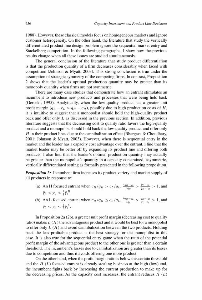
Proposition 2: Incumbent firm increases its product variety and market supply ofall products in response to:

(a) An H focused entrant when cH/qH > cL/qL, 4qH −qL

3qH>

qL−cL

qH −cH> 1, and

γ4 < γy < 13 γ H

1 .

(b) An L focused entrant when cH/qH ≤ cL/qL, 4qH −qL

3qL>

qH −cH

qL−cL> 1, and

γ5 < γy < 13 γ L

1 .

In Proposition 2a (2b), a greater unit profit margin (decreasing cost to qualityratio) makes L (H ) the advantageous product and it would be best for a monopolistto offer only L (H ) and avoid cannibalization between the two products. Holdingback the less profitable product is the best strategy for the monopolist in thiscase. It is also true for the sequential entry game when the ratio of the potentialprofit margin of the advantageous product to the other one is greater than a certainthreshold. The incumbent’s losses due to cannibalization are greater than its lossesdue to competition and thus it avoids offering one more product.

On the other hand, when the profit margin ratio is below this certain thresholdand the H (L) focused entrant is already stealing business at the high (low) end,the incumbent fights back by increasing the current production to make up forthe decreasing prices. As the capacity cost increases, the entrant reduces H (L)

Yayla-Kullu 657

Figure 1: Increasing product variety in response to H focus entrant.

production. It helps the prices to recover and provides more incentive for theincumbent to increase L (H ) production. However, when γy reaches the firstthreshold and the entrant continues to reduce production, it is not profitable forthe incumbent to further increase L (H ) production. Beyond this threshold, byoffering the entrant’s product, the incumbent steals demand which would otherwisebe satisfied by the entrant and improves its profits. As a result, the leader finds itmore profitable to introduce a product that was being held back in response to afocus strategy entrant with a high capacity investment cost. When the capacity costis much higher, beyond the second threshold, the entrant can no longer operateprofitably and ceases operations.

For example, in the airline industry, imagine a market (such as New York–Raleigh route) where a full-service carrier dominates and optimally provides anall-economy service. My results suggest that if an all-business focus carrier entersthis market and aircraft operational costs are at a high range as in Proposition 2a,it is in the best interest of the market leader airline to start offering business classseats in addition to its economy class seats.

Next, I will present an example for Proposition 2 in Figure 1. In this example,both the leader and the entrant have positive capacity costs and qH = 3.05, qL =1.5, cH = 2.5, cL = 0.9, sH = 1.5, sL = 1. I would like to show that the analyticalresults shown in the proposition continue to hold when the leader is also capacityconstrained. This example fits into Proposition 2a where the low-quality productwould be the better product and a monopolist would only offer that. However, the


example shows that the leader optimally increases its product variety in responseto an H focused entrant beyond a certain capacity cost threshold. For example,when the capacity cost of the entrant is 10 times that of the leader, only the top1.5% of the market (that is ordered by the customers’ valuations for quality) iswilling to pay for the high-quality product. Out of this 1.5%, the entrant serves1.07% and the leader serves 0.44%. The leader also offers product L and the next21.44% of the market purchases it. Note that, the graph only shows the top 5% ofthe market for brevity. At this point, it becomes a counterexample and shows thatoffering only L may not be the optimal strategy when sequential entry, productdifferentiation, and capacity costs are taken into consideration.

Stackelberg Competition with γ y ≥ γx >> 0

In this section, the second case when the leader’s cost is equally high as theentrant’s cost for capacity investment is analyzed. If an industry norm is to operatethe business via leasing of equipment and/or rental facilities such as aircraft leasingand fuel costs, then this assumption would be acceptable. Then, even an establishedfirm would have to pay the lease every month to continue operations in the marketand increases in the financial rates would affect all players equally.

Similar to the previous section, I analytically study this setting at the ex-treme case where γx = γy . After discussing analytical results, I present numericalexamples that relax this assumption. In this case, I focus more on the capacityinvestment decisions and how they are affected by the changes in capacity costs.Note that in this case optimal quantity decisions determine the necessary capacityinvestments for both firms.

The classical Stackelberg model predicts that an incumbent should ignore anentrant and keep its monopoly position in terms of market supplies. However, I findthat for a range of capacity investment cost levels, an incumbent firm may be betteroff by moving away from its monopoly position and increasing its market supplywhich necessitates an increase in its capacity investment as formally presented inthe following proposition.

Proposition 3: Suppose KM and KX are the optimal monopoly and Stackelbergleader capacity levels, respectively. Then, KX > KM in response to:

(a) An H focused entrant when cH/qH > cL/qL, sL

sH<

qL−cL

qH −cH< 1, and γ2 ≤

γy < γ6.

(b) An L focused entrant when cH/qH ≤ cL/qL, qL−cL

sL>

qH −cH

sH, and γ7 ≤

γy < γ3.

In Proposition 3a, both the increasing cost to quality ratio (cH/qH > cL/qL)and the profit margin per unit resource consumed ( qH −cH

sH<

qL−cL

sL) favor L. For

lower levels of γy , the leader optimally offers both products. As γy increases,the leader reduces the production of both products with the pressure of costlyresources. The reduction is more aggressive in the high end because H generatesless potential profit when resources consumed are taken into account. Eventually,at the first threshold for γy , the leader ceases the high-quality production altogether.

Yayla-Kullu 659

It is better to offer only L beyond this threshold. Until this point, the leader behaveslike a monopolist. It is in the best interest of the leader to ignore the entrant.

Beyond the first threshold (given in the Proposition 3a), the two firms engagein a pure asymmetric competition: the leader offers only L while the entrant offersH . At this high-capacity cost range, focusing on H is inefficient and generates lowprofits per unit resource consumed for the entrant. The incumbent has incentive toincrease the production. Note that the leader’s profit is much closer to a monopolywhen there is an H focused entrant than in the case when there is a symmetric(or L focused) entrant in the market. Moreover, due to low profit margin per unitresource consumed, the H focused entrant is affected more than the leader withthe increase in γy . As a result, the entrant reduces production more aggressivelyas γy increases. This creates additional incentive for the incumbent to increaseproduction to satisfy the demand that is left over from the entrant. As a result, therelative difference in production between a Stackelberg leader and a monopolistincreases with γy up to the second threshold. Beyond the second threshold, theentrant chooses to stay out of the market.

In Proposition 3b, while decreasing cost to quality favors H , profit marginper unit resource consumed ( qH −cH

sH<

qL−cL

sL) favors L. When γy is low enough,

the incumbent firm offers only H and has incentive to increase production due tothe pure asymmetric competition. Like the previous case, the incumbent increasesproduction to make up for the low prices and get close to the monopoly profits.This incentive decreases as γy increases and the best utilization of the expensiveresource becomes the leading economic force for the incumbent. When γy reachesthe second threshold, the incumbent starts producing L in the market, which causesa head to head competition at the low-end market. At these high levels of γy wherethe leader also offers L, it is better to ignore the entrant. The incumbent ratherconcentrates on its own resource utilization than the competition. High-capacitycost and closer competition become the legitimate economic reasons that causethe incumbent to ignore the entrant.

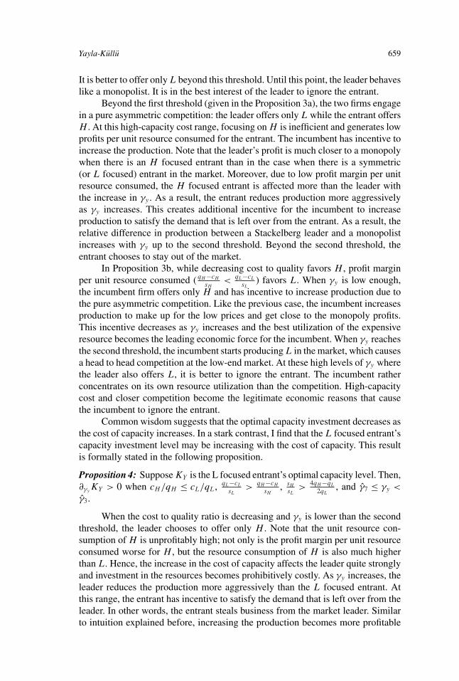
Common wisdom suggests that the optimal capacity investment decreases asthe cost of capacity increases. In a stark contrast, I find that the L focused entrant’scapacity investment level may be increasing with the cost of capacity. This resultis formally stated in the following proposition.

Proposition 4: Suppose KY is the L focused entrant’s optimal capacity level. Then,∂γy

KY > 0 when cH/qH ≤ cL/qL, qL−cL

sL>

qH −cH

sH, sH

sL>

4qH −qL

2qL, and γ7 ≤ γy <

γ3.

When the cost to quality ratio is decreasing and γy is lower than the secondthreshold, the leader chooses to offer only H . Note that the unit resource con-sumption of H is unprofitably high; not only is the profit margin per unit resourceconsumed worse for H , but the resource consumption of H is also much higherthan L. Hence, the increase in the cost of capacity affects the leader quite stronglyand investment in the resources becomes prohibitively costly. As γy increases, theleader reduces the production more aggressively than the L focused entrant. Atthis range, the entrant has incentive to satisfy the demand that is left over from theleader. In other words, the entrant steals business from the market leader. Similarto intuition explained before, increasing the production becomes more profitable


for the entrant even if the cost of investment increases. Note that this result doesnot arise when the firms are strategically symmetric as in Yayla-Kullu et al. (2013).It is an outcome of the strategic asymmetry between the competing firms.

In order to understand this result better, let’s look at a hypothetical example.Suppose that there are two airlines operating in the market between cities A and Band there are 1,000 potential customers in a given time unit. Airline X is the marketleader and its offerings are observable by Airline Y which is an all-economy classairline entrant. The market is heterogenous such that a customer with the highestquality valuation is willing to pay $3, 000 for a first class seat and $1, 000 foran economy class seat. Suppose that it costs $1, 500 to offer a first class seatwhereas it costs $600 to offer an economy class seat. These operating costs do notinclude the opportunity cost but only items such as fuel, flight attendants, service,and food. Suppose also that a first class seat occupies seven times the space ofan economy class seat. The airline industry has a wide range of seat sizes. Aneconomy class seat can be as small as 28” by 17.5”. On the other hand, a first classsuite can get as spacious as a private bedroom with a stand-alone bed, a personalfull length wardrobe, and a 23” LCD TV. In such a market, the capacity investmentcosts can be equally low for the two firms. Note that rescheduling a plane to anew route within an already existing fleet has negligible costs. Then, increasingcapacity by adding flights on a given route at a given time does not necessarilyrequire capital investment. Let’s say the capacity investment cost is γy = $0 perunit space. Then, the entrant optimally offers only 70 economy class seats. Ifthe capacity investment cost is greater, (let’s say γy = $70 per unit space), thenthe entrant offers 81 economy class seats. The entrant has increased its capacityinvestment even though the costs are more in the latter case. Note that in the lowcost case, the leader offers 260 first class seats while in the high cost case, it offers169 first class seats.

In this example, there are two forces at play for the leader. The first one isthe cannibalization concern: the leader does not offer economy class seats becausefirst class seats are very profitable. It is not good for the company to offer economyclass seats and cannibalize its own sales. The second force is the utilization ofcostly resources: the leader has to reduce the supply in the market to keep its costsat a minimum and prices as high as possible. Note that one extra first class seatcosts seven times more compared to an economy class seat due to costly resourceinvestments. This causes the leader to reduce its supply more aggressively thanthe low-quality focused entrant. In this setting, the entrant is also affected by theincreasing cost. However, the faster reduction of supply in the first class marketgenerates opportunity (through increasing prices) for the economy class market.By increasing its supply, the entrant is now able to sell more seats for higher priceswhich pays off for the increase in the capacity cost.

Similar to Figure 1, Figure 2 presents an example relaxing the leader’scapacity cost assumption for Propositions 3 and 4 when the entrant is L focused. Inthis example, the leader’s capacity costs are smaller than those of the entrant’s andqH = 3, qL = 1, cH = 1.5, cL = 0.6, sH = 7, and sL = 1. This example showsthe case where the high-quality product would be the better product for lowcapacity costs and the leader would only offer that up to a capacity cost threshold.For example, when the capacity costs are relatively lower, the leader covers the

Yayla-Kullu 661

Figure 2: Entrant’s capacity investments increasing in costs.

top 21.8% of the market by offering product H and the entrant covers the next7.2% by offering product L. When the capacity costs increase to an intermediatelevel, the leader lowers its production down to 17.7% while the entrant increases itup to 7.4%. At this point this example becomes a counterexample and shows thatincreasing capacity investments with increasing costs may indeed be the optimalstrategy when sequential entry, product differentiation, and capacity costs are takeninto consideration.

IMPLICATIONS ON QUALITY

In this section, I look at another strategy that can be put into action by the leaderin response to a focus strategy entrant. A possible change in the quality levels ofthe products when there is a threat of entry in the market is investigated. Note thatit may not always be feasible to change the quality levels of the products sincethere could be technological and/or time constraints that prevent firms utilizingthis lever.

In order to extend to endogenous quality levels, I need to define functionalforms for unit production costs and unit resource consumptions. For unit productioncosts, I follow the literature (cf. Moorthy, 1984, p. 292) and assume a quadraticfunction of quality (c(q) = αq2). For unit resource consumptions, I also assumea quadratic function (s(q) = q2) for analytical tractability. However, note that aquadratic cost function results in increasing cost to quality ratio (cH/qH > cL/qL)


and a quadratic resource consumption function results in (sH/qH > sL/qL) whichlimits the discussion only to these cases unlike the previous section.

I also limit the discussion to the cases when the market leader offers bothproducts and capacity cost is in the two extremes. This makes it possible to directour attention to the research questions about the quality choices in response to afocus strategy entrant.

A Monopolist’s Quality Decision and Capacity Investments

A monopolist that needs to make quality choices (qMi ∈ [q, q]) and capacity in-

vestments solves the following problem:

Max(pH

(xM

H , xML

) − c(qM

H

))xM

H + (pL

(xM

H , xML

) − c(qM

L

))xM

L − γxKM,

(5)

subject to s(qM

H

)xM

H + s(qM

L

)xM

L ≤ KM,

KM > 0, xMi > 0, qM

i ∈ [q, q], i = H, L.

I find that a monopolist reduces the quality levels to control the increasingcapacity cost. The characterization of this result is provided in the following lemma.It will help to discuss findings for the competitive setting.

Lemma 2: When 25q

< γx + α < 15q

, qMH = 2

5(α+γx ) , qML = 1

5(α+γx ) , xMH =

15 , xM

L = 15 .

For a large range of cost parameters, the firm optimally fixes the productionquantity at a constant level for both products. When γx increases, the monopolistreduces capacity investment through reducing the quality levels offered in themarket. A similar observation is true for the unit production cost parameter (α).An increase in α is offset by a reduction in the quality levels rather than a reductionin the production quantity.

For an airline, when the product line is fixed at two products, such as businessand economy cabins, I find that when the capacity costs are increasing, the firmoptimally reduces the overall service quality (therein customers’ willingness topay as measured by θqi).

Stackelberg Competition with γ y >> γx = 0

As in the previous section, I start by analyzing the capacity decision in two cases. Incase 1, I study the model where the leader’s capacity investment cost is lower thanthe entrant’s cost. For analytical tractability, I will study the extreme case where it iszero. On the other hand, the new entrant needs to make costly resource investmentsbefore it can start operating in the market. Then, leader firm X’s problem is revisedas follows:

Max (pH (xH , xL, yj (xH , xL)) − c(qH ))xH + (pL(xH , xL, yj (xH , xL))

−c(qL))xL,

subject to xi ≥ 0, qi ∈ [q, q], i = H, L

(6)

Yayla-Kullu 663

The entrant, firm Y’s problem is given as follows:

Max(KY ≥0,yj ≥0)

(pj (xH , xL, yj ) − c(qj ))yj − γyKY subject to s(qj )yj ≤ KY . (7)

I find that the production quantity of the high-quality product may increase asa response to an H focused entrant when the leader has no capacity constraint andunit production costs are below a certain threshold. This finding is in contrast withthe earlier papers (Ashiya, 2002; Barbot, 2008). With no consideration of eitherthe unit production costs or the capacity costs, Ashiya (2002) and Barbot (2008)suggest that the leader should exit the high-quality market when a high-qualityentry occurs. I show that optimal choices change when such operational factorsare taken into consideration.

Proposition 5: Suppose x∗i and q∗

i are the Stackelberg leader’s optimal productionquantity and quality level for i = H, L. Then, in response to an H focused entrant,q∗

i > qMi for i = H, L and x∗

L > xML when γy ≥ α > 2

5q. In addition, x∗

H > xMH

when α <2γy

3 + 25q

.

The leader has multiple incentives to increase the quality levels in this case.First, it wants to increase the prices that will be driven down due to competition.Second, the new entrant is affected more by an increase in quality due to the capacityinvestment cost. Remember in this case, the leader has a negligible capacity cost,and both the unit production costs and unit resource consumptions increase withquality. When the entrant’s cost of capacity is relatively high, the entrant choosesto reduce production due to costly capacity investments. Eventually, the leadersets the industry standard for quality to the highest level feasible and puts thenew entrant in a tough position in terms of profitability. Moreover, when the unitproduction cost parameter (α) is below a certain threshold, I show that the leaderalso increases its H production. Because the leader has no capacity investment costand this cost increases considerably for the entrant, the entrant reduces productionconsiderably. This creates incentive for the leader to increase its H production andsteal business from the entrant. The leader recovers its profits by this increase inproduction as long as the production costs remain below a certain threshold.

This result explains the behavior of AA toward EOS in the London–New Yorkroute in 2007–2008 (Rowell, 2009). The dominant airline (AA) with multipleproducts (both business class and economy class) faced a business class focusentrant (EOS) in the market. AA attacked the entrant by increasing its flightfrequency (in other words, production quantity) and by offering double frequentflier miles and new services which increase the customers’ valuations of the service(in other words, better overall quality of service). In the end, increasing financialburden due to costly resources pushed the new entrant (EOS) over the edge and itwent bankrupt before the end of 2008.

Stackelberg Competition with γ y = γx >> 0

In order to allow for the capacity decision, the leader firm X’s problem is revisedin the following and the entrant firm Y’s problem is kept as in Equation (7):


Max (pH (xH , xL, yj (xH , xL)) − c(qH ))xH

+ (pL(xH , xL, yj (xH , xL)) − c(qL))xL − γxKX, (8)

subject to s(qH )xH + s(qL)xL ≤ KX,

KX ≥ 0, xi ≥ 0, qi ∈ [q, q], i = H, L.

I find that the leader adjusts the quality levels of products, shift operationstoward the other product, and moves away from the entrant’s market. This resultis presented in the following proposition.

Proposition 6: Suppose x∗i and q∗

i are the Stackelberg leader’s optimal productionquantity and quality level for i = H, L. Then,

(a) q∗i > qM

i for i = H, L, x∗L > xM

L and x∗H < xM

H in response to an Hfocused entrant when γy + α > 2

5q.

(b) q∗i < qM

i for i = H, L, x∗L < xM

L and x∗H > xM

H in response to an Lfocused entrant, when γy + α < 1

5q.

This proposition shows that the optimal quality increases in response to anH focused entrant when capacity investment and production costs exceed a certainthreshold. Upon entry, the best response for the leader is to reduce its operationsat the high end and shift resources to the low end. The concern with the low endis that the price is much lower than its monopoly level because of the competitionif the leader ignores the entrant and keeps the same position as a monopolist (interms of both the quality and the quantity). Therefore, the leader increases thequality levels which increases the prices. The prices under competition may begreater than its monopoly level due to increased quality. Interestingly, the impactof competition may be not only the supply increase but also the price increase asformally presented in Corollary 1.

I also find that the strategy is reversed in response to an L focused entrantwhen capacity investment and production cost parameters are below a certainthreshold. Like the previous case, best reaction for the leader is to reduce itsoperations at the low end and shift resources to the high end. However, increasingH production would require substantially more resources which are very costlydue to relatively high-quality levels. For that reason, it is best for the leader toreduce the quality levels which will reduce the costs and resource consumptionlevels for H production. Although the prices are much lower than its monopolylevels, the production and capacity costs are also much lower. This helps the leaderto offset the losses due to competition.

Corollary 1: Suppose that pMi and p∗

i are the market clearing prices undermonopoly and Stackelberg game with an H focused entrant for i = H, L, re-spectively. Then, p∗

H > pMH when 1

5q> γy + α > 7

15q. Moreover, p∗

L > pML when

15q

> γy + α >√

217−520q

.

Yayla-Kullu 665

There are few empirical papers that attempt to investigate this controversialclaim of increasing prices with competition. Frank and Salkever (1997) show thatthe price increase after entry is indeed observed in practice. Their findings areconfirmed by a recent study in Regan (2008). In the airline industry, Trethewayand Kincaid (2005) refute the widely accepted belief that the hub premiums ofsome airlines are due to near-monopoly powers. Lee and Luengo-Prado (2005)find that there exist some markets where the prices are higher even when there isgreater competition. At the time of their study, Delta passengers had paid 12% lessper mile in markets to and from Salt Lake City, which is a hub where the airlineenjoys a near-monopoly power, compared to travel throughout the remainder of itsnetwork where the firm has to compete with numerous airlines.

In this article, I offer an alternative explanation to these findings. The leaderraises the quality standards in the industry when the entrant is as capable as theleader in terms of high-quality production. This increase in quality eventually leadsto an increase in prices.

I also investigate how asymmetric competition affects the total supply in themarket. I find that when the capacity investment and production costs are fairlyhigh, an H focused entrant may cause a decrease in the overall supply. This resultis formally presented in the following corollary.

Corollary 2: Suppose xMi , x∗

i , and y∗H are the monopolist’s, Stackelberg leader’s,

and the H focused entrant’s optimal production quantities for i = H, L, respec-tively. Then, x∗

H + x∗L + y∗

H < xMH + xM

L when 15q

> γy + α > 710q

.

Existing literature on symmetric competition suggests that the total supplyin the market increases and prices decrease as the number of competing firmsincreases (Gal-Or, 1983; De Fraja, 1996; Johnson & Myatt, 2006). On the contrary,this corollary shows that the total amount of production may decrease and pricesmay increase with entry when strategic asymmetries, resource consumptions ofdifferent products, and capacity investments are taken into account. This decrease insupply is mainly due to the sharp decrease in high-quality production as explainedin Proposition 6. Even the increase in low-quality production cannot offset sucha decrease and the total supply is reduced compared to its monopoly levels whenthe resources are costly and the entrant has a high-quality focus.

MANAGERIAL INSIGHTS

In this section I will synthesize the findings of the previous sections, and summarizethe managerial insights.

First of all, the proliferation lever is expected to be pulled in response to afocus strategy entrant when the capacity cost is in the low range for the leader. Theleader with low capacity cost may introduce a product that it was holding backwhen the entrant has to bear the high capacity cost and cannibalization threat isrelatively small (profit margin ratio is below a certain threshold). When the costis high for the leader, it is no longer profitable to increase variety in response to afocus strategy entrant.

Second, the production volume lever is expected to get used both whenthe capacity cost is high and when it is not. However, the extent of this use


changes as the capacity cost increases for the leader. When it is low, the productionvolume of a market leader would be nondecreasing for all parametric settings. Onthe other hand, as the capacity cost increases, changing the production volumeloses its powerful advantage. It is observed only when there is pure asymmetriccompetition with the entrant. If the entrant’s focus product is the less advantageousproduct, then it is in the best interest of the market leader (that offers only themore advantageous product) to increase its production volume compared to itsmonopoly level.

Ignoring the new focus strategy entrant surfaces as a legitimate strategy whenthe capacity cost is in the high range for the leader. The leader chooses to ignorethe entrant when it is already offering the same product as the entrant. If the leaderfaces a head to head competition with the entrant at either end of the market, thenkeeping the same position in the market is the best option for the leader.

When the leader has the opportunity to change the quality levels of theproducts, it would use this opportunity by increasing the quality levels in responseto a high-quality focused entrant both when its capacity investment cost is low andwhen it is high. When its capacity cost is low enough, I even expect the leaderto increase the production volume of both products in response to a high-qualityfocused entrant that has a high-capacity investment cost. The condition for theleader’s volume increase occurs only when the unit production costs are below acertain threshold. In response to a low-quality focused entrant, the leader with highcapacity cost decreases the quality levels in the market. The production volumelever moves in opposite directions for the two products. While the leader increasesthe high-quality production, it decreases the low-quality production.

CONCLUSIONS

In this article, I study a multiproduct firm competing with a focus strategy entrant ina vertically differentiated market. There are two products that have different quality,unit production, and unit resource consumption levels. Because the customers areheterogenous in their willingness to pay, cannibalization within the products ofthe same firm and the entrant’s business stealing actions are major concerns forthe leader. Moreover, as products may potentially consume different levels of thecostly resource, optimal resource utilization may provide a leverage as well as adisadvantage for the leader in its fight with the new entrant. Hence, the leadershould find the balance between cannibalization, business stealing, and resourceutilization forces in this competitive setting.

In the main model, the multiproduct firm is the leader and has the capabilityto produce both products. First, the leader decides how much of each productto offer in the market. Note that the leader may decide to offer only one of theproducts in a positive quantity limiting the product variety in the market. Next, thefocus strategy entrant determines its quantity and decides on its capacity. I showthat the leader may have to increase the product variety in response to a focusstrategy entrant. The parametric regions where it is optimal for the firm to offerthe entrant’s focus product in addition to the most profitable product are identified.Offering the same product is especially important when the capacity cost is highfor the entrant firm.

Yayla-Kullu 667

Interestingly, I also find that the capacity investment level of an entrant maybe increasing with the cost of capacity. When the cost to quality ratio is decreasingand the cost of capacity is below a certain threshold, the leader chooses to offeronly the high-quality product. The incentive to reduce production is greater forthe leader than for an entrant with a focus on low-quality production, as the high-quality product may consume a greater amount of the costly resource. When thelow-quality product has greater profit margin per unit resource consumed, theentrant is at a great advantage. Eventually, increasing the production becomesmore profitable for the low-quality focused entrant even if the cost of investmentincreases for a certain range of capacity costs.

I also find that when the leader has the power to set the industry standardsby deciding the quality levels, as a response to a high-quality focused entrant, theleader increases both levels of quality and production of the low-quality product,and may decrease or increase the production of the high-quality product dependingon its capacity investment cost. Moreover, when the capacity investment cost ishigh for both the entrant and the leader, the prices may increase with entry.

Like all models, this article has limitations. I consider the case when thedemand is deterministic. This enables full characterization of the best responsefunctions of both firms. It would be interesting to discuss these findings in the faceof uncertainty. Future research can extend my work further and study the impactof focus strategy competition on product variety and capacity choices when thedemand is stochastic in nature. Furthermore, following the literature, I assumed thatconsumer preferences are distributed uniformly. This makes the analysis tractable,making it possible to keep the focus on effects of costly resources on the productline and investment choices of firms. While I verified that these insights can carryover to nonuniform distributions through some numerical examples (which are notreported in this article), it would be worthwhile for future work to further studywhat happens under nonuniform distributions in general.

REFERENCES

Ashiya, M. (2002). Sequential entry in a vertically differentiated market. JapaneseEconomic Review, 53(3), 315–336.

Barbot, C. (2008). Can low cost carriers deter or accommodate entry? Transporta-tion Research Part E: Logistics and Transportation Review, 44(5), 883–893.

Bhargava, H. K., & Choudhary, V. (2001). Information goods and vertical differ-entiation. Journal of Management Information Systems, 18(2), 89–106.

Boyaci, T., & Ray, S. (2003). Product differentiation and capacity cost interactionin time and price sensitive markets. Manufacturing and Service OperationsManagement, 5(1), 18–36.

Chayet, S., Kouvelis, P., & Yu, D. Z. (2009). Product design, pricing, and ca-pacity investment in a congested production system. In S. Netessine & C.S. Tang (Eds.), Consumer-driven demand and operations management mod-els: A systematic study of information-technology-enabled sales mechanisms


(International Series in Operations Research & Management Science). NewYork, NY: Springer, 229–251.

Conlin, M., & Kadiyali, V. (2006). Entry-deterring capacity in the Texas lodg-ing industry. Journal of Economics and Management Strategy, 15(1),167–185.

De Fraja, G. (1996). Product line competition in vertically differenti-ated markets. International Journal of Industrial Organization, 14,389–414.

Dixit, A. (1980). The role of investment in entry-deterrence. The Economic Journal,90(357), 95–106.

Dunn, A. (2008). Do low-quality products affect high-quality entry? Multiproductfirms and nonstop entry in airline markets. International Journal of IndustrialOrganization, 26(5), 1074–1089.

Frank, R. G., & Salkever, D. S. (1997). Generic entry and the pricing of pharma-ceuticals. Journal of Economics and Management Strategy, 6(1), 75–90.

Gal-Or, E. (1983). Quality and quantity competition. Bell Journal of Economics,14(2), 590–600.

Geroski, P. A. (1991). Market dynamics and entry. Oxford, UK: Blackwell.

Geroski, P. A. (1995). What do we know about entry? International Journal ofIndustrial Organization, 13, 421–440.

Haruvy, E. E., Miao, D., & Stecke, K. E. (2013). Various strategies to handle can-nibalization in a competitive duopolistic market. International Transactionsin Operational Research, 20(2), 155–188.

Jing, B. (2006). On the profitability of firms in a differentiated industry. MarketingScience, 25(3), 248–259.

Johnson, J. P., & Myatt, D. P. (2003). Multiproduct quality competition: Fightingbrands and product line pruning. American Economic Review, 93(3), 748–774.

Johnson, J. P., & Myatt, D. P. (2006). Multiproduct Cournot oligopoly. RANDJournal of Economics, 37(3), 583–601.

Lee, D., & Luengo-Prado, M. J. (2005). The impact of passenger mix on reportedhub premiums in the U.S. airline industry. Southern Economic Journal, 72(2),372–394.

Lee, K. S., & Ng, I. C. L. (2007). An integrative framework of pre-emptionstrategies. Journal of Strategic Marketing, 15, 327–348.

Moorthy, K. S. (1984). Market segmentation, self-selection, and product line de-sign. Marketing Science, 3(4), 288–307.

Mussa, M., & Rosen, S. (1978). Monopoly and product quality. Journal of Eco-nomic Theory, 18, 301–317.

Neven, D. J. (1989). Strategic entry deterrence: Recent developments in the eco-nomics of industry. Journal of Economic Surveys, 3(3), 213–233.

Yayla-Kullu 669

Oster, C. V., & Strong, J. S. (2001). Predatory practices in the U.S. airline industry.Technical Report, Department of Transportation.

Regan, T. L. (2008). Generic entry, price competition, and market segmentation inthe prescription drug market. International Journal of Industrial Organiza-tion, 26, 930–948.

Rowell, D. M. (2009). Is airline competition always fair?, accessed December 13,2012, available at http://www.thetravelinsider.com/airlinemismanagement/unfaircompetition.htm.

Smiley, R. (1988). Empirical evidence on strategic entry deterrence. InternationalJournal of Industrial Organization, 6, 167–180.

Spence, A. M. (1977). Entry, capacity, investment and oligopolistic pricing. TheBell Journal of Economics, 8(2), 534–544.

Tirole, J. (1988). The theory of industrial organization. Cambridge, MA: MITPress.

Tretheway, M. W., & Kincaid, I. S. (2005). The effect of market structure on airlineprices: A review of empirical results. Journal of Air Law and Commerce, 70,467–498.

Tsikriktsis, N. (2007). The effect of operational performance and focus on prof-itability: A longitudinal study of the U.S. airline industry. Manufacturingand Service Operations Management, 9(4), 506–517.

Yayla-Kullu, H. M., Parlakturk, A. K., & Swaminathan, J. M. (2011). Segmentationopportunities for a social planner: Impact of limited resources. DecisionSciences, 42(1), 275–296.

Yayla-Kullu, H. M., Parlakturk, A. K., & Swaminathan, J. M. (2013). Multi-product quality competition: Impact of resource constraints. Production andOperations Management, 22(3), 603–614.

Yayla-Kullu, H. M., & Tansitpong, P. (2011). Allocating capacity among qualitydifferentiated products: Evidence from airline industry. Journal of Asia-Pacific Business, 12(2), 94–122.

APPENDIX A: CAPACITY COST THRESHOLDS

We define the following threshold capacity cost levels that may depend on thetype of the product i = H, L. We refer to these threshold capacity cost levels fordescribing the firms’ optimal policies.

γ i1 = qi − ci

si

, (A1)

γ2 = qH − cH − qL + cL

sH − sL

, (A2)

γ3 = cLqH − cHqL

qLsH − qH sL

, (A3)


γ4 = qH (qL − cL − (qH − cH ))

(qH − qL)sH

, (A4)

γ5 = cLqH − cHqL

(qH − qL)sL

, (A5)

γ6 = qH (2cL + 4qH − 3qL) + cH (−4qH + qL)

4qH sH − qLsH − 2qH sL

, (A6)

γ7 = 4cLqH − 2cHqL − cLqL − 2qHqL + q2L

2qLsH − 4qH sL + qLsL

. (A7)

APPENDIX B: PROOFS

Proof of Lemma 1: Following the main model, demands for the two producttypes are given as DH (pL, pH ) = 1 − pH −pL

qH −qL, and DL(pL, pH ) = pH −pL

qH −qL− pL

qL.

Then prices are set to clear the market based on the total amount of production inthe industry: pH (xH , xL, yj ) and pL(xH , xL, yj ).

Following the fact that xi + yi = Di(pH , pL), the above price–quantity equa-tions can be solved for prices as follows: pH = qH (1 − xH − yH ) − qLxL andpL = qL(1 − xL − xH − yH ) for the high-quality entrant and pH = qH (1 − xH ) −qL(xL + yL) and pL = qL(1 − xL − yL − xH ) for the low-quality entrant.

For the leader against a high-quality entrant, ∂xH ,xH((qH (1 − xH −

yH ) − qLxL − cH )xH + (qL(1 − xL − xH − yH ) − cL)xL − γxKX) = −2qH

and ∂xL,xL((qH (1 − xH − yH ) − qLxL − cH )xH + (qL(1 − xL − xH − yH ) −

cL)xL − γxKX) = −2qL and ∂xH ,xL((qH (1 − xH − yH ) − qLxL − cH )xH +

(qL(1 − xL − xH − yH ) − cL)xL − γxKX) = −2qL and ∂KX,KX((qH (1 − xH −

yH ) − qLxL − cH )xH + (qL(1 − xL − xH − yH ) − cL)xL − γxKX) = 0. For thehigh-quality entrant, ∂yH ,yH

((qH (1 − xH − yH ) − qLxL − cH )yH − γyKY ) =−2qH and ∂KY ,KY

((qH (1 − xH − yH ) − qLxL − cH )yH − γyKY ) = 0.For the leader against a low-quality entrant, ∂xH ,xH

((qH (1 − xH ) −qL(xL + yL) − cH )xH + (qL(1 − xL − yL − xH ) − cL)xL − γxKX) = −2qH

and ∂xL,xL((qH (1 − xH ) − qL(xL + yL) − cH )xH + (qL(1 − xL − yL − xH ) −

cL)xL − γxKX) = −2qL and ∂xH ,xL((qH (1 − xH ) − qL(xL + yL) − cH )xH +

(qL(1 − xL − yL − xH ) − cL)xL − γxKX) = −2qL and ∂KX,KX((qH (1 − xH ) −

qL(xL + yL) − cH )xH + (qL(1 − xL − yL − xH ) − cL)xL − γxKX) = 0. For thelow-quality entrant, ∂yL,yL

((qL(1 − xL − yL − xH ) − cL)yL − γyKY ) = −2qL

and ∂KY ,KY((qL(1 − xL − yL − xH ) − cL)yL − γyKY ) = 0.

Hence, objective functions given in problems (2) and (3) are jointly concavein their corresponding decision variables. �Proof of Proposition 1: Following the price–demand equations (1) and the factthat xi = Di(pH , pL), these equations can be solved for prices as follows: pH =qH (1 − xH ) − qLxL and pL = qL(1 − xL − xH ). Note that the capacity constraintis always satisfied by equality at the optimal solution (sHxH + sLxL = KX). Weplug in this fact and price functions in the objective function. The resulting objective

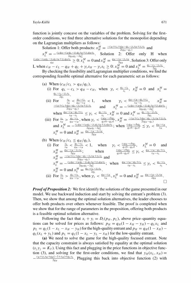
Yayla-Kullu 671

function is jointly concave on the variables of the problem. Solving for the first-order conditions, we find three alternative solutions for the monopolist dependingon the Lagrangian multipliers as follows:

Solution 1: Offer both products: xMH = −cH +cL+qH −qL−γxsH +γxsL

2(qH −qL) and

xML = − cLqH −cH qL−γxqLsH +γxqH sL

2qH qL−2q2L

. Solution 2: Offer only H whencLqH −cH qL−γxqLsH +γxqH sL

qH≥ 0: xM

L = 0 and xMH = qH −cH −γxsH

2qH. Solution 3: Offer only

L when cH − cL − qH + qL + γxsH − γxsL ≥ 0: xMH = 0 and xM

L = qL−cL−γxsL

2qL.

By checking the feasibility and Lagrangian multiplier conditions, we find thecorresponding feasible optimal alternative for each parametric set as follows:

(a) When (cH/cL > qH/qL),(i) For qL − cL > qH − cH , when γx <

qL−cL

sL, xM

H = 0 and xML =

qL−cL−γxsL

2qL.

(ii) For sL

sH<

qL−cL

qH −cH< 1, when γx <

qH −cH −qL+cL

sH −sL, xM

H =−cH +cL+qH −qL−γxsH +γxsL

2(qH −qL) and xML = − cLqH −cH qL−γxqLsH +γxqH sL

2qH qL−2q2L

;

when qH −cH −qL+cL

sH −sL≤ γx <

qL−cL

sL, xM

H = 0 and xML = qL−cL−γxsL

2qL.

(iii) For sL

sH>

qL−cL

qH −cH, when γx <

clqH −chqL

qlsh−qhsl, xM

H = −cH +cL+qH −qL−γxsH +γxsL

2(qH −qL)

and xML = − cLqH −cH qL−γxqLsH +γxqH sL

2qH qL−2q2L

; when clqH −chqL

qlsh−qhsl≤ γx <

qH −cH

sH,

xML = 0 and xM

H = qH −cH −γxsH

2qH.

(b) When (cH/cL ≤ qH/qL),(i) For sL

sH<

qL−cL

qH −cH< 1, when γx <

clqH −chqL

qlsh−qhsl, xM

L = 0 and

xMH = qH −cH −γxsH

2qH; when clqH −chqL

qlsh−qhsl≤ γx <

qH −cH −qL+cL

sH −sL,

xMH = −cH +cL+qH −qL−γxsH +γxsL

2(qH −qL) and

xML = − cLqH −cH qL−γxqLsH +γxqH sL

2qH qL−2q2L

; when qH −cH −qL+cL

sH −sL≤ γx <

qL−cL

sL,

xMH = 0 and xM

L = qL−cL−γxsL

2qL.

(ii) For sL

sH>

qL−cL

qH −cH, when γx <

qH −cH

sH, xM

L = 0 and xMH = qH −cH −γxsH

2qH.

�Proof of Proposition 2: We first identify the solutions of the game presented in ourmodel. We use backward induction and start by solving the entrant’s problem (3).Then, we show that among the optimal solution alternatives, the leader chooses tooffer both products over others whenever feasible. The proof is completed whenwe show that for the range of parameters in the proposition, offering both productsis a feasible optimal solution alternative.

Following the fact that xi + yi = Di(pH , pL), above price–quantity equa-tions can be solved for prices as follows: pH = qH (1 − xH − yH ) − qLxL andpL = qL(1 − xL − xH − yH ) for the high-quality entrant and pH = qH (1 − xH ) −qL(xL + yL) and pL = qL(1 − xL − yL − xH ) for the low-quality entrant.

(a) We need to solve the game for the high-quality focused entrant. Notethat the capacity constraint is always satisfied by equality at the optimal solution(sjyj = KY ). Using this fact and plugging in the price functions in objective func-tion (3), and solving for the first-order conditions, we find that yH (xL, xH ) =− cH +γysH +qH (−1+xH )+qLxL

2qH. Plugging this back into objective function (2) with


γx = 0, and solving for the first-order conditions, we find three alternative so-lutions for the leader depending on the Lagrangian multipliers as follows:

Solution 1: Offer both products: xH = −cH qH +cLqH +(qH −qL)(qH +γysH )2qH (qH −qL) , xL =

− cLqH −cH qL

2qH qL−2q2L

. Solution 2: Offer only H when cL − cH qL

qH≥ 0: xH =

−cH +qH +γysH

2qH, xL = 0. Solution 3: Offer only L when cH qH −cLqH −(qH −qL)(qH +γysH )

2qH −qL≥

0: xH = 0, xL = −−2cLqH +qL(cH +qH +γysH )2qL(−2qH +qL) .

Then, we plug in these options one by one and calculate the profits for theleader as follows:

Profit with Solution 1: π1

= 2c2Lq2

H −4cH cLqH qL+qL(c2H (qH +qL)−2cH (qH −qL)(qH +γysH )+(qH −qL)(qH +γysH )2)

8qH (qH −qL)qL.

Profit with Solution 2: π2 = (−cH +qH +γysH )2

8qH.

Profit with Solution 3: π3 = (−2cLqH +qL(cH +qH +γysH ))2

8qH (2qH −qL)qL.

Since qH > qL, π1 − π2 = (cLqH −cH qL)2

4qH (qH −qL)qL> 0 and π1 − π3 =

(−cH qH +cLqH +(qH −qL)(qH +γysH ))2

4qH (2q2H −3qH qL+q2

L)> 0.

For the conditions presented in Proposition 2a, offering both prod-ucts (Solution 1) is a feasible optimal solution alternative (xH =−cH qH +cLqH +(qH −qL)(qH +γysH )

2qH (qH −qL) > 0, xL = − cLqH −cH qL

2qH qL−2q2L

> 0). As this is the most prof-itable option, Solution 1 is the optimal best response for the leader under theconditions presented in Proposition 2a. Following Proposition 1a part (i), the mo-nopolist’s optimal product line would be offering only L for the same conditionswhich completes the proof for Proposition 2a.

(b) Following similar steps, we solve the game for the low-quality focusedentrant. Plugging in the price functions in objective function (3), and solving for thefirst-order conditions, we find that yL(xL, xH ) = − cL+γysL+qL(−1+xH +xL)

2qL. Plugging

this back into objective function (2), and solving for the first-order conditions,we find three alternative solutions for the leader depending on the Lagrangianmultipliers as follows:

Solution 1: Offer both products: xH = −cH +cL+qH −qL

2(qH −qL) , xL =−cLqH +cH qL+γy (qH −qL)sL

2(qH −qL)qL. Solution 2: Offer only H when cLqH −cH qL+γy (−qH +qL)sL

2qH −qL≥ 0:

xH = −2cH +cL+2qH −qL+γysL

4qH −2qL, xL = 0. Solution 3: Offer only L when

cH − cL − qH + qL ≥ 0: xH = 0, xL = −cL+qL+γysL

2qL.

Then, we plug in these options one by one and calculate the profits for theleader as follows: Profit with Solution 1:

π1 =(2c2

H qL−4cH cLqL+c2L(qH +qL)+2cL(qH −qL)(qL−γysL)+(qH −qL)(−qL(4cH −2qH +qL)+2γyqLsL+γ 2

y s2L))

8(qH −qL)qL.

Profit with Solution 2: π2 = (−2cH +cL+2qH −qL+γysL)2

16qH −8qL.

Profit with Solution 3: π3 = (−cL+qL+γysL)2

8qL.

Since qH > qL, π1 − π2 = (cLqH −cH qL+γy (−qH +qL)sL)2

4qL(2q2H −3qH qL+q2

L)> 0 and π1 − π3 =

(cH −cL−qH +qL)2

4(qH −qL) > 0.

Yayla-Kullu 673

For the conditions presented in Proposition 2b, offering both products (So-lution 1) is a feasible optimal solution alternative (xH = −cH +cL+qH −qL

2(qH −qL) > 0 and

xL = −cLqH +cH qL+γy (qH −qL)sL

2(qH −qL)qL> 0). Because this is the most profitable option, So-

lution 1 is the optimal best response for the leader under the conditions presentedin the Proposition 2b. Following Proposition 1b, the monopolist’s optimal productline would be offering only H for the same conditions which completes the proof.

Next we show how the quantities are also increasing:

(a) The high-quality focused entrant’s best response is yH = −((cH +γysH + qH (−1 + xH ) + qLxL)/(2qH )). Then, by solving the first-orderconditions and checking for feasibility conditions, the leader’s best re-sponse is characterized and compared to the monopolist’s solution asfollows:when 4qH −qL

3qH>

qL−cL

qH −cH, for qH (qL−cL−(qH −cH ))

(qH −qL)sH< γy ≤ qH −cH

3sH,

x∗H = (−cH qH +cLqH +(qH −qL)(qH +γysH ))

(2qH (qH −qL)) > xMH , x∗

L = − cLqH −cH qL

2qH qL−2q2L

> xML .

(b) The low-quality focused entrant’s best response is yL = −((cL + γysL +qL(−1 + xH + xL))/(2qL)). Then, by solving the first-order conditionsand checking for feasibility conditions, the leader’s best response ischaracterized and compared to the monopolist’s solution as follows:when 4qH −qL

3qL>

qH −cH

qL−cL, for cLqH −cH qL

(qH −qL)sL< γy ≤ qL−cL

3sL,

x∗H = (−cH + cL + qH − qL)/(2(qH − qL)) > xM

H , x∗L = (−cLqH +

cHqL + γy(qH − qL)sL)/(2(qH − qL)qL) > xML . �

Proof of Proposition 3: We first solve the game and identify leader’s and follower’sactions for the parametric sets presented in the proposition. Then, we compare themwith the monopolist’s solution as presented in Proposition 1. Following the factthat xi + yi = Di(pH , pL), price–demand equations (1) can be solved for pricesas follows: pH = qH (1 − xH − yH ) − qLxL and pL = qL(1 − xL − xH − yH ) forthe high-quality entrant and pH = qH (1 − xH ) − qL(xL + yL) and pL = qL(1 −xL − yL − xH ) for the low-quality entrant. Note that the capacity constraint isalways satisfied by equality at the optimal solution for both firms(sjyj = KY andsHxH + sLxL = KX).

(a) We solve the game for the high-quality focused entrant. Pluggingin the capacity and price functions in objective function (3), andsolving for the first-order conditions, we find that yH (xL, xH ) =− cH +γysH +qH (−1+xH )+qLxL

2qH. Plugging this back into objective function (2),

and solving for the first-order conditions, we find three alternative solu-tions for the leader depending on the Lagrangian multipliers as follows:Solution 1: Offer both products: xH = −cH +cL+qH −qL−γysH +γysL

2(qH −qL) and

xL = − cLqH −cH qL−γyqLsH +γyqH sL

2qH qL−2q2L

.

Solution 2: Offer only H when cLqH −cH qL−γyqLsH +γyqH sL

qH≥ 0: xL = 0 and

xH = qH −cH −γysH

2qH.

Solution 3: Offer only L when qH (cH −cL−qH +qL+γysH −γysL)2qH −qL

≥ 0: xH = 0and


xL = −−2cLqH +cH qL+qH qL+γyqLsH −2γyqH sL

−4qH qL+2q2L

.We find that Solution 3 is the only feasible optimal alterna-tive when cH/qH > cL/qL, sL

sH<

qL−cL

qH −cH< 1, and (qH −cH )−(qL−cL)

sH −sL≤

γy <−2cLqH +(cH +qH )qL

−qLsH +2qH sL. Solving for optimal yH , we find yH =

2cLqH +4q2H −3qH qL+cH (−4qH +qL)−4γyqH sH +γyqLsH +2γyqH sL

4qH (2qH −qL) that requires

γy <qH (2cL+4qH −3qL)+cH (−4qH +qL)

4qH sH −qLsH −2qH sL(< −2cLqH +(cH +qH )qL

−qLsH +2qH sL).

Then, xL > xML ⇒ KX∗ > KM when (qH −cH )−(qL−cL)

sH −sL< γy , which com-

pletes the proof for Proposition 3a.

(b) We solve the game for the low-quality focused entrant. Plugging inthe capacity equality and price functions in objective function (3),and solving for the first-order conditions, we find that yL(xL, xH ) =− cL+γysL+qL(−1+xH +xL)

2qL. Plugging this back into objective function (2),

and solving for the first-order conditions, we find three alternative solu-tions for the leader depending on the Lagrangian multipliers as follows:Solution 1: Offer both products: xH = −cH +cL+qH −qL−γysH +γysL

2(qH −qL) and

xL = − cLqH −cH qL−γyqLsH +γyqH sL

2qH qL−2q2L

.

Solution 2: Offer only H when cLqH −cH qL−γyqLsH +γyqH sL

2qH −qL≥ 0: xL = 0 and

xH = −2cH +cL+2qH −qL−2γysH +γysL

4qH −2qL.

Solution 3: Offer only L when cH − cL − qH + qL + γysH − γysL ≥ 0:xH = 0 and xL = − cL−qL+γysL

2qL.

We find that Solution 2 is the only feasible optimal alternative whencH/qH ≤ cL/qL, qL−cL

sL>

qH −cH

sH, and γy ≤ cLqH −cH qL

qLsH −qH sL.

Solving for optimal yL, we find yL =− cL+γysL+(qL(−2cH +cL−2qH +qL−2γysH +γysL))/(4qH −2qL)

2qLthat requires

γy >4cLqH −2cH qL−cLqL−2qH qL+q2

L

2qLsH −4qH sL+qLsL.

Then, xH > xMH ⇒ KX∗ > KM when γy <

cLqH −cH qL

qLsH −qH sLwhich completes

the proof. �

Proof of Proposition 4: Following the proof of Proposition 3b,when cH/qH ≤ cL/qL, qL−cL

sL>

qH −cH

sH, and γy ≤ cLqH −cH qL

qLsH −qH sL, optimal yL =

− cL+γysL+(qL(−2cH +cL−2qH +qL−2γysH +γysL))/(4qH −2qL)2qL

that requires γy >4cLqH −2cH qL−cLqL−2qH qL+q2

L

2qLsH −4qH sL+qLsL. Then, we take the deriva-

tive of KY = sLyL with respect to capacity cost parameter γy : ∂γyKY =

− sL(sL+(qL(−2sH +sL))/(4qH −2qL))2qL

which is positive when sH

sL>

4qH −qL

2qL. �

Proof of Lemma 2: Following the price–demand equations (1) andthe fact that xi = Di(pH , pL), these equations can be solved for pricesas follows: pH = qH (1 − xH ) − qLxL and pL = qL(1 − xL − xH ). Notethat the capacity constraint is always satisfied by equality at theoptimal solution (s(qH )xH + s(qL)xL = KX). We plug this fact, price,and cost functions into the objective function. The resulting problemis as follows: πM = xH (qH (1 − xH ) − qLxL − αq2

H ) + xL(qL(1 − xH − xL) −

Yayla-Kullu 675

αq2L) − γx(q2

HxH + q2LxL). Hessian (πM ) = {{−2qH , −2qL}, {−2qL, −2qL}}. Be-

cause this is negative definite, we use first-order conditions to find the optimal{xH (qH , qL), xL(qH , qL)} which yields: xL = (1/2)qH (γx + α), xH = 1/2(1 −γxqH − γxqL − qHα − qLα). We continue by plugging the optimal quantities backin the profit function and solving for the optimal quality levels.

πM = (1/4)qH (1 + (γx + α)(q2H (γx + α) − q2

L(γx + α) + qH (−2 +qL(γx + α)))). This function is strictly concave in qL since ∂qL,qL

πM =−(1/2)qH (γx + α)2. Then, we use first-order conditions to find the optimalqL = qH/2. We continue by plugging it back in the profit function and solving forthe optimal qH .

πM = (1/4)qH (1 + 1/4qH (γx + α)(−8 + 5γxqH + 5qHα)). ∂qH ,qHπM =

1/8(γx + α)(−8 + 15qH (γx + α)). Then, we need to double check the criticalpoint to find out the optimal solution. Solving for the first-order conditions, wefind two critical points (qH = 2/(5(γx + α)), qH = 2/(3(γx + α))) in addition tothe boundary conditions (qL ≥ q and qH ≤ q).

For the conditions presented in Lemma 2, we find that qMH = 2/(5(γx + α)) is

the unique global maximum point. Then, qML = 1

5(α+γx ) , xMH = 1

5 , xML = 1

5 , pMH =

725(α+γx ) , p

ML = 3

25(α+γx ) , πM = 1

25(α+γx ) . �

Proof of Proposition 5: We solve the game and identify leader’s and follower’sactions for the parametric sets presented in the proposition. Then, we comparethem with the monopolist’s solution as presented in Lemma 2.

Plugging in (s(qH )yH = KY ) and the price–demand equations (1) into Equa-tion (7), and solving for the first-order conditions, we find that yH (xL, xH ) =− qLxL+qH (−1+xH +qH (γy+α))

2qH. We plug yH (xL, xH ), price, and cost functions in Equa-

tion (6). The resulting problem is as follows: πUH = ( 12qH

)(q2Lx2

L + q3HxH (γy −

α) − qHqLxL(−1 + 2xH + 2xL + 2qLα) + q2H (xH − x2

H + qLxL(γy + α))). Wesolve the problem sequentially: first we find optimal quantities taking qualitylevels qH and qL as given. Then, we plug them in and solve for the optimal qual-ity levels. First, we find the Hessian (πUH ) = {{−qH , −qL}, {−qL, (−4qHqL +2q2

L)/(2qH )}}. It is negative definite if q∗H > 3/2 q∗

L. We will verify this conditionlater.

We continue by solving first-order conditions to find the optimal{xH (qH , qL), xL(qH , qL)} which yields xL = (qHα)/2, xH = 1/2(1 + γyqH −qHα − qLα). We continue by plugging the optimal quantities back into the profitfunction and solving for the optimal quality levels.

πUH = (1/8) qH ((1 + γyqH )2 − 2qH (1 + γyqH )α + (q2H + 2qHqL −

2q2L)α2). This function is strictly concave in qL since ∂qL,qL

πUH = −((qHα2)/2).Then, we use first-order conditions to find the optimal qL = qH/2. Here we verifythe condition on the Hessian since qH = 2qL > 3/2 qL. We continue by pluggingit back into the profit function and solving for the optimal qH .

πUH = (1/8) qH ((1 + γyqH )2 − 2qH (1 + γyqH )α + (3q2Hα2)/2). We next

show that this function is everywhere increasing (derivative with respect to qH

is positive for all qH ) for γy ≥ α which proves that the maximum is achieved atthe boundary condition.


∂qHπUH = (1/16) (2 + qH (6γ 2

y qH + γy(8 − 12qHα) + α(−8 + 9qHα))) =2 + 8qH (γy − α) + q2

H (6(γy − α)2 + 3α2) > 0 for all qH when γy ≥ α aspresented in the proposition. Hence, q∗

H = q > qMH .

Solving all functions backwards and comparing the results with Lemma2, we find q∗

L = q/2(> qML ), x∗

H = (1/4) (2 + q(2γy − 3α)) (> xMH only if α <

2γy

3 + 25q

), x∗L = (qα)/2(> xM

L ). �

Proof of Proposition 6: We solve the game and identify the leader’s and follower’sactions for both types of entrants as presented in the proposition. Then we comparethem with the monopolist’s solution as presented in Lemma 2.

(a) We solve the game for the high-quality focused entrant. Plugging(s(qH )yH = KY ) and the price functions from Equation (1) intoEquation (7), and solving for the first-order conditions, we findthat yH (xL, xH ) = −((qLxL + qH (−1 + xH + qH (γy + α)))/(2qH )).We plug in yH (xL, xH ), capacity (s(qH )xH + s(qL)xL = KX), price,and cost functions in Equation (8). The resulting problem is asfollows: πKH = (1/2qH )(q2

Lx2L − q3

HxH (γy + α) − qHqLxL(−1 +2γyqL + 2xH + 2xL + 2qLα) + q2

H (xH − x2H + qLxL(γy + α))).

We solve the problem sequentially: first we find optimal quan-tities taking quality levels qH and qL as given. Then, weplug them in and solve for the optimal quality levels. Hessian(πKH ) = {{−qH , −qL}, {−qL, (−4qHqL + 2q2

L)/(2qH )}}. It is negativedefinite if q∗

H > 3/2 q∗L. We will verify this condition later.

We continue by solving first-order conditions to find the opti-mal {xH (qH , qL), xL(qH , qL)} which yields xL = 1/2qH (γy + α), xH =1/2(1 − (qH + qL)(γy + α)). We continue by plugging the optimal quan-tities back into the profit function and solving for the optimal qualitylevels.πKH = (1/8)qH (1 − 2qH (γy + α) + (q2

H + 2qHqL − 2q2L)(γy + α)2).

This function is strictly concave in qL since ∂qL,qLπKH =

−((qH (γy + α)2)/2). Then, we use first-order conditions to findthe optimal qL = qH/2. Here we verify the condition on the Hessiansince qH = 2qL > 3/2 qL. We continue by plugging it back in the profitfunction and solving for the optimal qH .πKH = (1/16)(qH (2 − 4qH (γy + α) + 3q2

H (γy + α)2)). We next showthat this function is everywhere increasing (derivative with respect to qH

is positive for all qH ) which proves that the maximum is achieved at theboundary condition.∂qH

πKH = (1/16)(2 + qH (γy + α)(−8 + 9qH (γy + α))). Replace a =qH (γy + α), then proving F (a) = 2 + a(9a − 8) is positive for all a

is enough. Since F (a) is a strictly convex function, we can find thatminimum value is achieved at a = 4/9 with F (4/9) = 2/9 > 0. ThenF (a) > 0 for all a, which shows that ∂qH

πKH > 0 for all qH , whichshows that πKH is everywhere increasing. Hence, q∗

H = q > qMH when

γy + α > 25q

.

Yayla-Kullu 677

Solving all functions backwards and comparing the results with Lemma2 when γy + α > 2

5q, we find q∗

L = q/2 (> qML ), x∗

H = (1/4) (2 −3q(γy + α)) (< xM

H ), x∗L = (1/2) (q(γy + α)) (> xM

L ).

(b) We solve the problem for low-quality focused entrant. Plug-ging (s(qL)yL = KY ) and price functions from equation (1) intoEquation (7), and solving for the first-order conditions, we findthat yL(xL, xH ) = (1/2)(1 − γyqL − xH − xL − qLα). We plug inyL(xL, xH ), capacity (s(qH )xH + s(qL)xL = KX), price, and costfunctions in Equation (8). The resulting problem is as follows:πKL = (1/2)(−2qH (−1 + xH )xH − 2q2

HxH (γy + α) + qL(x2H +

xH (−1 + γyqL − 2xL + qLα) − xL(−1 + γyqL + xL + qLα))).We solve the problem sequentially: first we find optimal quan-tities taking quality levels qH and qL as given. Then, weplug them in and solve for the optimal quality levels. Hessian(πKL) = {{1/2(−4qH + 2qL), −qL}, {−qL, −qL}}. It is negativedefinite.We continue by solving first-order conditions to find the opti-mal {xH (qH , qL), xL(qH , qL)} which yields xL = 1/2qH (γy + α), xH =1/2(1 − (qH + qL)(γy + α)). We continue by plugging the optimal quan-tities back in the profit function and solving for the optimal quality levels.πKL = (1/8)(2q3

H (γy + α)]2 + 2q2H (γy + α)(−2 + qL(γy + α)) −

qL(−1 + qL(γy + α)2 + qH (2 − 2q2L(γy + α)2)). We check the con-

cavity of πKL with respect to xH . ∂qH ,qHπKL = (1/2)(γy + α)(−2 +

3qH (γy + α) + qL(γy + α)) < 0 only if (γy + α) < 2/(3q∗H + q∗

L). Wewill verify this condition later. Next, we use first-order conditions tofind the optimal qH = (1 + qL(γy + α))/(3(γy + α)) which ensuresthe feasibility (qH > qL) and concavity conditions are satisfied. Wecontinue by plugging it back into the profit function and solving for theoptimal qL.πKL = (1/(216(γy + α)))(8 − 21qL(γy + α) + 42q2

L(γy + α)2 −37q3

L(γy + α)3). We next show that this function is everywhere decreas-ing (derivative with respect to qL is negative for all qL) which provesthat the maximum is achieved at the boundary condition.∂qL

πKL = (1/72)(−7 + qL(γy + α)(28 − 37qL(γy + α))). Replace a =qL(γy + α), then proving F (a) = −7 + a(28 − 37a) is negative for alla is enough. Since F (a) is a strictly concave function, we can find thatmaximum value is achieved at a = 14/37 with F (14/37) = −63/37 <

0. Then F (a) < 0 for all a, which shows that ∂qLπKL < 0 for all qL,

which shows that πKL is everywhere decreasing. Hence, q∗L = q < qM

L

when γy + α < 15q

.

Solving all functions backwards and comparing the results with Lemma

2 when γy + α < 15q

, we find q∗H = 1+q(γy+α)

3(γy+α) < qMH , x∗

H = (1/3) (1 −2q(γy + α)) > xM

H , x∗L = (1/6) (1 + q(γy + α)) < xM

L . �


Proof of Corollary 1: We compare the solutions for the Stackelberg gameas presented in the proof of Proposition 6 and the monopolist’s solution aspresented in Lemma 2. Remember that when γy + α > 2

5q, p∗

H = (1/4)q(1 +3q(γy + α)); p∗

L = (1/8)q(1 + 2q(γy + α)) and when 25q

< γy + α < 15q

, pMH =

7/(25(γy + α)); pML = 3/(25(γy + α)).

We first test whether p∗H > pM

H . It requires 1/4q(1 + 3q(γy + α)) >

7/(25(γy + α)). When we replace q(γy + α) = β, the condition reducesto 3β2 + β − (28/25) > 0 ⇒ (β + (4/5))(β − (7/15)) > 0 ⇒ β > 7/15 ⇒(γy + α) > 7/(15q). Combining all conditions on γy and α yields the conditionin the corollary.

Next we test whether p∗L > pM

L . It requires (1/8)q(1 + 2q(γy + α)) >

3/(25(γy + α)). When we replace q(γy + α) = β, the condition reduces to2β2 + β − (24/25) > 0 ⇒ (β + (1/20)(5 + √

217))(β − (1/20)(√

217 − 5)) >

0 ⇒ β > (1/20)(√

217 − 5)) ⇒ (ck + α) > (1/20q)(√

217 − 5)). Combining allconditions on γy and α yields the condition in the corollary. �Proof of Corollary 2: We compare the solutions for the Stackelberg gameas presented in the proof of Proposition 6 and the monopolist’s solution aspresented in Lemma 2. Remember that when γy + α > 2

5q, x∗

H = (1/4) (2 −3q(γy + α)), x∗

L = (1/2) (q(γy + α)), and y∗H = 1/4 (1 − q(γy + α)). Remem-

ber that when 25q

< γy + α < 15q

, xMH = 1

5 and xML = 1

5 .

x∗H + y∗

H + x∗L < xM

H + xML when 10q(γy + α) > 7. Combining all condi-

tions on γy and α yields the condition in the corollary. �

Capacity Investment and Product Line Decisions of a ...646 Capacity Investment and Product Line...

Documents

Transcript of Capacity Investment and Product Line Decisions of a ...646 Capacity Investment and Product Line...