Risky investment decisions: How are individuals influenced ... · Risky investment decisions: How...

Risky investment decisions: How are individualsinfluenced by their groups?

W. Kip Viscusi & Owen R. Phillips & Stephan Kroll

Published online: 23 July 2011# Springer Science+Business Media, LLC 2011

Abstract We investigate the effect of group versus individual decision-making inthe context of risky investment decisions in which all subjects are fully informedof the probabilities and payoffs. Although there is full information, the lotterychoices pose cognitive challenges so that people may not be sure of theirexpected utility-maximizing choice. Making such decisions in a group contextprovides real-time information in which group members can observe others’choices and revise their own decisions. Our experimental results show thatsimply observing what others in the group do has a significant impact onbehavior. Coupling real-time information with group decisions based on themedian value, i.e., majority rule, makes the median investment choice focal,leading people with low values to increase investments and those with highvalues to decrease investments. Group decisions based on the minimuminvestment amount produce more asymmetric effects.

Keywords Real-time information . Group decisions . Experiments . Herding

JEL classification D03 . D80 . D70

J Risk Uncertain (2011) 43:81–106DOI 10.1007/s11166-011-9123-3

Research support from the Paul Lowham endowment is gratefully acknowledged. Any opinions, findings,conclusions, or recommendations expressed in this paper are those of the authors and do not necessarilyreflect the views of the funding source. Jinghui Lim provided excellent research assistance.

W. K. Viscusi (*)Vanderbilt University Law School, 131 21st Avenue South, Nashville, TN 37203-1181, USAe-mail: [email protected]

O. R. PhillipsDepartment of Economics & Finance, University of Wyoming, Laramie, WY 82071-3985, USAe-mail: [email protected]

S. KrollDepartment of Agricultural and Resource Economics, Colorado State University, Fort Collins, CO80523-1172, USAe-mail: [email protected]

Risky decisions typically do not involve isolated choices among abstract lotteries.Rather, there is often the opportunity to make an investment that affects the lotterystructure. This additional element of choice increases the cognitive challenges posedby the risky decision, making it more difficult to ascertain the optimal choice. Thisarticle examines these individual decisions when made in a group context. Unlikeexisting treatments of herding effects, there is full information about probabilitiesand payoffs. The remaining uncertainty is with respect to individual preferences inthe face of a complex task. Observing decisions by others in a group can potentiallyprovide guidance with respect to the optimal choice. This article utilizes a series ofexperiments to explore this phenomenon.

Decisions that involve risk and require up-front investments often are made in agroup environment. Examples abound. Families make down payments and financeimprovements on their residence; they decide how much to spend and where to sendchildren for their education; they save for retirement. Non-profit and for-profitboards approve major employment contracts, undertake new capital projects, andacquire other organizations or companies. Potentially large numbers of people voteon regulating business activity and funding community development. And in thecontext of our experimental design, groups consider whether to engage in litigation,where the cost of litigation is paid before the outcome is known. In general, riskyfinancial decisions are arguably more prevalent in group environments than whenindividuals make decisions in isolation.

While the difference in decision-making behavior between groups and individualshas recently been the subject of much academic research, relatively little is knownabout group behavior in which there is an investment component to the riskydecision. Individuals may act differently because of the separate and related effectsof (1) being embedded in a group and (2) the group decision rule. Most theoreticaland empirical models of risky decision-making assume that the decision-makinggroup acts as a rational economic agent, without taking group informationaldynamics and decision-making rules into account.

This article seeks to fill this void by presenting experimental evidence thatilluminates how a group environment affects risky decisions. Individual investmentdecisions that affect the lottery structure are compared to those made in threedifferent group environments in which the group faces the same range of riskyinvestments as the individual. In each group context, participants have real-timeinformation (RTI) that enables them to observe the desired investment amounts ofothers, and they can revise their investment recommendations based on theseobservations. Both RTI alone and the group decision rule—deciding how much toinvest either based on the median value (as in majority rule) or the minimum value(as in unanimous rule)—may influence individual choices. The experimental designallows us to distinguish the separate effects of simply observing what others want todo and the group decision rule, track how people change, and test for significance.

Our experiment involves the choice of an investment amount, where higherinvestment levels at first increase the chance of obtaining a higher payoff, but after apoint greater investment levels reduce the net expected payoff. To operationalize theinvestment decision in both an individual and group setting, we construct a decisioncontext that makes people contemplate filing a lawsuit. In our scenarios, up-frontinvestments must be made to earn an uncertain return.

82 J Risk Uncertain (2011) 43:81–106

Investing more in the lawsuit increases the probability of winning the case, butthe expected payoff net of litigation costs eventually declines as the investmentincreases. Although subjects in our experiments are presented with this concretedecision problem, its general form is one that has a concave expected payoffschedule. Hence in terms of expected returns, too much can be invested to achieve adesired outcome. The temptation to throw money at an endeavor can easily beextended to other situations where emotions run high because of a strong desire toprevail, for example in paying for a child’s rearing and education, or providing forthe health care of a loved one.1

In the group settings, RTI allows every individual to instantly observe theamounts recommended by other members of the group; people can change theircommitment to the endeavor as they see how others are committing. In two of thethree group situations there is a common group decision based on either the medianvalue or the minimum value that eventually determines an identical payoff for eachmember of the group. Because two treatment effects essentially take place in thesegroup sessions, one being the decision rule and the other being able to observe whatall group members want to invest in real time, we isolate the effect of RTI based onan RTI-only treatment, in which individuals are in a group that is strictlyinformational; they can observe what others do, but their payoffs depend only ontheir own decision.

A priori one would not expect there to be strongly different effects on anindividual’s behavior from these group contexts, particularly for the RTI case inwhich the individual’s own investment determines the individual’s payoff. Allexperimental participants have full information regarding probabilities and payoffs,and they can presumably make decisions based on their own willingness to bear risk.Thus, providing information on other people’s decisions should have no effect if theindividual’s payoff is governed solely by one’s individual choice. However, riskydecisions pose well-known difficulties for individual decision-making. If individualshave noisy preferences and are uncertain about whether they have made theirexpected utility-maximizing choice, observing others’ choices may provideinformation on possible errors in their private decision.

The experimental results show a strong influence of the group context. Being ableto observe the decisions made by others influences subjects’ choices irrespective ofwhether the lottery payoffs are based on the individual’s investment decision, themajority group decision, or a unanimous group decision. In all these group contexts,subjects should select their personal utility-maximizing choice. Nevertheless, there isboth an influence of others’ preferences as well as the group decision rule. There areimportant framing effects on investment choices based on the group decision inconjunction with group members’ choices.

Section 1 reviews the pertinent literature, much of which deals with herdingeffects. Unlike previous treatments of group decisions in which risky choices areinfluenced by others’ behavior, our experimental subjects have full informationabout all probabilities and payoffs. Section 2 summarizes the experimental design,

1 We create this type of choice environment as one with high potential for individual and/or groupdecisions to stray from a focus on marginal benefits and costs. For different reasons as described below,individual and group decisions can be very different in this setting.

J Risk Uncertain (2011) 43:81–106 8383

which consists of multiple components that make it possible to distinguish theinformational impact of being in a group environment as well as the framingeffects of the group decision rule. Section 3 presents our experimentalhypotheses, several of which pertain to whether the group environment shouldlead to decisions that are more risky or less risky than when decisions are made inisolation. After providing an overall summary of the results in Section 4, Section 5presents a detailed statistical analysis of the determinants of the levels of individualinvestment decisions, whether decisions made in a group context are more or lessrisky than decisions made in isolation, and the effect of the group decision rule.Section 6 concludes.

1 Comparison with related literature

Our analysis of decisions in both individual and group contexts intersects withseveral related literatures. It is instructive to briefly review these intersections, asdoing so helps in formulating the experimental hypotheses and in highlighting thedistinctive nature of our study.

Because of the information exchanged in group contexts, choices made in a groupenvironment may be different than those made by an individual not exposed to thechoices of other people. Models of group polarization, such as Glaeser and Sunstein(2009), recognize herding effects or information cascades generated by observingothers’ choices, as this information may alter the assessed probabilities andconsequently affect decisions in the group environment.2 The distinctive aspect ofour work is that unlike all such previous studies, people in our study always havefull information about all probabilities and payoffs.3 We find that participants altertheir choices even though there is no uncertainty regarding the probabilities or thelottery payoffs; all participants have full information.

Unlike the findings in the existing literature, there is no rational basis for such aneffect. What we suggest is that the complexity of making investment decisions thatalter the lottery structure makes people unsure of their optimal investment amount.Observing decisions made by others can potentially be of assistance.

If people observe risky decisions made by others in the group, will there besystematic effects on the riskiness of decisions? Will people become more risk-taking or less risk-taking after observing others’ behavior? Changes in the riskiness

2 The information cascades analyzed by Bikhchandani et al. (1992, 1998) and the herding effects analyzedby Banerjee (1992) are defined similarly. In each case, individuals find it optimal to follow the actions ofothers rather than relying on their private information. Anderson and Holt (1997) present experimentalevidence on these effects, while Daughety and Reinganum (1999) examine herding effects for judicialdecisions. Rook (2006) provides a general review.3 To the extent that there is learning, it is with respect to others’ decisions and one’s own preferences. Forour RTI environments, we suggest that behavioral changes are attributable to noisy individual preferencescoupled with information about welfare-maximizing choices provided by RTI. Note the difference betweenour paper and research on the “wisdom of crowds.” Here there is no right or wrong answer, anduncertainty exists only with regard to preferences and to the optimal strategy, while the wisdom of crowdsrefers to the (mathematical) fact that groups on the aggregate often come up with better answers to factualquestions than individuals. In a recent paper, Lorenz et al. (2011) found experimental evidence that socialinfluence can counteract the wisdom of crowds effect and can lead a group to wrong answers.

84 J Risk Uncertain (2011) 43:81–106

of choices in the direction of taking greater risk are known as a risky shift; risk shiftsassociated with less risk are known as conservative shifts or cautious shifts.4 Moststudies have found evidence of a risky shift.5 Shupp and Williams (2008) observe ina study on lottery valuation decisions that the difference in risk preferences betweengroups and individuals depends at least partly on the stakes: the average group ismore risk-averse than the average individual in high-risk situations, while this isreversed for low-risk situations.

Our study differs from this literature in that for the experimental treatment thatcouples RTI with individual choice, there is no actual group interaction or group decisionrule, only an exchange of information on choices. We compare the pure RTI results forindividual decisions to the decisions individuals make when there is a group decisionrule in order to analyze the nature of the risky shift across our different experimentaltreatments. In contrast to Shupp and Williams (2008), we do not allow for any form ofcommunication even in treatments with group-decision rules.

Our experimental design includes a component in which subjects make individualchoices in a group context subject to a group decision rule that specifies eithermajority rule or unanimity. Whether the group decision rule affects investmentdecisions provides an additional perspective on whether there is an effect ofinfluences other than those dictated by rational utility-maximizing choice. Inparticular, are there influential framing effects of the group decisions rule?

For RTI group contexts in which the investment amount is guided by the medianor minimum decision rule, one would not expect the group context alone to alterindividual choices. When preferences are single-peaked, basing group decisions onthe median value is equivalent to the results with simple majority rule. Whenunanimity is required, the lowest individual investment in the group guides thegroup decision. Thus, our case in which the lowest investment amount determinesthe outcome is analogous to the unanimous choice case though our experiment doesnot require agreement by the entire group. The person with the lowest investmentamount in the minimum value treatment has no incentive to raise that amount, andthe subjects with the higher investment amounts have no incentive to lower theiramounts in this group setting.6

When the group RTI environment is coupled with a group decision rule, we findframing effects and group norms at work even when group members interact in arelatively sterile environment that allows them to only register their investment“votes” on a computer screen. Median investor and minimum investor rules not onlydefine the payoff structure of the experiment but also have a framing effect inhighlighting the pivotal values in the group context. Framing effects are wellestablished in the psychology literature, but the major task always has been to

4 For analyses of risky shift and cautious shift (also called conservative shift) behavior, see Wallach et al.(1962), Brown (1986), and Aronson et al. (2005). Analogous group polarization effects have been foundfor mock jury behavior in Schkade et al. (2000).5 Ambrus et al. (2009) conduct experimental tests demonstrating that evidence of risky shifts in meangroup decisions may provide a misleading perspective on the shifts in individual decisions. Their analysisof experimental lottery choices did not indicate any risky shift for individuals relative to the median.6 While one might not expect the group decision rule to alter individual choices, in an experiment with avery different structure than ours, Guarnaschelli et al. (2000) found experimental evidence of strategic,insincere behavior with both majority rule and a unanimity group decision rule.

J Risk Uncertain (2011) 43:81–106 8585

predict ex ante how the frame will affect the decisions.7 The median and minimumvalue rules have well-defined, predictable focal points that are described in theexperiments as being the instrumental value that will govern group decisions. Bycomparing the amounts spent as individuals alone and as individuals in a group, it ispossible to quantify the effect of RTI and the framing and social norm effects of thegroup contexts on investments.8

The group investment decision is made by the subjects revealing how much theyare willing to invest, rather than for example simply asking members for a vote onwhether to invest a specific amount or not. These features of the experiment create arich data set on how people and groups make decisions in a context that has risk, andfor which net gains are concave. The findings provide evidence of a strong influenceof RTI both when choices are governed by a group decision rule as well as whenindividuals make their own decision after being exposed to RTI from other membersof the group.

2 Experimental design

The experimental design compares an individual’s investment decision with a groupof six people facing the same decision. Each treatment consists of four parts—twolotteries (Part I and Part II), one individual investment decision (Part III), and onegroup investment decision (Part IV). These parts are sequenced differently inexperimental sessions. The Part I and II lotteries were always stages 1 and 2 of anexperimental session and were identical across all treatments.

To develop a risk aversion variable to be used as a control variable in the analysisof the risky investment decisions, in Part I of the experiment subjects considered theHolt and Laury (2002) lottery choices used to measure an individual’s risk aversion.As described in Appendix A, subjects exhibited a moderate degree of risk aversionwith a coefficient of relative risk aversion of 0.21. Only 17% of the subjects failed toexpress consistent lottery choices, and subsequent empirical analysis controls for thisbehavior. Appendix B describes the results of Part II of the experiment, whichacquainted subjects with a lottery structure in which the expected payoff level risesthen falls as the investment amount increases.

Part III, the individual investment decision, was also identical across alltreatments, but in three treatments this part was conducted in stage 3 before thegroup decisions, which we refer to as original order, while in the other threetreatments it was in stage 4 after the group decisions, which we refer to as reversedorder. Finally, as we explain in more detail below, there were three variations of PartIV, the group investment decision. Table 1 provides an overview of the order of all

7 Fischhoff (1983) discusses the importance of decision frames and the difficulties that arise in predictingthe effect of the frames ex ante rather than offering ex post rationalizations of framing effects that takeadvantage of hindsight.8 The potential influence on group contexts as well as the salience of the group environment has beenexamined in experimental studies by Blinder and Morgan (2005), Cooper and Kagel (2005), Goette et al.(2006), Charness et al. (2007), Tan and Bolle (2007), Sutter (2007, 2009) and Hargreaves-Heap and Zizzo(2009). Reviews of the related psychology literature appear in Brown (1986), Kerr et al. (1996), andAronson et al. (2005).

86 J Risk Uncertain (2011) 43:81–106

parts in all six treatments. The treatments are different based on the order of the partsand the group environment in Part IV.

We recruited 144 subjects from college undergraduate and graduate classes. Eachtreatment consisted of two sessions with groups of 12, which were later divided intogroups of six for the group treatments. Subjects reported to a computer lab, whereeach person was seated at a terminal. The experiment was programmed andconducted with the software z-Tree (Fischbacher 2007). At the beginning of eachstage of the experiment, instructions were read aloud as subjects followed along ontheir written copies. Instructions to a subsequent stage of the experiment were notgiven to subjects until they had completed all of their choices in the current stage ofthe experiment. Sessions ran for about forty-five minutes from start to finish, whensubjects were paid in cash. Average earnings were about $18.00.

2.1 Individual investments

To implement the lottery decision and establish the context for the subsequent groupdecision, Part III of the experiment gives subjects a hypothetical product liabilitycase in which they must make a decision on going forward as a plaintiff.9 Theinstructions to subjects begin with the following case scenario.

Imagine a defective product has led to a serious injury to a member of yourfamily. A product safety expert has reviewed the accident and concluded thatthe company was negligent in the manufacture of the product. Your attorneybelieves that you have a strong case to recoup damages from the manufacturerfor the medical costs and pain and suffering associated with the accident.

The product manufacturer is a small firm that does not have a good safetyrecord. The company has no insurance but relies instead on a policy of

Table 1 Experimental treatments

Treatment Stage 1 Stage 2 Stage 3 Stage 4

Original order,majority

Risk aversionelicitation

Lottery with non-linearexpected values

Part III: Individualinvestment

Part IV: Group investmentwith majority rule

Original order,unanimity




Part IV: Group investmentwith unanimity rule

Original order,observe




Part IV: Individual investmentwith observing others

Reversed order,majority



Part IV: Group investmentwith majority rule


Reversed order,unanimity



Part IV: Group investmentwith unanimity rule


Reversed order,observe



Part IV: Individualinvestment withobserving others


9 In another study with risky choices—which are presented either in abstract terms or as “investments”—Eckel and Grossman (2008a) found “little evidence that the framing of the gamble choice affects subjects’choices overall” (p.7).

J Risk Uncertain (2011) 43:81–106 8787

vigorously fighting any lawsuits against it. Your attorney advises you that thebetter you fund your potential case against the company the greater yourchances of winning the case. However, the more you spend, the more thedefendant spends, reducing the funds the company will have available to payyour claim. As a result, the amount of money you receive from winning thecase falls as you spend more. If you lose the case you only have your originalbudget minus your payments.

Individuals in Part III of the experiment and groups of six in Part IV of theexperiment are given a budget of $5.00 to invest in this potential lawsuit. They mustchoose how much to invest and can choose to not file a complaint. The instructionspresent decision-makers with a sample table of what they can expect when they goforward with the case. The payoff structure is reported in Table 2, where the subjectswere not informed of the expected lottery values that appear in parentheses.Outcome A is winning the case and Outcome B is losing the case. Since the decisionvariable is continuous, but the table shows only nine discrete choices, subjects aretold that the table should be thought of “as nine example payments and possibleoutcomes.”

In addition to providing the information in Table 2, subjects are informed thatthe probability of Outcome A is (0.2 × payment) and the probability of Outcome Bis (1-probability of Outcome A). The net amount paid if Outcome A results is$15-2 × ($ payment) and the net amount paid if Outcome B results is $5-($ payment).Table 2 adjusts in fifty cent increments, but subjects were reminded that they couldchoose any dollar and cents amount from $0.00 to $4.99. The expected values ofthe outcomes are shown in parentheses in the far right column for each entry. Thesevalues were not given to subjects in the experiment. Notice that the expected valuefunction is concave. It starts at $5.00, rises to a maximum of $6.25, and then fallsto $5.45.

Table 2 Lottery structure for the individual and group investment experimentsa

Payment Probability ofoutcome A

Net amount paidfor outcome A

Probability ofoutcome B

Net amount paidfor outcome B

Expected valueof outcomes

□ $0 0.0 – 1.0 $5.00 ($5.00)

□ $0.50 0.1 $14.00 0.9 $4.50 ($5.45)

□ $1.00 0.2 $13.00 0.8 $4.00 ($5.80)

□ $1.50 0.3 $12.00 0.7 $3.50 ($6.05)

□ $2.00 0.4 $11.00 0.6 $3.00 ($6.20)

□ $2.50 0.5 $10.00 0.5 $2.50 ($6.25)

□ $3.00 0.6 $9.00 0.4 $2.00 ($6.20)

□ $3.50 0.7 $8.00 0.3 $1.50 ($6.05)

□ $4.00 0.8 $7.00 0.2 $1.00 ($5.80)

□ $4.50 0.9 $6.00 0.1 $0.50 ($5.45)

a Subjects were provided with all information shown except for the numbers in the final column. Thelotteries described in this table have two possible outcomes, outcome A and outcome B, for which theassociated probabilities and payoffs are given in the columns in the table

88 J Risk Uncertain (2011) 43:81–106

2.2 Group decisions

Part IV, which is conducted in stage 3 or stage 4 of the experiment, is the“group” decision. In all of the experimental sessions there were twelve subjectsdivided anonymously into two groups of six, half of whom considered individualand group decisions in the original (Original) order and half considered groupand individual choices in the reversed (Reversed) order. We will refer to the casein which the median decision determines the group investment decisions asmajority rule and the minimum investment determines the group investmentdecision as unanimous rule. Dollars are votes that not only determine the relativestandings of subjects but also are a measure of intensity of preferences. Thesedollar votes do not necessarily describe “willingness to pay” because of thenonlinearity of payoffs and the voting rule.

The group contexts consist of majority (Majority) rule (either Original-Majority or Reversed-Majority), unanimous (Unanimous) rule (either Original-Unanimous or Reversed-Unanimous), and individual choice in a group of sixwith RTI so that they could observe (Observe) how the others were investing(Original-Observe or Reversed-Observe). In the latter RTI treatments without agroup decision rule, subjects were told that they could observe the investmentchoices of the other five members of the group, but otherwise there was nointeraction between members. Individuals in all group settings had a two-minuteperiod in which to observe and revise their investment decisions as many timesas they wished.10 Subjects were told that in majority rule the fourth-highestamount determined what the group pays. In unanimous rule the smallest amountdetermined the amount paid to undertake the lawsuit. This is the most that all sixsubjects will pay to go forward. Alternatively, it could be viewed as the marginalamount required for one individual to not go along with the group investment inthe lawsuit.

3 Hypotheses

The choice situations in both the individual and group contexts involve investmentdecisions that affect the probabilities of a lottery outcome. Let w be the individual’sinitial wealth, x the investment amount, y the value of the top prize, z the value ofthe bottom prize, p(x) the probability of winning the top prize where p′(x)>0, and v(w) the utility function where v′(w) >0. The experimental task in person i’s initialchoice in the baseline situation is

Maxxi

p xið Þv wþ y� xið Þ þ 1� p xið Þð Þv wþ z� xið Þ: ð1Þ

We denote the optimal xi chosen during the RTI part by person i at time t by x»i.

In the real-time information case, all participants can observe the entire vectorof Xt of responses at any point t, where t is from 0 to 2 min. In the RTI

10 Results in Blinder and Morgan (2005) indicate that the speed of decision making is similar for majorityrule and unanimity.

J Risk Uncertain (2011) 43:81–106 8989

environments, the value of xir will be the optimal choice conditional on observingthis information, or

xir ¼ x»

i Xtj� �

: ð2Þ

Because the p(x) function is shared information for all participants, observing Xt

does not provide information about p(x) as in the standard models of herding andinformation cascades.

Observing Xt may provide information about whether the individual has made thecorrect lottery decision.11 Consider a simple case in which the person initially chosexi0 but thought that there was a nonzero probability that xi0−ε or xi0 + ε was theexpected utility-maximizing choice, so that there could be errors in either direction.The error could arise because the individual may have difficulty performing theexpected utility calculation for the lottery or may be uncertain about the underlyingutility function that should guide decisions. If many group members pick xi valuesabove xi0, the individual may increase the assessed likelihood that a higherinvestment choice is optimal even though there is no group aspect to the decisionother than information regarding their decisions. Similarly, observing that others aredisproportionately choosing lower investment levels may lead the individual tolower the chosen investment amount.

For the majority decision rule, an individual chooses an optimal xim and under theunanimity decision rule an individual chooses an optimal xiu, given both theinformation about Xt and knowledge of the group decision rule m or u, which affectsthe salience of the components of Xt. The experimental instructions specify that formajority rule the fourth-highest payoff will determine the decision affecting allmembers in the group, while for the unanimous choice rule it is the lowest, or sixth-highest investment amount in the group of six that determines the shared group’sinvestment. If the i values are used to denote the ordinal rank in the group decisioncontext, the investment value is x4m for majority rule and x6u for unanimity.

We examine our first hypothesis of risky shifts in investment amounts bycomparing the values of xi0 and xir, which are affected only by the information Xt

and not by the framing effect of a group decision rule. While it may, for example, bethe case that xim > xi0 and xiu > xi0, the group decision rule’s framing effects alsomay affect the observed shifts. For the range of choices selected by the respondents,increasing the investment in the group context raises the expected value of thelottery, and we examine both the direction of the shift and whether the investmentlevel is beyond the point where the expected payoff is at its maximum value.

Hypothesis 1. Providing real-time information about others’ choices will produce arisky shift.

Based on the initial distribution of investment values, x40 > x60 by definition.Unless the framing effect of the decision rule alters this ranking in an unexpectedmanner, the fourth-highest investment amount with majority rule will exceed the

11 There is an emerging literature on noise exhibited using different elicitation procedures, such as therecent contributions by Anderson and Mellor (2009) and by Hey et al. (2009). Noise could arise due to theelicitation procedure or because of unstable preferences. For our situation, we hypothesize that onepotential source of noise is error in making complicated decisions involving lotteries.

90 J Risk Uncertain (2011) 43:81–106

lowest investment amount with unanimity. There is no unambiguous theoreticalprediction for the relation of the average investment in the observe environment xirand x40 and x60, as that will depend on how the framing effect of the group decisionrule alters the subsequent distribution of responses. We expect the majority rule andthe unanimous rule to influence the group decision differently.

Hypothesis 2. The group investment choice with majority rule x4m should exceedthe group choice with unanimity x6u.

For the RTI group treatments we expect the following trends in investmentbehavior.

Hypothesis 3. Each of the three group environments will generate changes in levelsof investment. 3a) For the RTI observe treatment, there should be anincrease in xir levels above the xi0 values if there is a risky shift.There is no framing effect that will influence the distribution of thesechanges. 3b) For majority rule with RTI, there may be a risky shift,but there should also be a convergence toward the median withdecreases in high values and increases in low values. 3c) Forunanimous choice with RTI, there may also be a risky shift, but thelow values may rise relative to the higher values, and there may bedownward movement from the higher values because of the role ofsocial norms and the asymmetry of the decision rule.

We test these hypotheses in two ways. First, we examine the direction ofmovement. Do more people increase their xi values or decrease them, and on balanceis the magnitude of the increases greater? Second, we explore the within-groupcomposition of the movement. Thus, do the particular ranks within the Xt groupchange their xi values in the predicted manner?

The experiments were run both in the normal order in which individuals madetheir own investment decisions and reversed order in which the group context wasfirst and the individual choice followed. If the provision of RTI provides informationabout the optimal risky investment choice that subjects take into account whenvaluing the lottery decisions, then for the reversed order there should be a lastingeffect of RTI that also influences the subsequent individual choice. Thus, thereshould not be a reversal of the effect of the RTI group information if there is actuallearning and information acquisition associated with the RTI.

Hypothesis 4. There should not be a reversal of the effects of RTI in the reversedorder experiment if RTI has a lasting effect on the perception andvaluation of lotteries.

Our fifth hypothesis examines the relation between the person-specific measuresof the constant relative risk aversion (CRRA) obtained using the Holt-Lauryprocedure and the group investment decision. More risk-averse respondents shouldmake lower investment levels. The effect of respondent gender, which may becorrelated with risk attitudes, will also be examined.

Hypothesis 5. Higher levels of individual risk aversion will tend to decrease thesize of any risky investment.

J Risk Uncertain (2011) 43:81–106 9191

4 Summary of individual and group investment decisions

Table 3 highlights data from Parts III and IVof the experiments with the choices inTable 2. Column (1) lists each group of six subjects by treatment. There are four

Table 3 Individual and group investmentsa

(1) (2) (3) (4)

Group Average individualinvestment

Groupenvironment

Group amounts lowest to highest

Lowest Highest

Original-Majority 1 1.71 1.46 1.25 1.25 1.25 1.50 1.50 2.00




All Original-Majority 2.28 (1.29) 2.32 (0.99) 2.08 (0.84)

Reversed-Majority 1 2.54 2.34 1.00 1.50 2.52 2.55 2.99 3.50




All Reversed-Majority 2.52 (1.29) 2.58 (0.29) 2.43 (0.15)

Original-Unanimous 1 2.29 2.01 1.25 1.50 2.00 2.15 2.15 3.00




All Original-Unanimous 2.27 (0.84) 1.99 (0.43) 1.56 (0.31)

Reversed-Unanimous 1 1.88 1.35 0.00 1.00 1.30 1.90 1.90 2.00




All Reversed-Unanimous 2.13 (1.10) 2.15 (0.74) 1.41 (1.09)

Original-Observe 1 1.54 2.92 2.50 2.50 3.00 3.00 3.00 3.50




All Original-Observe 1.82 (1.14) 2.63 (1.03)

Reversed-Observe 1 2.42 2.83 1.50 2.50 2.50 3.00 3.50 4.00




All Reversed-Observe 2.19 (1.23) 2.61 (1.05)

a Standard deviations of four observations are in parentheses. Numbers in italics reflect the investment amountdictated by the group decision rule. The bottom two panels for Original-Observe and Reversed-Observe pertainto individual decisions without any group decision rule

92 J Risk Uncertain (2011) 43:81–106

groups in each treatment. In each treatment n=24. There are three treatments thathave individual choices before subjects are placed in a group choice environment,denoted by original order with a total n=72. As already described, Part III and PartIVof the experiment may be switched. These are the reversed order treatments. Thereare three treatments that have individual choices after the group exposure, denotedby reversed order with a total n=72.

Columns numbered 2–4 display the investment amounts. Column (2), labeled“Average Individual Investment,” is the amount that each person in the group of sixwould pay to go forward with the litigation. The Group Environment column, column(3), is the average that a group of six players would invest. This is Part IVof theexperiment in its original order and may precede Part III in the reversed order treatment.This is not the actual amount paid when the decision was made by the majority or aunanimous rule. For the Original-Majority and Reversed-Majority groups the amountpaid was decided by the fourth-highest amount. The amount that each person actuallysettled upon in the group environment is shown on the right side of Table 3 in column(4). For example, the average that group Original-Majority-1 wanted to pay was $1.46,and the amount paid based on the group decision rule was $1.25. The amounts listedfrom lowest to highest 1.25, 1.25, 1.25, 1.50, 1.50, 2.00 are what each person settledupon as their vote to pay, knowing that there was a majority rule enforced.

There are 72 subjects who make an individual choice in stage 3 before groupinteraction and 72 subjects who make the same choice in stage 4 after groupinteraction. Table 3 allows us to make some preliminary observations on how much agroup invests compared to what members would do individually. Comparing theinvestments subjects make in and out of a group setting, it is clear that the Observetreatment in the bottom two panels of Table 3 has the greatest impact on individualbehavior.

Individuals alone in the Original-Observe and Reversed-Observe treatments makean average investment of $2.01, but when they observe the decisions of others in thegroup, their investment rises to $2.62. This is about a 30% difference so there is asubstantial risk shift consistent with the risky shift predicted by Hypothesis 1.However, this investment level is not different from $2.50 at 10% or lesssignificance levels. Mandatory group action tempers the difference between whatthe individual would do alone and in a group setting. In the Original-Majority andReversed-Majority treatments, individuals alone would invest $2.40, but with groupinput their average individual values rise to $2.45. In the Original-Unanimous andReversed-Unanimous treatments individuals alone would invest $2.20, and withgroup input investments fall to $2.07. Tests for significant differences in means areconducted by a simple difference of means test.12

The average individual investments in the Original-Observe and Reversed-Observe individual choice treatments are significantly different than the individualinvestments in the group setting at a critical level of 10% or less. Subjects investsignificantly more when they are simply informed in an interactive process of whatothers are doing. In contrast, the average individual investments in the Original-

12 The sample variance of the difference is s2D ¼ s2x�yð Þ ¼ s2x þ s2y � 2sxy: s2D ¼ s2D=n: D ¼ X � Y : The teststatistic is D=sD: Number of observations is 24 unless otherwise noted. A normal table is used to decidesignificance.

J Risk Uncertain (2011) 43:81–106 9393

Majority and Reversed-Majority treatments and the amounts actually paid in thegroup environment are not significantly different. As well, the average individualinvestments and those voted by the group in the Original-Unanimous and Reversed-Unanimous treatments are not significantly different.

Hence a group decision governed by either a majority or unanimous rule will notyield a group average that is significantly different than what the average individualwould recommend for litigation. A majority rule will not yield an investmentdecision that is significantly different from what the average individual in the groupwould recommend. The investment will be significantly lower with unanimous rule,as predicted by Hypothesis 2. Table 3 shows that the Original-Unanimous andReversed-Unanimous groups respectively pay 22% and 34% less than the averageindividual in the group. Hence while majority rule represents the average individualin the group, unanimous rule is substantially more conservative in amounts spent.

This is not the case when the people make an individual decision to move forwardwhen they simply observe what other individuals are doing. The Original-Observetreatments in the experiment yield significantly higher investment amounts than when theinvestment amount is kept confidential. In the Original-Observe treatment subjects pay45%more to go forward with a case in the informed setting as opposed to the confidentialsetting. In the Reversed-Observe setting they pay 19%more.We note that subjects in boththe Original-Observe and Reversed-Observe group environments are inclined to investmore than the $2.50 amount that maximizes expected value. However, the respective$2.63 and $2.61 average investments are not significantly different from $2.50.

5 Analyses of individual choices in the group decision contexts

We now turn to a more careful comparison of the results in the different group decisioncontexts. Aggregated observations can cancel out differences in individual behaviorpatterns. Table 3 for example indicates that there are effects on the mean riskiness ofdecisions, but focusing on the means and abstracting from the composition ofindividual choices may give an inaccurate characterization of risk shifts. Participants inthe group contexts all shared the same information about decisions by others and coulduse this information either in making a decision affecting their payoffs alone or as partof the majority or unanimous rule group decision process. How the information isused, however, may be conditional on outcomes in other stages of the experiment andother factors such as risk aversion and gender. We present the analysis beginning withthe original order results so that we can analyze the individual decision, and thesubsequent effect on individual decisions of decision making within the group and RTIenvironments. We then consider the reversed order treatments to examine thepermanency of the effect of the information presented in the group contexts.

5.1 OLS regression results

The regression results in Table 4 analyze the determinants of the person’s individualinvestment amount in the Part IV group decision context for original order. All groupcontexts include RTI, and the dependent variable is the person’s individualinvestment level decision in Part IV of the experiment, not the total group

94 J Risk Uncertain (2011) 43:81–106

investment level. The individual investment decisions variables in Table 4 allpertain to individual experiments in which there is no group component so thatthere is no interdependency of these variables across respondents. The first modelincludes the value of the individual investment in the Part III individual decision aswell as indicators for Original-Majority and Original-Observe individual choice.The omitted category is that of group decisions when unanimity is required fordecisions, Original-Unanimous. The second and third equations include fouradditional demographic variables—the measure r of the person’s CRRA, thenumber of safe choices made in Table 9, an indicator variable for whether therespondent is female, and an indicator variable for people who gave inconsistentanswers to the choices in Table 9.13

The results indicate a consistent significant influence of Original-Observe. Considerfirst the results for model 1 in Table 4. Individual investments in group situations are notsignificantly increased by higher levels of individual investments in the earlier stage.Investments in the group context are higher for the Original-Observe treatments thanfor the omitted category of unanimous choice, consistent with the risky shift predictedby Hypothesis 1. The effect for majority rule is positive, not as great as Original-Observe, and not statistically significant at the usual levels. However, that treatmentinvolves both RTI and framing effects that may affect any risky shift influence of RTI.

Models 2 and 3 in Table 4 add demographic variables to the analysis. Theearlier effects remain the same. Female participants, who some studies suggest maybe more risk-averse,14 make larger investments in the group context, but thisdifference is not statistically significant. There is no statistically significant effectof the measure of CRRA in model 2 and the alternative measure of risk aversion,

13 Estimates for the subsample of 118 consistent respondents are very similar as one might expect giventhe lack of statistical significance for the variable pertaining to inconsistent responses.14 We did not detect any gender effect on the lottery choices in Part I. For a review of experimental studiesof gender differences in risk aversion, see Eckel and Grossman (2008b).

Table 4 Regressions of individual investments in group decision contexts, original ordera

Independent variable 1 2 3 4

Individual investment 0.160 (0.104) 0.145 (0.101) 0.145 (0.101) 0.306 (0.195)

Individual investment × Win lottery – – – −0.167 (0.129)

Original-Majority 0.338 (0.218) 0.317 (0.223) 0.317 (0.223) 0.145 (0.214)

Original-Observe 0.720 (0.217)b 0.701 (0.233)b 0.700 (0.233)b 0.574 (0.250)b

CRRA – −0.044 (0.299) – −0.074 (0.281)

Number of safe choices – – −0.012 (0.086) –

Female – 0.309 (0.206) 0.309 (0.206) 0.356 (0.191)

Inconsistent respondent – −0.265 (0.453) −0.279 (0.557) −0.280 (0.433)

Constant 1.622 (0.242)b 1.567 (0.258)b 1.614 (0.472)b 1.547 (0.263)b

R2 0.13 0.16 0.16 0.19

a Statistics in parentheses are robust standard errorsb Statistical significance at the 0.05 level, two-tailed test

J Risk Uncertain (2011) 43:81–106 9595

the number of safe choices, which is included in model 3, so that there is noevidence in support of the risk aversion predicted by Hypothesis 5.15

Since previous studies on probabilistic decisions have found that success or failure ina previous decision has an impact on future decisions (even when the probabilitiesthemselves did not change), we add the interaction of the individual investment with anindicator for whether the person won the lottery in Part III in model 4, but this variable isalso not statistically significant. The only significant effect for the average groupinvestment results in Table 4 is Original-Observe. Simply observing the investmentbehavior of other subjects, while continuing to ask each person for a personal decisionon how much to spend, causes subjects to increase their investment by about $0.70 inthe first three models. This result is consistent with the raw data reported in Table 3.Before observing others, subjects were investing $1.82 in the endeavor. The $0.70increase after observing others is about a 38% increase.

To examine whether the RTI effects have a lasting impact on subjects’ decisions,Table 5 reports the counterparts of the Table 4 models for the reversed order sample. Thedependent variable is the individual’s investment in a final individual decision stage,while the explanatory variables include variables from the prior group decision stage.One difference from model 4 is that there is an indicator variable for whether theperson’s group had a successful lottery outcome in the initial group decision.16

Moreover, for the reversed order regressions in Table 5, the individual expenditurevariables are not independent of one another, as they were chosen within a groupinformation context. To account for this relationship, all reported standard errors forTable 5 are clustered based on the subject’s group. These are the only regression resultsin which there is this group interdependence among the explanatory variables. Theabsence of a statistically significant effect of the Reversed-Observe variable in theindividual investment round indicates that the original order effect of Original-Observeis not reversed when people receive the group information in the initial round. There is alasting informational effect of RTI, consistent with Hypothesis 4. This result is alsoreflected in the positive effect of the level of individual investment in the prior groupsituation on subsequent individual choices. Whereas individual investments did notaffect investments in a group in Table 4, the investment made after observing others inthe group does affect individual investments. It is interesting that after leaving the groupcontext, female respondents exhibit a downward risk shift so that the results indicatemore risk taking behavior by females in the group context than the individual context.17

15 Some of the effect of risk aversion may be captured already in the individual expenditure variable. Omissionof that variable from the various regressions sometimes boosts the statistical significance of the CRRAvariable,leading to t statistics above 1.0 but falling short of the usual test levels for statistical significance.16 Including the measure of whether the person won in the earlier group lottery captures the outcome which,unlike the normal order case, depends on the group decision and not necessarily on the individual decision.17 There is mixed evidence over whether males and females exhibit different levels of risk aversion; seefor example Schubert et al. (1999). Charness and Gneezy (2007) present evidence showing that when itcomes to making investment decisions, women are more risk-averse than men. Gneezy et al. (2003) andNiederle and Vesterlund (2007) raise the argument “that males and females preferences are affecteddifferently by changes in the institution…” (Gneezy et al. 2003, p.1052). The competitiveness of thedecision environment, in particular, causes men and women to behave differently. It is possible in thistreatment that after observing the choices of others, females gained the confidence to take more risk, aninterpretation consistent with results in Healy and Pate (2011), who find that a “gender competition gap” isdecreased in team settings.

96 J Risk Uncertain (2011) 43:81–106

The decision patterns giving rise to these effects are shown in Table 6, whichpresents the fraction of respondents for each treatment who have a greaterinvestment amount, the same investment amount, or a lower investment amount inthe different group RTI situations compared to the individual choice without RTI.

Table 5 Regressions of individual investments in individual decision contexts, reversed ordera

Independent variable 1 2 3 4

Individual investment ingroup context

0.468 (0.157)b

[0.165]b0.494 (0.175)b

[0.202]b0.493 (0.174)b

[0.200]b0.526 (0.170)b

[0.206]b

Win lottery in groupcontext

– – – −0.264 (0.396)[0.284]

Reversed-Majority 0.194 (0.344)[0.442]

0.237 (0.340)[0.439]

0.236 (0.338)[0.439]

0.152 (0.329)[0.447]

Reversed-Observe −0.154 (0.330)[0.355]

−0.058 (0.349)[0.299]

−0.058 (0.349)[0.298]

−0.005 (0.378)[0.245]

CRRA – 0.092 (0.266)[0.270]

– 0.118 (0.270)[0.264]

Number of safechoices

– – 0.029 (0.079)[0.081]

–

Female – −0.615 (0.280)b

[0.317]b−0.613 (0.279)b

[0.317]b−0.624 (0.278)b

[0.325]b

Inconsistentrespondent

– 0.200 (0.543)[0.337]

0.258 (0.639)[0.405]

0.248 (0.554)[0.320]

Constant 1.116 (0.395)b

[0.417]b1.235 (0.380)b

[0.426]b1.117 (0.479)b

[0.412]b1.229 (0.385)b

[0.422]b

R2 0.13 0.19 0.19 0.20

a Statistics in parentheses are robust standard errors. Statistics in brackets are robust and clustered standarderrors.b Statistical significance at the 0.05 level, two-tailed test

Percent with value in group decision RTI context

Belowindividualvalue

Same asindividualvalue

Aboveindividualvalue

Full sample

Majority 42 10 48

Unanimous 44 31 25

Observe 19 23 58

Original order

Majority 38 8 54

Unanimous 46 29 25

Observe 21 4 75

Reversed order

Majority 46 13 42

Unanimous 42 33 25

Observe 17 42 42

Table 6 Investment decisiontransitionsa

a Each of the three full samplegroups include 48 observations.Each of the two subsamplegroups include 24 observations.Numbers in row do not alwaysadd to 100 due to rounding

J Risk Uncertain (2011) 43:81–106 9797

Majority rule, in which the median person is most influential, is the neutral contextas about an even number of people raise or lower their investments in the groupsituation. For the original order results, more people raise their values in the majorityrule situation, while for the reversed order results the distribution of changes is moreeven. Overall, 90% of the people in the majority rule groups change their valuesfrom when the decision was personal, even though there is no reason to change ifothers’ choices have no information value.

In contrast, if unanimous choice governs the group decision, the focal pointbecomes the lower bound of the individual investments. Once again there is noconventional economic rationale for people to alter their investment as they shouldcontinue to express their own preferences. Yet almost twice as many people reducetheir investment amount as compared to the number who raise the amount; 75% ofthe subjects in unanimous rule choose lower or the same amounts voted individually.For the unanimous choice original order case, almost twice as many people reducetheir investment as compared to the number that raise the investment, and there isalso a much greater tendency to not change one’s decision compared to thefrequency of change under majority rule.

The strongest differential effect is that for the Observe treatment. For the originalorder case, three-fourths of the respondents raise their investments, and only one-fifth lower their investments. For the full sample, 58% raise their investment levelwhen they can observe what others do. On balance, observing others’ choices makespeople willing to incur a greater investment in the litigation. This pattern reflects thestrong herding effects in Hypothesis 1 and 3a, which are not offset by any framingeffects that would arise if there were a group decision rule. Knowledge of the greaterinvestments by others may make people more willing to engage in similar behaviorthan they would otherwise be doing individually. Increasing investment amountsdisplays a risky shift that on average takes respondents, who are generally risk-averse, to an investment level slightly beyond expected value maximization.

5.2 Ordered probit results

The determinants of whether individual investments increase, stay the same, ordecline when placed in a group situation can be explored through the ordered probitresults in Table 7. Model 1 includes the individual investment amount, Original-Majority, and Original-Observe; model 2 adds the demographic variables. Higherindividual investments in the initial round in Part III make it more likely that therespondent will reduce the investment rather than increase the investment in thegroup treatments in Part IV. The effect of the variable on the direction in whichinvestment levels change in the group context is positive for both majority rule andthe simple observing treatment, where these effects are relative to the unanimitytreatment. RTI alone without majority rule has a greater positive effect thanunanimity, but the difference of RTI compared to the majority rule case is notstatistically significant. Neither the measure of risk aversion nor the variable forfemale respondents is statistically significant. Inconsistent respondents display anegative effect.

The results thus far do not pertain to how one’s relative position within a groupaffects the influence of the group decision treatments. Original-Observe has no focal

98 J Risk Uncertain (2011) 43:81–106

point and is purely informational. Original-Majority makes the median the focalpoint; and individuals tend to pull toward the median from both extremes due to thesocial norm role of the median. Original-Unanimous makes the lower bound thefocal point. The rule creates power for the lowest contributor.

The ordered probit regressions in Table 8 address these within-group effects onthe composition of the determinants of whether people increase, do not change, ordecrease their individual investment in the group context. The focus of this analysisis somewhat different than in Table 7, in that we consider who within the group isaltering their behavior. Here we create dummy variables for whether the person’sindividual investment in the individual choice case in Part III is in the top twoinvestments or the bottom two investments in their group of six individuals. Theomitted dummy variable category consists of the individuals who rank third andfourth in the level of their individual investments. Relative to this median group,how do individuals alter their investment amount in each of the three situations?

The regressions in Table 8 address this question after breaking up the sample intothe three pertinent group decision subsamples—whether the respondent was in the

Table 8 Ordered probit regression for effect of relative position on whether group investment is higher orlower relative to median respondents for original ordera

Original-Observe Original-Majority Original-Unanimous

Top two individual investments −0.750 (0.671) −2.155 (0.660)c −0.177 (0.824)

Bottom two individual investments 7.359 (0.633)c 9.004 (1.162)c 1.243 (0.755)b

CRRA −0.842 (1.172) 0.797 (1.004) −0.106 (1.067)

Female −0.197 (0.801) 0.837 (0.618) −0.186 (0.493)

Inconsistent respondent −17.830 (1.880)c −0.224 (1.649) −0.087 (1.401)

Pseudo R2 0.36 0.46 0.13

a Statistics in parentheses are standard errorsb Statistical significance at the 0.10 level, two-tailed testc Statistical significance at the 0.05 level, two tailed test

Table 7 Ordered probit regression for whether individual investment in group context is higher or lowerthan individual investment for original ordera

Independent variable 1 2

Individual investment −1.137 (0.300)c −1.436 (0.287)c

Original-Majority 0.695 (0.367)b 0.801 (0.423)b

Original-Observe 1.059 (0.474)c 1.193 (0.461)c

CRRA – −0.520 (0.605)

Female – 0.043 (0.351)

Inconsistent respondent – −2.001 (0.940)c

Pseudo R2 0.31 0.36

a Statistics in parentheses are standard errorsb Statistical significance at the 0.10 level, two-tailed testc Statistical significance at the 0.05 level, two-tailed test

J Risk Uncertain (2011) 43:81–106 9999

Original-Observe group, the Original-Majority group, and the Original-Unanimousgroup. Within the Original-Observe group, the bottom two investments rise afterobserving RTI. The provision of RTI creates a positive risky shift on the part of theparticipants with lowest rates of investment.

The existence of significant effects at the extremes for majority rule is consistent withthe median focal point nature of majority rule. The top investment group decreases theirinvestment, while those at the bottom raise their investment. This pattern indicates aconvergence of the valuations toward themedianwithin themajority rule treatment, wherethe change is exhibited at both extremes. This result is consistent with Hypothesis 3b.

For the unanimous choice rule, there is an asymmetric effect relative to the median,which is consistent with the unanimous choice rule’s focus on only the extreme lowerend of the investment distribution and with Hypothesis 3c. The bottom two individualinvestments, which will be instrumental in driving the group decision, rise relative to themedian within this group as these individuals apparently attempt to accommodate thepreferences of the group by raising their valuations in the group context. However, theextent of the upward movement is far less than for either Original-Majority or Original-Observe, which are significantly larger than the Original-Reversed effect at the 1% level.Thus, the additional unanimous choice component leads the subjects with the bottominvestment levels to display less upward flexibility than either the RTI or majority rulecase. Information alone without the unanimity group decision rule creates more upwardmovement on the part of the low end investors than in the unanimity group decisioncontext, so the presence of the low bid framing effect for unanimity has a marginal effectthat lowers rather than raises the bottom bid.

6 Conclusion

In a standard simple economic model of group decisions, individual preferencestructures carry over to the group context.18 Our work shows that group investmentdecisions are driven by individual preferences that are not the same as when peoplemake individual choices in isolation. We believe the root cause of the shift is thatpeople are undecided about the expected utility-maximizing choice when riskyinvestment decisions must be made at a personal level.

Information about others’ choices has very strong effects. Even when people havefull, accurate knowledge of the payoffs and the probabilities, observing others’choices creates a risky shift. Unlike models of herding and information cascades, inour experiments people have full knowledge of both the probabilities and thepayoffs. Moreover, unlike other studies of risky shifts in group contexts, there is nopersonal interaction within the group, only exchanges of real-time information.Observing others’ decisions with real-time information may enable people to makebetter decisions if their initial private choices are derived from noisy preferences in acomplex decision environment where it is difficult to ascertain the expected utility-maximizing choice.

18 Similarly, empirical simulations of group decisions generally are based on random draws of individualchoices to construct a synthetic group. This approach has been used in several law and economics studiesof jury behavior.

100 J Risk Uncertain (2011) 43:81–106

A second set of factors that alter individual choices stems from the group decisionrule itself. How the decision rule is framed alters the individual choices people makeeven when their change in preferences will not alter the group decision in the majorityrule and unanimity situations considered. The anchoring effect of focusing on themedian group member for majority rule or the member with the lowest valuation forunanimity may influence social norms in a manner that alters individual choices whenplaced in a group context. The degree of accommodation of other group members’preferences is greater for majority rule than for unanimous choice. These effects maybecome even more pronounced when there is greater personal interaction that goesbeyond observing others’ decisions on a computer screen.19

Movement from individual decisions to a group decision context often createsmany economic ramifications, including strategic behavior and related game-theoretic effects. However, even apart from such influences, there are quitefundamental changes in individual choice behavior in terms of the informationaffecting decisions, how people use the information available in group contexts tomake decisions when preferences are noisy, and how the group decision rule framesdecisions in a manner that alters subsequent behavior. These alterations can havelasting effects on an individual’s subsequent decisions.

Appendix A: Measuring risk aversion

To control for individual risk aversion, we obtained a measure of respondent riskaversion in stage 1 of the study. Individuals were asked to choose between twolottery options in ten different cases. The choices presented to subjects are in Table 9.

The ten choices have two options labeled Option A and Option B. These optionskeep the same dollar and cents values as the choices change. The options aredifferent over the ten choices because the probabilities in the choice change. OptionA has progressively higher probabilities for winning $2.00 and progressively lowerprobabilities for winning $1.60. In Option B there are progressively higherprobabilities of winning $3.85 and progressively lower probabilities of winning$0.10. The tenth decision is a choice between taking either $2.00 or $3.85 withcertainty. The expected value of Option A in the first decision is $1.64 and theexpected value of Option B is $0.475. Both expected values increase, but at adifferent rate: In choice five the expected value of Option B ($1.975) becomes largerthan Option A ($1.80), and a risk-neutral subject should switch from Option A toOption B. Risk-loving subjects will switch sooner, and risk-averse subjects willswitch later. Option A is considered a safe choice relative to Option B. One measureof risk aversion is the number of safe choices made before switching to Option B.

After all subjects have chosen either Option A or Option B in each of the tenscenarios, the computer randomly chooses one of the ten scenarios for investmentand determines for each subject whether they win or lose their chosen lottery.Before moving to Part II of the experiment subjects are informed of their earnings,and their screen begins to tabulate an earning balance.

19 Evidence in Charness et al. (2007) and, for non-strategic environments, Sutter (2009) suggests thatincreasing the salience of group membership enhances group effects.

J Risk Uncertain (2011) 43:81–106 101101

Based on their responses to Part I of the experiment and assuming a utilityfunction of the form v xð Þ ¼ x1�r

1�r, where r is the measure of constant relative riskaversion (CRRA), Table 10 provides the CRRA measure implied by the choice ofOption B in the lottery and the fraction of respondents in each risk aversion group.There is a preference for risk if r<0, and there is risk aversion if r>0. Using thesame intervals as Holt and Laury (2002) for measures of preference, subjects arerisk-neutral if they have r such that −0.15<r<0.15. Overall, 83% of the respondentsare consistent in that they switch from Option A to Option B only once; of those,17% of the respondents display risk-loving preferences, 28% are risk-neutral, and55% are risk-averse.20 Only 3% of the sample with consistent choices fall into theextremely risk-loving group (r<−0.95) or the extremely risk-averse group (1.37<r).Most people display moderate degrees of risk aversion. For subsequent analysis wecode as the individual’s risk aversion measure the midpoint of the r range or the levelof the upper or lower bound on r for people at the extremes. Nobody in the samplefailed the rationality test in the final choice in Table 9, and 17% of the sampleswitched decisions in Table 9 more than once. Subsequent empirical analysis willdistinguish the people without r values and label them inconsistent respondents. The

Table 9 Lotteries used to develop a measure of risk aversion

1 Option A □ 0.1 probability of winning $2.00 and 0.9 probability of winning $1.60

Option B □ 0.1 probability of winning $3.85 and 0.9 probability of winning $0.10

















10 Option A □ winning $2.00 with certainty

Option B □ winning $3.85 with certainty

20 Our subjects seem to be slightly less risk-averse than subjects in other papers who used the Holt-Laurymechanism: for example, in Holt and Laury (2002) itself, 8% were risk-loving, 26% risk-neutral and 66%risk-averse, while in Anderson and Mellor (2009) and Lusk and Coble (2005) those numbers were 5%,21% and 75%, and 12%, 24% and 64%, respectively.

102 J Risk Uncertain (2011) 43:81–106

mean value of r for those with valid measures of r is 0.21, which is a slight degree ofrisk aversion. On average consistent subjects made 4.82 safe lottery choices.

Appendix B: Lotteries with rising then falling expected values

To introduce participants to the type of lottery structure used in the main part of theexperiment, Part II presents subjects with lottery choice scenarios that have a morecomplex expected payoff pattern; expected payoffs rise and then fall. Table 11 has

Number of safechoices

CRRA (r) implied byoption B

Fraction ingroup

0–1 r<−0.95 0.017

2 −0.95<r<−0.49 0.025

3 −0.49<r<−0.15 0.125

4 −0.15<r<0.15 0.283

5 0.15<r<0.41 0.217

6 0.41<r<0.68 0.225

7 0.68<r<0.97 0.075

8 0.97<r<1.37 0.017

9 1.37<r 0.017

10 Failed rationality test 0.000

Multiple switches Inconsistent r values 0.17

Table 10 Measures of riskaversion for the sample

The mean (std. deviation) of thenumber of safe choices is 4.82(1.48), and the mean (std.deviation) of CRRA for thosewith valid r: 0.21 (0.43)

Table 11 Lotteries with rising then falling expected values


Option B □ 0.1 probability of winning $7.00 and 0.9 probability of winning $2.25 ($2.725)

















J Risk Uncertain (2011) 43:81–106 103103

nine choices and choosing between options was designed to familiarize the subjectswith more complex payoff patterns outside of contextual cues. As shown in Table 11,Option A is winning $2.50 with certainty, but Option B has both the probabilitiesand investments changing. Once again, after all subjects make their choices, thecomputer randomly picks one of the nine cases to pay. If subjects pick Option A inthat case, $2.50 is paid. If they pick Option B, the computer again decides randomlywhether they win the lottery in Option B. The expected value of Option B is shownin parentheses; these values were not given to subjects in the experiment.

Notice the expected values of Option B are always greater than $2.50. A risk-neutral or risk-loving subject would always choose Option B over Option A. Averyrisk-averse person with an r value of greater than 1.14 will choose Option A fromlottery 1 and never switch to Option B. Table 11 is something of a sterile version ofthe litigation decision that is presented to subjects in Parts III and IV of theexperiment, for which the expected values of the lotteries are double the values inTable 11.

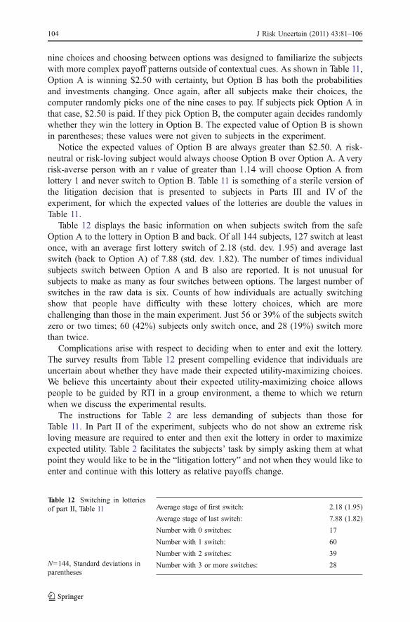
Table 12 displays the basic information on when subjects switch from the safeOption A to the lottery in Option B and back. Of all 144 subjects, 127 switch at leastonce, with an average first lottery switch of 2.18 (std. dev. 1.95) and average lastswitch (back to Option A) of 7.88 (std. dev. 1.82). The number of times individualsubjects switch between Option A and B also are reported. It is not unusual forsubjects to make as many as four switches between options. The largest number ofswitches in the raw data is six. Counts of how individuals are actually switchingshow that people have difficulty with these lottery choices, which are morechallenging than those in the main experiment. Just 56 or 39% of the subjects switchzero or two times; 60 (42%) subjects only switch once, and 28 (19%) switch morethan twice.

Complications arise with respect to deciding when to enter and exit the lottery.The survey results from Table 12 present compelling evidence that individuals areuncertain about whether they have made their expected utility-maximizing choices.We believe this uncertainty about their expected utility-maximizing choice allowspeople to be guided by RTI in a group environment, a theme to which we returnwhen we discuss the experimental results.

The instructions for Table 2 are less demanding of subjects than those forTable 11. In Part II of the experiment, subjects who do not show an extreme riskloving measure are required to enter and then exit the lottery in order to maximizeexpected utility. Table 2 facilitates the subjects’ task by simply asking them at whatpoint they would like to be in the “litigation lottery” and not when they would like toenter and continue with this lottery as relative payoffs change.

Average stage of first switch: 2.18 (1.95)

Average stage of last switch: 7.88 (1.82)

Number with 0 switches: 17

Number with 1 switch: 60

Number with 2 switches: 39

Number with 3 or more switches: 28

Table 12 Switching in lotteriesof part II, Table 11

N=144, Standard deviations inparentheses

104 J Risk Uncertain (2011) 43:81–106

References

Ambrus, A., Greiner, B., & Pathak, P. (2009). Group versus individual decision-making: Is there a shift?Institute for Advanced Study, School of Social Science Economics Working Paper 0091.

Anderson, L. R., & Holt, C. A. (1997). Information cascades in the laboratory. American EconomicReview, 87(5), 847–862.

Anderson, L. R., & Mellor, J. M. (2009). Are risk preferences stable? Comparing an experimental measurewith a validated survey-based measure. Journal of Risk and Uncertainty, 39(2), 137–160.

Aronson, E., Wilson, T. D., & Akert, R. M. (2005). Social psychology (5th ed.). Upper Saddle River:Pearson.

Banerjee, A. V. (1992). A simple model of herd behavior. Quarterly Journal of Economics, 107(3), 797–817.Bikhchandani, S., Hirshleifer, D., & Welch, I. (1992). A theory of fads, fashion, custom, and cultural

change as informational cascades. Journal of Political Economy, 100(5), 992–1026.Bikhchandani, S., Hirshleifer, D., & Welch, I. (1998). Learning from the behavior of others: conformity,

fads, and informational cascades. Journal of Economic Perspectives, 12(3), 151–170.Blinder, A. S., & Morgan, J. (2005). Are two heads better than one? Monetary policy by committee.

Journal of Money, Credit, and Banking, 37(5), 789–811.Brown, R. (1986). Social psychology: The second edition. New York: Free Press.Charness, G., & Gneezy, U. (2007). Strong evidence for gender differences in investment. SSRN Working

Paper.Charness, G., Rigotti, L., & Rustichini, A. (2007). Individual behavior and group membership. American

Economic Review, 97(4), 1340–1352.Cooper, D. J., & Kagel, J. H. (2005). Are two heads better than one? Team versus individual play in

signaling games. American Economic Review, 95(3), 477–509.Daughety, A. F., & Reinganum, J. F. (1999). Stampede to judgment: persuasive influence and herding

behavior by courts. American Law and Economics Review, 1(1), 158–189.Eckel, C. C., & Grossman, P. J. (2008a). Forecasting risk attitudes: an experimental study using actual and

forecast gamble choices. Journal of Economic Behavior and Organization, 68(1), 1–17.Eckel, C. C., & Grossman, P. J. (2008b). Men, women and risk aversion: Experimental results. Working

paper. Forthcoming in C. Plott and V. Smith (eds.), Handbook of Experimental Results. New York:Elsevier.

Fischbacher, U. (2007). z-Tree: Zurich toolbox for ready-made economic experiments. ExperimentalEconomics, 10, 171–178.

Fischhoff, B. (1983). Predicting frames. Journal of Experimental Psychology: Learning, Memory &Cognition, 9, 113–116.

Glaeser, E. L., & Sunstein, C. R. (2009). Extremism and social learning. Journal of Legal Analysis, 1(1),263–324.

Gneezy, U., Niederle, M., & Rustichini, A. (2003). Performance in competitive environments: genderdifferences. Quarterly Journal of Economics, 118(3), 1049–1074.

Goette, L., Huffman, D., & Meier, S. (2006). The impact of group membership on cooperation and normenforcement: evidence using random assignment to real social groups. American Economic Review, 96(2), 212–216.

Guarnaschelli, S., McKelvey, R. D., & Palfrey, T. R. (2000). An experimental study of jury decision rules.American Political Science Review, 94(2), 407–423.

Hargreaves-Heap, S., & Zizzo, D. J. (2009). The value of groups. American Economic Review, 99(1), 295–323.

Healy, A., & Pate, J. (2011). Can teams help to close the gender competition gap? Economic Journal, 121.doi:10.1111/j.1468-0297.2010.02409.x.

Hey, J. D., Morone, A., & Schmidt, U. (2009). Noise and bias in eliciting preferences. Journal of Risk andUncertainty, 39(3), 213–235.

Holt, C. A., & Laury, S. K. (2002). Risk aversion and incentive effects. American Economic Review, 92(5),1644–1655.

Kerr, N. L., MacCoun, R. J., & Kramer, G. P. (1996). Bias in judgment: comparing individuals and groups.Psychological Review, 103(4), 687–719.

Lorenz, J., Rauhut, H., Schweitzer, F., & Helbing, D. (2011). How social influence can undermine thewisdom of crowd effect. Proceedings of the National Academy of Sciences, 108(22), 9020–9025.

Lusk, J. L., & Coble, K. H. (2005). Risk perceptions, risk preference, and acceptance of risky food.American Journal of Agricultural Economics, 87(2), 393–405.

J Risk Uncertain (2011) 43:81–106 105105

http://dx.doi.org/10.1111/j.1468-0297.2010.02409.x

Niederle, M., & Vesterlund, L. (2007). Do women shy away from competition? Do men compete toomuch? Quarterly Journal of Economics, 122(3), 1067–1101.

Rook, L. (2006). An economic psychological approach to herd behavior. Journal of Economic Issues, 40(1), 75–95.

Schkade, D., Sunstein, C. R., & Kahneman, D. (2000). Deliberating about dollars: the severity shift.Columbia Law Review, 100(4), 1139–1175.

Schubert, R., Brown, M., Gysler, M., & Brachinger, H. W. (1999). Financial decision-making: are womenreally more risk-averse? American Economic Review Papers and Proceedings, 89(2), 381–385.

Shupp, R. S., & Williams, A. W. (2008). Risk preference differentials of small groups and individuals.Economic Journal, 118, 258–283.

Sutter, M. (2007). Are teams prone to myopic loss aversion? An experimental study on individual versusteam investment behavior. Economics Letters, 97, 128–132.

Sutter, M. (2009). Individual behavior and group membership: comment. American Economic Review, 99(5), 2247–2257.

Tan, J. H. W., & Bolle, F. (2007). Team competition and the public goods game. Economics Letters, 96(1),133–139.

Wallach, M. A., Kogan, N., & Bem, D. J. (1962). Group influence on individual risk taking. Journal ofAbnormal and Social Psychology, 65(2), 75–86.

106 J Risk Uncertain (2011) 43:81–106

Risky investment decisions: How are individuals influenced ... · Risky investment decisions: How...

Documents

Transcript of Risky investment decisions: How are individuals influenced ... · Risky investment decisions: How...