Can we model the Internet?
47
Can we model the Internet? … and keep it simple Don Towsley Dept. of Computer Science UMass - Amherst large supporting cast: N. Duffield, K. Hollot, W. Gong, Y. Liu, F. Lopresti, V. Misra
Transcript of Can we model the Internet?
Can we model the Internet? … and keep it simple
Don TowsleyDept. of Computer Science
UMass - Amherst
large supporting cast: N. Duffield, K. Hollot,W. Gong, Y. Liu, F. Lopresti, V. Misra
Overview
! introduction! scalable models
" keep it simple!measurement-based models
" keep it simple! summary
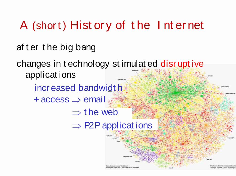
A (short) History of the Internet
after the big bang
changes in technology stimulated disruptiveapplications
increased bandwidth+ access ⇒ email
⇒ the web⇒ P2P applications
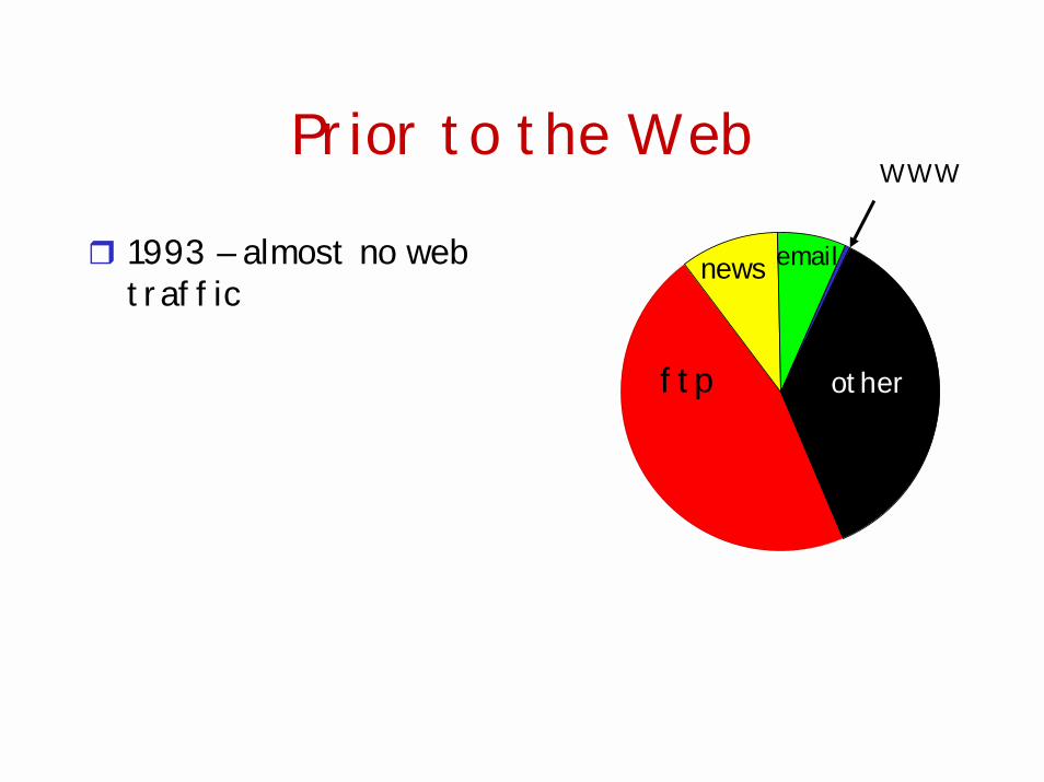
Prior to the WebWWW
ftp
news email
other
! 1993 – almost no web traffic
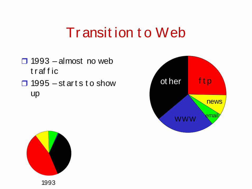
Transition to Web
! 1993 – almost no web traffic
! 1995 – starts to show up
ftp
other
WWW
news
1993
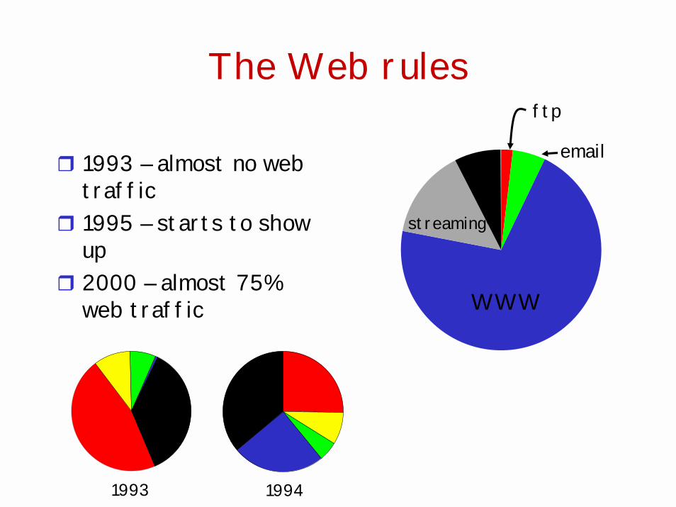
The Web rules
! 1993 – almost no web traffic
! 1995 – starts to show up
! 2000 – almost 75% web traffic
ftp
streaming
emailother
1994
WWW
streaming
1993
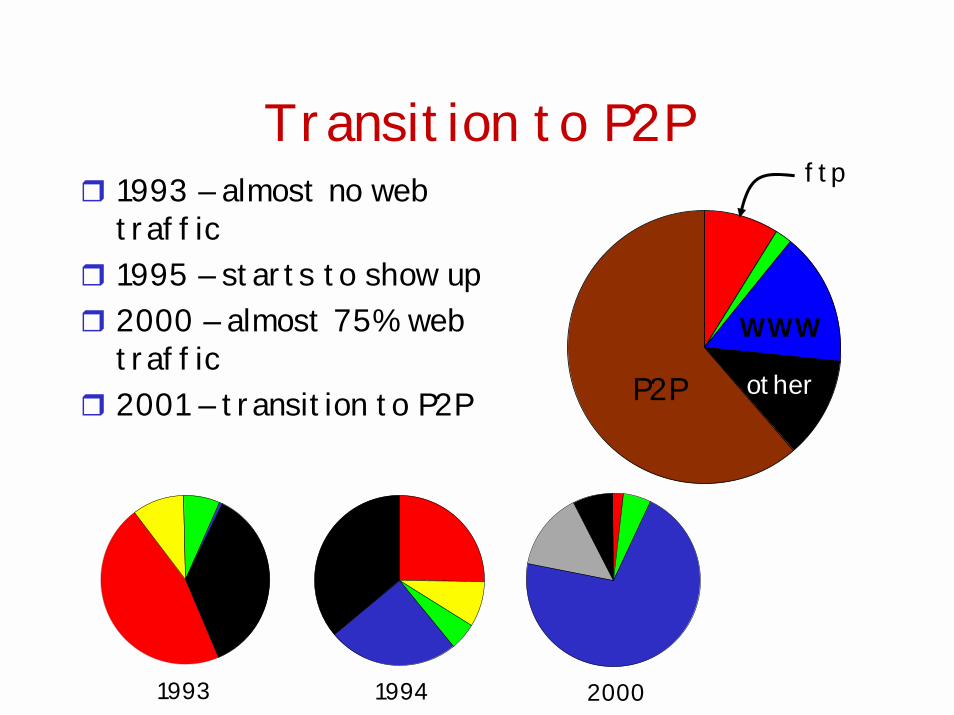
Transition to P2P! 1993 – almost no web
traffic! 1995 – starts to show up! 2000 – almost 75% web
traffic! 2001 – transition to P2P
2000
WWW
P2P other
ftp
1993 1994
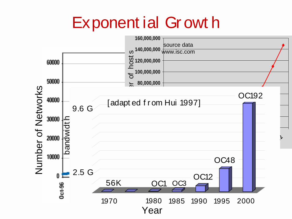
Exponential GrowthN
umbe
r of N
etw
orks
Year
0
20,000,000
40,000,000
60,000,000
80,000,000
100,000,000
120,000,000
140,000,000
160,000,000
1991
1992
1993
1994
1995
1996
1997
1998
1999
2000
2001
2002
source datawww.isc.com
Num
ber
of h
osts
OC192
OC48
OC12OC3OC156K
200019951990198519801970
[adapted from Hui 1997]9.6 G
2.5 G
band
widt
h
how do we model?
understanding?
design?
Invariants
! IP hourglass! predominance of TCP ! mice/elephants
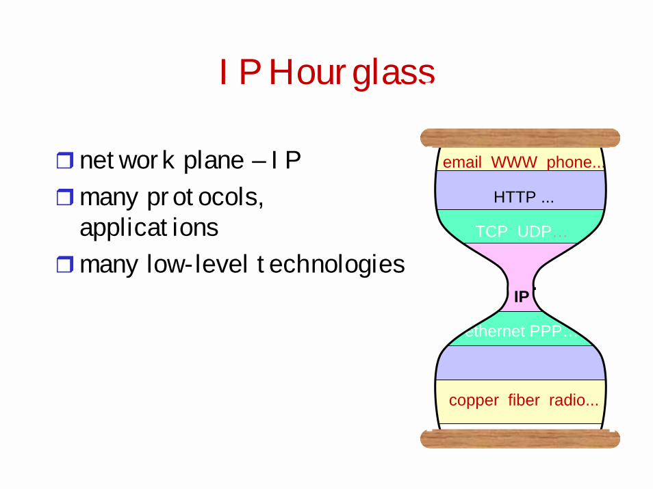
IP Hourglass
! network plane – IP!many protocols,
applications!many low-level technologies
email WWW phone...
HTTP ...
TCP UDP…
IP
ethernet PPP…
copper fiber radio...
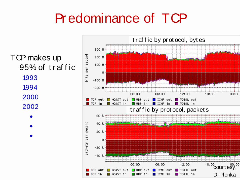
Predominance of TCPtraffic by protocol, bytes
traffic by protocol, packets
courtesy, D. Plonka
TCP makes up 95% of traffic1993199420002002•••
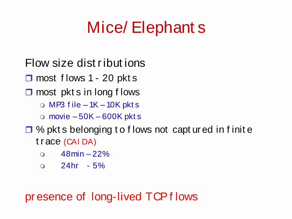
Mice/Elephants
Flow size distributions! most flows 1 - 20 pkts! most pkts in long flows
" MP3 file – 1K – 10K pkts" movie – 50K – 600K pkts
! % pkts belonging to flows not captured in finite trace (CAIDA)" 48min – 22%" 24hr - 5%
presence of long-lived TCP flows
Challenges
Appropriate model for TCP elephants?Level of abstraction?Control strategies?
Models and measurements?
Disclaimer: choice of research problems personal
Themes
! fluids vs packets
! correlation in measurements
! simplicity in modeling
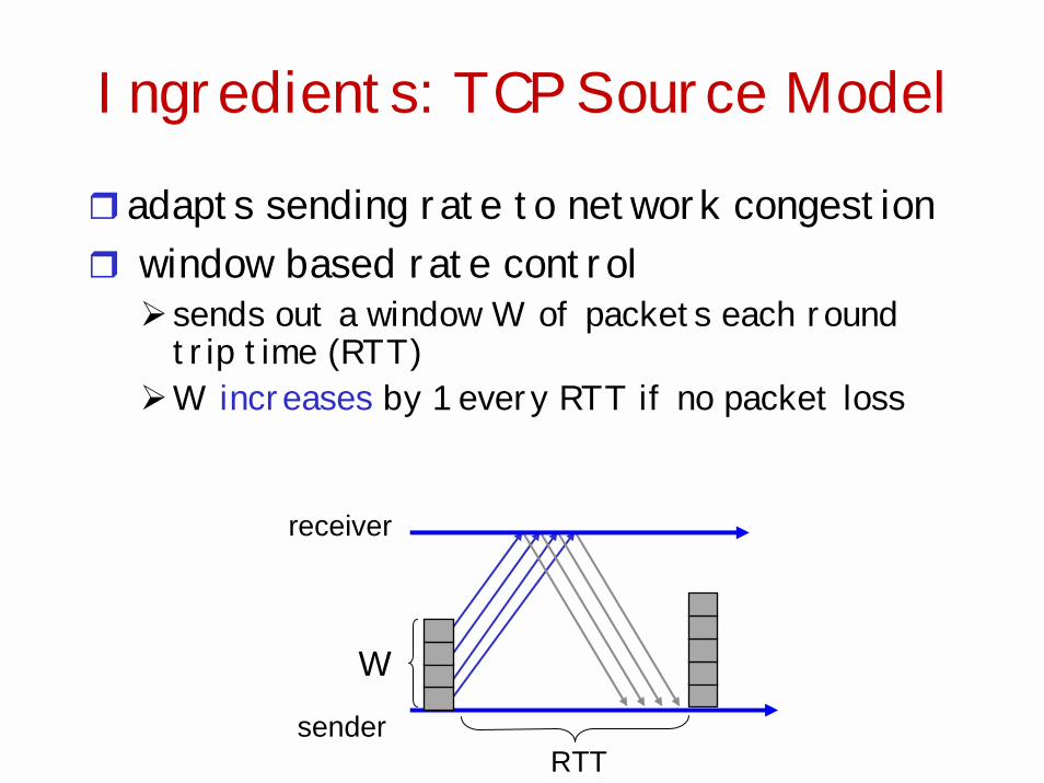
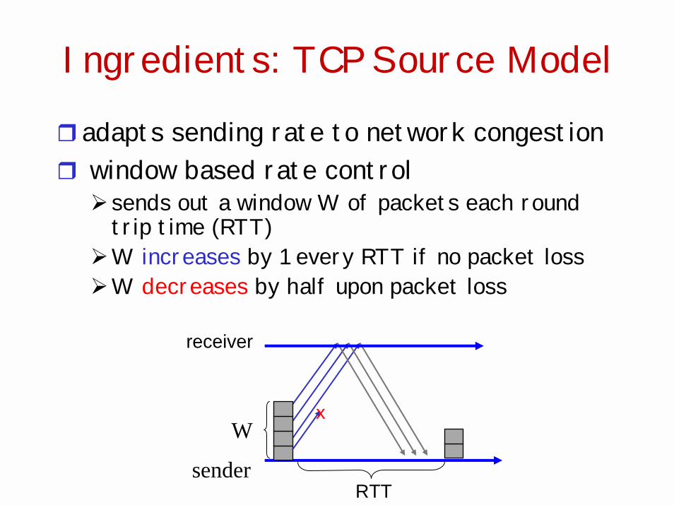
Ingredients: TCP Source Model
! adapts sending rate to network congestion! window based rate control
#sends out a window W of packets each round trip time (RTT)
#W increases by 1 every RTT if no packet loss
sender
receiver
W
RTT
Ingredients: TCP Source Model
! adapts sending rate to network congestion! window based rate control
#sends out a window W of packets each round trip time (RTT)
#W increases by 1 every RTT if no packet loss#W decreases by half upon packet loss
sender
receiver
W
RTT
x
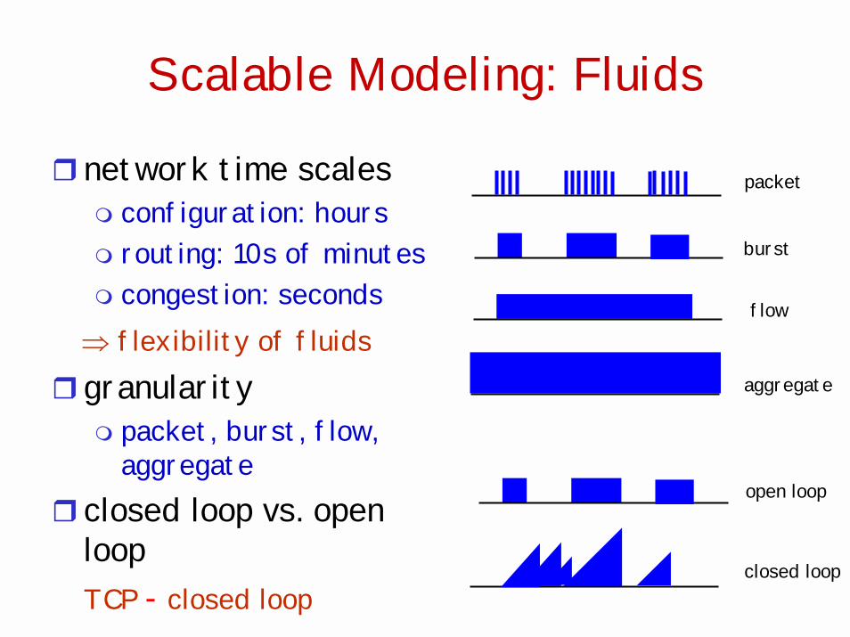
Scalable Modeling: Fluids
! network time scales" configuration: hours" routing: 10s of minutes" congestion: seconds⇒ flexibility of fluids
! granularity" packet, burst, flow,
aggregate! closed loop vs. open
loopTCP - closed loop
packet
burst
flow
aggregate
open loop
closed loop
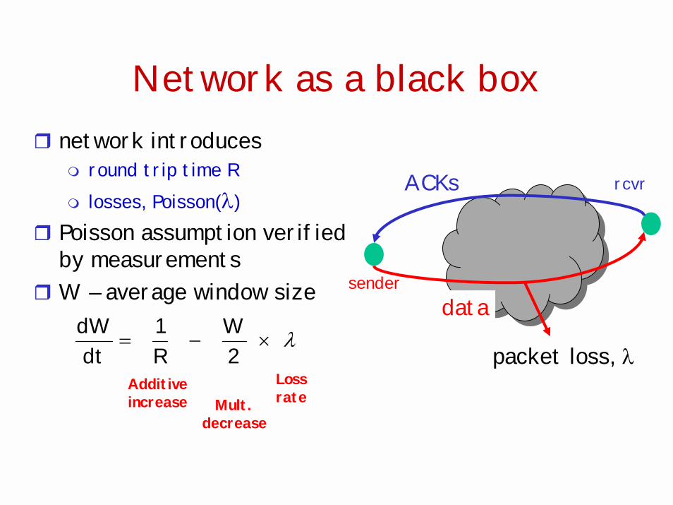
! network introduces" round trip time R" losses, Poisson(λ)
! Poisson assumption verified by measurements
! W – average window size
Network as a black box
data
ACKs
λ×−=2W
R1
dtdW
Additiveincrease
LossrateMult.
decrease
sender
rcvr
packet loss, λ
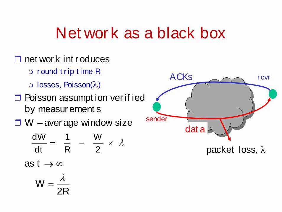
! network introduces" round trip time R" losses, Poisson(λ)
! Poisson assumption verified by measurements
! W – average window size
as t → ∞
Network as a black box
data
ACKs
λ×−=2W
R1
dtdW
sender
R2W λ
=
rcvr
packet loss, λ
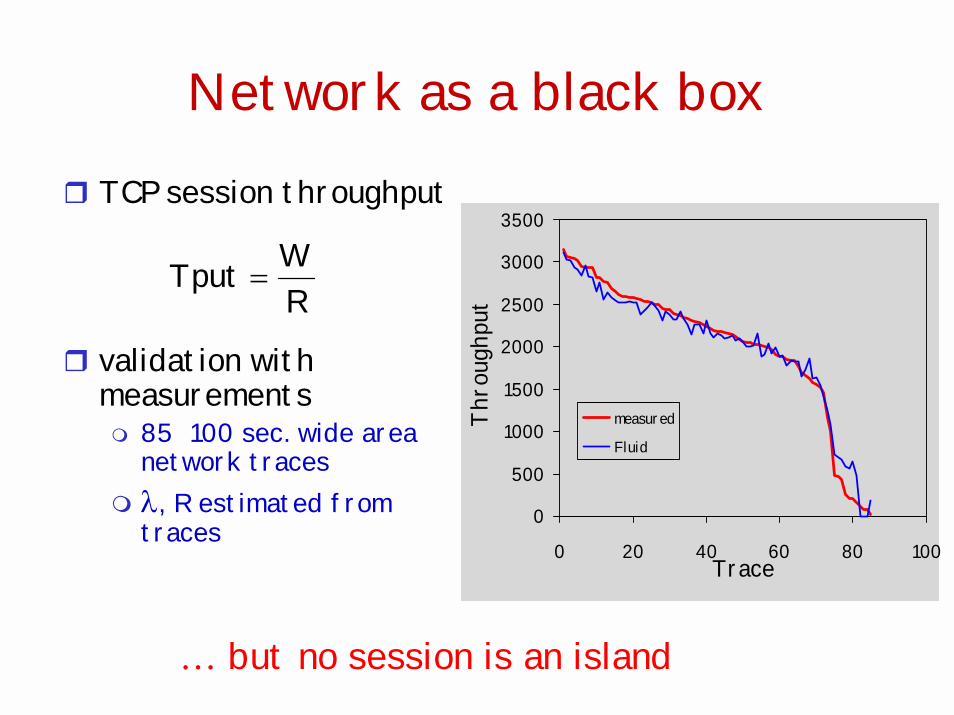
Network as a black box! TCP session throughput
! validation with measurements" 85 100 sec. wide area
network traces" λ, R estimated from
traces 0
500
1000
1500
2000
2500
3000
3500
0 20 40 60 80 100Trace
Thro
ughp
ut
measured
Fluid
RWTput =
… but no session is an island
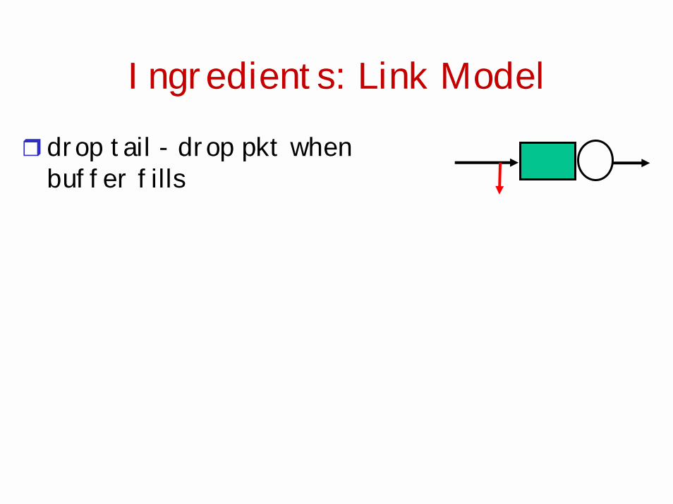
Ingredients: Link Model
!drop tail - drop pkt when buffer fills
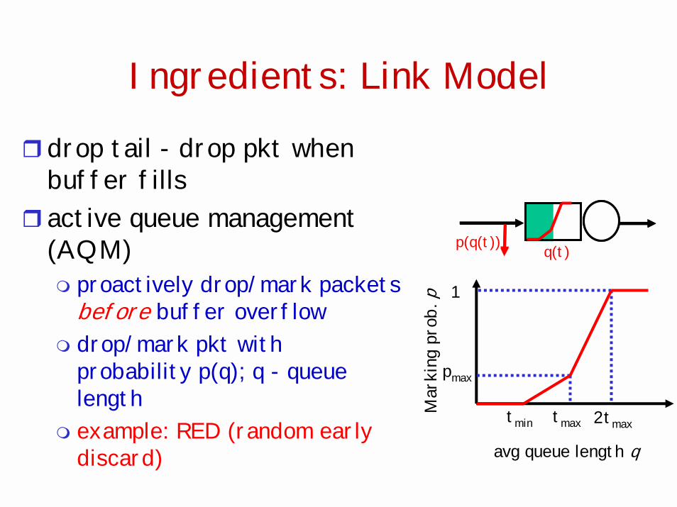
Ingredients: Link Model
!drop tail - drop pkt when buffer fills
! active queue management (AQM)" proactively drop/mark packets
before buffer overflow" drop/mark pkt with
probability p(q); q - queue length
" example: RED (random early discard)
q(t)p(q(t))
tmin tmax
pmax
1
2tmaxM
arki
ng p
rob.
pavg queue length q
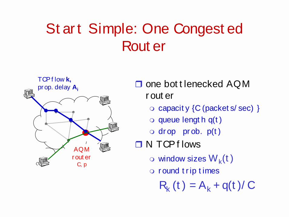
Start Simple: One Congested Router
AQM router
C, p
TCP flow k,prop. delay Ai
! one bottlenecked AQM router" capacity {C (packets/sec) }" queue length q(t)" drop prob. p(t)
! N TCP flows" window sizes Wk(t)" round trip times
Rk (t) = Ak + q(t)/C
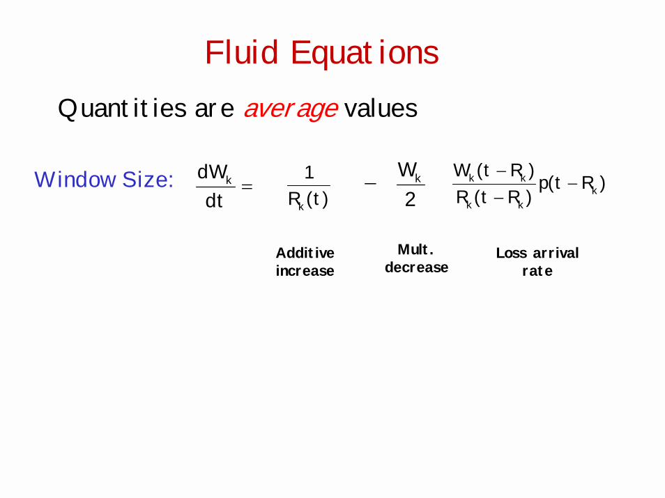
Fluid Equations
Window Size:
Quantities are average values
)t(R1
k=
dtdWk −
2Wk )Rt(p
)Rt(R)Rt(W
kkk
kk −−−
Mult.decrease
Additiveincrease
Loss arrivalrate
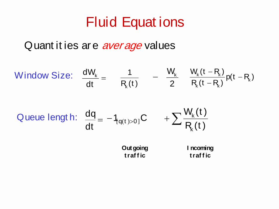
Fluid Equations
Window Size:
Quantities are average values
)t(R1
k=
dtdWk )Rt(p
)Rt(R)Rt(W
kkk
kk −−−−
2Wk
Incomingtraffic
∑+ )t(R)t(W
k
kQueue length: =dtdq
Outgoingtraffic
C1 0tq ])([ >−
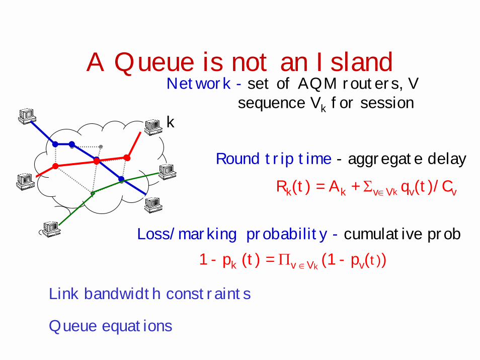
A Queue is not an IslandNetwork - set of AQM routers, V
sequence Vk for sessionk
Loss/marking probability - cumulative prob1 - pk (t) = Πv ∈Vk (1 - pv(t))
Round trip time - aggregate delayRk(t) = Ak + Σv∈Vk qv(t)/Cv
Link bandwidth constraints
Queue equations
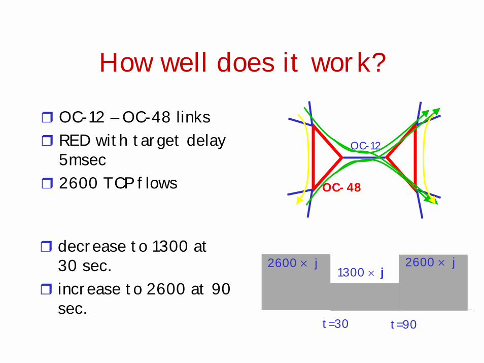
How well does it work?
OC-48
OC-12
! OC-12 – OC-48 links! RED with target delay
5msec! 2600 TCP flows
! decrease to 1300 at 30 sec.
! increase to 2600 at 90 sec.
t=30 t=90
2600 × j 2600 × j1300 × j
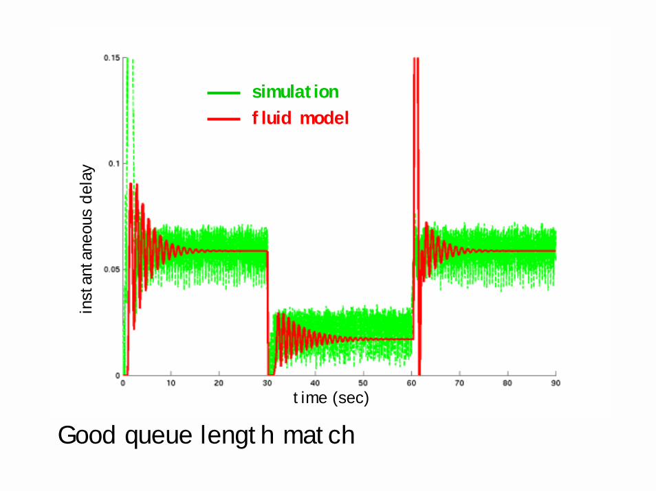
Good queue length match
inst
anta
neou
s de
lay
time (sec)
simulationfluid model
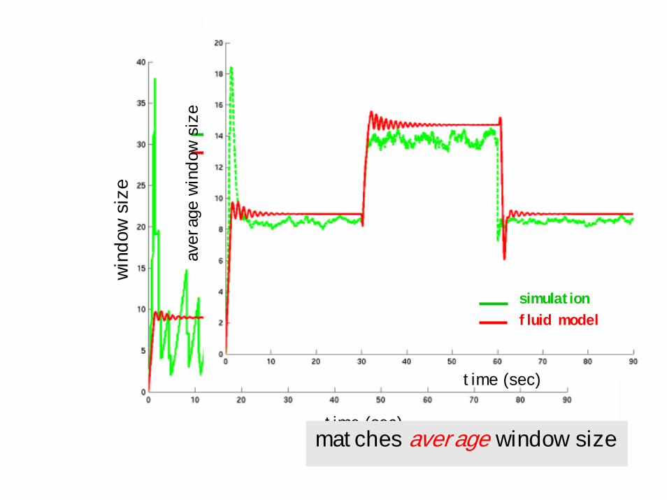
time (sec)
wind
ow s
ize
matches average window size
simulationfluid model
time (sec)
aver
age
wind
ow s
ize
simulationfluid model
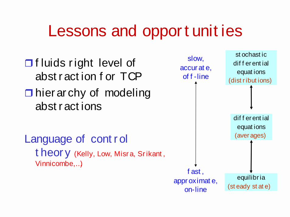
Lessons and opportunitiesstochastic
differentialequations
(distributions)
slow,accurate,off-line
fast,approximate,
on-line
! fluids right level of abstraction for TCP
!hierarchy of modeling abstractions
Language of control theory (Kelly, Low, Misra, Srikant, Vinnicombe,…)
differentialequations
(averages)
equilibria(steady state)
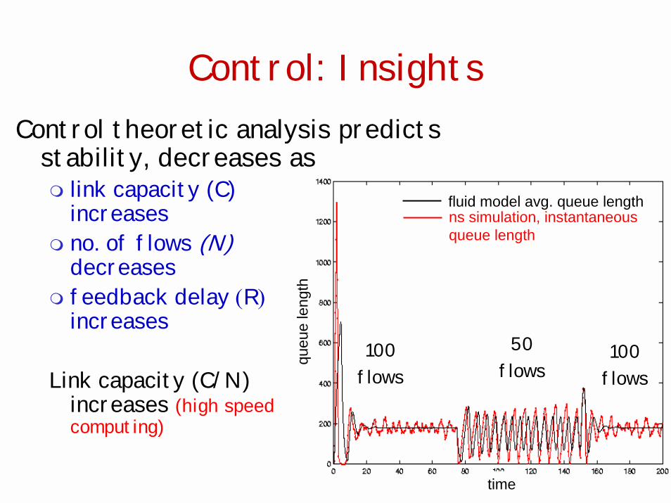
Control: Insights
100flows
100flows
50flows
ns simulation, instantaneous queue length
fluid model avg. queue length
time
queu
e le
ngth
Control theoretic analysis predicts stability, decreases as" link capacity (C)
increases" no. of flows (N)
decreases" feedback delay (R)
increases
Link capacity (C/N) increases (high speed computing)
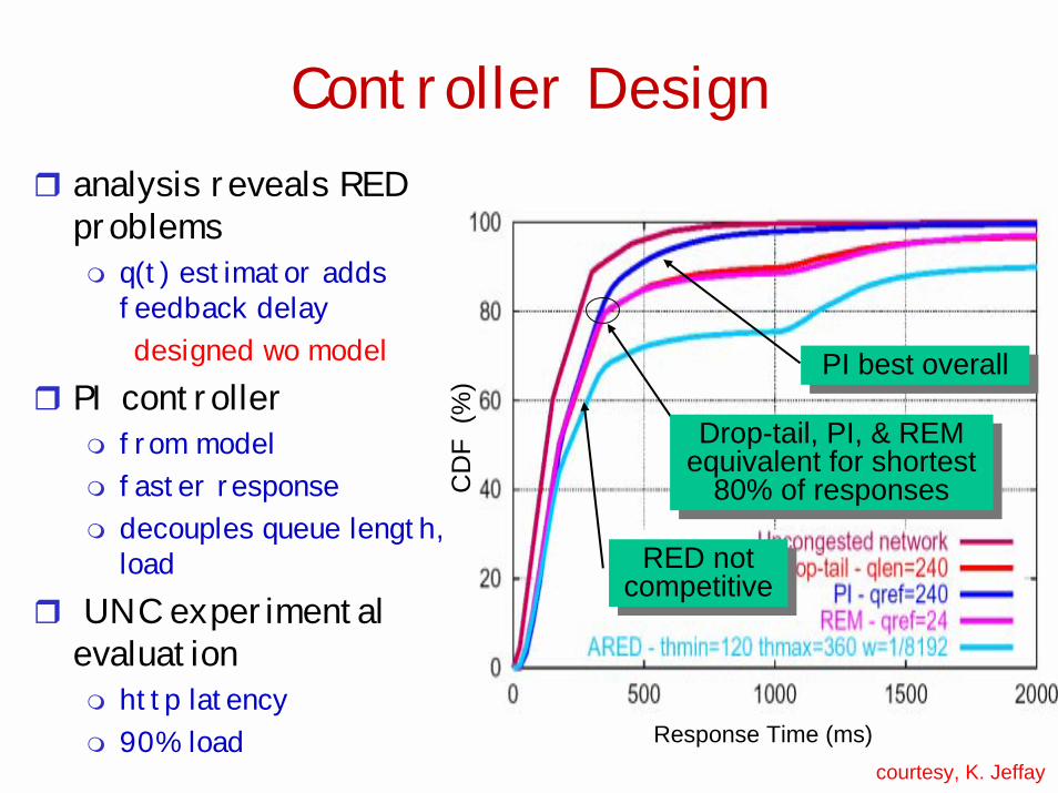
Controller Design
CD
F (%
)
Response Time (ms)
Drop-tail, PI, & REM equivalent for shortest
80% of responses
Drop-tail, PI, & REM equivalent for shortest
80% of responses
PI best overallPI best overall
RED not competitiveRED not
competitive
! analysis reveals RED problems" q(t) estimator adds
feedback delaydesigned wo model
! PI controller" from model" faster response" decouples queue length,
load! UNC experimental
evaluation" http latency" 90% load
courtesy, K. Jeffay
models and measurements
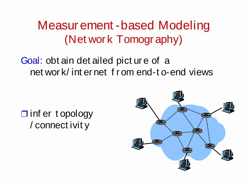
Measurement-based Modeling (Network Tomography)
Goal: obtain detailed picture of a network/internet from end-to-end views
! infer topology /connectivity
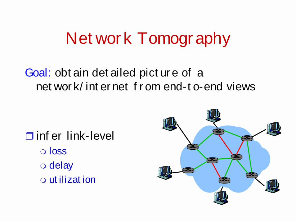
Network Tomography
Goal: obtain detailed picture of a network/internet from end-to-end views
! infer link-level" loss" delay" utilization
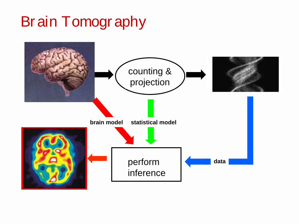
Brain Tomography
unknownobject
counting &projection
Maximumlikelihood estimate
performinference
data
statistical modelbrain model
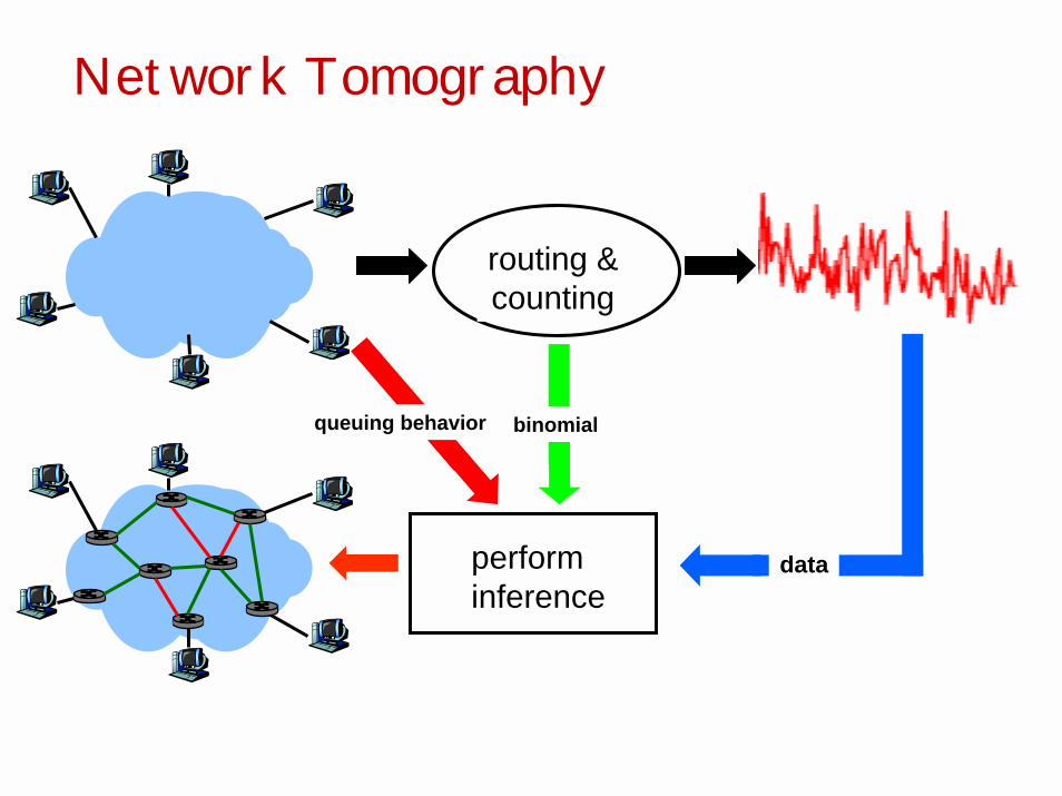
Network Tomography
routing &counting
data
queuing behavior binomial
performinference
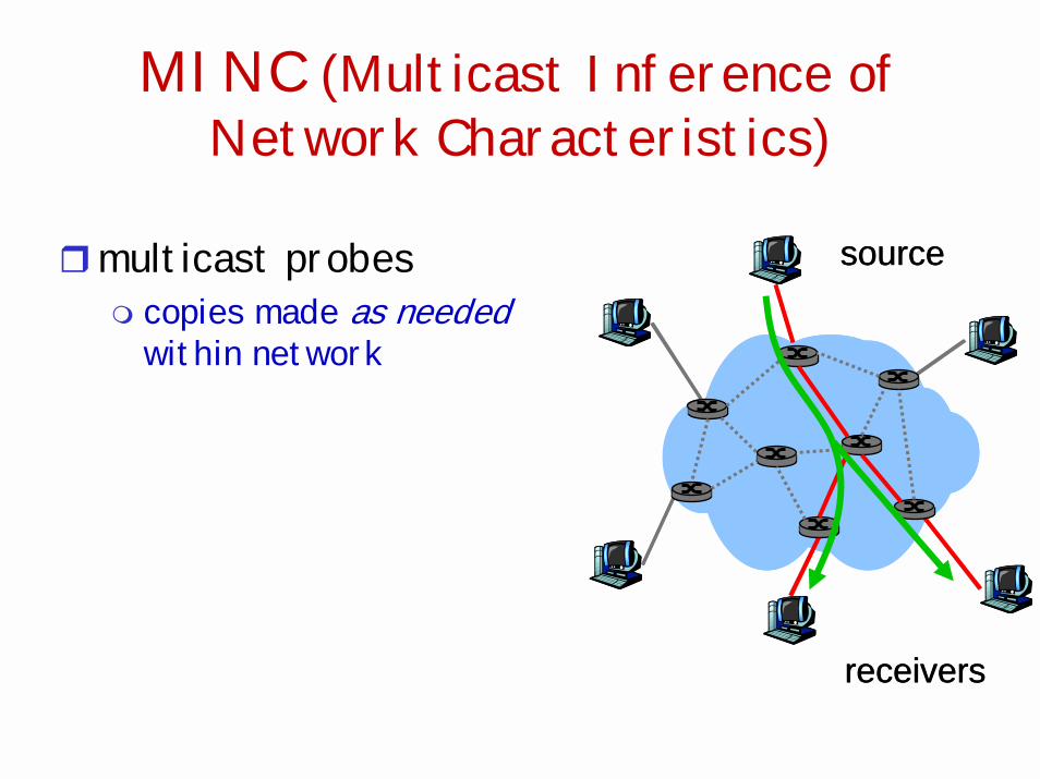
MINC (Multicast Inference of Network Characteristics)
!multicast probes" copies made as needed
within network
source
receivers
source
receivers
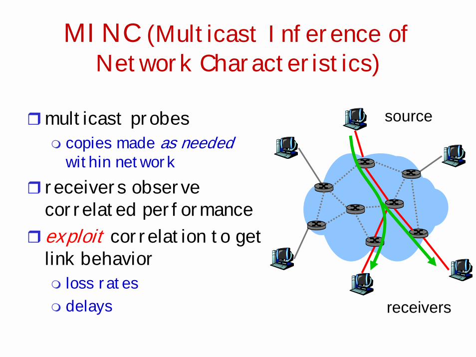
MINC (Multicast Inference of Network Characteristics)
!multicast probes" copies made as needed
within network! receivers observe
correlated performance! exploit correlation to get
link behavior" loss rates" delays
source
receivers
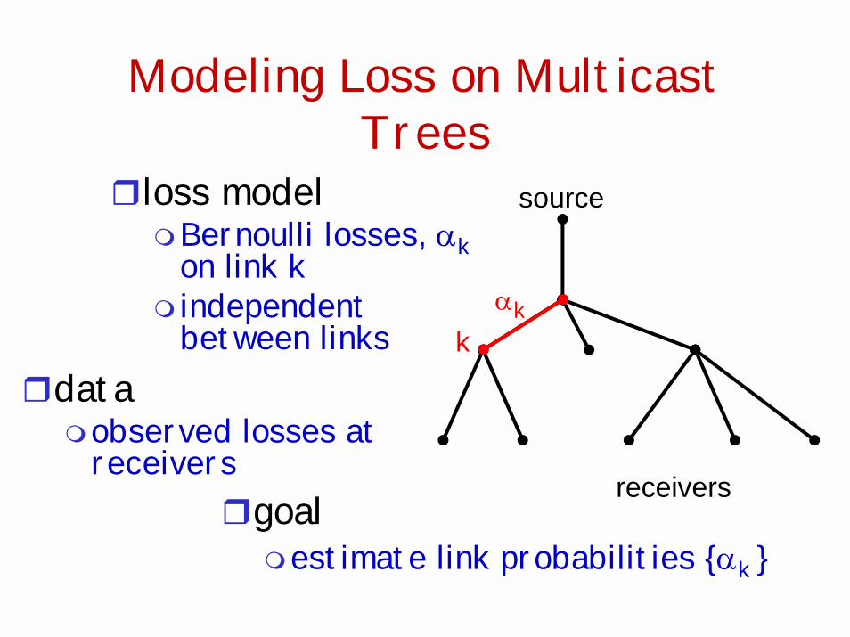
Modeling Loss on Multicast Trees
source
receivers
kαk
!loss model"Bernoulli losses, αk
on link k " independent
between links!data
"observed losses at receivers
!goal "estimate link probabilities {αk }
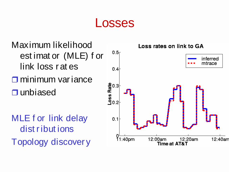
LossesMaximum likelihood
estimator (MLE) for link loss rates
!minimum variance! unbiased
MLE for link delay distributions
Topology discovery
Lessons and Opportunities
! correlation powerful tool!" multicast, packet pairs, sandwiches, stripes
!measurement-based modeling rich, wide open research area" edge-based" router-based “monitor in the middle”" hybrid approaches" application-based
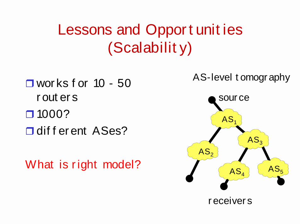
Lessons and Opportunities (Scalability)
source
receivers
AS-level tomography
AS1
AS2
AS3
AS4AS5
!works for 10 - 50 routers
! 1000? !different ASes?
What is right model?
Other modeling successes
! open loop traffic (Mitra, …)
! network calculus (Cruz, Chang, LeBoudec, …)
! security (Zou, …)
" malware as fluids
Summary
! invariants permit reasoned approach to modeling
! fluids allow scalable modeling
need to go beyond data plane to control plane
! correlation key to measurement-based modeling" how to introduce, quantify, control?
still missing - a measurement science
The end
Thanks!
Slides (will be) available athttp://gaia.cs.umass.edu/towsley/dtc03.pdf