IN DEGREE PROJECT ELECTRICAL ENGINEERING,SECOND CYCLE, 30 CREDITS

, STOCKHOLM SWEDEN 2017

Calibration of Vibration sensors - Evaluation and Effectivization

VLADIMIR CHEVATCO

KTH ROYAL INSTITUTE OF TECHNOLOGYSCHOOL OF ELECTRICAL ENGINEERING

Calibration of Vibration sensors – Evaluation and

Effectivization

Vladimir Chevatco

Abstract

In this thesis, the calibration process of a geophone based vibration sensor istreated and optimised. The purpose of calibration is to estimate the physicalparameters of the system in the form of gain, damping and eigenfrequency.The geophone is calibrated on a shaker, and this thesis deals with the choiceof input signals and parameter estimation methods. Three different inputsignals are evaluated, and a new calibration process based on a multi-toneexcitation coupled with system identification methods for parameter estima-tion is proposed.

Sammanfattning

I detta examensarbete studeras kalibreringsprocessen for ett geofon-baseratmatinstrument. Malet med kalibreringen ar att skatta matinstumentets egen-skaper i form av egenfrekvens, dampning och forstarkning. Instrumentet ka-libreras pa ett skakbord och valet av insignal till skakbordet samt parame-terskattningsmetoden behandlas. Tre olika insignaler testas och en ny ka-libreringsprocess som anvander multiton-insignaler och systemidentifieringfor parameterskattning presenteras.

Contents

1 Introduction 31.1 Background . . . . . . . . . . . . . . . . . . . . . . . . . . . . 31.2 Problem formulation . . . . . . . . . . . . . . . . . . . . . . . 41.3 Outline . . . . . . . . . . . . . . . . . . . . . . . . . . . . . . . 5

2 Theory 62.1 System identification . . . . . . . . . . . . . . . . . . . . . . . 62.2 Experimental design . . . . . . . . . . . . . . . . . . . . . . . 8

2.2.1 Swept-sine . . . . . . . . . . . . . . . . . . . . . . . . . 92.2.2 Multitones . . . . . . . . . . . . . . . . . . . . . . . . . 112.2.3 Optimal input signals . . . . . . . . . . . . . . . . . . . 12

3 Evaluation of current method 143.1 Background . . . . . . . . . . . . . . . . . . . . . . . . . . . . 143.2 Measurement hardware . . . . . . . . . . . . . . . . . . . . . . 163.3 Process . . . . . . . . . . . . . . . . . . . . . . . . . . . . . . . 173.4 Accuracy constraints . . . . . . . . . . . . . . . . . . . . . . . 19

4 Test pulse overview 22

5 Method 255.1 Modification of current method. . . . . . . . . . . . . . . . . . 255.2 System identification approach . . . . . . . . . . . . . . . . . . 28

5.2.1 Modelling . . . . . . . . . . . . . . . . . . . . . . . . . 285.2.2 Input signal selection . . . . . . . . . . . . . . . . . . . 295.2.3 Estimation and verification . . . . . . . . . . . . . . . . 33

5.3 On gain estimation . . . . . . . . . . . . . . . . . . . . . . . . 36

6 Discussion 36

7 Future work 38

8 Bibliography 38

2

1. Introduction

Vibration monitoring is an important part of engineering, with many ap-plications. It can be used for evaluating comfort in vehicles, monitoring thestatus of a working device, or to ensure structures are not subjected to overlyhigh loads, just to name a few examples. There are many ways to measurevibrations, both with regards to the measured quantity (displacement, ve-locity, or acceleration), and the intended application area of the results. Inthis thesis we will focus on the use of a geophone, which measures vibrationvelocity, as applied to structural monitoring at construction sites. This ismore an just an engineering curiosity, rather there are legal standards whichrequire this measurement to be conducted in order to ensure the safety ofthe operation and not damage nearby structures. Therefore it is of highestimportance that the measurement device used is calibrated correctly and canmeasure according to the relevant standard. This thesis concerns itself withthe application of system identification methods to optimise the calibrationprocess of the vibration sensors.

1.1. Background

The vibration measurement device uses a geophone sensor element, and inorder to correctly recover the amplitudes of vibration, calibration is needed.A geophone is a high sensitivity device used traditionally to measure groundmovement, consisting of a magnetic mass moving inside a wire coil as shownin Figure 1. From this figure it can be seen that the geophone is an electrome-chanical system, expressed as a mass-spring-damper system coupled with anLR-circuit. The movement of the magnetic mass inside the coil induces avoltage which is proportional to the velocity of the motion. By sending acurrent through the coil it is also possible to exert a force on the magnet,displacing it. This functionality is called a ”test pulse” in the context of thisthesis, and will be explored in more detail later. Under normal conditionsthe electrical system should interfere as little as possible with the movementof the magnet. For the purposes of this thesis, the geophone is mathemati-cally modelled as a second order transfer function from vibration velocity tovoltage expressed as (1).

G(s) = Ks2

s2 + 2ζω0s+ ω20

(1)

3

Figure 1: A geophone and its working principle.

This transfer function is also known as the sensitivity of the geophone withunits volt per m/s. For calibration purposes, the magnitude of this transferfunction needs to be known over a wide frequency range. This necessitatesa good estimation of the parameters K (Gain), ζ (damping) and ω0 (eigen-frequency).

1.2. Problem formulation

This thesis focuses on finding fast and accurate methods to estimate thegain, eigenfrequency and damping of a geophone, using system identificationtechniques.The expected results from this thesis will answer the following questions:

1. How sensitive is the current method to estimation errors in the param-eters of interest?

2. How accurate is the current method?

3. Is it possible to speed up the calibration process by utilizing systemidentification methods?

4. Are the results accurate enough?

5. Can the test-pulse functionality be of use?

Finally, if the answer to questions 3 & 4 are in the affirmative, a new cali-bration procedure optimised for speed will be specified and implemented.

4

1.3. Outline

In order to answer the questions posed, an outline of the solution is presentedbelow. First, a sensitivity analysis of the system is conducted, based both ontheoretical analysis, and the current calibration method, in order to establishthe bounds and requirements on the accuracy of the estimation.Then, two different approaches are tested in order to speed up the calibrationprocess:

1. A modification of the current calibration process.

2. System identification based approach using persistent and periodic in-puts (multi-sine, noise, etc).

Finally the accuracy and performance of the different methods are discussedand compared.In the following Chapter, an overview of the theory of system identificationmethods is given, focusing on experimental design and system identificationin practice. Chapter 3 covers the evaluation of the current method withregard to accuracy and sensitivity. Chapter 4 covers the self-test functionalityof the measurement device. The two different approaches are presented indetail in Chapter 5, and a discussion follows in Chapter 6.

5

2. Theory

2.1. System identification

System identification and estimation techniques are a class of statisticalmethods used to identify process models and find optimal values for modelparameters from observed data, which tends to be incomplete, noise-affectedor otherwise imperfect. Such a broad definition means that these methodscan be applied to everything from financial data to biochemical processes.In the field of vehicle engineering perhaps the most relevant example wouldbe the recent developments in autonomous vehicles and intelligent transportsystem (ITS). Such systems take a large amount of data available via varioussensors, GPS signals, mathematical models and so on, and use this data tomake an estimate of a quantity of interest(position, speed, etc.) better thaneach individual data source could. Another application of system identifi-cation methods that gained popularity with the ever-increasing computingpower available is identification for control, where a plant model is estimatedin real time and a control system is synthesised to provide the best per-formance possible. This is also known as adaptive control and is also veryimportant to vehicles. A thorough treatment of this topic is given in [3] and[5] so a shorter overview of the most relevant subjects will be given here. Aninput-output relation in an LTI system can be represented using the followingmodel:

y(t) = G(q, θ)u(t) +H(q, θ)e(t) (2)

where q can be the time-shift operator in the case of a discrete time system,the derivative operator for continuous-time systems, or whatever is mostappropriate. The principle remains the same. G is the transfer functionfrom the input u(t) to the output y(t) and H is the transfer function fromthe disturbance e(t) to the output. Generally, G and H are modelled asrational polynomials in q, with unknown parameter vector θ:

G(q, θ) =b0 + b1q

−1 + ...+ bmq−m

1 + a1q−1 + ...+ anq−n

H(q, θ) =1 + c1q

−1 + ...+ ckq−k

1 + d1q−1 + ...+ dlq−l

The parameter vector θ contains the polynomial coefficients:

θ =[a1 . . . an b1 . . . bm c1 . . . ck d1 . . . dl

]T6

Now the task of identifying the system can be thought of as identifying themodel order (the order of the polynomials in the transfer function) and thecoefficients so that (2) fits the measured data best.One popular choice of ”best fit” is to choose θ such that the difference betweenthe predicted output of the system and the measured one is minimized. Ifr(t, θ) = y(t, θ) − y(t, θ) is the prediction error and the predictor y(t, θ) isgiven by

y(t, θ) = H−1Gu(t) + (1−H−1)y(t) (3)

then the problem can be set up as an optimization problem with the optimalsolution given by:

θ∗ = argminθ1

N

N∑t=1

r(t, θ)T r(t, θ) (4)

with N being the number of samples in the signal. This is called the Predic-tion Error (PE) method, and is widely used.Commonly the transfer function is studied in the frequency domain, and suchis the case with this thesis. Due to the way the current system is built, thereis no synchronization between the input and output channels which can alsobe of different sample rates. One approach would be to try and estimatethe delays between the data sets. A more simple approach is to study thesystem in the frequency domain. In the frequency domain representation,prediction is not very meaningful, so a modification to (3) and (4) is needed.The frequency domain representation of (2) can be written as

Y (ω) = G(ω, θ)U(ω) +H(ω, θ)E(ω) (5)

Where Y , U , and E are the Fourier transforms of the output, input, andnoise, respectively. In the same way, the minimizer in the frequency domainis given as

θ∗ = argminθ1

N

∥∥∥∥Y (ω)

U(ω)−G(θ, ω)

∥∥∥∥2 ‖U(ω)‖2

‖H(θ, ω)‖2(6)

for N frequencies. This can be seen as choosing θ such that the differencebetween the measured transfer function and the model is minimized, usinga weighing filter that favors frequencies where the input has more power orthe noise has less power. It is important to note that there is no unique way

7

to choose a cost function to minimize as any reasonable choice leads to anestimator. However, different choices do lead to different behaviors of theestimator with regards to efficiency, correctness, etc. The form of (6) impliesseveral things:

1. It is important to measure the empirical frequency response Y (ω)U(ω)

well,as it is the base of the fit.

2. More data (frequency points) leads to better estimates due to the 1/Nfactor in (6).

3. It is important that the input signal excites the system well and pro-duces good response with low noise (good SNR) .

4. If the noise model H is trivial (i.e H = 1) the weight in (6) is propor-tional to the power of the input signal.

How to measure the frequency response function (FRF) well and how tochoose the correct input signal for the task is discussed next.

2.2. Experimental design

The purpose of an identification experiment is to extract information aboutthe system of interest. In purely autoregressive systems, that is, systems inwhich the future output depends solely on previous outputs, experiment de-sign comes down to how to measure the output. Systems with a controllableinput provide much more flexibility and choice in the design of the identifica-tion experiment. With regards to measurement settings, three main factorsaffect the results:

1. Sampling frequency Fs. Determines upper bound on measurementbandwidth as given by the Shannon/Nyquist theorem.

2. Measurement duration. Determines frequency resolution as df = 1/T .

3. Quantization bit-depth. Determines minimum amplitude resolution inthe ADC.

The best choice of excitation signal is not a simple matter, as it dependson the system itself, and can in general be of any form. In practice, somelimitations apply.

1. Input signal must have a finite amplitude.

2. Input signal must excite all the interesting features of the system.

3. Periodic inputs have some advantages over non periodic ones.

8

In addition, some constraints resulting from the used measurement equip-ment and purpose with the calibration, narrow down the selection.

1. The input to the system is generated using a shaker, so impulse exci-tations are not possible.

2. The purpose of the new system is to save time. Because noise signalsrequire windowing and averaging (and thus longer measurement times),using deterministic, periodic signals is preferred.

There are some standard choices of input signal type, each with their ownadvantages and disadvantages. As these are covered in detail in for example[3] and [5], only the input signals used during the course of the thesis arecovered in detail.

2.2.1. Swept-sine

Figure 2: Swept sine

Swept sine excitation uses a sine wave with a time varying frequency inorder to excite the system. The energy per frequency is then proportional tothe time spent at that frequency. The signal in the time domain is similarto Figure 2. A sweep that varies linearly from ω1 to ω2 in time T can bedescribed mathematically as:

slin(t) = sin(φ(t)) = sin(ω1t+ω2 − ω1

T· t

2

2) (7)

9

Such a signal has a equal energy between the swept frequencies, much likewhite noise, but has the advantage of being deterministic. An exponentiallytime varying sweep can be described as:

sexp(t) = sin(φ(t)) = sin(K · (etL − 1)) (8)

where

K =T · ω1

ln(ω2

ω1)

(9)

L =T

ln(ω2

ω1)

(10)

Such a signal has a 1/f power spectrum, much like pink noise. The signal inthe frequency domain is shown in Figure 3. Since the signal is deterministic

Figure 3: Exponential sweep.

each realisation of the signal is identical except for noise. If the signal alsostarts and ends at 0, no windowing is needed. A good FRF can be thereforeestimated from just one sweep, if noise is not a major issue. In additionthe crest factor for this signal is identical to that of a sine wave. This al-lows for quick and reliable measurements, much faster than the stepped-sineapproach.The major disadvantage of these signals is that the time domain constructionlike in (7) and (8) leads to some artifacts in the frequency domain in theform of very obtrusive ripples at the edge of the passband, like can be seen

10

in figure 3 at around 20 and 1000 Hz. A solution is to instead construct it inthe frequency domain as described in [4]. The resulting signal has drasticallyreduced ripple (Figure 4), even if it cannot be eliminated completely.

(a) Modified sweep in time domain. (b) modified sweep in frequency domain.

Figure 4: Reduced ripple sweep.

2.2.2. Multitones

Multitones in this context refers to a sum-of-sinusoids signals. While tech-nically any signal can be considered a sum-of-sines signal, we refer here toa signal with discrete, user selected frequencies. In general the signal canbe described mathematically as s =

∑mk=1Aksin(ωkt + φk) and a time and

frequency representation of a signal with 32 frequencies from 1 to 32 Hz isshown in Figure 5.The major advantages with these types of signals is that the spectrum canbe shaped easily. Energy in the signal is concentrated to the chosen frequen-cies and is not ”wasted” elsewhere, leading to better SNR. In addition, thesignal is periodic so no windowing is needed if the record time is chosen cor-rectly. The disadvantage is that the signal has poor crest factor in the naiveimplementation(φk=0), and generally the phases φk of the components mustbe randomized to achieve a better crest factor. This adds a random elementto this signal. The frequency content also must be chosen over a specific gridto guarantee the signal is periodic in the time window.

11

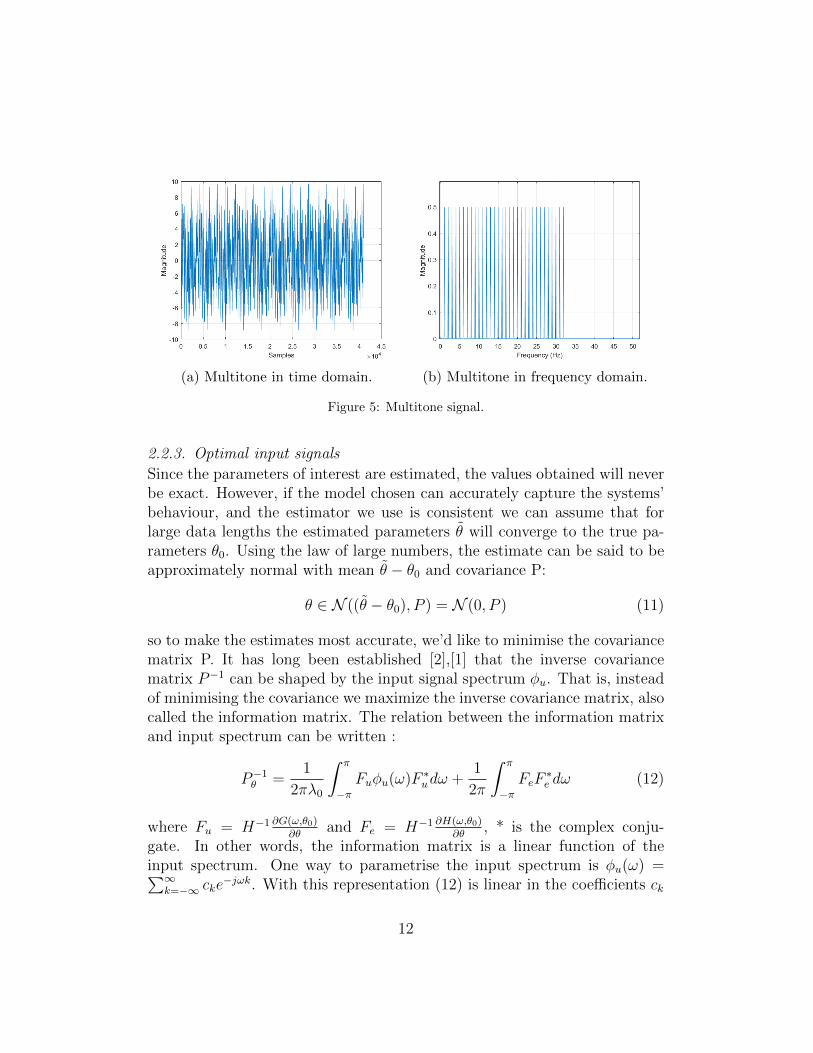
(a) Multitone in time domain. (b) Multitone in frequency domain.

Figure 5: Multitone signal.

2.2.3. Optimal input signals

Since the parameters of interest are estimated, the values obtained will neverbe exact. However, if the model chosen can accurately capture the systems’behaviour, and the estimator we use is consistent we can assume that forlarge data lengths the estimated parameters θ will converge to the true pa-rameters θ0. Using the law of large numbers, the estimate can be said to beapproximately normal with mean θ − θ0 and covariance P:

θ ∈ N ((θ − θ0), P ) = N (0, P ) (11)

so to make the estimates most accurate, we’d like to minimise the covariancematrix P. It has long been established [2],[1] that the inverse covariancematrix P−1 can be shaped by the input signal spectrum φu. That is, insteadof minimising the covariance we maximize the inverse covariance matrix, alsocalled the information matrix. The relation between the information matrixand input spectrum can be written :

P−1θ =1

2πλ0

∫ π

−πFuφu(ω)F ∗udω +

1

2π

∫ π

−πFeF

∗e dω (12)

where Fu = H−1 ∂G(ω,θ0)∂θ

and Fe = H−1 ∂H(ω,θ0)∂θ

, * is the complex conju-gate. In other words, the information matrix is a linear function of theinput spectrum. One way to parametrise the input spectrum is φu(ω) =∑∞

k=−∞ cke−jωk. With this representation (12) is linear in the coefficients ck

12

which can then be solved for. This approach however is not feasible sincethere are infinitely many coefficients ck. To make the problem feasible aso-called finite spectrum parametrization can be used [1]. In this approach,the series expansion is truncated after M terms, and the real positive part isused:

φu(ω) =M∑k=0

cke−jωk + conj(

M∑k=0

cke−jωk)

This approach, combined with constraints on the input signal, can produce anexcitation spectrum which yields the most accurate estimates. Two things areworth noting however. First is that this approach produces a technically sub-optimal solution due to the truncation of the spectrum expansion. Second,this only provides a frequency domain description of the signal. The timedomain realisation of this spectrum is a different issue, as there are manysignals with identical spectrum. This optimal approach was considered forthis thesis, but ended up not being used, due to the fact that a satisfactoryresult was obtained using swept and multi-sine signals. Nevertheless, froma theoretical point of view optimal signal generation can be interesting forfuture work.

13

3. Evaluation of current method

3.1. Background

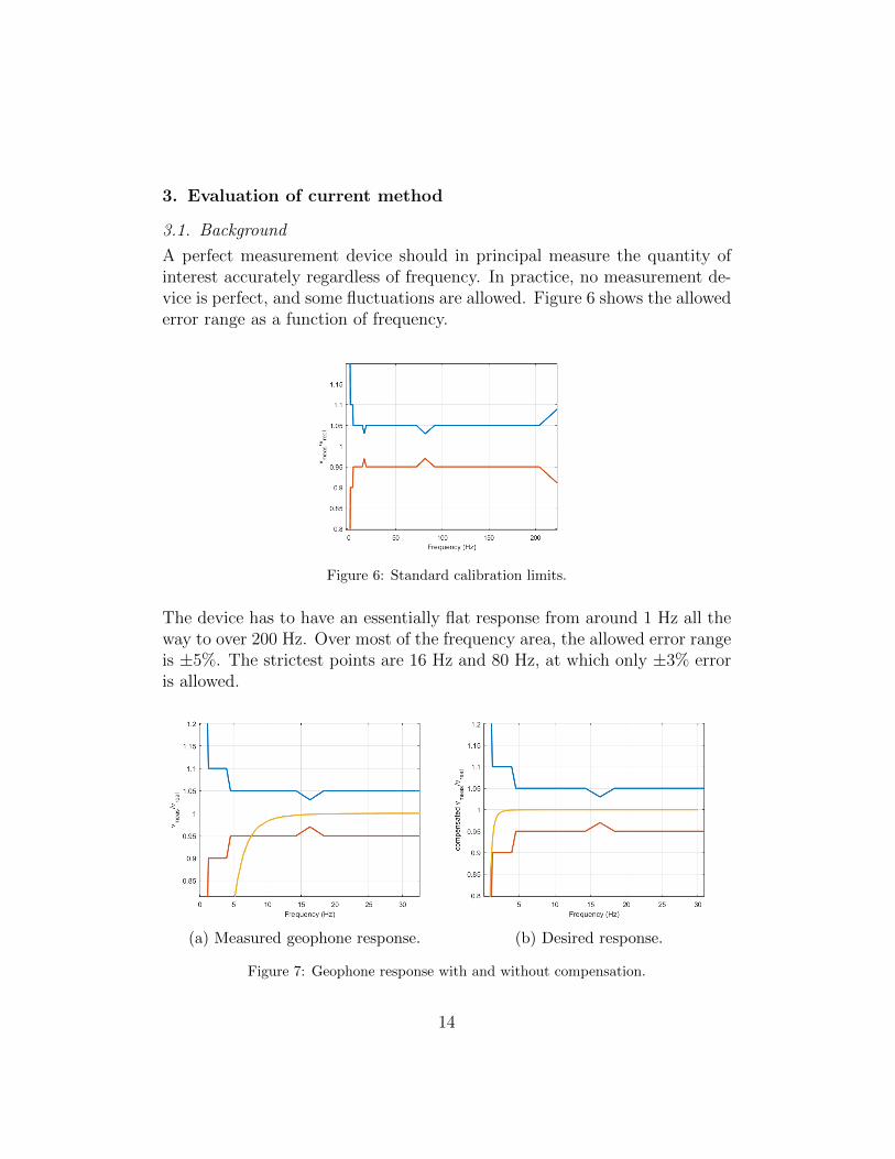
A perfect measurement device should in principal measure the quantity ofinterest accurately regardless of frequency. In practice, no measurement de-vice is perfect, and some fluctuations are allowed. Figure 6 shows the allowederror range as a function of frequency.

Figure 6: Standard calibration limits.

The device has to have an essentially flat response from around 1 Hz all theway to over 200 Hz. Over most of the frequency area, the allowed error rangeis ±5%. The strictest points are 16 Hz and 80 Hz, at which only ±3% erroris allowed.

(a) Measured geophone response. (b) Desired response.

Figure 7: Geophone response with and without compensation.

14

Figure 7 shows the desired, nominal response of the geophone (b) togetherwith the actual, obtained response (a). It can be seen that the geophone isnot within limits in the low frequency area, as the low frequency roll-off istoo big. In order to bring the measured response to the required levels, acompensation filter is needed to lift the low frequency area of the curve. Thefilter has the following form:

Ggc =s2 + 2ζgωgs+ ω2

g

s2 + 2ζgcωgcs+ ω2gc

(13)

where ζg, ωg are the damping and eigenfrequency of the geophone and thedamping and frequency for the compensation link are set to ζgc = 1/

√2, ωgc =

1.6π rad/s. The compensated transfer function from input velocity to voltageis then a combination of (1) and (13):

Gvu = Ks2 + 2ζgωgs+ ω2

g

s2 + 2ζgcωgcs+ ω2gc

s2

s2 + 2ζω0s+ ω20

(14)

It is in order to implement this compensation filter that an estimate of thegeophone parameters needs to be found to begin with.In order to have a solid baseline to compare potential improvements to, thecurrent calibration method is reviewed with regards to time, accuracy andconsistency. In order to do so, the calibration method used on this thesisis implemented in MATLAB. The measurement hardware and software usedis different than the real calibration system. Due to that, some differencesbetween values of the calibration factors obtained using this set up and thoseobtained using the real calibration system are expected.

15

3.2. Measurement hardware

A schematic view of the measurement system can be seen in Figure 8.

Figure 8: Block diagram of the measurement system.

The calibration system consists of:

• Signal Generator: Picoscope 5444B.

• Signal amplifier: B&K type 2719.

• Excitation shaker: B&K type 4808.

• Reference Accelerometer: B&K type 4381V.

• Accelerometer signal amplifier: B&K type 2525.

• Oscilloscope: Picoscope 5444B.

• Computer for capture and processing.

The geophone being calibrated is of model SM-6 by IO Inc. with nominaleigenfrequency and damping of 4.40 Hz and 0.7, respectively. These valuesare found using the current calibration process.

16

3.3. Process

Typically, the response of the system is evaluated at 61 logarithmically spacedfrequencies spanning 1Hz to 1kHz. The frequencies can be described as

f(n) ≈ 100.05n, n = 0, 1, 2, .., 60 (15)

with measurement times ranging from 8 seconds to 1 second, as shown inFigure 9.

Figure 9: Measurement times.

In this thesis we will focus on the low frequency response, spanning 1-32 Hz(n=0-30). The basic algorithm used can be described as follows:

1. Excite the system using one sine with frequency f.

2. Capture output from accelerometer and geophone at 4096 Hz samplingrate.

3. Use a flattop window on both time series.

4. Fourier transform data into frequency domain.

5. Integrate accelerometer signal in frequency domain.

6. Compare peak reference magnitude response to peak geophone magni-tude response, per frequency.

This stepped-sine excitation, while simple, has its advantages. First, usingone pure sine per test allows for maximal SNR at the measured frequency.

17

Second, it allows for validation against non-linearities in the system. Lastly,it is computationally cheap. However, it also has some drawbacks. The mostimportant one for the purpose of this thesis is that it takes a long time.Having to perform a measurement, save data, process data and so on forevery frequency is time consuming. Another potential problem can be in-ferred from Figure 8. The reference sensor that the geophone is calibratedagainst is an accelerometer, which outputs voltage proportional to accelera-tion, not velocity. In order to calibrate the geophone the reference signal isintegrated to obtain the velocity spectrum. This integration must be donewith care to not introduce noise and drift. Lastly, in the current method,the phase response is not taken into account during the estimation, hencethe magnitude response evaluated does not uniquely describe the geophonesdynamics. The resulting output is a curve of the gain of the geophone ateach tested frequency, which is a discretization of the geophones’ frequencyresponse function (or rather its magnitude):

Gmeas(f) = [|G(f1)|, G(f2)|, G(f3)|, . . . , |G(fn)|]

The last stage is to fit a transfer function to the gain curve using weightedleast-squares optimization, with a weighing filter:

Q(f) =

{f4

if f ≤ 4Hz

1 Otherwise

That is, frequencies below 4 Hz are given less weight. The fitted curvehas the same form as equation (1), except only the magnitude is fitted i.eGfit = | Ks2

s2+4πζf0s+(2πf0)2|. The method is implemented in MATLAB using

the built-in solver fmincon. Introducing the error vector p as the differencebetween the measured response and the fitted response:

p = [Gfit(f1)−Gmeas(f1), . . . , Gfit(fn)−Gmeas(fn)]

The curve fitting problem can be formulated as an optimization problem:

minimize pQpT

subject to f0, ζ,K > 0

Q is an n×n matrix implementing the weighing filter Q(f). The initial pointfor the solver is given as the nominal values for the eigenfrequency, dampingand gain, θ0 = [4.5, 0.707, 1].

18

3.4. Accuracy constraints

Using this method, a series of 10 calibration tests are done on the same geo-phone, and the values for eigenfrequency, damping, and gain are calculatedeach time. The results are presented in the table below, while Figure 10shows a typical resulting curve. The last 2 rows of the table are mean valueand standard deviations for each parameter. Each calibration test takes 120seconds.

Figure 10: Curve resulting from calibrationprocess.

f0 (Hz) ζ K4.3808 0.7079 0.97104.3813 0.7067 0.97114.3780 0.7065 0.97074.3786 0.7082 0.97124.3719 0.7079 0.97084.3741 0.7084 0.97104.3805 0.7055 0.97064.3716 0.7076 0.97084.3804 0.7059 0.97064.3835 0.7055 0.97064.381 0.707 0.97080.0041 0.0011 0.002

Table 1: Parameter values for 10consecutive runs.

As can be seen from these results, the method is very consistent with a smallspread. They are, however different to the values stated for the geophone(4.4 Hz and 0.7). This difference is roughly 0.5% for the frequency and about1.7% for the damping. These differences can be attributed to the differenthardware and software used, even if the method is the same. Any futureimprovement in the speed of the test must then stay close to this accuracylevel. The estimated values are used then to implement the compensationfilter discussed in (3.1) In the ideal case where the estimated values for damp-ing and frequency are the true values, the resulting compensation lifts thecurve to the nominal one, as shown in Figure 7(b). However when the es-timated values deviate from the true ones, an error in the compensation isintroduced. The effect of this error on the resulting gain curve is shown inFigure 11. Qualitatively it can be seen that the biggest effect is around the

19

nominal frequency, resulting in an overshoot in the case where the values areoverestimated, and an undershoot in the case where they are underestimated.The maximum deviation of the curve from nominal is shown in Figure 12 asa function of the error in parameter estimate. As can be seen, errors in esti-mating the eigenfrequency cause the largest deviation. In fact, the resultingerror is almost exactly a factor of 2 larger than the estimation error. Thatis, a 1% error in estimation the eigenfrequency results in a 2% error in gain.For the damping the effect is passed through without any scaling. 1% errorin damping estimate causes 1% error in the gain. The effects of these errorare localized to the area around the true eigenfrequency, and are pretty muchgone for frequencies over 10 Hz. From this analysis it can be concluded thatin order to satisfy the low frequency limits, the estimated parameters must bewithin 2% of the true value for the eigenfrequency and within 5% of the truevalue for the damping. Another interesting question is what happens whenthere is an error in both damping and frequency. Referring back to Figure1 and the spring-mass-damper nature of the system, the eigenfrequency and

damping are defined as ω =√

km, ζ = c√

(km), or ζ = c

mω. Since the eigenfre-

quency appears in the denominator for the damping expression, a too highestimate of it will also cause a too low estimate of the damping. Accordingto Figure 12, the effect of the error is proportional to its sign, so these errorwill tend to cancel each other out, producing a lower total error than theindividual case. Thus, assuming independence here is a worse case scenario.Another reason to assume independence is that the damping coefficient c canbe adjusted electronically by adjusting the impedance on the output of thegeophone (Z in Figure 1), allowing to tune the damping independently ofthe eigenfrequency.

20

(a) Error in eigenfrequency. (b) Error in damping.

Figure 11: Effect of estimation error on compensated geophone response.

Figure 12: Max error as a function of estimation error.

21

4. Test pulse overview

Once the geophone is mounted in the complete measurement device, a sortof self-test can be done. The geophone coil is energized, producing a forcewhich moves the magnetic mass. The coil is then turned off, allowing themass to freely return to equilibrium state. The speed of the moving mass islogged, and this response can be used to diagnose malfunctions. The purposeof this investigation is to check whether the test can give more fine-graineddetails about the geophone eigenfrequency and damping.

Figure 13: Test Pulse output.

As Figure 13 shows, the curve looks mostly similar to an unforced responseof a mass-spring-damper system. Since in this case there is no input signal,a state-space approach was considered. The typical state space form for a1-DOF spring-mass-damper system:

x =

[0 1

−k/m −c/m

]x =

[0 1−ω2

0 −2ζω0

]x (16)

with the states x = [x, v], that is, translation and velocity. The value for themoving mass m can be found in the geophone data-sheet, so that leaves k andc as unknown parameters to estimate. Alternatively we can use the naturalfrequency and damping as the parameters, as they are known from previouscalibration. The initial conditions for this system must be specified. Using

22

the test pulse data, only the second state, velocity, is observable. Assumingthe mass starts from rest, the first zero crossing of the measured data ischosen as the initial point. That still leaves the position unknown. First thesystem response is simulated using the mechanical parameter values obtainedfrom previous calibration, while the initial position parameter is tuned to givethe best fit, this is shown in Figure 14(a). Then all parameters are set to beestimated and the best response is fit to the data, shown in Figure 14(b).

(a) Test pulse using known parametervalues.

(b) Test pulse best fit.

Figure 14: Simulated vs measured test pulse output.

It is immediately apparent that in (a) the two responses do not line up andthe eigenfrequency for the measured response is higher and that even the bestfit does not in fact follow the response perfectly. Since the eigenfrequency anddamping for the geophone are known, there must be some unmodelled aspectof the system that affects the geophone response. A likely candidate would bethe electrical system dynamics as the moving magnetic mass interacts withthe field induced in the coil. Another peculiarity of the test pulse responsecan be seen at the start, as in Figure 15. When the current to the coil iscut off, we see a spike in the voltage reading, followed by another at around0.008 seconds. Again, the likely explanation is the electrical component ofthe system. The pulses are all very consistent. Figure 16 shows 30 testpulses from a single device. All pulses line up very well and exhibit the sameproperties. In order to make use of the test pulse then, two options can beconsidered. Either the electrical component of the geophone must be addedto the model to improve the fit or the pulse response can be modelled without

23

regards to the calibrated values of the parameters, but rather, each test pulsecould be compared to a known standard in order to monitor changes to thesystem over time.

Figure 15: Test Pulse output.

Figure 16: Multiple test pulse outputs.

24

5. Method

5.1. Modification of current method.

The first approach to speed up the calibration is a simple modification ofthe current method as described in Chapter 3.2. The algorithm remains thesame, with the only difference that the tested frequencies as in formula (4) donot start from n=0. This corresponds to removing the lowest test frequenciesfrom the current set. The reason for doing this is twofold. First, the lowestfrequencies take the longest time to measure, using 8 seconds of data perfrequency. Second, the lower frequencies below 4Hz are weighted down inthe curve fitting process. These two facts combined suggest that removingthe most time consuming frequencies will have only a small impact on theaccuracy of the estimation. To test this hypothesis, the calibration sequenceis run 18 times. For each run, the upper frequency bound remains fixed at31.6 Hz(n=30), while the lower frequency bound ranges from 1 Hz (n=0) to7.07Hz (n=18). The measurement time at each frequency were not changedfrom the ”default” system and are according to Figure 9.Each test was repeated 10 times and the (sample) mean value and (sample)standard deviation of the parameters of interest were calculated. The esti-mated eigenfrequency for all 170 tests are shown in Figure 17, along withthe standard deviation for every 10 tests. The same figures for the dampingestimate is shown in Figure 18. It can clearly be seen that around the pointn=10, corresponding to f=3.16 Hz, the estimation quality and consistencyrapidly deteriorate. Consequently, it is safe to remove the first 10 frequencies.With the measurement times as listed in table 2, this saves 64 seconds, ormore than half of the total measurement time for the frequency range stud-ied in this thesis. Even for the full range calibration spanning up to 1000Hz, the time saved is close to 50% due to the logarithmic spacing of the testfrequencies. This is a huge improvement which has the added benefit of notrequiring the replacement of the current method, so it is easy to implement.Figure 19 shows the fitted curves for the first 10 tests. The dashed verticalline shows the position of the low frequency cutoff for test nr 10 at around 3Hz. It can be seen that all the fitted curves are very close and the removal offrequencies below 3 Hz has almost no effect on the fit and thus the parameterestimates.

25

(a) Frequency estimates. (b) std. deviation of estimate.

Figure 17: Effect of frequency removal on eigenfrequency estimate.

(a) Damping estimates. (b) std deviation of estimate.

Figure 18: Effect frequency removal on damping estimate.

26

Figure 19: Fitted curves for the first 10 tests.

27

5.2. System identification approach

In this section, a system identification based calibration method will be im-plemented. System Identification Toolbox in MATLAB was used for this,and the transfer functions were estimated using the tfest command

5.2.1. Modelling

As discussed in Chapter 2, a common choice for modeling an LTI system isa polynomial ratio:

Y (s) = G(s)U(s) +H(s)E(s)

From the start, a transfer function the geophone is given in (1)

G(s) =Ks2

s2 + 2ζω0s+ ω20

so a natural parameterization is

G(s) =θ1s

2

s2 + θ2s+ θ3

This gives a model with 3 parameters. The fact that θ2 and θ3 are notindependent is seen in the covariance matrix during the estimation, whichhas non-zero off-diagonal terms. In practice, we are only interested in thepoles of the model and allowing the zeros to vary provided a better fit to thedata. The discrete-time equivalent was used, leading to the final model usedfor the estimation:

Y (z)

U(z)=θ1 + θ2z

−1 + θ3z−2

1 + θ4z−1 + θ5z−2+ E(z) (17)

The noise model H(z) is fixed to 1. Noise in general was not a major issuein this case. Since the end-goal is calibration, the signal chain is very wellcontrolled and is almost noise free. In the interesting region for estimation(1-32 Hz), the SNR is regularly over 40-50 dB. The parameters of interestare then θ4 and θ5. The estimated transfer function was converted back tocontinuous-time to obtain the eigenfrequency and damping.

28

5.2.2. Input signal selection

Following the stepped-sine excitation used in the previous approach, a nat-ural choice for modification would be to sweep the required frequencies con-tinuously. The properties of swept sines are covered in Chapter (2.2) sois omitted here. All FRFs were sampled at 40960Hz, but downsampled to512Hz prior to estimation, to avoid numerical issues arising from the veryhigh sampling rate. The input signal is a logarithmically swept sine covering0.01 Hz to 100 Hz with a duration of 10 seconds. The signal spectrum andtime domain representation is depicted in Figure 4. This signal has most ofits energy at low frequencies, which may seem unnecessary in light of theresults of Chapter 5.1. However, in addition to finding the system param-eters, the FRF must be evaluated all the way down to 1 Hz (or below) forvalidation. Since the system has very low response at those low frequen-cies the signal is chosen to have most power there. The signal is fed to theshaker, and the responses of the geophone and accelerometer are captured.The results are shown in the figures below.

(a) Geophone response. (b) reference response.

Figure 20: results for swept sine.

29

Figure 21: Measured FRF using swept sine.

At first sight it is noticeable that some ripple is still present in the finalFRF. This is not unexpected, but unfortunate. For calibration purposes,the measured FRF should be as free of artifacts as possible. Nevertheless,the general shape of the measured FRF is correct and except for the rippleit is noise free. However, it might not be accurate enough to be used incalibration.The next approach tested is to use a multi-tone signal to excite the system.As discussed in Chapter (2.2), a signal consisting of 32 frequencies in 1 Hzincrements is created. The phases of the components are randomized untila good crest factor is achieved. The total power of the signal was set atthe maximum the shaker could handle without distortion. In the actualcalibration system, the signal should be tuned to provide most power to thedevice. As before, 10 seconds of the signal are captured at 40960 Hz. TheFRFs measured using this method are shown in Figures 22 and 23.

30

(a) Geophone response (b) Reference response.

Figure 22: Results for multi-tone.

Figure 23: Measured FRF using multi-tone signals.

31

Prior to applying the identification procedure, the FRFs captured using theseinput signals were compared to the original capture using stepped sine.

Figure 24: Measured FRF using different signals.

As can be seen in Figure 24, all the captured FRFs line up nicely, with theexception of the rippling in the swept-sine response. In general, all threemethods provide good results, except the difference in capture times: over 2minutes for the stepped approach compared to 10 seconds for the other two.

32

5.2.3. Estimation and verification

To identify the model parameters, System identification Toolbox in MAT-LAB was used. The measured FRFs are the base of the fit. Using bothsweeps and multi-sine signals, the transfer function was estimated 10 con-secutive times for consistency. The results were then transformed back intoa continuous-time representation to obtain the eigenfrequency and damping.The estimation results using swept sine are shown below in Table 2.

Figure 25: Curve resulting from calibrationprocess.

f0 (Hz) ζ4.5241 0.69494.5291 0.69504.5257 0.69514.5277 0.69524.5218 0.69534.5210 0.69534.5250 0.69494.5237 0.69504.5264 0.69484.5283 0.6953

Table 2: Parametervalues for 10 consecu-tive runs.

While the ripples around 15 Hz are obvious, the method gives consistentresults with an eigenfrequency around 4.52 and damping of 0.695. The esti-mated eigenfrequency is too high compared to the results of the benchmarkcalibration system. Inspecting the fitted curve we can see that the fit is good,but the unwanted ripples are just around the critical area for the estimation,possibly contributing to the bias in the estimation. In light of this, the sweptsine is not a good choice in order to accurately estimate model parameters.However, this does not render it useless. The resulting curve may still beaccurate enough to be used when either graphically presenting the gain curveof the system to a costumer or checking if a previously calibrated instrumentis still within the calibration bounds.

33

The discrete model (17) which was used for the swept sine case was used forthe multi-tone as the initial model for the estimation as well. The parametersof interest have been estimated on 10 different measurements using the multi-tone signal, and the results are presented in table 3.

Figure 26: Curve resulting from calibrationprocess.

f0 (Hz) ζ4.3936 0.70764.4013 0.70924.4084 0.70814.4026 0.70844.3959 0.70844.3909 0.70924.3957 0.70784.3889 0.70854.4168 0.7079

Table 3: Parametervalues for 10 consecu-tive runs.

Here the eigenfrequency is around 4.4 and the damping is closer to 0.707.These results are much closer to the values reported by the current calibra-tion system, and the uncertainties in the estimates are of comparable size.Plotting the estimates of all 3 methods in the same figure, shows that the es-timates for the stepped sine and multisine are very close, while the swept-sineis further away.The multi-tone then seems to be a good choice for excitation signal, as it ful-fills the accuracy constraints established in Chapter (3.3) while taking only10 seconds to capture. Plotting the responses of the ten different estimatedmodels using multi-tone inputs in bode plots as shown in Figure 28 showsthat despite the variations in estimates the curves are almost indistinguish-able, only differing for very low frequencies. In conclusion, using systemidentification methods with a multi-sine signal provides very good results,and can reduce the time required for calibration from 120 seconds to just 10seconds. The frequency content of the signal should be changed however toinclude all the individual frequencies required by ISO or DIN standards suchas 1 Hz, 16Hz, 31.5 Hz and 80Hz, in addition to some more frequencies inthe area 3-16 Hz to provide an adequate excitation signal.

34

Figure 27: Scattering of parameter estimates.

Figure 28: Multisine estimates. Blue: measured data: others:fitted models.

35

5.3. On gain estimation

So far, only the eigenfrequency and the damping of the geophone were ex-amined. However, K, the gain of the system, is also present in the model(1). The reason for neglecting to take it into account is due to the fact thatthis parameter by itself is not used anywhere in the data processing later.Rather, the gains at 16 Hz and 80 Hz are the relevant figures for the types ofmeasurements performed by this device. The final gain K is calculated as anaverage between the gain at these frequencies, so that the response at thosefrequencies is as close to unity as possible. This is another reason the ripplesin the swept-sine spectrum are unwanted and problematic, since at 16 Hzthe rippling has still not subsided. Consequently, the gain estimation is notfully treated in this thesis, but rather the value of the gain is assumed to beobtained separately. This means that one must be sure to include 16 and 80Hz tones in the input signal, if separate measurements are not wanted.

6. Discussion

This thesis posed a number of questions presented in Chapter 1. Based onthe results obtained, these can now be answered. The first two deal with theevaluation of the current method, namely:

• How sensitive is the current method to estimation errors in the param-eters of interest?

• How accurate is the current method?

The current method as described in Chapter 3 is a stepped-sine based ap-proach with excellent SNR, robustness to non-linearities, which leads to highquality measured FRFs. However, it is very time consuming, limiting thenumber of frequencies that can be tested. The method of fitting currentlyis also limited to using only the magnitude of the measured FRF, neglect-ing phase. Since the ”true” geophone parameters are unknown, it is hardto evaluate bias in this method. Some things however can be said aboutconsistency. We have seen in Chapter 3.3 that the parameter values for thisspecific geophone are obtained to be f0 = 4.381± 0.0123, ζ = 0.707± 0.0033using 3σ to calculate our 99% confidence interval. The standard deviation isquite small however, so even a value that lies 3σ away from the mean only

36

represents 2.8% or 4.7% relative error for the eigenfrequency and damping,respectively. The accuracy limits were 5% for the damping, and 2% for theeigenfrequency. So even far away from the mean, the damping is within lim-its, while the eigenfrequency is exceeds its limit by a little under 1%. Inpractice therefore, the answer is ”accurate enough”. The other importantquestion was just how sensitive is the current method to estimation errors.Almost all of the sensitivity of this method relates to the compensation linkthat lifts the low-frequency response. The compensation link gain is basedon the estimated parameters, so a mismatch will introduce errors. It hasbeen shown that due to this link, the error in eigenfrequency is amplified bya factor 2, while the error in damping is essentially unaffected. The effect ofthis error is localized to the area around the eigenfrequency. So in conclu-sion, the current method is twice as sensitive to errors in eigenfrequency asdamping, resulting in estimates that must be within 2% or 5% respectivelyto pass calibration. Using the previous answers as a baseline, the other ques-tions regard the possibility of replacing this system with something faster,without losing accuracy.

• Is it possible to speed up the calibration by using system identificationmethods?

• Are the results accurate enough?

In light of the results of Chapter 5, the answer is yes on both counts. Systemidentification methods, or transfer function estimation in this case, can es-timate parameters with good accuracy given good data. However, the mainreason the calibration can be sped up is due to a different choice of input sig-nal and experimental setup, not the mathematical processing of the resultingFRF. In other words, even keeping the current method of fitting a magnitudecurve to the data, but changing the input signal to a multi-tone signal willresult in a speed up. The advantage to using system identification methodsis that both phase and magnitude are taken into account, and the parameteruncertainties and covariances can also be retrieved. With regards to accu-racy, we saw that the multi-sine approached yielded estimates with similarspread to the current method (Figure 27), while the swept sine showed morebias, but smaller spread (more consistent results). An explanation perhapsis that the swept sine contains data for all the frequencies in the sweep, pro-viding more fitting data and reducing the variance, while the rippling in thecritical frequency may explain the bias. A solution to further reduce variance

37

in the multi-tone approach would be to include more frequencies in the inputsignal. In general however, since the results are as accurate as the currentsystem, the value of doing this is unclear.

7. Future work

Some ideas for the continuation of this thesis include:

• Using optimal input signals

As discussed in Chapter 2.2.3, an optimisation based approach can be usedto ensure parameter estimates with the smallest variance. While satisfactoryresults have been achieved without this approach, a better estimate is alwaysa positive thing, and is worth considering.

• Expand to include other types of calibration.

Since the system identification framework is so broad, the approach usedhere can be expanded to be used for calibrating other types of devices, forexample sound pressure meters.Combining these two ideas, the best outcome would be a model-based cali-bration system that given a model and some constraints can find the optimalexcitation signal and estimate model parameters automatically. Sadly, theimplementation of such a system does not fit within the time-frame for thisthesis.

8. Bibliography

[1] Marta Barenthin. On input design in system identification for control,2006.

[2] Michel Gevers, Xavier Bombois, Roland Hildebrand, and Gabriel Solari.Optimal Experiment Design for Open and Closed-Loop System Identifi-cation . 11(3):197–224, 2011.

[3] L Ljung. System Identification: Theory for User, 1987.

[4] Swen Muller and Paulo Massarani. Transfer-function measurement withsweeps. Journal of the Audio Engineering Society, 49(6):443–471, 2001.

[5] R Pintelon and J Schoukens. System Identification: A Frequency DomainApproach, Second Edition. 2012.

38

TRITA TRITA-EE 2017:133

ISSN 1653-5146

www.kth.se