ATS/Note/2011/001 (TECH)2011-01-05

Christophe.Collette@cern.ch

Review of sensors for low frequency seismic vibrationmeasurement

EN/MME: C. Collette, P. Carmona-Fernandez, S. Janssens, K. Artoos, M. Guinchard, C.Hauviller

Keywords: ground vibration measurements, instrumentation, CLIC, stabilization

Summary

The objective of this report is to review the main different types of sensors used to measureseismic vibrations at low frequencies. After some basic background preliminaries, the maindifferent types of relative measurements are first reviewed. Then, the following inertialsensors are treated: geophones, accelerometers and broadband seismometers. For each ofthese sensors, the basic working principle is explained, along with the main performanceslimitations. Each section ends with a tentative comparison of some commercial products,far from being exhaustive, but hopefully representative of the average characteristics ofeach family of sensors. The report finishes with a brief discussion on the modelling andmeasurement of the sensor noise.

1 Preliminaries

1.1 Accuracy versus precision

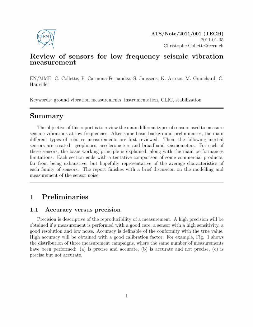
Precision is descriptive of the reproducibility of a measurement. A high precision will beobtained if a measurement is performed with a good care, a sensor with a high sensitivity, agood resolution and low noise. Accuracy is definable of the conformity with the true value.High accuracy will be obtained with a good calibration factor. For example, Fig. 1 showsthe distribution of three measurement campaigns, where the same number of measurementshave been performed: (a) is precise and accurate, (b) is accurate and not precise, (c) isprecise but not accurate.

1

Measurement

distribution

Value

True

(a)

(b)

(c)

Figure 1: Accuracy versus precision.

1.2 Propagation of errors

If M is a measured value, and EM is the error on this measurement, then the measuredvalue Mmeas is comprised in a range of

Mmeas = M ± EM (1)

In this section, we give the general formulas to evaluate the error in the result of simplemathematical operations performed with measured values, assuming gaussian error distri-butions. A detailed treatment of this topic can be found in [1].

• Addition and substraction Following Equ.(1), the error in the addition of twomeasured values is given by

Esum =√

E2A + E2

B (2)

where EA and EB are the errors of the two quantities A and B. Similarly, the erroron the difference is given by

Ediff = ±√

E2A + E2

B (3)

• Multiplication

Eprod = AB

√(E2

A

A)2 + (

E2B

B)2 (4)

• Division

Ediv =A

B

√(E2

A

A)2 + (

E2B

B)2 (5)

2

• Power and root From Equ.(4), we have directly

Epower = An

√n(

EA

A)2 =

EA

AAn

√n = EAA

n−1√n (6)

However, this assumes that the value of EA may change each time A is used, whichis actually not he case; once the measurement of A has been completed, the error EA

is fixed. Hence, the correct expression is made if we note that EA is involved n timesand not

√n times. Thus,

Epower = nAn

√(EA

A)2 = EAnA

n−1 (7)

Similarly, the error in the nth root is

Eroot =1

nE

1/n−1A (8)

1.3 Sensitivity, noise and resolution

The resolution is the smallest quantity that one can measure. It is defined as the ratiobetween the noise and the sensitivity. If the sensor measures a displacement, the resolutionis

Resolution[m√Hz

] =Noise[ V√

Hz]

Sensitivity[Vm]

(9)

The main sources of sensor noise are presented in section 4.1.

2 Relative measurement

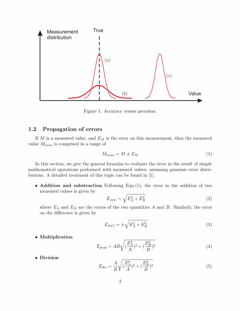
The main relative measurement sensors used in seismic sensors are Linear Variable Dif-ferential Transformer (LVDT), Eddy current sensors, capacitive sensors, interferometers andBragg fibers. A comparison of these technologies can be found in [2, 3]. Their main charac-teristics are summarized in Table 1.

Eddy current and LVDT are linear over a long distance, low cost and rather high precision.Unfortunately, because of their principle is based on magnetic field, they cannot work in anenvironment where there is a stray magnetic field (e.g. a particle accelerator). Capacitivegauges have a very low noise floor, are easy to mount and not expensive. The main restrictionfor their use is a small stroke to maintain a good resolution, linearity, and precise parallelismbetween the two plates. They are widely used in broadband seismometers. Interferometers,encoders and Bragg fibers are optical sensors. They don’t suffer from a loss of resolution forlarge displacements but, except from encoders, are much more expensive.

3

Technology Freq. Resolution Range Size T range Refs.(Hz) nm RMS (cm) 0C

LVDT DC-200 10 1-10 mm 1 −50, 100 [4]Eddy cur. 5 k 0.1-100 0.5-50 mm 1 −50, 100 [5]Capacitive DC-100k 0.05-50 50nm-1cm 0.5-1 −40, 120 [6, 7, 8]

Interferometer 300 k 0.1 10cm 1 −250, 100 [9, 10]Encoder DC-1M 1 7-27 3x3,5 0-40 [11]

Bragg Fibers DC-150 0.3 3.5 mm 10 −30, 80 [12, 13, 14]

Table 1: Characteristics of relative measurement sensors.

3 Absolute measurement

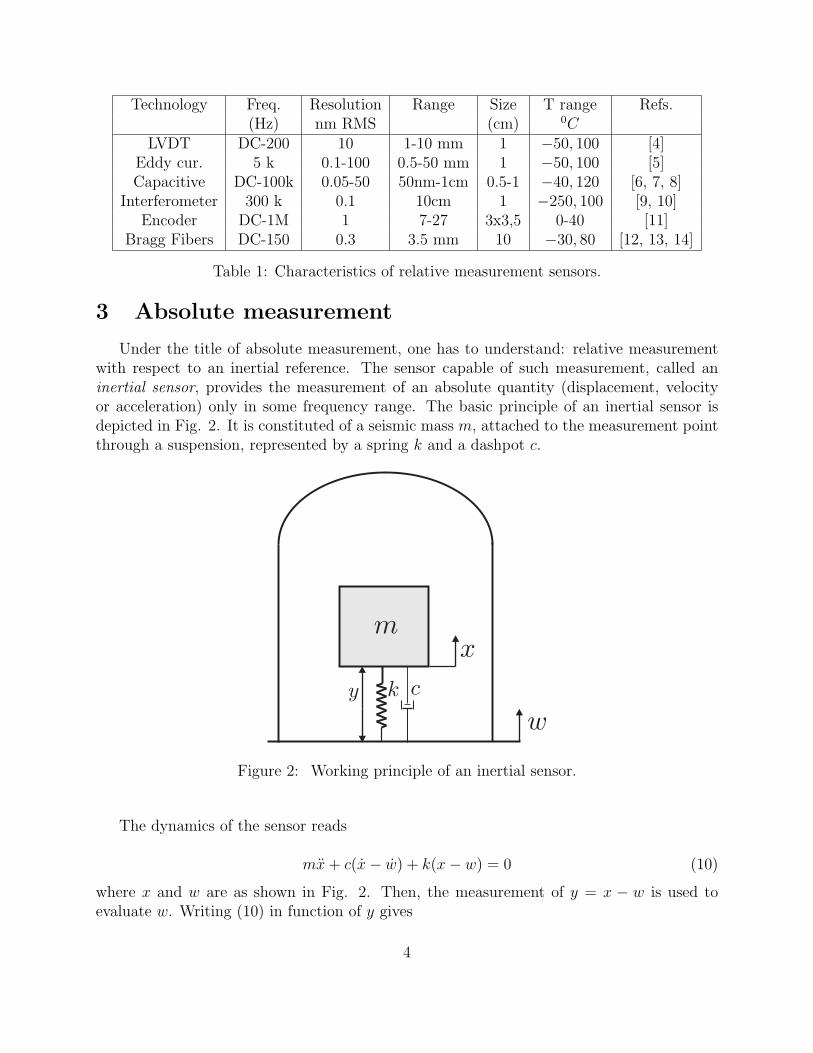
Under the title of absolute measurement, one has to understand: relative measurementwith respect to an inertial reference. The sensor capable of such measurement, called aninertial sensor, provides the measurement of an absolute quantity (displacement, velocityor acceleration) only in some frequency range. The basic principle of an inertial sensor isdepicted in Fig. 2. It is constituted of a seismic mass m, attached to the measurement pointthrough a suspension, represented by a spring k and a dashpot c.

Figure 2: Working principle of an inertial sensor.

The dynamics of the sensor reads

mx+ c(x− w) + k(x− w) = 0 (10)

where x and w are as shown in Fig. 2. Then, the measurement of y = x − w is used toevaluate w. Writing (10) in function of y gives

4

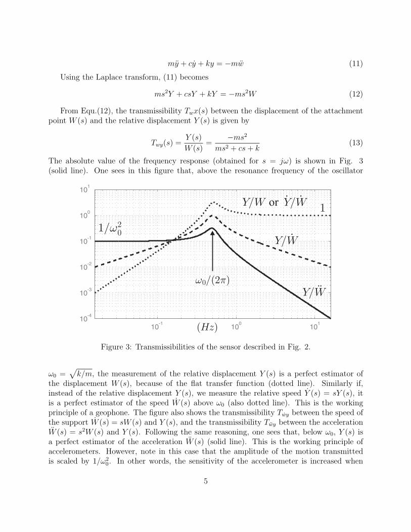
my + cy + ky = −mw (11)

Using the Laplace transform, (11) becomes

ms2Y + csY + kY = −ms2W (12)

From Equ.(12), the transmissibility Twx(s) between the displacement of the attachmentpoint W (s) and the relative displacement Y (s) is given by

Twy(s) =Y (s)

W (s)=

−ms2

ms2 + cs+ k(13)

The absolute value of the frequency response (obtained for s = jω) is shown in Fig. 3(solid line). One sees in this figure that, above the resonance frequency of the oscillator

Figure 3: Transmissibilities of the sensor described in Fig. 2.

ω0 =√

k/m, the measurement of the relative displacement Y (s) is a perfect estimator ofthe displacement W (s), because of the flat transfer function (dotted line). Similarly if,instead of the relative displacement Y (s), we measure the relative speed Y (s) = sY (s), itis a perfect estimator of the speed W (s) above ω0 (also dotted line). This is the workingprinciple of a geophone. The figure also shows the transmissibility Twy between the speed ofthe support W (s) = sW (s) and Y (s), and the transmissibility Twy between the accelerationW (s) = s2W (s) and Y (s). Following the same reasoning, one sees that, below ω0, Y (s) isa perfect estimator of the acceleration W (s) (solid line). This is the working principle ofaccelerometers. However, note in this case that the amplitude of the motion transmittedis scaled by 1/ω2

0. In other words, the sensitivity of the accelerometer is increased when

5

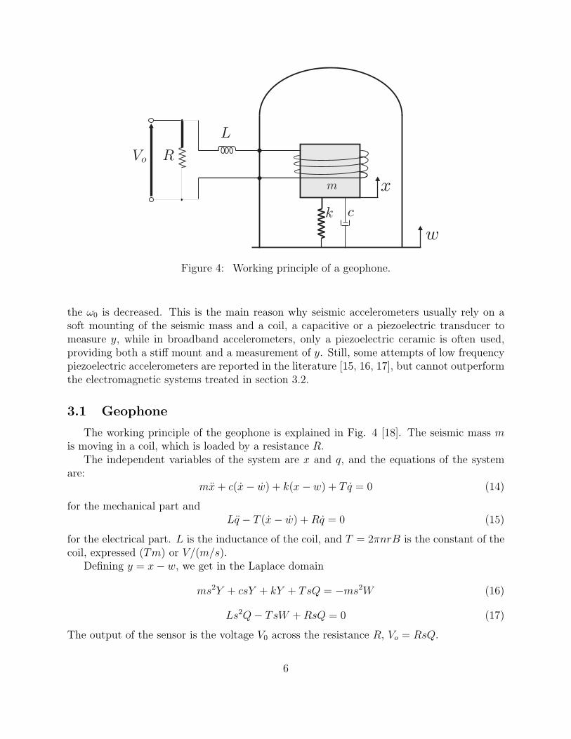
Figure 4: Working principle of a geophone.

the ω0 is decreased. This is the main reason why seismic accelerometers usually rely on asoft mounting of the seismic mass and a coil, a capacitive or a piezoelectric transducer tomeasure y, while in broadband accelerometers, only a piezoelectric ceramic is often used,providing both a stiff mount and a measurement of y. Still, some attempts of low frequencypiezoelectric accelerometers are reported in the literature [15, 16, 17], but cannot outperformthe electromagnetic systems treated in section 3.2.

3.1 Geophone

The working principle of the geophone is explained in Fig. 4 [18]. The seismic mass mis moving in a coil, which is loaded by a resistance R.

The independent variables of the system are x and q, and the equations of the systemare:

mx+ c(x− w) + k(x− w) + T q = 0 (14)

for the mechanical part andLq − T (x− w) +Rq = 0 (15)

for the electrical part. L is the inductance of the coil, and T = 2πnrB is the constant of thecoil, expressed (Tm) or V/(m/s).

Defining y = x− w, we get in the Laplace domain

ms2Y + csY + kY + TsQ = −ms2W (16)

Ls2Q− TsW +RsQ = 0 (17)

The output of the sensor is the voltage V0 across the resistance R, Vo = RsQ.

6

Vo

sW=

RT

Ls+R

−ms2

ms2 + sc+ k + TsLs+R

(18)

If R is large, Equ.(3.1) is reduced to

Vo

sW=

−mTs2

ms2 + sc+ k=

−Ts2

s2 + 2ξgωgs+ ω2g

(19)

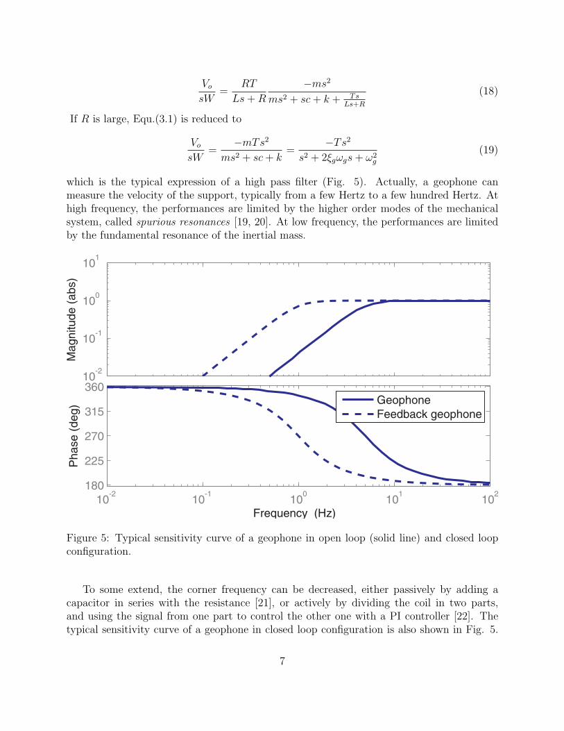
which is the typical expression of a high pass filter (Fig. 5). Actually, a geophone canmeasure the velocity of the support, typically from a few Hertz to a few hundred Hertz. Athigh frequency, the performances are limited by the higher order modes of the mechanicalsystem, called spurious resonances [19, 20]. At low frequency, the performances are limitedby the fundamental resonance of the inertial mass.

Figure 5: Typical sensitivity curve of a geophone in open loop (solid line) and closed loopconfiguration.

To some extend, the corner frequency can be decreased, either passively by adding acapacitor in series with the resistance [21], or actively by dividing the coil in two parts,and using the signal from one part to control the other one with a PI controller [22]. Thetypical sensitivity curve of a geophone in closed loop configuration is also shown in Fig. 5.

7

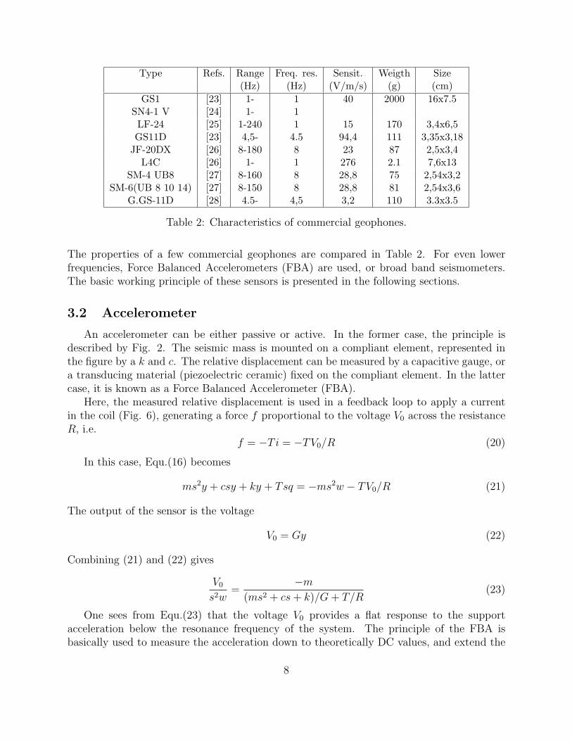
Type Refs. Range Freq. res. Sensit. Weigth Size(Hz) (Hz) (V/m/s) (g) (cm)

GS1 [23] 1- 1 40 2000 16x7.5SN4-1 V [24] 1- 1LF-24 [25] 1-240 1 15 170 3,4x6,5GS11D [23] 4,5- 4.5 94,4 111 3,35x3,18JF-20DX [26] 8-180 8 23 87 2,5x3,4

L4C [26] 1- 1 276 2.1 7,6x13SM-4 UB8 [27] 8-160 8 28,8 75 2,54x3,2

SM-6(UB 8 10 14) [27] 8-150 8 28,8 81 2,54x3,6G.GS-11D [28] 4.5- 4,5 3,2 110 3.3x3.5

Table 2: Characteristics of commercial geophones.

The properties of a few commercial geophones are compared in Table 2. For even lowerfrequencies, Force Balanced Accelerometers (FBA) are used, or broad band seismometers.The basic working principle of these sensors is presented in the following sections.

3.2 Accelerometer

An accelerometer can be either passive or active. In the former case, the principle isdescribed by Fig. 2. The seismic mass is mounted on a compliant element, represented inthe figure by a k and c. The relative displacement can be measured by a capacitive gauge, ora transducing material (piezoelectric ceramic) fixed on the compliant element. In the lattercase, it is known as a Force Balanced Accelerometer (FBA).

Here, the measured relative displacement is used in a feedback loop to apply a currentin the coil (Fig. 6), generating a force f proportional to the voltage V0 across the resistanceR, i.e.

f = −Ti = −TV0/R (20)

In this case, Equ.(16) becomes

ms2y + csy + ky + Tsq = −ms2w − TV0/R (21)

The output of the sensor is the voltage

V0 = Gy (22)

Combining (21) and (22) gives

V0

s2w=

−m

(ms2 + cs+ k)/G+ T/R(23)

One sees from Equ.(23) that the voltage V0 provides a flat response to the supportacceleration below the resonance frequency of the system. The principle of the FBA isbasically used to measure the acceleration down to theoretically DC values, and extend the

8

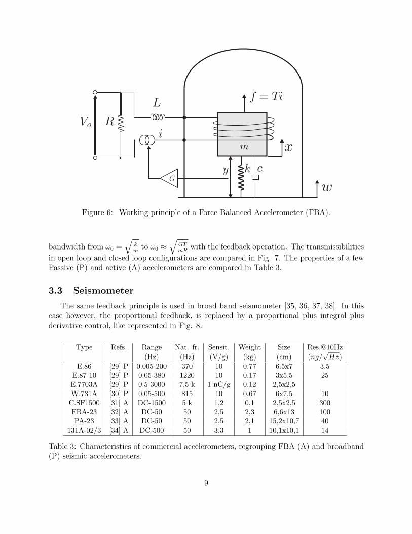
Figure 6: Working principle of a Force Balanced Accelerometer (FBA).

bandwidth from ω0 =√

kmto ω0 ≈

√GTmR

with the feedback operation. The transmissibilities

in open loop and closed loop configurations are compared in Fig. 7. The properties of a fewPassive (P) and active (A) accelerometers are compared in Table 3.

3.3 Seismometer

The same feedback principle is used in broad band seismometer [35, 36, 37, 38]. In thiscase however, the proportional feedback, is replaced by a proportional plus integral plusderivative control, like represented in Fig. 8.

Type Refs. Range Nat. fr. Sensit. Weight Size Res.@10Hz

(Hz) (Hz) (V/g) (kg) (cm) (ng/√Hz)

E.86 [29] P 0.005-200 370 10 0.77 6.5x7 3.5E.87-10 [29] P 0.05-380 1220 10 0.17 3x5,5 25E.7703A [29] P 0.5-3000 7,5 k 1 nC/g 0,12 2,5x2,5W.731A [30] P 0.05-500 815 10 0,67 6x7,5 10C.SF1500 [31] A DC-1500 5 k 1,2 0,1 2,5x2,5 300FBA-23 [32] A DC-50 50 2,5 2,3 6,6x13 100PA-23 [33] A DC-50 50 2,5 2,1 15,2x10,7 40

131A-02/3 [34] A DC-500 50 3,3 1 10,1x10,1 14

Table 3: Characteristics of commercial accelerometers, regrouping FBA (A) and broadband(P) seismic accelerometers.

9

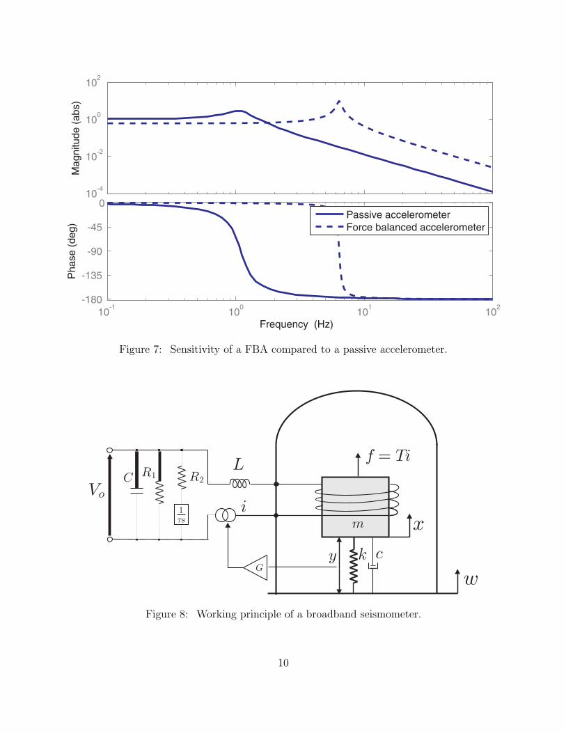
Figure 7: Sensitivity of a FBA compared to a passive accelerometer.

Figure 8: Working principle of a broadband seismometer.

10

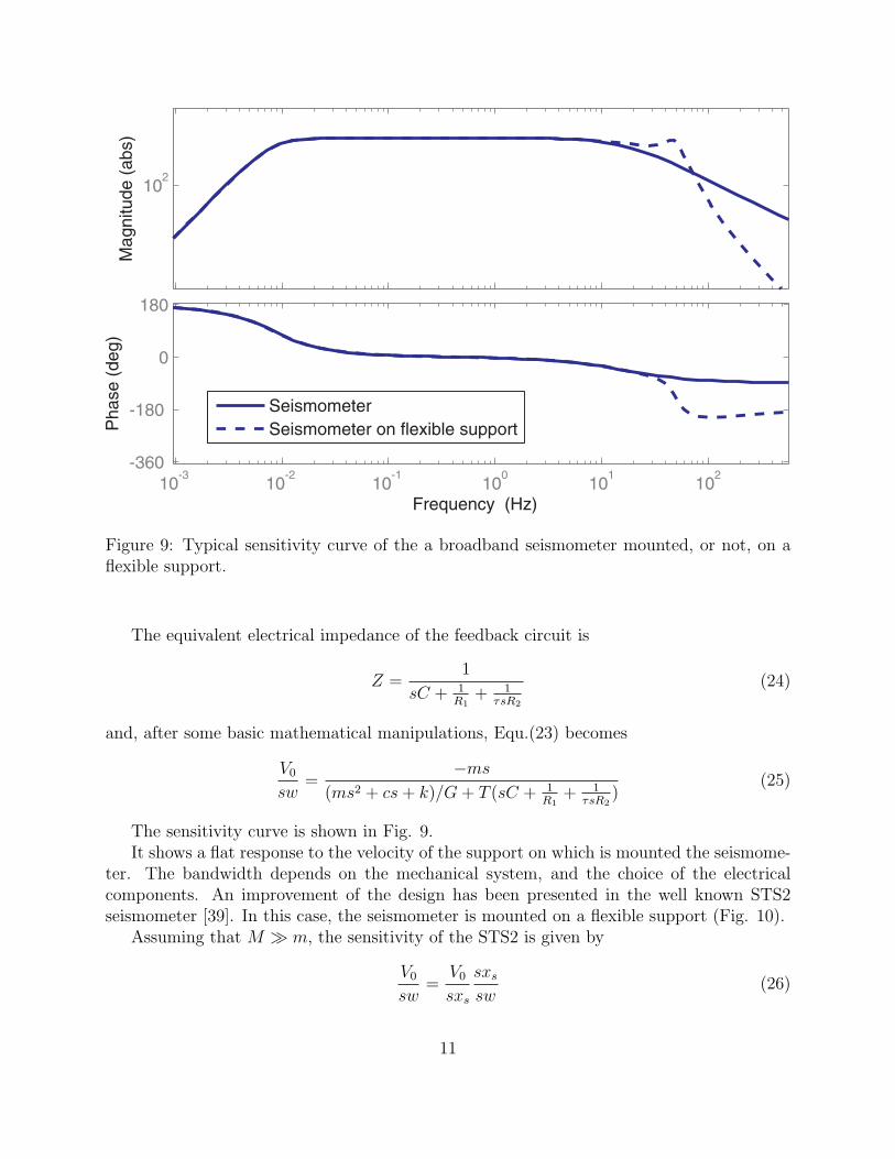
Figure 9: Typical sensitivity curve of the a broadband seismometer mounted, or not, on aflexible support.

The equivalent electrical impedance of the feedback circuit is

Z =1

sC + 1R1

+ 1τsR2

(24)

and, after some basic mathematical manipulations, Equ.(23) becomes

V0

sw=

−ms

(ms2 + cs+ k)/G+ T (sC + 1R1

+ 1τsR2

)(25)

The sensitivity curve is shown in Fig. 9.It shows a flat response to the velocity of the support on which is mounted the seismome-

ter. The bandwidth depends on the mechanical system, and the choice of the electricalcomponents. An improvement of the design has been presented in the well known STS2seismometer [39]. In this case, the seismometer is mounted on a flexible support (Fig. 10).

Assuming that M ≫ m, the sensitivity of the STS2 is given by

V0

sw=

V0

sxs

sxs

sw(26)

11

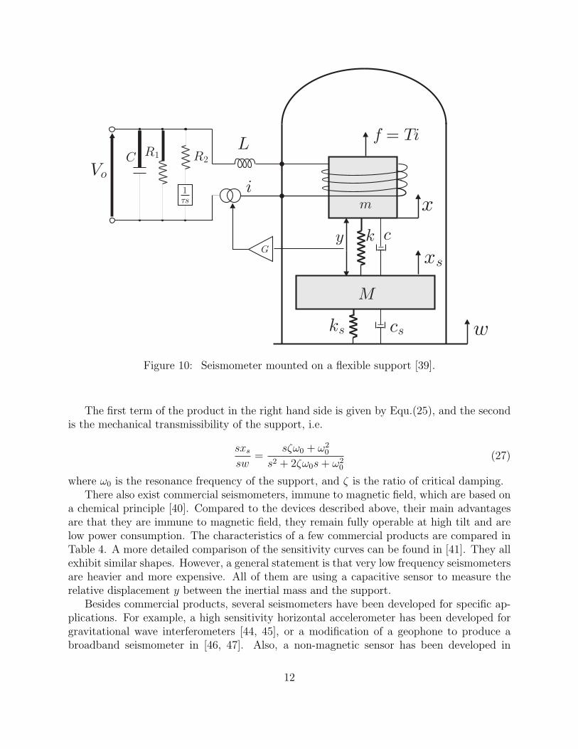
Figure 10: Seismometer mounted on a flexible support [39].

The first term of the product in the right hand side is given by Equ.(25), and the secondis the mechanical transmissibility of the support, i.e.

sxs

sw=

sζω0 + ω20

s2 + 2ζω0s+ ω20

(27)

where ω0 is the resonance frequency of the support, and ζ is the ratio of critical damping.There also exist commercial seismometers, immune to magnetic field, which are based on

a chemical principle [40]. Compared to the devices described above, their main advantagesare that they are immune to magnetic field, they remain fully operable at high tilt and arelow power consumption. The characteristics of a few commercial products are compared inTable 4. A more detailed comparison of the sensitivity curves can be found in [41]. They allexhibit similar shapes. However, a general statement is that very low frequency seismometersare heavier and more expensive. All of them are using a capacitive sensor to measure therelative displacement y between the inertial mass and the support.

Besides commercial products, several seismometers have been developed for specific ap-plications. For example, a high sensitivity horizontal accelerometer has been developed forgravitational wave interferometers [44, 45], or a modification of a geophone to produce abroadband seismometer in [46, 47]. Also, a non-magnetic sensor has been developed in

12

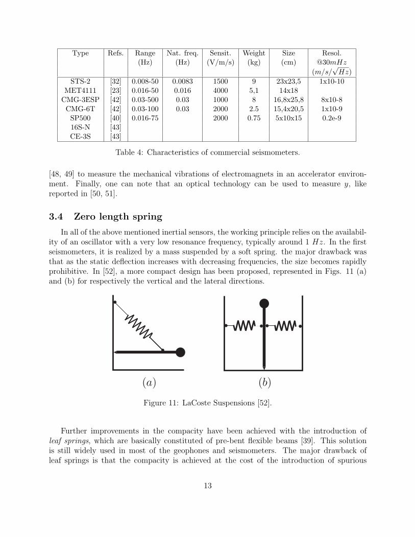
Type Refs. Range Nat. freq. Sensit. Weight Size Resol.(Hz) (Hz) (V/m/s) (kg) (cm) @30mHz

(m/s/√Hz)

STS-2 [32] 0.008-50 0.0083 1500 9 23x23,5 1x10-10MET4111 [23] 0.016-50 0.016 4000 5,1 14x18CMG-3ESP [42] 0.03-500 0.03 1000 8 16,8x25,8 8x10-8CMG-6T [42] 0.03-100 0.03 2000 2.5 15,4x20,5 1x10-9SP500 [40] 0.016-75 2000 0.75 5x10x15 0.2e-916S-N [43]CE-3S [43]

Table 4: Characteristics of commercial seismometers.

[48, 49] to measure the mechanical vibrations of electromagnets in an accelerator environ-ment. Finally, one can note that an optical technology can be used to measure y, likereported in [50, 51].

3.4 Zero length spring

In all of the above mentioned inertial sensors, the working principle relies on the availabil-ity of an oscillator with a very low resonance frequency, typically around 1 Hz. In the firstseismometers, it is realized by a mass suspended by a soft spring. the major drawback wasthat as the static deflection increases with decreasing frequencies, the size becomes rapidlyprohibitive. In [52], a more compact design has been proposed, represented in Figs. 11 (a)and (b) for respectively the vertical and the lateral directions.

Figure 11: LaCoste Suspensions [52].

Further improvements in the compacity have been achieved with the introduction ofleaf springs, which are basically constituted of pre-bent flexible beams [39]. This solutionis still widely used in most of the geophones and seismometers. The major drawback ofleaf springs is that the compacity is achieved at the cost of the introduction of spurious

13

resonances [19, 20], requiring a careful design. The second frequency of an oscillator with afundamental resonance at a few Hertz is typically around 200 Hz. In [53, 54], an interestingalternative has been presented, where a horizontal seismometer has been developed usinga folded pendulum. It uses flexural joints, and a tunable fundamental frequency, stronglydecoupled from the higher order modes. Other interesting devices are presented in [55] wherethe rotative inertial mass has a V-shape to improve the sensitivity, or in [56, 57] where a lowfrequency oscillator is achieved with an anti-spring.

4 Sensor noise

The noise floor of a sensor is one of the main factors limiting the performances of vibrationisolation strategies, especially for those who do not rely on passive isolation, i.e. active hardmounts [58, 59, 60, 61]. The main sources of noise will be first reviewed in the next section.Then, a general method to evaluate experimentally the sensor noise will be presented, andillustrated with numerical and experimental examples.

4.1 Sources of Noise

Ground motion sensors are all based on the measurement of the relative motion of aproof mass with respect to the ground. In such sensors, there exists basically four differentsources of noise [3, 62, 63]:

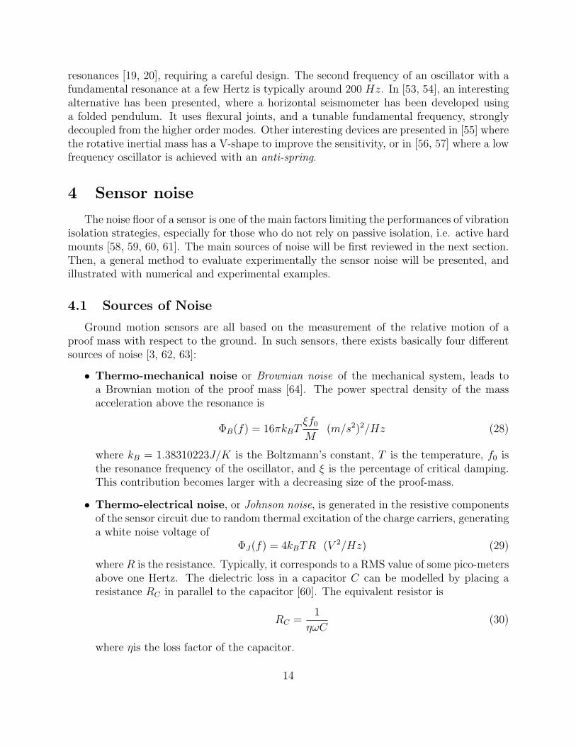
• Thermo-mechanical noise or Brownian noise of the mechanical system, leads toa Brownian motion of the proof mass [64]. The power spectral density of the massacceleration above the resonance is

ΦB(f) = 16πkBTξf0M

(m/s2)2/Hz (28)

where kB = 1.38310223J/K is the Boltzmann’s constant, T is the temperature, f0 isthe resonance frequency of the oscillator, and ξ is the percentage of critical damping.This contribution becomes larger with a decreasing size of the proof-mass.

• Thermo-electrical noise, or Johnson noise, is generated in the resistive componentsof the sensor circuit due to random thermal excitation of the charge carriers, generatinga white noise voltage of

ΦJ(f) = 4kBTR (V 2/Hz) (29)

where R is the resistance. Typically, it corresponds to a RMS value of some pico-metersabove one Hertz. The dielectric loss in a capacitor C can be modelled by placing aresistance RC in parallel to the capacitor [60]. The equivalent resistor is

RC =1

ηωC(30)

where ηis the loss factor of the capacitor.

14

• Shot noise or Schottky noise is caused by random movement of electric charges acrosspotential barriers, such as p-n junctions [63]. Its power spectral density Φsh(f) can bemodelled by

Φsh(f) = 2qIdc (A2/Hz) (31)

where Idc is the average current that crosses the barrier. It has the shape of a whitenoise current.

• Flicker noise or 1/f noise is mainly due to impurities in the production of semicon-ductor devices. Its main characteristic is that its power spectral density is inverselyproportional to the frequency, and can be modelled by

ΦV (f) = K/fα (V 2/Hz) (32)

where the exponent is usually α = 1. Typical values for sensor amplifier’s noise con-stants can be found in [60].

• Discretization noise

As these sources of noise are uncorrelated, the overall sensor noise floor Φnn(f) can bedirectly estimated by summing all of the contributions as

Φnn(f) = ΦB(f) +G2{ΦJ(f) + Z2(f)Φsh(f) + ΦV (f)} (33)

where Z(f) is the load at which the current noise is developed, and G is the sensitivity,converting the voltage (V ) into acceleration (m2/s). The next section provides a tool toevaluate the magnitude of the overall noise arising from a set of sensors and amplifier.

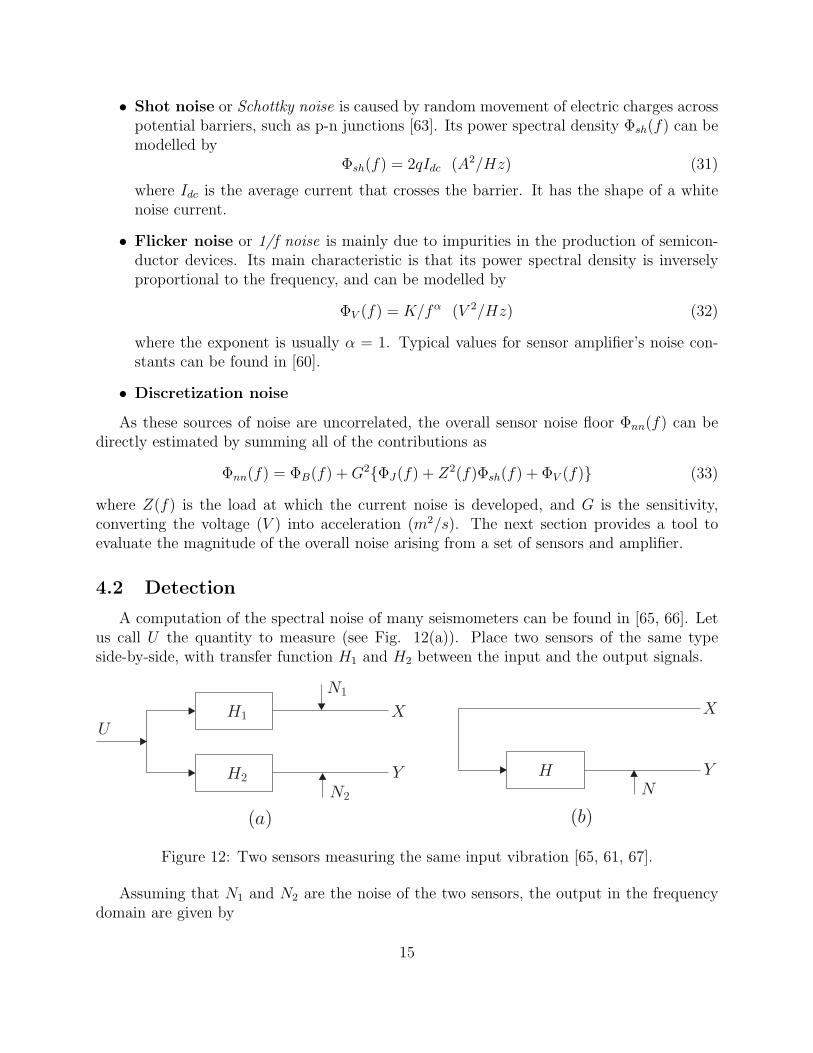
4.2 Detection

A computation of the spectral noise of many seismometers can be found in [65, 66]. Letus call U the quantity to measure (see Fig. 12(a)). Place two sensors of the same typeside-by-side, with transfer function H1 and H2 between the input and the output signals.

U

H1

H2

N1

N2

X

Y H

N

X

Y

(a) (b)

Figure 12: Two sensors measuring the same input vibration [65, 61, 67].

Assuming that N1 and N2 are the noise of the two sensors, the output in the frequencydomain are given by

15

X(ω) = H1(ω)U(ω) +N1(ω) (34)

Y (ω) = H2(ω)U(ω) +N2(ω) (35)

The coherence between the two signals is given by

γ(ω) =Φxy(ω)√

Φxx(ω)Φyy(ω)(36)

Resolving Equ.(34) for U(ω) and replacing into Equ.(35) gives

Y (ω) = H(ω)X(ω) +N(ω) (37)

where H(ω) = H2(ω)/H1(ω) and N(ω) = N2(ω) −H(ω)N1(ω). The corresponding schemeis given in Fig. 12(b), and

H(ω) =Φxy

Φxx

(38)

From Equ.(37), we find

Φss = H2Φxx = Φxxγ2(ω) (39)

Φnn = Φyy −H2Φxx (40)

β(ω) =Φss

Φnn

=ΦxxH

2

Φnn

=γ2

1− γ2(41)

which are respectively the noise power spectrum, the signal spectrum and signal to noiseratio. The RMS value of the noise and signal are given respectively by

σn(ω) = [

∫ ∞

ω

Φnn(ν)dν]1/2 (42)

and

σs(ω) = [

∫ ∞

ω

Φss(ν)dν]1/2 (43)

These last two equations provide a tool to evaluate the capacity of a sensor to detect asignal u(t) in the frequency range of interest.

Figure 13 compares the noise floor of several sensors: geophone L4C [26], seismometerCMG 6T [42], capacitive [68], and interferometric [54, 9]. At low frequency, the 1/f noise isinherent to the electronic circuity. At higher frequency, capacitive sensors have a resolutionabout 10 times better than magnetic sensors, and interferometric sensors further improvethe resolution by another factor 10.

16

Figure 13: Comparison of sensor noise floor.

5 Conclusion

In this report, the main types of inertial sensors have been reviewed: accelerometers,geophones, and seismometers. For each of them, the characteristics of a few commercialproducts have been compared. Then, it has been followed by a brief discussion on thepractical realization of the mechanical system, and on the sources of noise. It has beenshown that, among all commercial products, optical interferometer shows currently the bestnoise figure.

References

[1] B. Barry. Errors in practical measurement in science, engineering and technology. Wiley,1978.

[2] L. Zuo. Element and System Design for Active and Passive Vibration Isolation. PhDthesis, Massachusetts Institute of Technology, Novemeber 2004.

[3] Zeroth-order design report for the next linear collider, slac report 474.

[4] MacroSensors. http://www.macrosensors.com/.

[5] Kaman Systems. http://www.kamansensors.com/.

17

[6] C. Acar and A.M. Shkel. Experimental evaluation and comparative analysis of com-mercial variable-capacitance mems accelerometers. J. Micromech. Microeng., 13:634645,2003.

[7] Lion Precision. http://www.lionprecision.com/.

[8] Fogale nanotech. http://www.fogale.com/.

[9] Attocube systems AG. http://www.attocube.com/.

[10] M.S. Warden, P.A. Coe, and A. Reichold. Nanometer precision interferometric stabilitymonitoring systems for key accelerator components. In Proceedings of the EPAC 08,Genoa (Italy), 2008.

[11] HEIDENHAIN CORPORATION. http://www.heidenhain.com/.

[12] Optical Fibers. http://www.opticalfibersensors.org/.

[13] P. Ferraro and G. De Natale. On the possible use of optical fiber bragg gratings asstrain sensors for geodynamical monitoring. Optics and Lasers in Engineering, 37:115–130, 2002.

[14] A. Gerardin, M. Guinchard, A. Kuzmin, and K.-H. Haase. Use of the optical straingauges and temperature sensors based on fiber gratings at cryogenic temperatures.Technical Report CERN EN-MME Mechanical Measurement Lab Report, EDMS No:1103571, 2010.

[15] C.-H. Liu and T.W. Kenny. A high precision, wide-bandwidth micromachined tunnelingaccelerometer. Journal of microelectromechanical systems, 10(3):425–433, 2001.

[16] B.L.F. Daku, E.M.A. Mohamed, and A.F. Prugger. A PVDF transducer for low-frequency acceleration measurements. ISA transactions, 43:319–328, 2004.

[17] A.T. Kollias and J.N. Avaritsiotis. A study of the performance of bending mode piezo-electric accelerometers. Sensors and actuators, 121:434–442, 2005.

[18] X. Roset, J. del Rio, A. Manuel, and R. Palomera-Garcia. Contributions to modelcharacterization of geophone sensor. Instrumentation and Measurement TechnologyConfcrence IMTC 2004 (Como, Italy), 2004.

[19] F.H. Ling, W.M. Wang, and R.J. Mao. Dynamic stability analysis of the geophonespurious frequency phenomenon. Journal of Sound and Vibration, 139(1):21–30, 1990.

[20] K. Faber and P.W. Maxwell. Geophone spurious frequency: what is it and how does itaffect seismic data quality ? Canadian Journal of Exploration Geophysics, 33(1):46–54,1997.

18

[21] A. Pazos, G. Alguacil, and J. Martin Davila. A simple technique to extend the band-width of electromagnetic sensors. Bulletin of the Seismological Society of America, 2005.

[22] A. Preumont. Mechatronics, Dynamics of Electromechanical and Piezoelectric Systems.Springer, 2006.

[23] Sara. http://www.sara.pg.it/.

[24] Gisco. http://www.gisco.com/.

[25] Input/Output SENSOR Nederland. http://www.i-o.com/.

[26] Secrel France. http://www.sercel.com/en/.

[27] Sensor. http://www.geophone.com/.

[28] Geospace. http://www.Geospace.com/.

[29] Endevco. http://www.endevco.com/.

[30] Wilcoxon. http://www.wilcoxon.com/.

[31] Colibrys. http://www.colibrys.com/.

[32] Kinemetrics Inc. http://www.kinemetrics.com/.

[33] Geotech Instruments LLC. http://www.geoinstr.com.

[34] Refraction Technology Inc. http://www.reftek.com/.

[35] H. E. Sheffield. An electronic vertical long-period seismometer. Instrumentation andMeasurement, IEEE Transactions on, 13(1):2 –7, 1964.

[36] M.J. Usher, R.F. Burch, and C. Guralp. Wide-band feedback seismometers. Physics ofthe Earth and Planetary Interiors, 18:38–50, 1979.

[37] B.S Melton and D.P. Johnson. Inertial seismograph design - limitations in principle andpractice (or how not to build a sensitive seismograph). Proceedings of the IRE, pages2328–2339, 1962.

[38] C. Teupser and A. Plesinger. Design of feedback-controlled wide-band seismographswith respect to undesired side-effects. Physics of the Earth and Planetary Interiors,18:58–63, 1979.

[39] E. Wielandt and G. Sterkeisen. The leaf spring seismometer: design and performance.Bulletin of the Seismological Society of America, 1982.

[40] PMD SCIENTIFIC INC. http://www.eentec.com.

19

[41] http://www.passcal.nmt.edu/content/instrumentation/sensors/.

[42] Guralp. Guralp catalogue.

[43] Pasi. http://www.eng.pasigeophysics.com/.

[44] A. Bertolini, R. DeSalvo, F. Fidecaro, M. Francesconi, S. Marka, V. Sannibale, D. Si-monetti, A. Takamori, and H. Tariq. Mechanical design of a single-axis monolithic ac-celerometer for advanced seismic sttenuation systems. Nuclear Instruments and Methodsin Physics Research A, 556:616–623, 2006.

[45] A. Bertolini, R. DeSalvo, F. Fidecaro, M. Francesconi, S. Marka, V. Sannibale, D. Si-monetti, A. Takamori, and H. Tariq. Mechanical design of a single-axis monolithic ac-celerometer for advanced seismic sttenuation systems. Nuclear Instruments and Methodsin Physics Research A, 564:579–586, 2006.

[46] A. Barzilai, T. VanZandt, T. Pike, S. Manionand, and T. Kenny. Improving the perfor-mances of a geophone through capacitive position sensing and feedback. In AmericanSociety of Mechanical Engineers International Congress, 1998.

[47] A. Brazilai. Improving a Geophone to Produce an Affordable, Broadband Seismometer.PhD thesis, Stanford University, January 2000.

[48] J. Frisch, E. Doyle, L. Eriksson, L. Hendrickson, T. Himel, T. Markiewicz, and R. Par-tridge. Inertial sensor development for active vibration stabilization. IEEE ParticleAccelerator Conference, 2003.

[49] J. Frisch, V. Decker, E. Doyle, L. Hendrickson, T. Himel, T. Markiewicz, and A. Seryi.Development of a non-magnetic inertial sensor for vibration stabilization in a linearcollider. In 22nd International Linear Collider Conference, 16-18 August (Germany),2004.

[50] D. Gardner, T. Hofler, S. Baker, R. Yarber, and S. Garrett. A fiber-optic interferometricseismometer. Lightwave Technology, Journal of, 5(7):953 – 960, July 1987.

[51] M. Zumberge, J. Berger, J. Otero, and E. Wielandt. An optical seismometer withoutforce feedback. Bulletin of Seismological Society of America, 100(2):598–605, 2010.

[52] L.J.B. LaCoste. A new type of long period seismograph. Physics, 1934.

[53] F. Acernese, G. Giordano, R. Romano, R. De Rosa, and F. Barone. Mechanical mono-lithic horizontal sensor for low frequency seismic noise measurement. Review of Scientificinstruments, 79:074501, 2008.

[54] F. Acernese, G. Giordano, R. Romano, R. De Rosa, and F. Barone. Tunable mechanicalmonolithic sensor with interferometric readout for low frequency seismic noise measure-ment. Nuclear Instruments and Methods in Physics Research A, 617:457–458, 2008.

20

[55] S. Cacho, P. Lognonne, J. F. Karczewski, G. Pont, and G. Coste. A very broad band 3axis seismometer to study internal structure of mars. Space Mechanisms and Tribology,Proceedings of the 8th European Symposium, 1999.

[56] A. Bertolini, G. Cella, R. DeSalvo, and V. Sannibale. Seismic noise filters, verticalresonance frequency reduction with geometric anti-springs: a feasibility study. NuclearInstruments and Methods in Physics Research A, 435:475–483, 1999.

[57] A. Bertolini, N. Beverini, G. Cella, R. De Salvo, F. Fidecaro, M. Francesconi, andD. Somonetti. Geometric anti-spring vertical accelerometers for seismic monitoring.Nuclear Instruments and Methods in Physics Research A, 518:233–235, 2004.

[58] C. Collette, K. Artoos, A. Kuzmin, S. Janssens, M. Sylte, M. Guinchard, andC. Hauviller. Active quadrupole stabilization for future linear particle colliders. NuclearInstruments and Methods in Physics Research A, 621(1-3):71–78, 2010.

[59] T. van der Poel, J. van Dijk, B. Jonker, and H. Soemers. Improving the vibrationisolation performance of hard mounts for precision equipment. In Advanced intelligentmechatronics, 2007 ieee/asme international conference on, pages 1 –5, 4-7 2007.

[60] G.W. van der Poel. An exploration of active hard mount vibration isolation for precisionequipment. PhD thesis, University of Twente, 2010.

[61] C. Montag. Active stabilization of mechanical quadrupole vibrations for linear collider.Nuclear Instruments and Methods in Physics Research A, 378:396–375, 1996.

[62] A. Barzilai, T. VanZandt, and T. Kenny. Technique for measurement of the noise ofa sensor in the presence of large background signals. Review of scientific instruments,69:2767–2772, 1998.

[63] R. Pallas-Areny and J.G. Webster. Sensors and signal conditioning. John Wiley, 2001.

[64] S. Rowan, J. Hough, and D.R.M. Crooks. Thermal noise and material issues for gravi-tational wave detectors. Physics Letters A, 347:25–32, 2005.

[65] L.G. Holcomb. A direct method for calculating instrument noise levels in side-by-sideseismometer evaluations. Technical Report 89-214, United States Department of theInterior Geological Survey, 1989.

[66] P.W. Rodgers. Self-noise spectra for 34 common electromagnetic seismome-ter/preamplifier pairs. Bulletin of the Seismological society of America, 1994.

[67] C. Montag. Active Stabilization of Mechanical Quadrupole Vibrations in a Linear Col-lider Test Facility. PhD thesis, Hamburg University, 1996.

[68] Physik Instrumente (PI) GmbH & Co. P-225, p-235 pica? power piezo stack actuatorspreloaded high-load piezo actuators (hvpzt) w/ sensor option.

21