C. Population Density 2. Habitat Selection
32
C. Population Density 2. Habitat Selection
description
C. Population Density 2. Habitat Selection. C. Population Density 3. Maintenance of Marginal Populations. Why don’t these adapt to local conditions?. D. Modeling the Spatial Structure of Populations 1. Metapopulation Model. - PowerPoint PPT Presentation
Transcript of C. Population Density 2. Habitat Selection
C. Population Density 2. Habitat Selection

C. Population Density 3. Maintenance of Marginal Populations
Why don’t these adapt to local conditions?
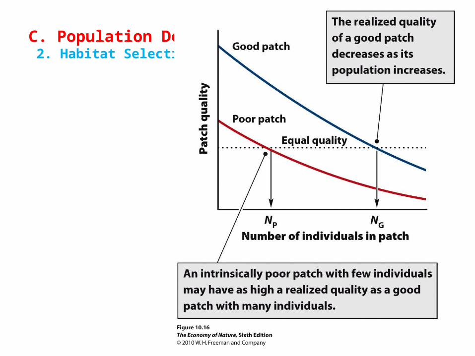
D. Modeling the Spatial Structure of Populations 1. Metapopulation Model
Subpopulation inhabit separate patches of the same habitat type in a “matrix” of inhospitable habitat..
- immigration causes recolonization of habitats in which population went extinct. So, rates of immigration and local extinction are critical to predicting long-term viability of population.
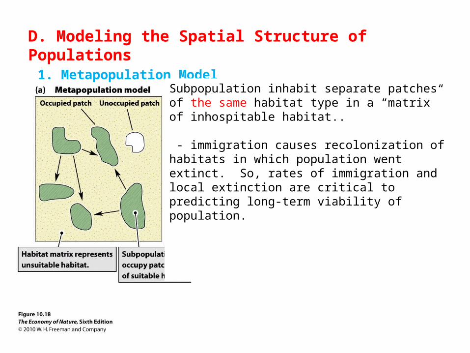
D. Modeling the Spatial Structure of Populations 2. Source-Sink Model
Subpopulation inhabit patches of different habitat quality, so there are ‘source’ populations with surplus populations that disperse to populations in lower quality patches (‘sinks’).

D. Modeling the Spatial Structure of Populations 3. Landscape Model
Subpopulation inhabit patches of different habitat quality, so there are ‘source’ populations with surplus populations that disperse to populations in lower quality patches (‘sinks’). However, the quality of the patches is ALSO affected by the surrounding matrix… alternative resources, predators, etc. And, the rate of migration between patches is also affected by the matrix between patches… with some areas acting as favorable ‘corridors’

E. Macroecology 1. Some General Patterns - Species with high density in center of range often have large ranges
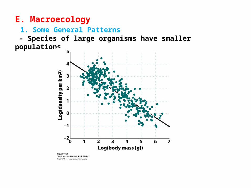
E. Macroecology 1. Some General Patterns - Species of large organisms have smaller populations
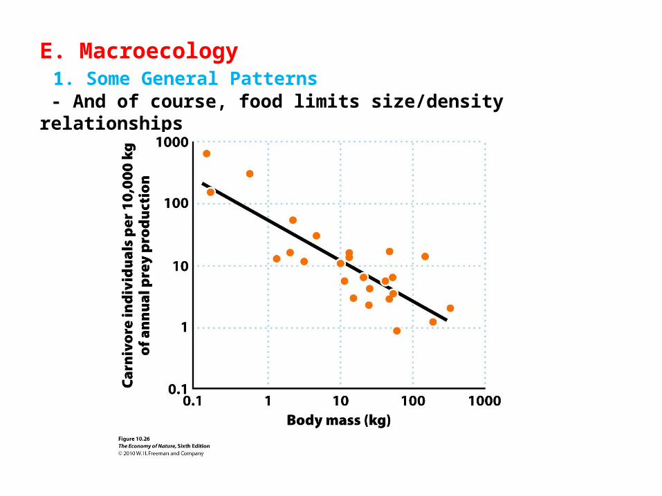
E. Macroecology 1. Some General Patterns - And of course, food limits size/density relationships
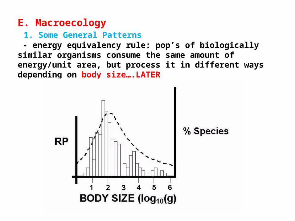
E. Macroecology 1. Some General Patterns - energy equivalency rule: pop’s of biologically similar organisms consume the same amount of energy/unit area, but process it in different ways depending on body size….LATER

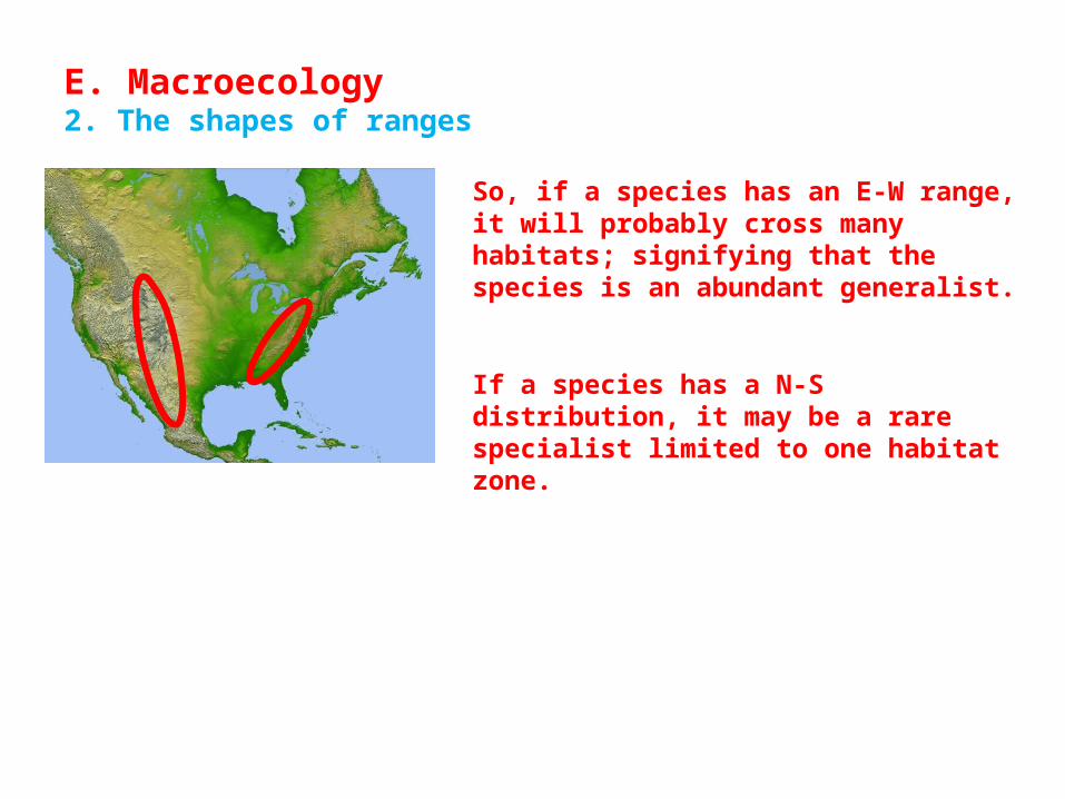
E. Macroecology2. The shapes of ranges - Abundant species have ranges running E-W; rare species have N-S ranges
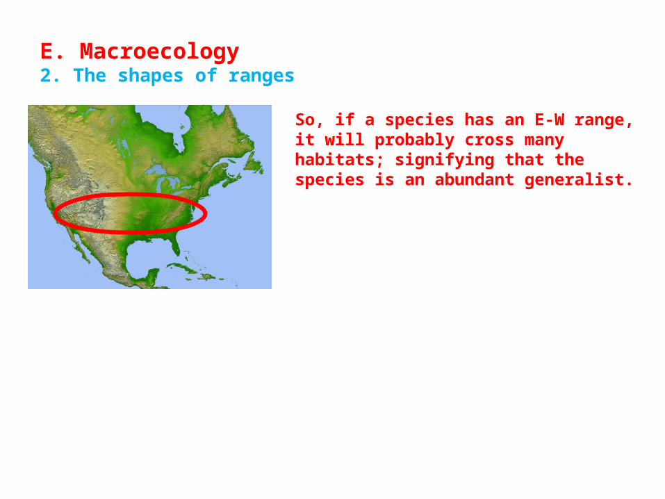
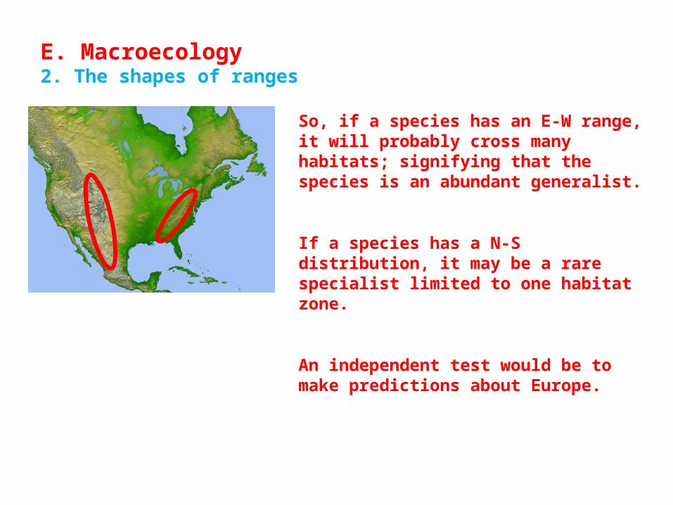
So, if a species has an E-W range, it will probably cross many habitats; signifying that the species is an abundant generalist.
E. Macroecology2. The shapes of ranges
So, if a species has an E-W range, it will probably cross many habitats; signifying that the species is an abundant generalist.
If a species has a N-S distribution, it may be a rare specialist limited to one habitat zone.
E. Macroecology2. The shapes of ranges
So, if a species has an E-W range, it will probably cross many habitats; signifying that the species is an abundant generalist.
If a species has a N-S distribution, it may be a rare specialist limited to one habitat zone.
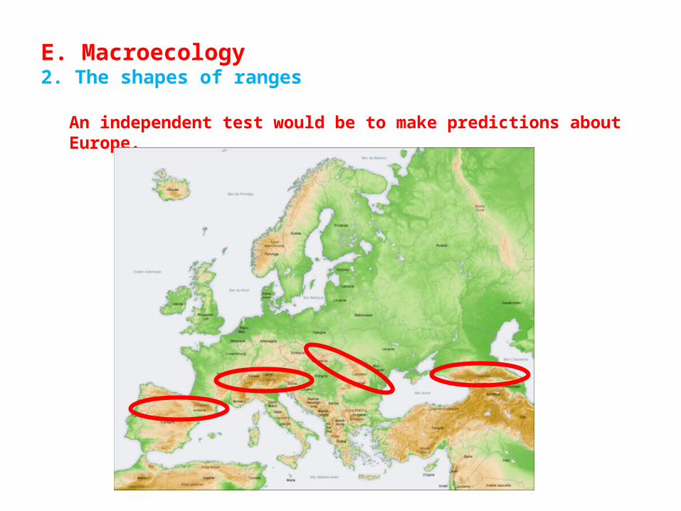
An independent test would be to make predictions about Europe.
E. Macroecology2. The shapes of ranges
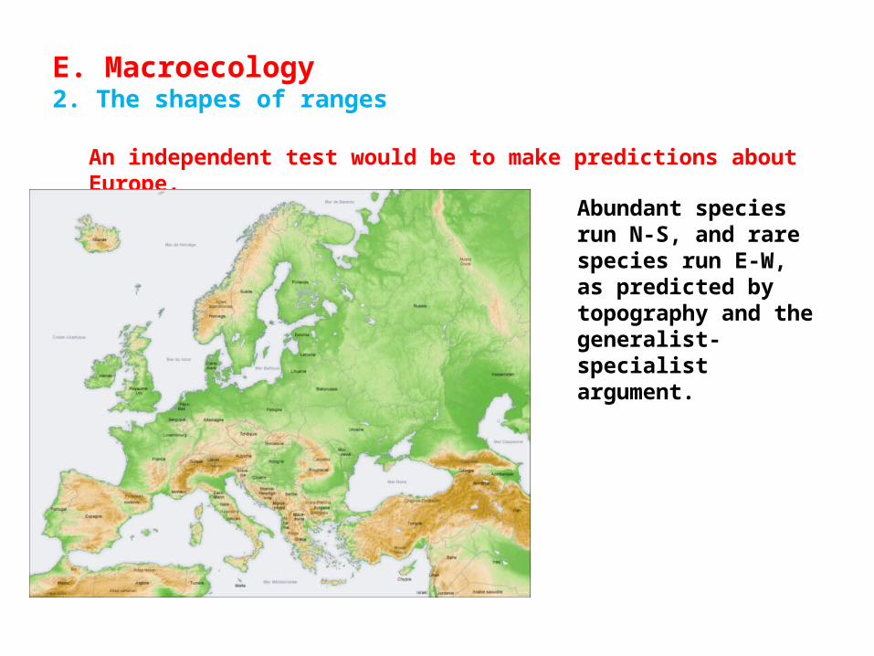
An independent test would be to make predictions about Europe.
E. Macroecology2. The shapes of ranges
An independent test would be to make predictions about Europe.
Abundant species run N-S, and rare species run E-W, as predicted by topography and the generalist-specialist argument.
E. Macroecology2. The shapes of ranges

Population EcologyI.Attributes of PopulationsII.DistributionsIII. Population Growth – change in size through time
A. Calculating Growth Rates1. Geometric Growth
Population EcologyI.Attributes of PopulationsII.DistributionsIII. Population Growth – change in size through time
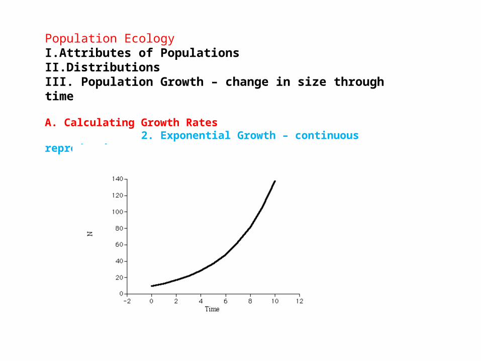
A. Calculating Growth Rates2. Exponential Growth – continuous reproduction

Population EcologyI.Attributes of PopulationsII.DistributionsIII. Population Growth – change in size through time
A. Calculating Growth Rates3. Equivalency
III. Population Growth – change in size through timeA. Calculating Growth Rates
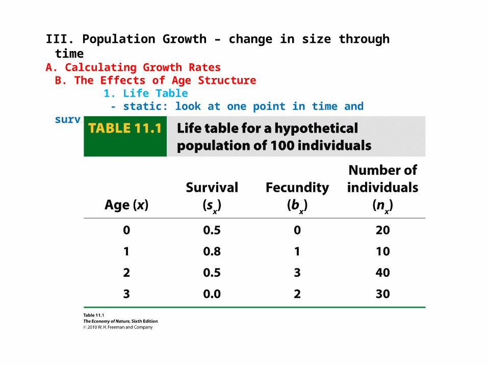
B. The Effects of Age Structure1. Life Table - static: look at one point in time and survival for one time period
III. Population Growth – change in size through timeA. Calculating Growth Rates
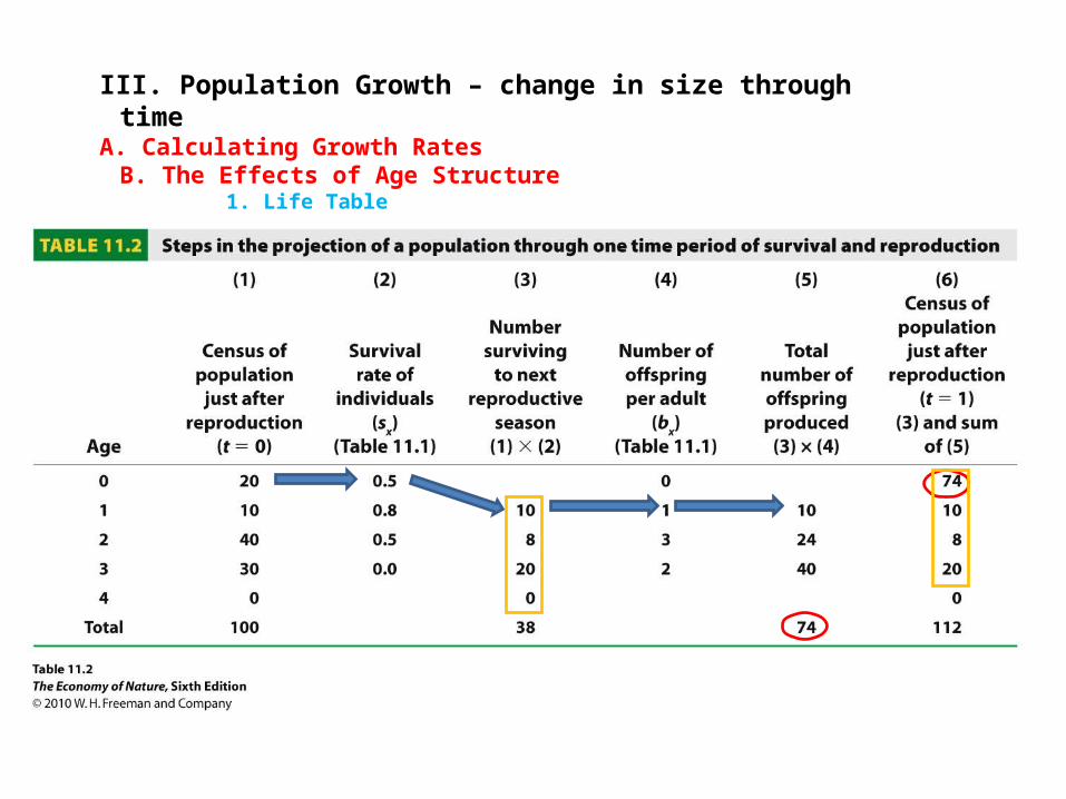
B. The Effects of Age Structure1. Life Table

III. Population Growth – change in size through timeA. Calculating Growth Rates
B. The Effects of Age Structure1. Life Table
Why λ ?
III. Population Growth – change in size through timeA. Calculating Growth Rates
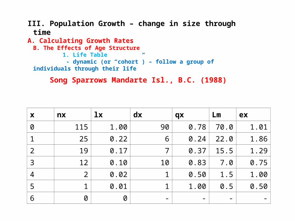
B. The Effects of Age Structure1. Life Table - dynamic (or “cohort”) – follow a group of individuals through
their life
x nx lx dx qx Lm ex
0 115 1.00 90 0.78 70.0 1.01
1 25 0.22 6 0.24 22.0 1.86
2 19 0.17 7 0.37 15.5 1.29
3 12 0.10 10 0.83 7.0 0.75
4 2 0.02 1 0.50 1.5 1.00
5 1 0.01 1 1.00 0.5 0.50
6 0 0 - - - -
Song Sparrows Mandarte Isl., B.C. (1988)

Age classes (x): x = 0, x = 1, etc. Initial size of the population: nx, at x = 0.
x nx lx dx qx Lm ex
0 115
1
2
3
4
5
6

Age classes (x): x = 0, x = 1, etc. Initial size of the population: nx, at x = 0. Number reaching each birthday are subsequent values of nx
x nx lx dx qx Lm ex
0 115
1 25
2 19
3 12
4 2
5 1
6 0
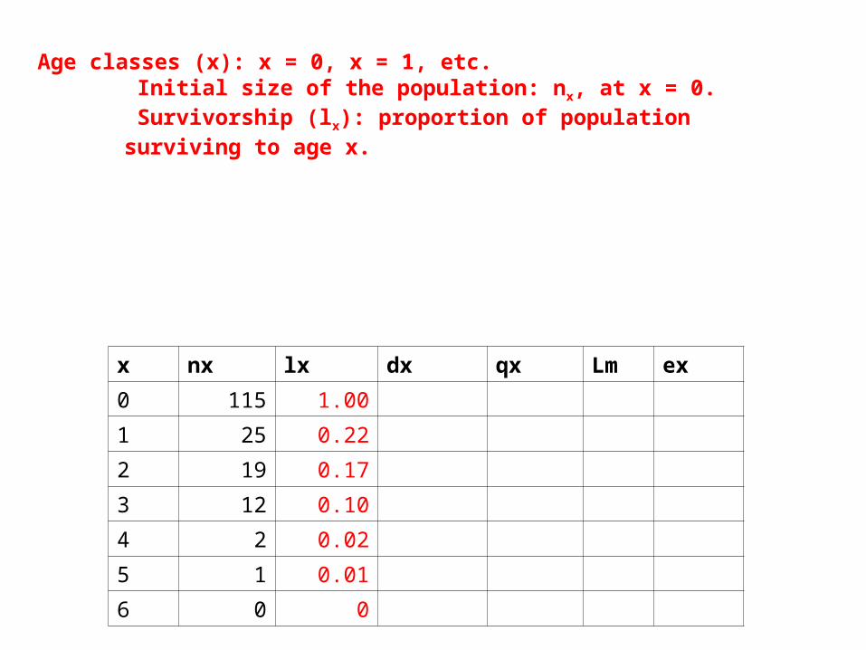
Age classes (x): x = 0, x = 1, etc. Initial size of the population: nx, at x = 0. Survivorship (lx): proportion of population surviving to age x.
x nx lx dx qx Lm ex
0 115 1.00
1 25 0.22
2 19 0.17
3 12 0.10
4 2 0.02
5 1 0.01
6 0 0
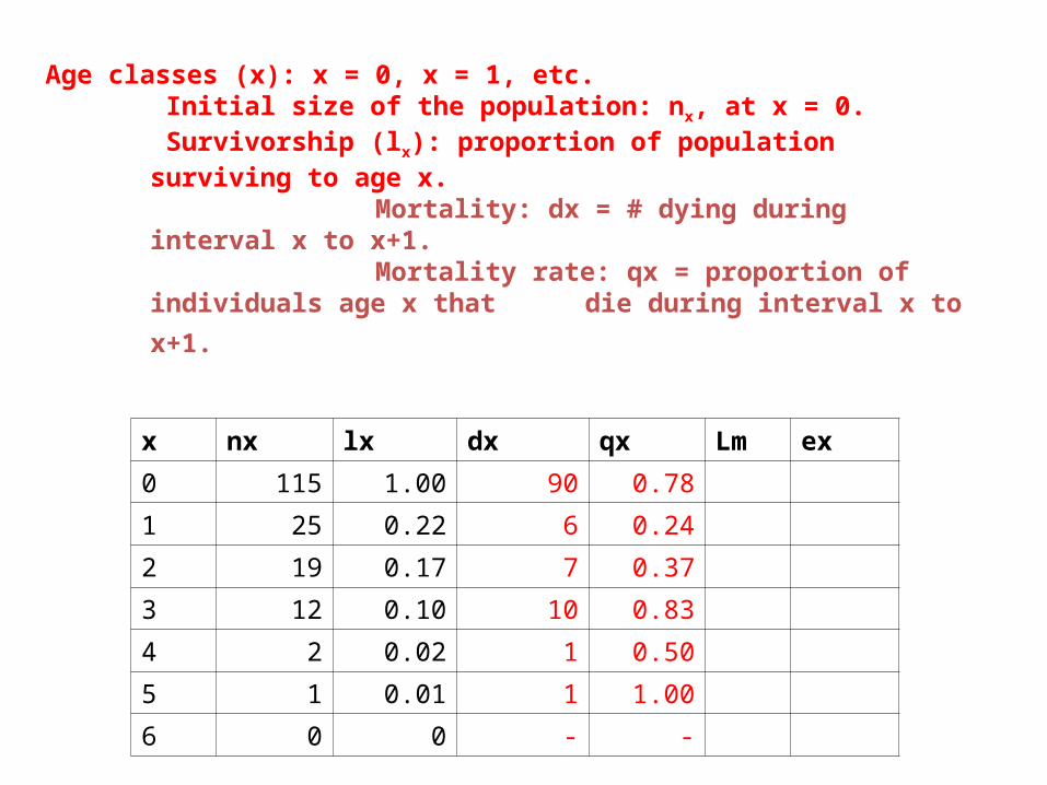
Age classes (x): x = 0, x = 1, etc. Initial size of the population: nx, at x = 0. Survivorship (lx): proportion of population surviving to age x. Mortality: dx = # dying during interval x to x+1.
Mortality rate: qx = proportion of individuals age
x that die during interval x to x+1.
x nx lx dx qx Lm ex
0 115 1.00 90 0.78
1 25 0.22 6 0.24
2 19 0.17 7 0.37
3 12 0.10 10 0.83
4 2 0.02 1 0.50
5 1 0.01 1 1.00
6 0 0 - -

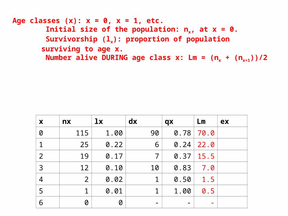
Age classes (x): x = 0, x = 1, etc. Initial size of the population: nx, at x = 0. Survivorship (lx): proportion of population surviving to age x. Number alive DURING age class x: Lm = (nx + (nx+1))/2
x nx lx dx qx Lm ex
0 115 1.00 90 0.78 70.0
1 25 0.22 6 0.24 22.0
2 19 0.17 7 0.37 15.5
3 12 0.10 10 0.83 7.0
4 2 0.02 1 0.50 1.5
5 1 0.01 1 1.00 0.5
6 0 0 - - -
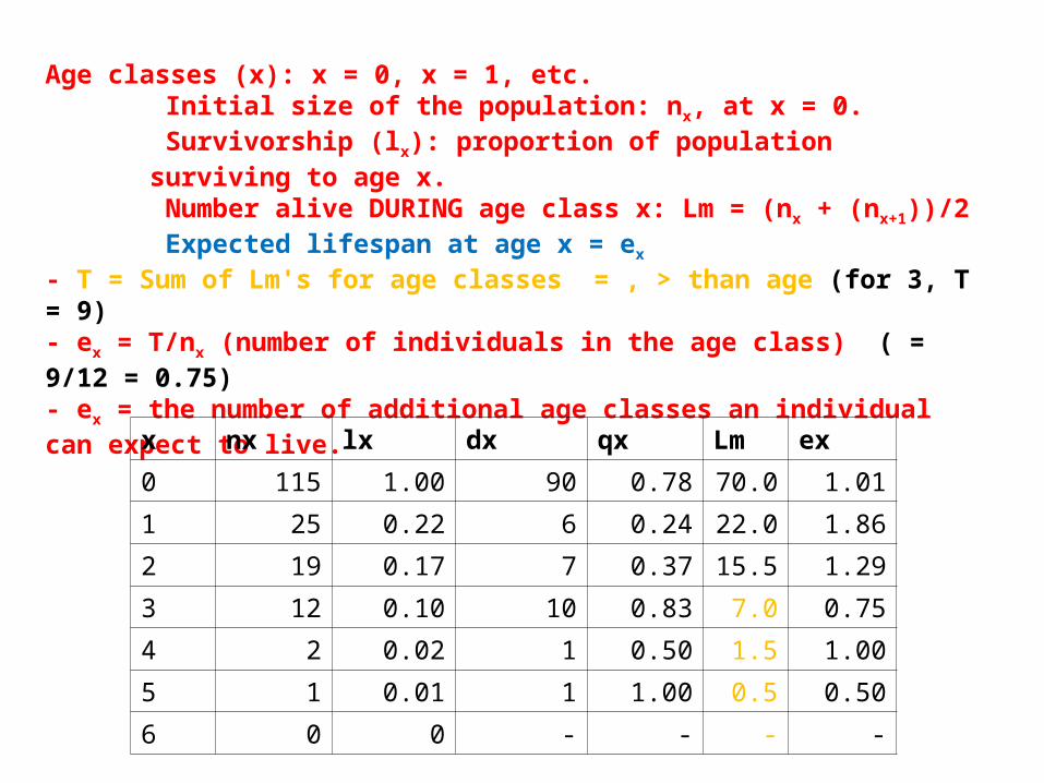
Age classes (x): x = 0, x = 1, etc. Initial size of the population: nx, at x = 0. Survivorship (lx): proportion of population surviving to age x. Number alive DURING age class x: Lm = (nx + (nx+1))/2 Expected lifespan at age x = ex
- T = Sum of Lm's for age classes = , > than age (for 3, T = 9)- ex = T/nx (number of individuals in the age class) ( = 9/12 = 0.75)- ex = the number of additional age classes an individual can expect to live.
x nx lx dx qx Lm ex
0 115 1.00 90 0.78 70.0 1.01
1 25 0.22 6 0.24 22.0 1.86
2 19 0.17 7 0.37 15.5 1.29
3 12 0.10 10 0.83 7.0 0.75
4 2 0.02 1 0.50 1.5 1.00
5 1 0.01 1 1.00 0.5 0.50
6 0 0 - - - -

III. Population Growth – change in size through timeA. Calculating Growth Rates
B. The Effects of Age Structure1. Life Tables2. Age Class Distributions
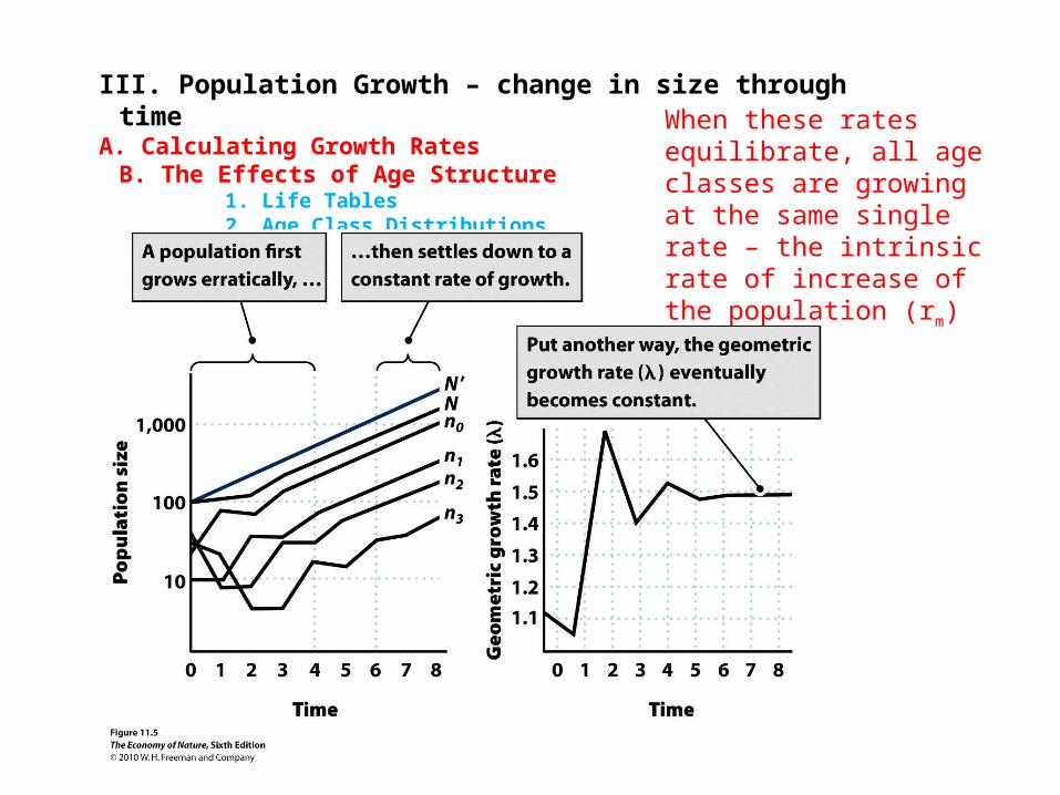
III. Population Growth – change in size through timeA. Calculating Growth Rates
B. The Effects of Age Structure1. Life Tables2. Age Class Distributions
When these rates equilibrate, all age classes are growing at the same single rate – the intrinsic rate of increase of the population (rm)
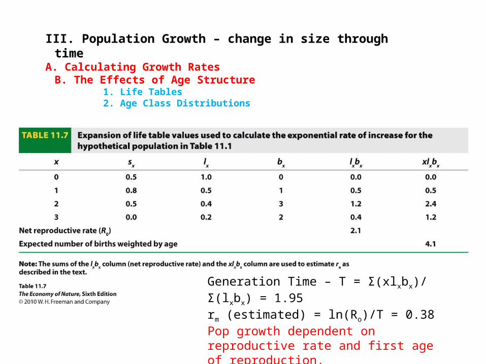
III. Population Growth – change in size through timeA. Calculating Growth Rates
B. The Effects of Age Structure1. Life Tables2. Age Class Distributions
Generation Time – T = Σ(xlxbx)/ Σ(lxbx) = 1.95rm (estimated) = ln(Ro)/T = 0.38Pop growth dependent on reproductive rate and first age of reproduction.Doubling time = t2 = ln(2)/r = 0.69/r