KANT AND LINDAHL

By

John E. Roemer and Joaquim Silvestre

February 2021

COWLES FOUNDATION DISCUSSION PAPER NO. 2278

COWLES FOUNDATION FOR RESEARCH IN ECONOMICS YALE UNIVERSITY

Box 208281 New Haven, Connecticut 06520-8281

http://cowles.yale.edu/

“Kant and Lindahl”

by John E. Roemer, Yale University,

and Joaquim Silvestre, University of California, Davis*

February 2021

1. Introduction

A good is public if its consumption is nonrival, and some public goods are nonexcludable. We

consider three different ways by which the amounts of a public good and the distribution of its costs

are determined: (i) The political system; (ii) Private supply by voluntary contributions; (iii) The

supply of an excludable public good by private firms.

1.1. Public provision by the political system

For many public goods, the decisions on their provision and financing are made by the public

sector. These goods are quantitatively important, their supply requiring a substantial fraction of the

budget at all levels of government. Knut Wicksell (1896) and Erik Lindahl (1919) analyzed the

operation of a representative parliament.1 They envisaged a negotiation among the various parties in

the parliament until all universally beneficial alternatives were exhausted. The resulting unanimous

agreement yields (Pareto) efficiency. Section 2 below offers a precise model.

1.2. Private provision by voluntary contributions

Some public goods are provided outside the public sector and outside the market by

individual voluntary contributions: the textbook example is public radio. These tend to be

quantitatively less important than the ones provided by the government. But information is a

public good par excellence: thanks to the internet, much information is now provided on a

voluntary contribution basis (Wikipedia, consumer ratings of products…).

The voluntary provision of public goods is most naturally formalized as a game in normal

formal, where each player chooses her individual strategy, namely her contribution. The early

analysis (Mancur Olson, 1965, see Theodore Bergstrom, Lawrence Blume and Hal Varian, 1986,

* We are deeply indebted to Andreu Mas-Colell for useful comments and suggestions, with the usual caveat. 1 See Silvestre (2003) for a discussion.

2

and the references therein) adopted the Cournot-Nash equilibrium concept, and emphasized its

typical inefficiency, the “free rider problem,” which reflects the absence of cooperation.

In contrast, Roemer (2010, 2019) offers a cooperative approach to normal-form games. It is

based on an alternative behavioral assumption or optimization protocol inspired by Immanuel

Kant’s (1758) categorical imperative (sections 3 and 5 below). The resulting equilibrium

allocations are efficient.

1.3. Private provision by the market

If an individual can be prevented from accessing an existing public good, then it is possible

to finance its supply by access prices or user fees. In our internet age, with encrypted passwords, it is

cheap for a supplier to deny access to software, networks, news, satellite TV, Google, and all sorts of

information. Hence, significant public goods are now provided by privately owned, profit

maximizing firms. (Section 6 below.)

Some of the issues concerning these markets are studied in the economics of public utilities.2

Duncan Foley (1970) (see also Françoise Fabre-Sender, 1969, and John Roberts, 1974) reformulated

the insights of Lindahl (1919) eliminating the public sector and the political parties and envisioning

instead a pseudo-Walrasian equilibrium where the public good is traded by price-taking buyers and

sellers. The equilibrium is then blessed with efficiency by the Invisible Hand.

1.4. Our analysis

We see that three of these models (Wicksell-Lindahl, Kant, and Foley) yield efficiency. In

addition, there are formal parallelisms among them. The relationship between Wicksell-Lindahl and

Foley has been provided, e. g., by Andreu Mas-Colell and Silvestre (1989): see Fact 6.1 below. The

present paper focuses on the relationship between the Wicksell-Lindahl and Kantian models.

We emphasize the fundamental difference between these two worlds. In Wicksell and

Lindahl, the public sector deliberates and decides, in a centralized way, on the supply of the public

goods and on their financing: this is the world of national defense. In Roemer’s Kantian approach,

each person separately decides how much to contribute towards the financing of the public good:

this is the world of public radio. Both models display efficiency. Moreover, the primary versions of

either model are defined by the same individual optimization problem (Section 4.1 below) and,

2 See Silvestre (2012, Ch. 5)

3

under differentiability, a person’s cost share equals her Lindahl Ratio (i. e., her marginal valuation of

the public good divided by the social marginal valuation: Section 4.2 below); in other versions, a

person’s cost share departs from her Lindahl ratio in ways made precise in sections 5 and 6 below.

1.5. The economy

We consider a society with one private, desirable, non-produced good, and M produced

public goods. A vector of public goods is denoted . The social technology is

defined by a cost function , where C(y) is the amount of the private good required to

produce the vector y of public goods.

There are N persons in society. Person i is endowed with units of the private good and a

utility function ui(xi, y), strictly increasing in xi, Person i’s consumption of the private good.

A state of the economy is a vector (x, y) = (x1,…, xN; y1,…,yM) .

Definition 1.1. A state (x, y) is feasible if .

Definition 1.2. A feasible state (x, y) is efficient if there is no other feasible state which gives

every person a weakly greater utility, and some person a greater utility.

2. The political system: Wicksell and Lindahl

Wicksell (1896 [1958, pp. 89-90]) states:

“ As long as the project in question permits the creation of utility beyond its cost, it would always be theoretically possible, and often feasible in practice, to find a cost-sharing scheme such that all parties consider the project beneficial, so that their unanimous approval would be possible.”

The Wicksellian view is thus centralized: the parties in the parliament negotiate and find a

cost-share scheme at which they unanimously agree on the vector of public goods. The idea of

unanimity based on a cost-sharing scheme motivates the analyses by Mamoru Kaneko (1977, see

Definition 7.3 below) and Mas-Colell and Silvestre (1989). We adapt the following definition from

the latter.

Definition 2.1. A cost share system is a family of N functions , i = 1,…., N,

such that for all y.

y = (y1, y2,..., yM )∈ℜ+M

C :ℜ+M →ℜ+

ω i

∈ℜ+N+M

C(y) ≤ [ω ii=1

N∑ − xi ]

gi :ℜ+M →ℜ

gii=1

N∑ (y) = C(y)

4

Definition 2.2. A Cost Share Equilibrium is a pair comprising a state (x*, y*) and a cost share

system (g1, …, gN) such that, for i = 1,…, N:

(i) xi* = ;

(ii) ui(xi*, y*) > , for all .

We then say that state (x*, y*) is supported by a Cost Share Equilibrium. We shall use the

terms “supported” and “supportable” for any equilibrium concept.

Fact 2.1. It is shown in Proposition 1 of Mas-Colell and Silvestre (1989) that a Cost Share

Equilibrium is efficient. The only assumption required is the above-mentioned increasingness of

utility with respect to the private good.

Lindahl’s (1919) formal discussion, presented in his doctoral thesis written under Wicksell’s

direction, considers two representative parties (for the rich and the poor), but he notes that the

analysis can be extended to any number of parties.3 Our discussion here admits an arbitrary number

of parties. It is convenient to visualize all the constituents of a given party as having exactly the

same interests, so that the preferences of Party i are truly representative of the interests of its

constituents.4 For convenience of comparison within sections, here we use the notation N for the

number of parties (realistically, a few) rather than the number of individuals (some millions).

Lindahl (1919) specializes Wicksell’s view in a formally explicit model that appeals to

proportionality or linearity. In his words, (Lindahl, 1919 [1958, p. 173]): “collective goods do not

have the same order of priority for all,” in which case “each party must undertake to pay a greater

share than the other toward the cost of these services which each finds most useful.” This motivates

the following definition (Mas-Colell and Silvestre, 1989). Here and in what follows we denote by

the (N - 1)-dimensional standard simplex.

Definition 2.3. A cost share system is linear if it is of the form gi(y) = , i

= 1,…, N, satisfying

; (2.1)

3 Thomas Piketty (2019, pp. 226-231) describes the Swedish society of the 19th century as extremely unequal and “quaternary,” with four groups represented in the riksdag (parliament). 4 The cost share of an individual will then be the cost share of her party divided by the number of constituents, see Silvestre (2012, Section 4.3.1).

ω i − gi (y*)

ui (ω i − gi (y), y) y ∈ℜ+M

ΔN−1 ≡ {(α1,...,αN )∈ℜ+N : α ii=1

N∑ = 1}

aij

j=1

M∑ y j + biC(y)

(b1,...,bN )∈ΔN−1

5

For j = 1,…, M, . (2.2)

Definition 2.4. A Linear Cost Share Equilibrium (LCSE) is a Cost Share Equilibrium for a

linear cost share system.

It follows from (2.2) that , i. e. , represents a

net transfer from (or to) Person i, the aggregate net transfer being zero. We can interpret a Linear

Cost Share Equilibrium as distributionally impartial if every individual transfer is zero, leading to

the following definition.

Definition 2.5. A Linear Cost-Share Equilibrium is Balanced (a BLCSE) if, for i = 1,…, N,

= 0.

Remark 2.1. Balanced Linear Cost Share Equilibria exist under convexity, as long as the

private good is indispensable and nobody considers the public good a bad (Mas-Colell and

Silvestre, 1989, Proposition 7). These equilibria may or may not exist under increasing returns to

scale: it may depend upon the relative curvatures of the cost and indifference curves. Theorems

4.1-2 below prove existence under increasing returns to scale in a special case.

3. Kantian decentralized cooperation and the voluntary provision of public goods

3.1. Simple and Multiplicative Kantian Equilibria in abstract games

The Cournot-Nash model has become the canonical paradigm for the theory of human

interaction in modern economics. Formally, a normal-form game is defined by a list i = 1,…,N

of players, and, for i = 1,…, N, a strategy set Ii and a payoff function . In the

Cournot-Nash approach, Player i chooses the strategy that is best for her while taking as given

the strategies played by other players. The resulting equilibrium is typically inefficient,

evidencing the noncooperative character of the Cournot-Nash Equilibrium.

But humans do cooperate (Roemer, 2019, Ch. 1). There are two approaches to including

cooperation within the Cournot-Nash paradigm. First, one may design complex games with an

indefinite number of stages where efficient outcomes are enforced by punishments (Michihiro

Kandori, 1992). A second approach is to assume that the payoff functions involve altruism or a

preference for socially efficient outcomes.

aij

i=1

N∑ = 0

y j aij

i=1

N∑j=1

M∑ = aij

j=1

M∑ y ji=1

N∑ = 0 aij

j=1

M∑ y j

aij

j=1

M∑ y j

Vi : Ihh=1

N∏ →ℜ

6

Roemer’s Kantian approach maintains the modelling of a normal-form game but

repudiates the Cournot-Nash behavioral assumption in all its forms. Instead, it bases cooperation

on the desire to do “the right thing” in a version of Kant’s categorical imperative. This leads to

the following notions (Roemer 2010, 2019).

Definition 3.1. Let be a normal form game satisfying

. A Simple Kantian Equilibrium is a strategy satisfying, for i = 1,… , N,

.

Simple Kantian Equilibria (usually) exist when the game is symmetric (i. e., there is a

function such that for all i, where ), as in the Prisoner’s

Dilemma. They may or may not exist when the set I is discrete. They typically fail to exist when

Ii is an interval of real numbers, which we assume in what follows, and players have different

payoff functions. (Simple Kantian Equilibria do exist with identical players, see Theorem 4.2

below.) But Kantian equilibria according to the following definition often exist. Other “kinds of

action” are described in Section 5.2 below.

Definition 3.2. Let Ii be an interval of real numbers, i = 1,…, N. A strategy profile

is a Multiplicative Kantian Equilibrium if, for i = 1, …, N, solves

subject to .

In words, no player would like to re-scale the whole vector of strategies.

3.2. Simple and Multiplicative Kantian Equilibria for the voluntary contribution

game

Many of our points are most clearly expressed in a model with a single public good.

Accordingly, we focus on the case M = 1 in sections 3-6 here and below. We suppress the

superindices in the notation of sections 1.5 and 2 above. We take the cost function

to be strictly increasing, and, hence, invertible.

Definition 3.3. The Voluntary Contribution Game is the game in normal form where, for

, Player i’s strategy is and her payoff function is

.

The Cournot-Nash equilibria of this game are typically inefficient (free rider problem).

((1,...,N ),(I1,..., IN ),(V1,...,VN ))

Ii = I ,∀i t* ∈I

Vi (t*,...,t*) ≥Vi (t,...,t),∀t ∈I

V Vi (t1,...,tN ) = V (ti ,tS\i ), tS\i = thh≠i∑

(t1,...,tN ) ρ = 1

maxρ≥0 Vi (ρt1,...,ρtN ) ρti ∈Ii

C :ℜ+ →ℜ+

i = 1,...,N ti ∈[0,ω i ]≡ Ii

Vi (t1,...,tN ) = ui (ω i − ti ,(C)−1( thh=1

N∑ ))

7

Definitions 3.1 and 3.2 can be applied to the Voluntary Contribution Game as follows.

Definition 3.4. The vector is a Simple Kantian Equilibrium

(SKE) for M = 1 if, for i = 1,…, N,

(i). , ;

(ii). solves max subject to , . (3.1)

Definition 3.5. A Multiplicative Kantian Equilibrium (MKE) for M = 1 is a vector

such that, for i = 1,…, N , solves

subject to ,

with and .

In words, no person would like to transform the vector into the vector

with the corresponding change in the level of the public good.5

4. Balanced Cost Share Equilibria and Simple or Multiplicative Kantian Equilibria

4.1. Equivalence results

Our next definition specializes definitions 2.1-5 above.

Definition 4.1. A Balanced Linear Cost Share Equilibrium (BLCSE) for M = 1 is a state

and a vector such that, writing ,

solves max subject to , i = 1,…, N. (4.1)

Because , , i. e., . Hence, as long as , (4.1)

can be written: max subject to . (4.2)

Theorem 4.1. Equivalence result for Simple Kantian Equilibria. Let M = 1.

is a Simple Kantian Equilibrium if and only if is a Balanced

Linear Cost Share Equilibrium with

5 A related idea appears in Silvestre (1984) .

((x*, y*),(t1*,...,tN

* )∈ℜ+N+1+N

ti* = t* ∈[0,ω i ] xi

* = ω i − t*

(t*, y*) ui (ω i − ti , y) y = C−1(Nti ) ti ∈[0,ω i ]

((x*, y*),(t1*,...,tN

* ))∈ℜ+N+1+N ρ = 1

maxρ∈ℜ+ui (ω i − ρti

*,(C−1)(ρ th*

h=1

N∑ )) ω i − ρti* ∈[0,ω i ]

y* = (C−1)( th*

h=1

N∑ ) xi* = ω i − ti

*

(t1*,...,tN

* )

(ρt1*,...,ρtN

* )

(x*, y*)∈ℜ+N+1 (b1,...,bN )∈ΔN−1 ti

* = ω i − xi*

(ti*, y*) ui (ω i − ti , y) ti = biC(y)

bhh=1

N∑ = 1 th*

h=1

N∑ = C(y*) ti* = bi th

*h=1

N∑ y* > 0

ui (ω i − ti , y) ti = ti*

th*

h=1

N∑C(y)

((x*, y*),(t1*,...,tN

* ))∈ℜ+N+1+N (x*, y*)

bi = 1N

,i = 1,...,N .

8

Proof. In a BLCSE with bi = 1/N, we have [by (4.1)] that maximizes

subject to .It follows that , and hence

solves max subject to . (4.3).

But this defines, by (3.3), a SKE: the objective function is the same in (3.1) and (4.3), and so is the

constraint, because . ∎

As noted in Section 3, Simple Kantian Equilibria typically fail to exist. We next show

that they do in the special case where all N persons are identical.

Assumption 4.1. Identical persons. Let M = 1, , and let the utility function be

the same for , i. e., .

Theorem 4.2. Assume M = 1 and identical persons. If u and C are continuous, and C is

unbounded, then a Simple Kantian Equilibrium exists.

Proof. Because C is unbounded, continuous and increasing, C and C-1 are defined and

continuous on . Thus, the function is continuous on the compact

interval . ∎

Consider Figure 4.1. The equilibrium, identical for all i, is found by maximizing

on the (thick) constraint curve. When reading the result with y as an independent

variable, it is Cost-Share. When read with ti as an independent variable it is Kant. In words,

everybody is treated equally in terms of contributions: in one case (Cost-Share) by the imposition

of equal cost shares; in the other by an internalized moral hypothesis (Kant). But then the result

of the optimization must be the same.

We can further simplify the illustration letting C(y) = y (constant returns to scale). Then

the thick curve in Figure 4.1 becomes the straight line " ” or " .” Cost Share goes

from y to by dividing, while Kant goes from to y by multiplying.

We now exit the identical person case: Simple Kantian Equilibria typically fail to exist

when people have different endowments or preferences. Consider a Multiplicative Kantian

(ti*, y*) ui (ω i − ti , y)

ti = 1N

C(y) ti* = 1

NC(y*) ≡ t*

(t*, y*) ui (ω i − ti , y) ti = 1N

C(y)

y = C−1(Nt)⇔ C(y)N

= t

ω i ≡ ω,∀i

∀i ui ≡ u :ℜ+2 →ℜ,i = 1,...,N

ℜ+ ψ(t) ≡ u(ω − t,(C−1)(Nt))

[0,ω]

u(ω − ti , y)

y = Nti ti = yN

ti ti

9

Equilibrium of Definition 3.5 above satisfying . We can then write and

reword Definition 3.5 as follows.

Definition 4.2. A Multiplicative Kantian Equilibrium for M = 1 with strictly positive

contributions is a vector such that, for i = 1,…, N , solves,

max subject to , , (4.4)

with and .

Theorem 4.3. Equivalence result for Multiplicative Kantian Equilibria. Let M = 1;

is a Multiplicative Kantian Equilibrium if and only if is a

Balanced Linear Cost Share Equilibrium with

Proof. The proof parallels that of Theorem 4.2 by appealing to the optimization problems

given by (4.2) for the BLCSE and (4.4) for the MKE. Again, their objective functions are the

same, and so are their constraints, since

. ∎

Figure 4.2 illustrates.Again, when reading the result with y as an independent variable it

is Cost-Share. When read with ti as an independent variable it is Kant.

Remark 4.1. Theorem 4.3 generalizes Theorem 4 in Roemer (2010).

Remark 4.2. Note that Theorem 4.2 does not require convexity (or differentiability).

Thus, Kantian Equilibria and Cost Share Equilibria are not incompatible with increasing returns:

see Remark 2.1. By Fact 2.1, they are all efficient: this contrasts with the Cournot-Nash

equilibria, typically inefficient even when all persons are identical (see, e. g., Silvestre, 2012,

Section 4.4.4).

4.2. The Lindahl Ratio

Assumption 4.2. Differentiability. The functions C and ui, i = 1, …, N, are differentiable.

The derivative C’, called the marginal cost and denoted m(y) or simply m, is assumed positive.

(t1*,...,tN

* )∈ℜ++N ρ = ti

ti*

((x*, y*),(t1*,...,tN

* ))∈ℜ+N+1 ×ℜ++

N (ti*, y*)

ui (ω i −ti

ti* ti

*, y) y = C−1 ti

ti* th

*h=1

N∑⎛⎝⎜

⎞⎠⎟

ti ∈[0,ω i ]

y* = (C)−1 th*

h=1

N∑( ) xi* = ω i − ti

*

((x*, y*),(t1*,...,tN

* ))∈ℜ+N+1 ×ℜ++

N (x*, y*)

bi = ω i − xi*

[ωh − xh* ]

h=1

N∑= ti

*

th*

h=1

N∑,i = 1,...,N .

y = C−1 ti

ti* th

*h=1

N∑⎛⎝⎜

⎞⎠⎟⇔ C(y) = ti

ti* th

*h=1

N∑ ⇔ ti = ti*

th*

h=1

N∑C(y)

10

We denote by i’s marginal rate of valuation of the public good. The

following fact is well known.

Fact 4.1. (Samuelson Condition). Assume differentiability and let the state be

efficient. Then .

Definition 4.3. Person i’s Lindahl Ratio at is , the ratio of

her marginal valuation of the public good to the social marginal valuation.

Theorem 4.4. Let M = 1. Assume differentiability. Let the state , with

, be supported by a Balanced Linear Cost Share Equilibrium or equivalently

(thanks to Theorem 4.3) by a Multiplicative Kantian Equilibrium. Then for i = 1,…, N, i’s relative

contribution towards the cost of the public good equals her Lindahl ratio, i. e.,

. (4.5)

Proof. The first order conditions of the (4.4) Lagrangean (we can equivalently use (4.2))

- ,

yield (4.5) , noting that and that

. ∎ (4.6)

By the equivalence between Multiplicative Kantian Equilibrium and Balanced Linear

Cost Share Equilibrium, either concept offers a theory of cost sharing. Here Kant meets Lindahl

in a strong way: your relative payment agrees with your relative marginal benefit, a version of

the “marginal benefit principle” which Lindahl defended normatively: see Section 8.1 below.

Remark 4.3. By the Samuelson Condition, , and hence the average Lindahl

Ratio is 1/N. Therefore, we will typically have for some i , whom we can call a

“High (Marginal) Valuator,” whereas for some h, a “Low (Marginal) Valuator.”

ri ≡∂ui

∂y∂ui

∂xi

(x, y)∈ℜ++N+1

rh (xhh=1

N∑ , y) = m(y)

(xi , y)∈ℜ++2 ri (xi , y)

m(y)≡ Li (xi , y)

(x*, y*)∈ℜ++N+1

ti* ≡ ω i − xi

* > 0,∀i

ω i − xi*

C(y*)≡ ti

*

C(y*)= Li (xi

*, y*)

ui (ω i −ti

ti* ti

*, y) λ y −C−1 ti

ti* th

*h=1

N∑⎛⎝⎜

⎞⎠⎟

⎡

⎣⎢

⎤

⎦⎥

(C−1 ′) = 1m

C(y*) = th*

h=1

N∑

Lhh=1

N∑ = 1

ti

C= Li > 1

N

th

C= Lh < 1

N

11

Remark 4.4. Under differentiability and interiority, Multiplicative Kantian Equilibria are

characterized by the system of 2N + 1 equations (4.5) (2N equations) and (4.6) in the 2N + 1

unknowns {xi}, {ti} and y. Hence, its solutions typically are locally unique and the set of states

supportable by a Multiplicative Kantian Equilibrium, or, equivalently, by a Balanced Linear Cost

Share Equilbrium, generically is a 0-dimensional manifold.

5. Additive and - Equilibria and their relation to Linear Cost Share Equilibria

5.1. The case of Constant Returns to Scale

Theorem 4.2 (resp., 4.1) above shows the equivalence between Balanced Linear Cost Share

Equilibria and Multiplicative Kantian equilibria (resp., Simple Kantian Equilibria, when they

exist). Despite their different rationales, these primary formulations of Kant’s and Lindahl’s ideas

are mathematically identical, and, as just noted in Remark 4.4, determinate.

We can consider broader versions of these equilibrium concepts which may in principle

support larger sets of states (all efficient). On Lindahl’s side, we can dispense with balancedness

and consider Linear Cost Share Equilibria (Definition 2.4 above). And on Kant’s side we can

contemplate a more general notions of “same kind of action” formalized as -Kantian or

equilibria (Roemer, 2019, and Section 5.2 below), and look at the set of states supported by such

equilibria as ranges over .

It turns out that the connection between these broader Lindahlian and Kantian notions loses

the simplicity of the primary notions in Section 4 above. We start with the special case of constant

returns to scale. We apply definitions 2.4-5 to the one-public-good case, and adopt the notation of

the first paragraph of Section 3.2.

Theorem 5.1. Let M = 1. Assume constant returns to scale, i. e., for some

, and that ui is nondecreasing in y, . The state is supported by a Linear

Cost Share Equilibrium if and only if it is supported by a Balanced Linear Cost Share

Equilibrium.

Proof. Trivially, a BLCSE is a LCSE. So let be supported by a LCSE with

parameters {ai}, {bi}, i. e., solves max ui(xi, y) s. to =

. Define, for i = 1,…, N, . Then the constraint is

K β

β K β

β [0,∞)

C(y) = my

m ∈ℜ++ ∀i (x*, y*)∈ℜ+N+1

(x*, y*)

∀i,(xi*, y*) xi = ω i − aiy − biC(y)

ω i − ai + bim[ ]y ai = 0,bi = ai

m+ bi xi = ω i − bimy

12

the same as in the original LCSE, and hence the solutions are the same. We are left with

checking that , satisfied since otherwise the original LCSE optimization would not have a

solution (because ui is nondecreasing in y), and that , satisfied because, by (2.1) and

(2.2), and . Thus . ∎

Remark 5.1. By Theorem 5.1, Linear Cost Share Equilibria do not expand, under constant

returns, the 0-dimensional set of states supported by Balanced Linear Cost Share Equilibria (see

Remark 4.4 above). Remarks 5.7 and 6.2 below offer some interpretation.

It follows from theorems 4.3 and 5.1 that, under constant returns to scale, a state is

supported by a Linear Cost Share Equilibrium if and only if it is supported by a Multiplicative

Kantian Equilibrium.

5.2. Additive and - Kantian Equilibria in abstract games

We follow Roemer (2019) and return to the abstract normal-form games of Section 3.1

above. We now postulate that the strategy set Ii is an interval of real numbers, i = 1,…, N.

Definition 5.1. A strategy profile is an Additive Kantian Equilibrium if, for i =

1, …, N, solves subject to .

Multiplicative and Additive Kantian optimization contemplate the set of counterfactuals

that every player considers to a given vector of strategies to be either all re-scalings of

that vector, or all translations of that vector, respectively. In both cases, all players contemplate

choosing a preferred counterfactual which lies in a common set of counterfactuals. This is in

contrast to the player who optimizes in the Nash manner: she contemplates choosing an altered

profile of strategies in which only her strategy changes, while the strategies of all other players

remain fixed. It is the consideration of a common set of counterfactuals which is the

mathematical expression of cooperation.

Finally, we can consider an optimization protocol where the set of counterfactuals – again

common to all – is generated by applying an affine transformation to the existing vector of

strategies. This gives the following equilibrium concept.

Definition 5.2. Given , define . A strategy profile is

a Kantian, or -, Equilibrium if, for i = 1, …, N, solves

bi ≥ 0

bhh=1

N∑ = 1

bhh=1

N∑ = 1 ahh=1

N∑ = 0 bhh=1

N∑ = 1m

ahh=1

N∑ + bhh=1

N∑ = 1

β

(t1,...,tN )

τ = 0 maxτ∈ℜVi (t1 + τ,...,tN + τ) ti + τ ∈Ii

(t1,...,tN )

β ≥ 0 ϕ(t,ρ) ≡ ρt +β[ρ−1] (t1,...,tN )

β − K β ρ = 1

13

subject to .

Remark 5.2. It immediately follows from definitions 3.1, 5.1 and 5.2 that a Simple Kantian

Equilibrium, when it exists, is an Additive Kantian Equilibrium and a -Equilibrium for any >

0. This in particular applies to the Identical Persons case of Theorem 4.2 above.

We now show that optimization comprises a continuum of possible optimization

protocols with additive and multiplicative Kantian optimization as its two endpoints:

Theorem 5.2. Suppose that the game in normal form is concave and continuously

differentiable, where the strategy spaces are closed intervals. Suppose, for sufficiently large

that is an interior - equilibrium of and that is a

limit point of as . Then is an Additive Kantian Equilibrium of .

Proof. By interiority and concavity, the first-order condition for to be a -

equilibrium is:

where is the gradient of evaluated at and 1 is the vector of 1’s in . Dividing

this equation by implies, as we let , that . But this is the necessary and

sufficient condition for to be an Additive Kantian Equilibrium of . Note that may

itself not be interior. The stated first-order condition for to be an additive Kantian equilibrium

is correct because is the limit of interior equilibria. ∎

Hence Multiplicative Kantian Equilbrium (the case ) and Additive Kantian

Equilibrium are the two poles of the continuum of equilibria.

Cooperation, defined as Kantian optimization, differs from altruism. Altruism is

represented by a consumption externality in preferences: an altruistic player values increasing the

utility or consumption of other players. Behavioral economists typically place ‘exotic’ arguments

in players’ preferences (e. g., the consumption of others), and then explain the apparently

altruistic or cooperative outcome of the game with altered preferences as Cournot-Nash

equilibria of that game. In contrast, the Kantian approach does not alter preferences from

maxρ∈ℜ+Vi (ϕ(t1,ρ),...,ϕ(tN ,ρ)) ϕ(ti ,ρ)∈Ii

K β β

K β

{Vi}

Ii

β ∈ℜ+ tβ = (t1β ,...,tN

β ) K β {Vi} t* = (t1*,...,tN

* )

{tβ} β→∞ t* {Vi}

tβ K β

∂Vi

∂thh=1

N

∑ (tβ )[th +β] = 0 = ∇Vi (tβ ) ⋅ tβ +β∇Vi (t

β ) ⋅1,

∇Vi (tβ ) Vi tβ ℜN

β β→∞ ∇Vi (t*) ⋅1 = 0

t* {Vi} t*

t*

t* K β

β = 0

K β

14

classical ones, but changes the optimization protocol. The cooperative morality, if you will, is

not displayed in preferences, but is represented in how people optimize.

The appellation ‘Kantian’ is derived from the ‘simple’ case: here, t is the strategy that

each player would like all players to play. In Immanuel Kant’s language, each player is taking

the action he ‘would will be universalized.’ The more general formulation is that all players

agree on a strategy profile to be chosen from a common set of profiles.

A game is strictly monotone increasing (decreasing) if each payoff function is a

strictly increasing (decreasing) function of the strategies of the players other than i. Strictly

increasing games are games with positive externalities, and strictly decreasing games are games

with negative externalities. The Voluntary Contribution Game of Definition 3.3 is monotone

increasing (as long as nobody dislikes the public good).

Fact 5.1. (Roemer, 2019). In any strictly monotone game, Simple Kantian Equilibria,

Additive Kantian equilibria, - Equilibria with , and Multiplicative Kantian Equilibria

with , are efficient.

Fact 5.1 justifies calling Kantian optimization a protocol of ‘cooperation,’ for it resolves

efficiently the free rider problem (in monotone increasing games) and the “tragedy of the

commons” (in monotone decreasing games, such as externality-causing activities) that

characterize Cournot-Nash optimization.

5.3. Additive and - Kantian Equilibria for the voluntary contributions game

Definitions 5.1-5.2 are adapted as follows.

Definition 5.3. An Additive Kantian Equilibrium for M = 1 is a vector

such that, for i = 1,…, N, solves

subject to ,

with and .

Definition 5.4. Let be given. A - Kantian, or -Equilibrium for M = 1 is a

vector such that, for i = 1,…, N , solves

subject to ,

Vi

K β β > 0

ti ∈IntIi ,∀i

β

((x, y),(t1,...,tN ))∈ℜ+N+1+N τ = 0

maxτ∈ℜ

ui (ω i − [ti + τ],(C−1)(Nτ + thh=1

N∑ )) ti + τ ∈[0,ω i ]

y = (C−1)( thh=1

N∑ ) xi = ω i − ti ,i = 1,...,N

β ∈ℜ+ β K β

((x, y),(t1,...,tN ))∈ℜ+N+1+N ρ = 1

maxρ∈ℜ+ui (ω i − [ρti +β[ρ−1]],(C−1)(Nβ[ρ−1]+ ρthh=1

N∑ )) ρti +β[ρ−1]∈[0,ω i ]

15

with , . (5.1)

By Theorem 4.3, and recalling Remark 2.1, Multiplicative Kantian Equilibria exist under

standard assumptions. The following theorem covers existence for .

Assumption 5.1. Convexity. The function C(y) is convex; the functions ui(xi ,y), i = 1,…,

N, are concave.

Theorem 5.3. Let M = 1. Assume convexity and continuity, and let ui(xi, y), i = 1, …, N,

be nondecreasing in y (nobody dislikes the public good).

(i). If , then a -Equilibrium exists.

(ii). An Additive Kantian (i. e., ) Equilibrium exists.

Proof. (i). Let be given. Write , and

. Given and , define the function

.

Because ui is concave and nondecreasing in (xi, y), and is linear in , and C -1 is concave, we

have that is a concave, continuous function of . Therefore, since , the set

is nonempty, compact and convex. Note that if , then , and

. By Berge’s Theorem, the correspondence that assigns

the set to a vector is bounded, upper hemicontinuous and convex

valued. Define the correspondence

.

In words, the best reply correspondence of Player i at a proposed vector of strategies

is to transform her strategy by the ‘factor’ that is ideal for i, restricting to values

that generate feasible strategies for Player i.

y = (C−1)( thh=1

N∑ ) xi = ω i − ti ,i = 1,...,N

β > 0

β > 0 K β

K ∞ −

β > 0 ϕ :ℜ+2 →ℜ :ϕ(t,ρ) = ρt +β[ρ−1]

Ω = [0,ω ii=1

N∏ ] (t1,...,tN )∈Ω i ∈{1,...,N}

ξi[t1,...,tN ] :ℜ+ →ℜ+ : ξi[t1,...,tN ](ρ) = ui (ω i −ϕ(ti ,ρ),C−1( ϕ(th ,ρ)h=1

N∑ ))

ϕ ρ

ξi[t1,...,tN ] ρ β > 0

ρi*(t1,...,tN ) ≡ argmax

βti +β

≤ρ≤ωi +βti +β

,

ui (ω i −ϕ(ti ,ρ),C−1( ϕ(th ,ρ)h=1

N∑ ))

ρi ∈ρi*(t1,...,tN ) ϕ(ti ,ρi )∈[0,ω i ]

βω i +β

≤ βti +β

≤ ρ ≤ ω i +βti +β

≤ ω i +ββ

ρi*

ρi*(t1,...,tN ) (t1,...,tN )∈Ω

Bi :Ω→→ [0,ω i ] : Bi (t1,...,tN ) = {!ti ∈[0,ω i ] : !ti = ϕ(ti ,ρi )for some ρi ∈ρi*(t1,...,tN )}

(t1,...,tN ) ρ ρ

16

Again because is linear in , the set Bi(t1,…, tN) inherits compactness and convexity

from the set , and the correspondence inherits upper hemicontinuity from the

correspondence .

Define the correspondence By

Kakutani’s Theorem has a fixed point , i. e., for i = 1,…, N,

. Since

, it follows that, for all i, such . So a fixed point is a - Equilibrium.

(ii). Adapt the argument in (i) by replacing by the set

.

At a fixed point , . Thus, a fixed point is an

Additive Kantian Equilibrium. ∎

Remark 5.3. Equilibria may involve corner solutions , for some i.

Remark 5.4. In Section 3.1, we contrasted Kantian equilibria in games to the typical

approach in behavioral economics to explaining non-classical Cournot-Nash equilibria in real

situations, which is defining preferences over non-standard arguments (e. g., other people’s

consumption or utility). Typically this is done in an experimental setting, where the game being

played is quite a simple one. Often, indeed, these experimental games are symmetric. Theorem

5.2, in contrast, tells us that, in the voluntary contribution game, Kantian equilibria exist for very

complex and heterogeneous preferences (assuming only they are continuous and convex). How

would one design exotic preferences whose Nash equilibrium would, in such a complex, altered

game, be Pareto efficient? Roemer (2019, Chapter 6) argues there is no acceptable way of

accomplishing this: the move of including exotic arguments in preferences is ad hoc and

insufficiently general.

Lemma 5.1. Let M = 1 and assume differentiablility and convexity, so that the first order

conditions are necessary and sufficient. The first order condition for an interior solution, i. e.,

, to i’s maximization problem, i = 1,…, N, are as follows.

For a -Equilibrium, (Definition 5.4):

ϕ ρ

ρi*(t1,...,tN ) Bi

ρi*

Φ :Ω→→Ω by Φ(t1,...,tN ) = (B1(t1,...,tN ),..., BN (t1,...,tN )).

Φ (t1*,...,tN

* )∈Ω

ti* = ρi [ti

* +β]−β, i.e., ti*[1− ρi ]+β[1− ρi ] = 0,for some ρi ∈ρi

*(t1*,...,tN

* )

β > 0 and ti* ≥ 0 ρi = 1 K β

ρi*(t1,...,tN )

τi*(t1,...,tN ) = argmax

− ti≤τ≤ωi−tiui (ω i − (ti + τ),C−1(tS + Nτ))

(t1*,...,tN

* ) ti* = ti

* + τi , i. e., τi = 0,i = 1,...,N

xi ∈{0,ω i}

ti ∈(0,ω i )

K β β ≥ 0

17

; (5.2)

For an Additive Kantian-Equilibrium (Definition 5.3) :

. (5.3)

Proof. Differentiate the relevant objective function and note that . ∎

We can rewrite (5.2) as , which if divided by C yields:

. (5.4)

Whenever , from (5.4) we obtain that:

* If i is a High Valuator (i. e., ), then: ,

* If h is a Low Valuator (i. e., ), then: .

In words, when > 0 a High (resp. Low) Valuator’s share in the cost is higher (resp.

less) than her Lindahl Ratio -- and also than the average share. Compare with Theorem 4.4

above, where (4.5) is (5.4) for = 0, and a person’s cost share is her Lindahl Ratio.

Remark 5.5. An interior - (resp. Additive Kantian) Equilibrium is determinate

(generically locally unique) in the sense that the equations defining it, namely the 2N + 1 equations

(5.1) & (5.2) (resp., (5.1) & (5.3)) in the 2N + 1 unknowns {ti},{xi} and y admit zero degrees of

freedom. To the extent that changes in change the equilibrium state, local uniqueness carries

over, and thus the set of states supportable by -equilibria as ranges over is 1-

dimensional. See the discussion at the end of Section 5.4.

What can we say about the - equilibria as becomes larger? Because, is

bounded, as long as all the solutions are interior, (5.2) yields 6

6 Equalities (5.3) and (5.5) illustrate the identification of a -Equilibrium with an Additive Kantian Equilibrium,

see Theorem 5.2. The identification of a -Equilibrium with a Multiplicative Kantian Equilibrium is displayed by (4.5) and (5.2).

Li ≡ri

m= ti +β

th + Nβh=1

N∑

Li ≡ri

m= 1

N

(C−1 ′) = 1′C= 1

m

ω i − xi = ti = Li[C + Nβ]−β

ω i − xi

C= ti

C= Li + βN

CLi −

1N

⎡⎣⎢

⎤⎦⎥

β > 0

Li > 1N

ω i − xi

C> Li

Lh < 1N

ωh − xh

C< Lh

β

β

K β

β

K β β [0,∞)

K β β ∀i, ti

K ∞

K 0

18

. (5.5)

Remark 5.6. Intuitively, high valuators pay more, hence they consume a smaller amount

of the private good, which typically increases its marginal utility, and hence decreases the

marginal rate of valuation . Conversely for low valuators. Of course, if the

marginal utility of the private good is not decreasing, as in the quasilinear case, then this process

does not work. Indeed, it may well happen that solutions are not interior, and (5.5) may fail. (See

also Remark 6.3 below.)

Even if (5.4) holds for all , we do not know how the RHS of (5.4) behaves as ,

since, by (5.5), its limit is indeterminate of the type . We have computed examples where

(5.4) holds for all but, as , converges to a limit other than .

5.4. Linear Cost Share Equilibria and -Kantian Equilibria

The constant-returns-to-scale case has been analyzed in Section 5.1. We now assume

differentiability, convexity and interiority in order to analyze the relationship between Linear

Cost Share Equilibria and - ( -Kantian ) Equilibria when my > C(y) (decreasing returns to

scale). Applying Definition 2.4 to the M = 1 case and appealing to the first-order conditions, an

interior Linear Cost Share Equilibrium is characterized by the following equalities:

(5.6)

. (5.7)

Remark 5.7. The set of states supportable as a Linear Cost Share Equilibrium under

constant returns to scale typically is 0-dimensional (Remark 5.1). Indeed, we can then collapse

equations (5.6) & (5.7) into the N equations: , which together with

constitute a determinate system of N + 1 equations in the N + 1 unknowns

(x, y). But for nonconstant returns to scale with , then, as argued in Mas-Colell and

Silvestre (1989), the 2N + 2 equations (5.6), (5.7), (2.1) and (2.2) in the 3N + 1 unknowns {xi},

{ai}, {bi} and y display N - 1 degrees of freedom, indicating that the set of states supportable as a

Linear Cost Share Equilibrium typically is (N - 1)-dimensional. See Remark 6.2 below.

limβ→∞

Li = 1N

ri (xi , y) ≡ ∂ui

∂y∂ui

∂xi

β β→∞

∞ i 0

β β→∞ ti

C1N

β

K β β

ai + bim = ri ,i = 1,...,N;

xi = ω i − aiy − biC(y),i = 1,...,N

xi = ω i − ri (xi , y)y,i = 1,...,N

[ω ih=1

N∑ − xi ] = my

C(y) ≠ my

19

Consider a state supported by a - Equilibrium or by an Additive Kantian Equilibrium.

When does it also belong to the set of states supported by Linear Cost Share Equilibria?

Theorem 5.4. Let M = 1. Assume differentiability and convexity. Let

satisfy and , and .

(i) Let be a Equilibrium. Then the state (x, y) can be supported by

a Linear Cost Share Equilibrium if and only if

. (5.8)

(ii) Let be an Additive KantianEquilibrium. Then the state (x, y) can be

supported by a Linear Cost Share Equilibrium if and only if

. (5.9)

Proof. Note that, under (5.6), (5.7) holds if and only if , i. e.,

. (5.10)

At a Kantian Equilibria (efficient by Fact 5.1), the Samuelson Condition (Fact 4.1) then yields

and thus . Hence (x, y) is supportable by a LCSE if an only if as defined

by (5.10), is nonnegative for all i, so that .

(i) E. Using (5.4), compute , i. e.,

, nonnegative if and only if (5.8) holds.

(ii) Additive KE. Same argument, using (5.3) and (5.9) instead of (5.4) and (5.8). ∎

Informally, (5.8) suggests that a large my – C gap, modest differences in individual

valuations (or Lindahl ratios) and a small helps put a Equilibrium in the Linear Cost

Share Equilibrium set. For the Additive Kantian Equilibrium, (5.9) indicates that what matters is

that individual contributions be not too different.

K β

((x, y),(t1,...,tN ))∈ℜ++N+1+N ti ∈(0,ω i ) ti = ω i − xi , ∀i thh=1

N∑ = C(y) my > C(y)

((x, y),(t1,...,tN )) K β −

my −C(y) ≥ β N − 1Li

⎡

⎣⎢

⎤

⎦⎥,∀i

((x, y),(t1,...,tN ))

myN

≥ ti ,∀i

ti = [ri − bim]y + biC

bi = riy − ti

my −C(y)

bi = 1i=1

N∑ ai = 0i=1

N∑ bi

(b1,...,bN )∈ΔN−1

K β riy − ti = mLiy − LiC − Nβ Li −1N

⎡⎣⎢

⎤⎦⎥

riy − ti

Li

= my −C −β N − 1Li

⎡

⎣⎢

⎤

⎦⎥

β K β −

20

As noted in Section 5.1 above, - Equilibria (resp., Linear Cost Share Equilibria)

broaden the notion of Multiplicative Kantian Equilibria (resp., Balanced Linear Cost Share

Equilibria). But we submit that they expand the supportable set along different directions.

Consider first the extreme case of constant returns to scale. Then relaxing balancedness

does not expand the 0-dimensional set of states supportable by Linear Cost Share Equilibria

(Remark 5.1). But it can be evidenced by simple examples that varying does change the

equilibrium state (see Remark 5.5).

Next, consider another extreme case, namely identical persons. Simple examples show

that, as long as my > C(y), a (N - 1)-dimensional set of states can then be supported as Linear

Cost Share Equilibria (with different {ai}, {bi} parameters: see remarks 5.7 above and 6.2

below). But - Equilibria behave quite differently. By Remark 5.2, a Simple Kantian

Equilibrium exists and is a -Equilibrium for any . No other - equilibria exist for the

examples that we have worked out, so that varying changes nothing there and the set of

supportable states is 0-dimensional.7

Last, the LHS of (5.8) depends on the degree of convexity in the cost function, whereas

its RHS, positive for high valuators, is likely higher the more valuations differ among people.

These comments suggest that the broadening of the set of states supportable as Linear

Cost Share Equilibria is based on the technology, i. e., on the gap my – C(y), while that of -

Equilibria relies on the diversity in people’s preferences.

6. Private vs. public ownership of the technology

6.1. Procuring the public good from a privately-owned firm

We can visualize the operation of the Wicksell-Lindahl parliament of Section 2 above

(for M = 1) as follows: after an agreement is reached, an agency transfers the budget T = C(y) to

the production sector. Similarly, in the Voluntary Contribution Game of Definition 3.3

somebody collects the sum and sends it to the production sector, which then makes

7 In general, we cannot rule out in the identical persons case the possibility of -equilibria which are not Simple Kantian equilibria. But Remark 5.5 indicates that the set of states supported as ranges over would be at most unidimensional.

K β

β

K β

K β β ≥ 0 K β

β

K β

T ≡ thh=1

N∑

K β

β [0,∞)

21

the amount available. These descriptions fit well with the notion that the technology

C(y) is publicly owned.

Consider now a privately owned technology, with an exogenously given vector

, of profit share parameters reflecting private property rights. Section 6.2

below contemplates an excludable public good, directly sold to users by a privately-owned firm

(see Section 1.3 above). But there is no market when the public good is nonexcludable. We may

then extend as follows the concepts in Sections 3 and 4 above.

The Wicksell-Lindahl government budget T or the Kantian sum of voluntary

contributions is now devoted to buy or procure, the public good from the privately owned firm.

Either a government agency or an agent for the Kantian contributors negotiates a procurement

contract with the firm. The contract specifies two magnitudes: the quantity y to be supplied and

the total payment T. (Dividing T by y defines the average price.)

Postulate a procurement rule , strictly increasing, with inverse

. The firm’s profits under a procurement contract are =

. Some simple examples.

Example 6.1. Cost-plus-fixed-fee contract. .

Example 6.2. Affine payment function. .

Example 6.3. Markup contract (also called Cost-plus-percent-of-cost contract).

.

We modify our previous equilibrium notions to take into account both the individual

share in the budget and the distribution of profits.

Definition 6.1. Let M = 1. A Balanced Cost Share Equilibrium for a privately owned

technology with the vector of profit-share parameters and with procurement rule (or

) is a state and a vector of parameters such that, defining

, i = 1,… N, (6.1)

we have that , (6.2)

with .

C−1 T( )

θ ≡ (θ1,...,θN )∈ΔN−1

T = thh=1

N∑

!T :ℜ+ →ℜ+ : y" !T y( )!T −1(T ) ≡ !y(T ) (y, !T (y)) !T (y)−C(y)

T −C( !y(T ))

!T (y) = F + C(y),∀y > 0

!T (y) = F + qy,∀y > 0

!T (y) = γC(y),γ >1,∀y ≥ 0

θ !T

!y ≡ !T −1 (x*, y*)∈ℜ+N+1 (b1,...,bN )∈ΔN−1

Λi (y | bi ) ≡ ui (ω i − bi!T (y)+ θi

!T (y)−C(y)⎡⎣ ⎤⎦, y)

Λi (y* | bi ) ≥ Λi (y | bi ),∀y ≥ 0,∀i

xi* = ω i − bi

!T (y*)+ θi[ !T (y*)−C(y*)]≥ 0, ∀i

22

Remark 6.1. Writing , the equilibrium of Definition 6.1

satisfies Definition 2.2 and hence, by Fact 2.1, is efficient.

Our next definition parallels Definition 4.2 above.

Definition 6.2. Let M = 1. A Multiplicative Kantian Equilibrium with strictly positive

contributions for a privately owned technology with the vector of profit-share parameters and

procurement rule (or ) is a state and a vector such that,

writing and defining

, (6.3)

we have that

, (6.4)

with and .

Theorem 6.1. Equivalence Result for definitions 6.2 and 6.1. Let M = 1. Let the vector of

profit-share parameters and the procurement rule (or ) be given. The state

can be supported by a Multiplicative Kantian Equilibrium of Definition 6.2 if and only if it can be

supported by a Balanced Linear Cost Share Equilibrium of Definition 6.1 with .

Proof. (i) Definition 6.2 (MKE) Definition 6.1 (BLCSE). Define . Refer to

(6.3) and define . Compute

= ,

by the fact that and the definition . Thus, (6.4) implies (6.2).

(ii) Definition 6.1 (BLCSE) Definition 6.2 (MKE). Define , i. e.,

. Refer to (6.1) and define . A similar

argument shows that , and hence (6.2) implies (6.4). ∎

gi (y) = bi!T (y)− θi

!T (y)−C(y)⎡⎣ ⎤⎦

θ

!y !T ≡ !y −1 (x*, y*)∈ℜ+N+1 (t1

*,...,tN* )∈ℜ++

N

T * = th*

h=1

N∑

Ki (ti | t1*,...,tN

* ) ≡ ui ω i −ti

ti* ti

* + θiti

ti* T * −C !y ti

ti* T *⎛

⎝⎜⎞⎠⎟

⎛

⎝⎜⎞

⎠⎟⎡

⎣⎢⎢

⎤

⎦⎥⎥, !y ti

ti* T *⎛

⎝⎜⎞⎠⎟

⎛

⎝⎜

⎞

⎠⎟ ,i = 1,...,N

Ki (ti* | t1

*,...,tN* ) ≥ Ki (ti | t1

*,...,tN* ),∀ti ≥ 0,∀i

y* = !y T *( ) xi* = ω i − ti

* + θi[T* −C(y*)],∀i

θ!T !y ≡ !T −1 (x*, y*)∈ℜ+

N+1

bi > 0,∀i

⇒ bi* ≡ ti

* /T *,∀i

Ki y ti*

T *

⎛⎝⎜

⎞⎠⎟≡ Ki

ti*

T *!T (y) t1

*,...,tN*⎛

⎝⎜⎞⎠⎟,i = 1,...,N

Ki y ti*

T *

⎛⎝⎜

⎞⎠⎟

= ui ω i −ti

*

T *!T (y)+ θi

ti*

T *!T (y)T *

ti* −C !y ti

*

T *!T (y)T *

ti*

⎛⎝⎜

⎞⎠⎟

⎛

⎝⎜⎞

⎠⎟⎡

⎣⎢⎢

⎤

⎦⎥⎥, !y ti

*

T *!T (y)T *

ti*

⎛⎝⎜

⎞⎠⎟

⎛

⎝⎜

⎞

⎠⎟ Λi y bi

*( )!y( !T (y)) ≡ !T −1( !T (y)) = y bi

*

⇒ ti* = bi

!T (y*),∀i

th*

h=1

N∑ = !T (y*) ≡ T * Λi ti t1*,...,tN

*( ) ≡ Λi !y tiT *

ti*

⎛⎝⎜

⎞⎠⎟

ti*

T *

⎛

⎝⎜⎞

⎠⎟

Λi ti t1*,...,tN

*( ) = Ki ti t1*,...,tN

*( )

23

The optimization problems of definitions 6.1 and 6.2 are often nonconvex, and we have not

pursued a general existence theorem. But equilibria can be shown to exist in some simple cases:

see Appendix below. In any event, Remark 6.1 and theorems 6.1 and 6.2 do not require convexity

(nor differentiability or even continuity), and when such an equilibrium does exist it is efficient

and can equivalently be characterized by definitions 6.1 or 6.2.

Assume differentiability. Let an interior state be supported, equivalently, by an equilibrium

of Definition 6.1 or 6.2. Setting to zero the derivative of (6.3), we obtain ,

i. e., ,

or , (6.5)

i. e., if happens to coincide with Li , then i’s share in the social cost equals her Lindahl Ratio.

6.2. Quasi-Walrasian markets

In Foley’s version of Lindahl’s ideas (see Section 1.3), the seller of the excludable public

good is a privately owned, price taking, profit maximizing firm, which distributes its profits

according to the exogenously given vector , and the buyers are price-taking consumers. The firm

charges the personalized price per unit of the public good accessed by Person i.

Definition 6.3. Let M = 1. A Lindahl-Foley Equilibrium for the vector of profit-share

parameters is a state , a vector of personalized prices and a scalar

production price p such that:

* ; (6.6)

* y* solves ; write ;

* Defining , i = 1,…, N, (6.7)

we have that ; (6.8)

* For .

ti = θi[1− m!′y ]T + Lim!′y T

ω i − xi

C= ti − θi[T −C]

C= −θim!′y T + Lim!′y T

C+ θi + Li − Li

ω i − xi

C= Li + Li − θi[ ] m!′y T −C

C⎡⎣⎢

⎤⎦⎥,i = 1,...,N

θi

θ

pi

θ

(x*, y*)∈ℜ+N+1 (p1 ,..., pN )∈ℜ+

N

p = phh=1

N∑maxy∈ℜ+

py −C(y) Π* ≡ py* −C(y*)

Fi y pi ,Π*( ) ≡ ui ω i − pi y + θiΠ

*, y( )Fi y* pi ,Π

*( ) ≥ Fi y pi ,Π*( ),∀y ≥ 0,i = 1,...,N

i = 1,...,N , xi* = ω i − pi y* + θiΠ

*

24

Definition 6.3 requires price-taking profit-maximizing, incompatible with increasing returns

to scale. Profits are positive (resp., zero) under decreasing (resp., constant) returns.8

In both the Multiplicative Kantian Equilibrium of Definition 6.2 and the Lindahl-Foley

Equilibrium, the public good is produced by a privately owned firm, with exogenously given

profit distribution shares. But these two concepts diverge in two aspects.

First, Lindahl-Foley buyers are (personalized) price takers; they also take their profit

income parametrically. Contributors in the Kantian Equilibrium of Definition 6.2, on the

contrary, take into account all the effects of their voluntary contributions through the

procurement rule. Second, the Lindahl-Foley firm is a price taker, and thus its profits are my – C.

Profits are defined instead by the procurement rule in the Kantian Equilibrium of Definition 6.2.

Within the space of privately-owned firms, the Equilibrium of Definition 6.2 fully relies

on the Kantian optimization protocol, whereas the Lindahl-Foley one is (pseudo)-Walrasian. Our

next notion has both Walrasian and Kantian features: the firm is a price-taking profit maximizer,

persons treat parametrically their profit income, and demand must equal supply. But whereas

public-good supply is fully Walrasian, demand is obtained by a Kantian optimization protocol

rather than by Walrasian constrained-utility maximization. The approach is similar to the

equilibrium concept in Roemer (In Press, Definition 6) to model cooperation in the presence of

global negative externalities from carbon emissions.

The following definition parallels definitions 4.2 and 6.2 above.

Definition 6.4. Let M = 1. A Walras-Kant Equilibrium with strictly positive contributions

for the vector of profit-share parameters is a state , a price scalar p > 0 and a

vector of voluntary contributions such that

* ; (6.9)

* solves ; write ;

* Defining , (6.10)

we have that ; (6.11)

8 Foley (1971) assumed constant returns to scale, whereas Roberts (1974) admitted decreasing returns.

θ (x*, y*)∈ℜ+N+1

(t1*,...,tN

* )∈ℜ++N

py* = th*

h=1

N∑y* maxy∈ℜ+

py −C(y) Π* ≡ py* −C(y*)

Wi (ti t1*,...,tN

* , p,Π*) ≡ ui ω i −ti

ti* ti

* + θiΠ*, ti

ti*

th*

h=1

N∑p

⎛

⎝⎜⎜

⎞

⎠⎟⎟,i = 1,...,N

Wi (ti* t1

*,...,tN* , p,Π*) ≥Wi (ti t1

*,...,tN* , p,Π*),∀ti ≥ 0,i = 1,...,N

25

* , i = 1,…, N.

Theorem 6.2. Equivalence between Walras-Kant and Lindahl-Foley Equilibria. Let M =

1, and let the vector of profit-share parameters be given. The state can be

supported by a Walras-Kant Equilibrium (Definition 6.4) if an only if it can be supported by a

Lindahl-Foley Equilibrium (Definition 6.3) with .

Proof. The profit maximization condition is the same in definitions 6.3 and 6.4.

(i). Walras-Kant (Definition 6.4) Lindahl-Foley (Definition 6.3). Define

. Refer to (6.10) and define . Compute

[using (6.9)],

i. e., , because . Thus, (6.11) implies (6.8).

(ii). Lindahl-Foley (Definition 6.3) Walras-Kant (Definition 6.4). Define

, (6.12)

which by (6.6) implies that

. (6.13)

Refer to (6.7) and define . Compute

[by (6.12)]

. [by (6.13)]

Hence, [by (6.12)], and (6.8) implies (6.11). ∎

Equality (6.5) has a parallel here. The argument leading to (6.5), but using instead the

first order conditions in the optimizations of Definition 6.3 yields:

. As long as my > C(y), i’s share in the social cost

xi* = ω i − ti

* + θiΠ*

θ (x*, y*)∈ℜ+N+1

pi > 0,∀i

⇒

pi ≡ ti* / y*, ∀i Wi y ti

*

y* ,Π*⎛⎝⎜

⎞⎠⎟≡Wi

ti*

y* y t1*,...,tN

* , p,Π*⎛⎝⎜

⎞⎠⎟,∀i

Witi

*

y* y t1*,...,tN

* , p,Π*⎛⎝⎜

⎞⎠⎟

= ui ω i −ti

*

y* y + θiΠ*, ti

*

y* yth

*h=1

N∑ti

* p

⎛

⎝⎜⎜

⎞

⎠⎟⎟

= ui (ω i − piy + θiΠ*, y)

Wi y ti* / y*,Π*( ) = Fi (y pi ,Π

*) pi ≡ ti* / y*

⇒

ti* ≡ piy

*, ∀i

th*

h=1

N∑ = py*

Fi ti p1y*,..., pN y*, p,Π*( ) ≡ Fi

ti

pi

pi ,Π*⎛

⎝⎜⎞⎠⎟

Fiti

pi

pi ,Π*⎛

⎝⎜⎞⎠⎟

= ui (ω i − piti

pi

+ θiΠ*, ti

pi

) = ui ω i − ti + θiΠ*, ti

ti* y*⎛

⎝⎜⎞⎠⎟

= ui ω i − ti + θiΠ*, ti

ti*

th*

h=1

N∑p

⎛

⎝⎜⎜

⎞

⎠⎟⎟

Fi ti p1y*,..., pN y*, p,Π*( ) = Wi ti t1

*,...,tN* , p,Π*( )

ω i − xi

C= Li + Li − θi[ ] my −C

C⎡⎣⎢

⎤⎦⎥,i = 1,...,N

26

equals her Lindahl Ratio if and only if the exogenous happens to coincide with her Lindahl

Ratio. If (resp., ), then i’s cost share exceeds (resp., falls short of) .

The following table summarizes the differences among these equilibrium concepts.

BLCSE for

(Def. 6.1)

Mult. Kantian for (Def. 6.2)

Walras-Kant for

(Def. 6.4)

Lindahl-Foley for

(Def. 6.3)

Walrasian Features

Firm is a price taking profit maximizer

NO NO YES YES

Person i treats profit income

parametrically

NO NO YES YES

Person i is a price taker

NO NO NO YES

Kantian Feature

Person i adopts Kantian optimization

protocol

NO YES YES NO

Table 6.1. Walrasian and Kantian features of equilibrium concepts for privately owned technologies

Lindahl-Foley equilibria display a straightforward relation with the Linear Cost Share

equilibria of Section 2.4.

Fact 6.1. (Mas-Colell and Silvestre, 1989).9 Let M = 1 and assume differentiability and

convexity. Let (x, y) be interior with my > C(y). ((x, y), {ai}, {bi}) is a Linear Cost Share

Equilibrium (Definition 2.4) if and only if is a Lindahl-Foley equilibrium for

the privately owned technology with the vector of profit distribution parameters, where for

, and .

It follows that the Person i’s cost share at a Lindahl-Foley Equilibrium for equals her

Lindahl Ratio if and only if the corresponding Linear Cost Share Equilibrium is balanced.

Remark 6.2. Since the exogenous vector can in principle be any point in , Fact

6.1 suggests that the set of states supportable as Linear Cost Share Equilibria is (N – 1)-

9 The result there covers the general case M > 1. Because the existence of Lindahl-Foley equilibrium for any given

is well established under standard conditions (Roberts, 1974), this result implies the existence of Linear Cost Share equilibria where the vector (b1,…, bN) can be chosen to be any point in .

θi

Li > θi Li < θi Li

(θ, !T ) (θ, !T ) θ θ

((x, y),(p1,..., pN ), p)

θi = 1,...,N θi = bi pi = ai + bim

θ

θ ΔN−1

θΔN−1

27

dimensional, see Mas-Colell and Silvestre (1989), and Remark 5.7 above. This also illustrates

the role of returns to scale on the set of states supportable by a Linear Cost Share Equilibrium:

the higher the potential profits, the more relevant are the profit-share parameters . Zero profits,

as in the constant returns case of Theorem 5.1 above, means that nothing can be changed by

altering the parameters .

Remark 6.3. Under the conditions of Theorem 5.4 above, a - Equilibrium is a LCSE,

and hence, by Fact 6.1, it provides a theory of profit sharing in a quasi-Walrasian world. Indeed,

from Fact 6.1, (5.10) and (5.4), we compute . As

increases, the profit share of low (resp., high) valuators tends to increase (resp., decrease).

Compare with Remark 5.6 above.

7. Many public goods

The Kantian equilibrium notions of Section 3 above are unidimensional in nature. Indeed, it is not

easy to generalize them for the M > 1 economy of Section 2, except under the following assumption.

Assumption 7.1. Cost Separability. The cost function is additively separable, i. e., there

exist M increasing functions , such that .

Under differentiability, we denote , assumed positive, and .

Definition 7.1. A Multiplicative Kantian Equilibrium for an economy with M public goods

and cost separability is a state and a MN vector

of contributions such that:

For j = 1,…, M, i. e., ; (7.1)

For i = 1,…, N, ; (7.2)

For i = 1,…, N and j = 1,…, M, r = 1 solves

(7.3)

subject to .

θ

θ

K β

θi = bi = ri − ti

my −C= Li + βN

my −C−Li + 1

N⎡⎣⎢

⎤⎦⎥

β

C j :ℜ+ →ℜ+ , j = 1,...,M C(y1,..., yM ) = C jj=1

M∑ (y j )

m j ≡ (C j ′) rij ≡ ∂ui

∂y j∂ui

∂xi

(x,(y1,..., yM ))∈ℜ+N+M (t1

1,...,t1M ;...;tN

1 ,...,tNM )∈ℜ+

NM

thj

h=1

N∑ = C j (y j ) y j = (C j )−1( thj

h=1

N∑ )

xi = ω i − tij

j=1

M∑

maxρ∈ℜ+ui (ω i − ρti

j − tik ,(C1)−1( th

1h=1

N∑ ),k≠ j∑ ...,(C j )−1(ρ th

jh=1

N∑ ),...,(CM )−1( thM

h=1

N∑ ))

ρtij ≥ 0

28

Lemma 7.1. Let M > 1 and assume differentiability, convexity and cost separability. The

state can be supported by a Multiplicative Kantian Equilibrium of Definition

7.1 with if an only if (7.1) and (7.2) hold, and

, i = 1,…, N, j = 1,…, M. (7.4)

Proof. Immediate by differentiating the objective function in (7.3), using (7.1), and noticing

that, because , the Lagrange multiplier is zero. ∎

Definition 7.2. (Kaneko, 1977). A Ratio Equilibrium for an economy with M public

goods and cost separability is a state and an MN vector

of cost shares such that:

For j = 1, …, M, ; (7.5)

For i = 1,…, N, ; (7.6)

For i = 1,…, N, . (7.7)

Remark 7.1. Kaneko (1977, Theorem 1) proves the existence of Ratio Equilibrium under

standard assumptions. His discussion of the core can be used to show efficiency. In fact, efficiency

also follows from Fact 2.1 above, since a Ratio Equilibrium satisfies Definition 2.2.

Remark 7.2. For M = 1, Ratio Equilibrium and Balanced Cost Share Equilibrium coincide.

But they are different notions and typically support different states when M > 1.

Lemma 7.2. Let M > 1 and assume differentiability, convexity and cost separability. The

state can be supported by a Ratio Equilibrium if and only if (7.7) holds, and

for i = 1,…, N, j = 1,…, M, . (7.8)

Proof. Differentiate the objective function in (7.6) and appeal to the M-dimensional version

of the Samuelson Condition. ∎

Theorem 7.1. Let M > 1. Assume differentiability, convexity and cost separability. A state

can be supported by a Ratio Equilibrium with , if and only if it

can be supported by Multiplicative Kantian Equilibrium of Definition 7 with .

(x,(y1,..., yM ))∈ℜ++N+M

tij > 0,∀i,∀j

tij

C j (y j )= ri

j

m j

ρtij > 0

(x*,(y1*,..., yM*))∈ℜ+N+M

(b11,...,b1

M ;...;bN1 ,...,bN

M )∈ℜ+NM

(b1j ,...,bN

j )∈ΔN−1

(y1*,..., yM*) solves maxy1,...,yM ui (ω i − bi

jC j (y jj=1

M∑ ), y1,..., yM )

xi* = ω i − bi

jj=1

M∑ C j (y j*)

(x,(y1,..., yM ))∈ℜ++N+M

bijm j = ri

j

(x,(y1,..., yM ))∈ℜ++N+M bi

j > 0,∀i,∀j

tij > 0,∀i,∀j

29

Proof. Sufficiency. For i = 1,…, N, j = 1,…,M, define . By (7.4), it is (7.8).

Necessity. For i = 1,…, N, j = 1,…,M, define . By (7.8), it is (7.4). ∎

Remark 7.3. At an equilibrium of Definitions 7.1 or 7.2 one can separately specify Person i’s

contribution to the cost of public good j, j = 1,…, M, which coincides with i’s good-specific Lindahl

Ratio .

8. Further comments

8.1. Welfare economics

Wicksell and Lindahl do not distinguish between positive and normative economics with

today’s sharpness (Silvestre, 2003). They were concerned with the “justness” of the distribution

of initial wealth (being quite aware of Sweden’s extreme inequality) and with the “fairness” of

taxation, based in turn on the “benefit principle,” i. e., a person’s taxes should be in line with the

benefit that she derives from the public goods. Lindahl’s formulation, more precise than

Wicksell’s, yields a marginal version of the benefit principle, a version which, thanks to our

equivalence results, also obtains at a Multiplicative Kantian Equilibrium.10

Of course, as is well known since Jules Dupuit (1844), two persons with the same

marginal valuation of a public good may well have widely different total valuations.

Alternative versions of the benefit principle appealing to a person’s total, rather than

marginal, benefit could no doubt be defined within the general notion of a cost share equilibrium

(Definition 2.2). Instead of a linear system, as in Definition 2.3, we could have an affine system,

along the lines of two-part tariffs, that puts Person i’s share in the social cost in line with her

relative total benefit. To illustrate, assume M = 1 and quasilinerity, i. e.,

Then an affine cost share system could be defined such that,

at the (efficient, by Fact 2.1) equilibrium, .

We do not agree that marginal-cost-pricing is associated with distributive justice, except

in so far as efficiency may be one desideratum of justice. The natural view would be that

contributions should be proportional to total, not marginal, benefits. But, as Liam Murphy and

10 The Austrian and Italian originators of the benefit principle in the late 1880’s seem to have had marginal, not total, benefit in mind, see Richard Musgrave (1985).

bij = ti

j / C j (y j )

tij = bi

jC j (y j )

Lij = ri

j / m j

ui (xi , y) = xi + vi (y),i = 1,...,N . {gi}

ω i − xi

C(y)≡ gi (y)

C(y)= vi (y)

vh (y)h=1

N∑

30

Thomas Nagel (2002) argue, it is hardly possible to contemplate just taxation apart from justice

in the entire distribution of endowments, contributions, and income. Equalizing utilities, for

instance, will often require wealth transfers beyond what can be achieved by a two-part tariff that

obeys participation constraints.

8.2. The core

The notion of the core strengthens the idea of efficiency by adding a condition of social

stability: no group of persons can “improve upon” the state. The argument in the proof of

Proposition 1 in Mas-Colell and Silvestre (1989) can be easily adapted to show that, if the cost

shares gi(y) are always nonnegative, then a cost-share equilibrium is in the core (in the sense of

Foley, 1970, i. e., all coalitions have access to the technology C(y); see also Kaneko, 1977). It

follows that (under some conditions) states supportable as Kantian Equilibria belong to the core.

8.3. Externalities

Externalities display common elements with public goods, although it is not easy to draw

a sharp distinction. (One discriminating characteristic relies on intentionality.) Cost Share

Equilibria can be applied to externalities (Mas-Colell and Silvestre, 1989, IV.3). Kantian

optimization is indeed relevant for externalities (Roemer, 2010, III; 2019, Ch. 11, In Press: see

Section 5.2 above). Our results can help establish correspondences between these approaches.

8.4. Decentralization

Kantian optimization applies to individual decisions in a game of voluntary contributions,

whereas Wicksell-Lindahl covers negotiation within the national parliament. Hence, in a basic

way, the former is decentralized, and the latter centralized. Because they apply to different

worlds, there isn’t much room for debating which system is generally superior: to make

decisions on the nation’s space program, a centralized system is required, but a decentralized

scheme may be preferable for financing a classical music radio station.

The issue of centralization vs. decentralization appeared in the 1940’s debate on the

virtues of the market vs. central planning. (Leading figures were Ludwig Von Mises, Friedrich

Hayek, Oskar Lange and Abba Lerner.) Leonid Hurwicz (1960, 1972) pioneered an extensive

literature on mechanism design: individual decision makers are given the incentives to act in a

31

way, including the revelation of private information, that results in a satisfactory overall

outcome. Of course, the design of the mechanism, and its enforcement, is itself a centralized

activity.

Some attention was devoted to the case of public goods supplied by a central authority

that lacks the relevant information on technology or preferences privatey held by agents who

have incentives not to reveal it (Hurwicz, 1979). We submit that any informational difficulties in

the Wicksell-Lindahl and Kant approaches are less pronounced than what is assumed in the

mechanism design literature. True, the cost function must be known by each participant.11 But

the Wicksell-Lindahl parties that negotiate in the parliament are faithful representatives of the

interests of their constituents, and the interests of each social class may well be public knowledge

rather than private information. And there is no need for Kantian players to know anything about

other players’ preferences.12

The mechanism design literature appealed to implementation through noncooperative

equilibrium concepts (dominant strategy, Bayes, Nash, subgame perfection). Kantian

optimization yields efficient outcomes directly from the behavior of participants, without the

need for designing complex mechanisms.

8.5. Coordination

The ideal market produces both efficiency and coordination, but outside it there is often a

need for coordination even in decentralized contexts. For example, a Kantian recycles her trash

because she wants everybody to recycle. But should polystyrene be recycled? Recycling works

thanks to both a central agency and Kantian behavior. Moreover, ouside the world of Simple

Kantian equilibria people would have to coordinate on which - Kantian variation to adopt.

Some local public goods are in fact supplied by voluntary contributions: think of an

irrigation system locally created and organized. But the size of the public good and its financing

must be negotiated among the interested parties, which is the heart of the Wicksell-Lindahl

approach, whether at the national or local level.

11 Except when public goods are supplied by Walrasian firms, as in definitions 6.3-4 above, where only the profit maximizing firm has to know the cost function. 12 In the Kantian equilibria defined above they must know the contributions of the other players, as is the case in the Cournot-Nash equilibrium. The exception is the Simple Kantian Equilibrium where, in a manner parallel to the noncooperative Dominant Strategy Equilibrium, no player needs to know the strategies of the other players.

β

32

9. Conclusion

Wicksell (1896) and Lindahl (1919) contemplated a society comprising a few homogeneous

classes, each represented by a party in a democratic parliament. These representative parties

negotiated among themselves the amount of public goods to be supplied and the way of

allocating their costs among the classes. Wicksell and Lindahl assumed that these negotiations

exhausted all possibilities of mutually beneficial agreements, so that the outcome was efficient.

Lindahl’s model is more determinate and matches the cost share of each class with the marginal

valuation of the public goods by the party’s constituency. The world of Wicksell and Lindahl

was that of a national government, centrally deciding on the public goods that governments

publicly provide.

A literature emerged in the mid 1970’s concerning the private provision of public goods

by voluntary contributions. They focused on the Cournot-Nash equilibria of a normal-form game

named the Voluntary Contribution Game. This captures a decentralized operation, where each

player independently decides on her action: these equilibria are typically inefficient (the “free

rider” problem). Roemer (2010, 2019) emphasized the cooperative nature of the human species

and proposed an alternative equilibrium for the voluntary contribution game based on Kant’s

categorical imperative: act the way you want everybody to act. Kantian equilibria are efficient, a

fact which follows from the behavior, or optimization protocol, of the contributors.

Thus, we have two different worlds: the public, centralized provision of Wicksell and

Lindahl, and the private, decentralized provision by Kantian players. But the primary versions of

the models are mathematically equivalent. Both equilibria are efficient and identically distribute

social costs in accordance to the Lindahl Ratio. Generalized versions of the Wicksell-Lindahl

and Kant-Roemer models depart from the Lindahl Ratio in related manners, which can often be

interpreted as the role played by the private ownership of the technology.

In summary, two worlds: provision is public in one, and private in the other one. Yet the

primary versions of their respective models are mathematical equivalent.

33

APPENDIX

Existence of equilibria with procurement rules under quasilinearity and differentiability

Let Person i’s take and as given, and choose y in order to maximize

, (A.1)

where is assumed strictly increasing and strictly concave.

Let maximize . Then (Samuelson Condition, Fact 4.1 above):

. (A.2)

If maximizes (A.1), then it must be the case that

,

i. e., . (A.3)

Substituting (A.3) into (A.1), define the function

,

with , (A.4)

and . (A.5)

For Definition 6.1 to be satisfied, it is necessary and sufficient that, first,

and, second, that maximize . By (A.2), . Hence,

if and only if

. (A.6)

It is clear from (A.3) and (A.4) that . Thus, a sufficient condition for to

maximize , is that be a concave function, i. e.,

. (A.7)

Thus, (A.6) and (A.7) are sufficient for the existence of equilibrium with . We now

consider the examples of Section 6.1 above.

bi , !T (y) θi

ω i − !bi!T (y)+ θi

!T (y)−C(y)⎡⎣ ⎤⎦ + vi (y)

vi

y* > 0 vh (y)−C(y)h=1

N∑

vh′(y*) = ′C (y*)

h=1

N∑y* > 0

− !bi! ′T (y*)+ θi

! ′T (y*)− ′C (y*)⎡⎣ ⎤⎦ + vi′(y*) = 0

!bi =θi! ′T (y*)− ′C (y*)⎡⎣ ⎤⎦ + vi

′(y*)! ′T (y*)

≡ bi*

!ui (y) ≡ ω i − bi* !T (y)+ θi

!T (y)−C(y)⎡⎣ ⎤⎦ + vi (y)

!ui′(y) = −bi

* ! ′T (y)+ θi! ′T (y)− ′C (y)⎡⎣ ⎤⎦ + vi

′(y)

!ui′′(y) = −bi

* ! ′′T (y)+ θi! ′′T (y)− ′′C (y)⎡⎣ ⎤⎦ + vi

′′(y)

(b1*,...,bN

* )∈ΔN−1 y* !ui (y),∀i bh* = 1

h=1

N∑(b1

*,...,bN* )∈ΔN−1

bi* =

θi! ′T (y*)− ′C (y*)⎡⎣ ⎤⎦ + vi

′(y*)! ′T (y*)

≥ 0 ,∀i

!ui′(y*) = 0 y*

!ui (y),∀i !ui (y)

!ui′′(y) ≤ 0,∀y,∀i

y* > 0

34

Example 1. Cost-plus-fixed-fee contract. Let . We can check that

(A.6) is satisfied, since (A.3) yields . And so is (A.7), because

, as long as C is convex.

Note that for F = 0 we are back to the the case covered by Sections 3 and 4 above, where

we know that equilibria exist under convexity (without the need for quasilinearity or

differentiability).

Example 2. Affine payment function. Let . Then and

(A.7) is satisfied as long as C is convex. A sufficient condition for (A.6) is that , i. e.,

that the marginal payment be not lower than the marginal cost at the efficient output level, a not

unnatural assumption.

Example 3. Markup contract. Let , i. e., and

. Now (A.3) becomes , so that (A.6) is satisfied.

Substituting this expression into (A.5) we obtain

guaranteed negative as long as C is convex, so that (A.7) is also satisfied.

!T (y) = F + C(y),∀y > 0

bi* = vi

′(y*)′C (y*)

= Li (y*) > 0

!ui′′(y) = −bi

* ′′C (y)+ vi′′(y) < 0,∀i

!T (y) = F + qy,∀y > 0 ! ′′T (y) = 0

q ≥ ′C (y*)

!T (y) = γC(y),∀y ≥ 0,γ >1 ! ′T (y) = γ ′C (y)

! ′′T (y) = γ ′′C (y) bi* = θi[γ −1] ′C (y*)+ vi

′(y*)γ ′C (y*)

> 0

!ui′′(y) ≡ − θi[γ −1]

γ+ vi

′(y*)γ ′C (y*)

⎡

⎣⎢⎢

⎤

⎦⎥⎥γ ′′C (y)+ θi γ −1[ ] ′′C (y)+ vi

′′(y)

= −θi[γ −1] ′′C (y)− vi′(y*)′C (y*)

⎡

⎣⎢⎢

⎤

⎦⎥⎥

′′C (y)+ θi γ −1[ ] ′′C (y)+ vi′′(y) = − vi

′(y*)′C (y*)

⎡

⎣⎢⎢

⎤

⎦⎥⎥

′′C (y)+ vi′′(y),

35

REFERENCES

Bergstrom, Theodore, Laurence Blume and Hal Varian (1986). “On the private provision of

public goods,” Journal of Public Economics 29, 25-49. Dupuit, Jules (1844). “Sur la mesure de l’utilité des travaux publics,” Annales des Ponts

et Chaussées, 2e série, 2e semestre, 332-375.

Fabre-Sender, Françoise (1969). “Biens collectifs et biens à qualité variable,” CEPREMAP Discussion Paper.

Foley, Duncan (1970). “Lindahl’s solution and the core of an economy with public goods,”

Econometrica 38, 66-72. Hurwicz, Leonid (1960). “Optimality and informational efficiency in resource allocation

processes,” in Kenneth Arrow, Samuel Karlin and Patrick Suppes, Eds., Mathematical Models in the Social Sciences, Stanford: Stanford University Press.

Hurwicz, Leonid (1972). “On informational decentralized systems,” in Roy Radner and

C. B. McGuire, Eds., Decision and Organization: Volume in Honor of J. Marschak, Amsterdam: North Holland.

Hurwicz, Leonid (1979). “Outcome functions yielding Walrasian and Lindahl

allocations,” Review of Economic Studies 46(2), 217-225. Kandori, Michihiro (1992). “Social norms and community enforcement,” Review of

Economic Studies 59, 63-80. Kaneko, Mamoru (1977). “The ratio equilibrium and a voting game in a public goods

economy,” Journal of Economic Theory 16, 123-136. Kant, Immanuel (1785). Grundlegung zur Metaphysik der Sitten, Riga: Verlag Johann

Friedrich Hartknoch, translated by Allen W. Wood as Groundworks for the Metaphysics of Morals, New Haven: Yale University Press.

Lindahl, Erik (1919). Die Gerechtigkeit der Besteurerung, translated in part as “Just taxation:

A positive solution,” in Musgrave and Peacock, Eds. (1958). Mas-Colell, Andreu, and Joaquim Silvestre (1989). “Cost share equilibria: A Lindahlian

approach,” Journal of Economic Theory 47, 239-256.

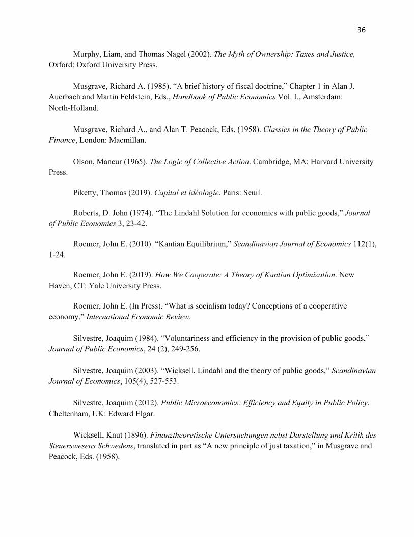
36

Murphy, Liam, and Thomas Nagel (2002). The Myth of Ownership: Taxes and Justice, Oxford: Oxford University Press.

Musgrave, Richard A. (1985). “A brief history of fiscal doctrine,” Chapter 1 in Alan J.

Auerbach and Martin Feldstein, Eds., Handbook of Public Economics Vol. I., Amsterdam: North-Holland.

Musgrave, Richard A., and Alan T. Peacock, Eds. (1958). Classics in the Theory of Public

Finance, London: Macmillan. Olson, Mancur (1965). The Logic of Collective Action. Cambridge, MA: Harvard University

Press.

Piketty, Thomas (2019). Capital et idéologie. Paris: Seuil.

Roberts, D. John (1974). “The Lindahl Solution for economies with public goods,” Journal of Public Economics 3, 23-42.

Roemer, John E. (2010). “Kantian Equilibrium,” Scandinavian Journal of Economics 112(1), 1-24.

Roemer, John E. (2019). How We Cooperate: A Theory of Kantian Optimization. New Haven, CT: Yale University Press.

Roemer, John E. (In Press). “What is socialism today? Conceptions of a cooperative economy,” International Economic Review.

Silvestre, Joaquim (1984). “Voluntariness and efficiency in the provision of public goods,”

Journal of Public Economics, 24 (2), 249-256. Silvestre, Joaquim (2003). “Wicksell, Lindahl and the theory of public goods,” Scandinavian

Journal of Economics, 105(4), 527-553. Silvestre, Joaquim (2012). Public Microeconomics: Efficiency and Equity in Public Policy.

Cheltenham, UK: Edward Elgar. Wicksell, Knut (1896). Finanztheoretische Untersuchungen nebst Darstellung und Kritik des

Steuerswesens Schwedens, translated in part as “A new principle of just taxation,” in Musgrave and Peacock, Eds. (1958).

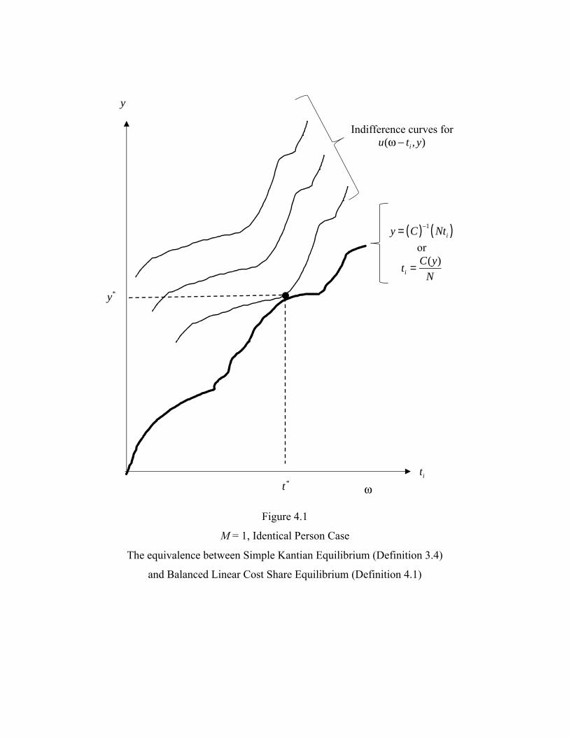
Figure 4.1

M = 1, Identical Person Case

The equivalence between Simple Kantian Equilibrium (Definition 3.4)

and Balanced Linear Cost Share Equilibrium (Definition 4.1)

y

y*

ω

Indifference curves for

u(ω − ti , y)

or

y = C( )−1 Nti( )

ti = C(y)N

t* ti

Figure 4.2

M = 1. The equivalence between Multiplicative Kantian Equilibrium (Definition 4.2)

and Balanced Linear Cost Share Equilibrium (Definition 4.1)

y

y*

ω i

Indifference curves for

ui (ω i − t j , y)

or

y = C( )−1 ti

ti* th

*h=1

N∑⎛⎝⎜

⎞⎠⎟

ti = ti*

th*

h=1

N∑C(y)

ti*

ti