INFORMATION AND INTERACTION

By

Dirk Bergemann, Tibor Heumann, and Stephen Morris

May 2017

COWLES FOUNDATION DISCUSSION PAPER NO. 2088

COWLES FOUNDATION FOR RESEARCH IN ECONOMICS YALE UNIVERSITY

Box 208281 New Haven, Connecticut 06520-8281

http://cowles.yale.edu/

Information and Interaction∗

Dirk Bergemann† Tibor Heumann‡ Stephen Morris§

May 22, 2015

Early and Preliminary Draft

Abstract

We study a linear interaction model with asymmetric information. We first characterize

the linear Bayes Nash equilibrium for a class of one dimensional signals. It is then shown that

this class of one dimensional signals provide a comprehensive description of the first and second

moments of the distribution of outcomes for any Bayes Nash equilibrium and any information

structure.

We use our results in a variety of applications: (i) we study the connections between

incomplete information and strategic interaction, (ii) we explain to what extent payoff envi-

ronment and information structure of a economy are distinguishable through the equilibrium

outcomes of the economy, and (iii) we analyze how equilibrium outcomes can be decomposed

to understand the sources of individual and aggregate volatility.

Jel Classification: C72, C73, D43, D83.

Keywords: Networks, Incomplete Information, Bayes Correlated Equilibrium, Volatility,

Moments Restrictions, Linear Best Responses, Quadratic Payoffs.

∗We acknowledge financial support through NSF Grant ICES 1215808.†Department of Economics, Yale University, New Haven, CT 06520, U.S.A., dirk.bergemann@yale.edu.‡Department of Economics, Yale University, New Haven, CT 06520, U.S.A., tibor.heumann@yale.edu.§Department of Economics, Princeton University, Princeton, NJ 08544, U.S.A. smorris@princeton.edu.

1

1 Introduction

1.1 Motivation

This paper studies an economy consisting of a finite number of agents with quadratic payoffs. The

best response of each agent is linear in the expectations of his payoff state (or payoff shock) and the

actions taken by other agents. The interaction matrix that describes the interaction between the

agents is allowed to be general and is not restricted to prescribe a uniform and symmetric interaction

among the agents. The payoff states of the agents are jointly normally distributed, but allowed to

be correlated according to an arbitrary variance-covariance matrix. The special cases of purely

idiosyncratic payoff states and purely common payoff states are allowed. The interaction structure

and the prior distribution of the agents payoff states together define the payoff environment of the

model. The information structure determines the information the agents have regarding their own

payoff state and the payoff states of other players. The information structure of the game allows

for private and incomplete information among the agents.

Heterogenous interactions and incomplete information are important elements in many economic

environments. For example, in macroeconomics a central question is to understand how heteroge-

neous input-output linkages and/or informational frictions contribute to aggregate volatility. Linear

interaction models have also been intensively used to understand social interactions. Here a central

question is how the network of interaction affects the efforts exerted by different players. Despite its

frequent use, there are only few contributions studying models with heterogenous interactions and

incomplete information. The focus of this paper is precisely to understand the interplay between the

payoff environment and the information structure in the determination of the equilibrium outcome.

We begin by studying a general class of one-dimensional signals. The signals that the agents

receive and the payoff shocks can be described by an arbitrary jointly normal distribution. We

characterize the set of linear Bayes Nash equilibrium of this game. The equilibrium strategies of

players in any linear Bayes Nash equilibria is characterized by two coefficients, one that determines

the strength with which an agent responds to his signal and one that determines a constant shift in

the agent’s action. The characterization of the equilibrium is surprisingly simple. The constant term

in an agent’s strategies depends only on the mean of agents payoff shocks and the interaction matrix

(but not on the information structure). Solving for the constant terms is isomorphic to solving the

Nash equilibrium under complete information. The strength with which an agent responds to his

signals depends on a modified interaction matrix and the correlation between an agent’s signal and

2

his payoff state. Given both of these elements, solving for the strength of the response is isomorphic

to solving for the equilibrium of a game under common values and complete information (where

the interaction matrix is equal to the aforementioned modified interaction matrix). The modified

interaction matrix is the Hadamard product (element wise product) of the interaction matrix and

the correlation matrix of the distributions of signals. That is, the interaction between agent i and

agent j is weighted by the correlation between the signals received by agent i and agent j. Hence,

the interaction between the uncertainty agents have on other agents actions and the interaction

network is completely captured by the modified interaction matrix.

Our characterization of equilibrium for one-dimensional signals is interesting for two reasons.

First, our characterization for one-dimensional signals allows us to formally connect problems of

heterogeneous interactions with problems of heterogenous information. In particular, the charac-

terization of linear Bayes Nash equilibrium relies only on a modified interaction matrix in which

strategic interactions and incomplete information (through the correlations in agents signals) enter

symmetrically. As an application, we develop a “informationally rich” Beauty Contest. That is, we

consider a standard Beauty Contest (as introduced by Morris and Shin (2002)), but we consider

a finite number of agents with heterogenous information. We show that the techniques developed

for complete information equilibria and common values (see Ballester, Calvo-Armengol, and Zenou

(2006)) extend directly to this model. Yet, instead of applying the methods to the matrix of strategic

interaction, we apply the methods to the variance-covariance matrix of errors in agents’ signals.

Second, it allow us to understand how the payoff environment and information structure shape

the equilibrium outcome of the game. In particular, it illustrates how different payoff environments

and information structures can lead to the same distribution of actions in equilibrium. Specifically

we answer the following question. Consider an economy consisting of N agents that interact through

some interaction network, have payoff shocks heterogeneously distributed and have incomplete

information on the realization of the payoff shocks. Say an analyst can observe the joint distribution

of actions taken by the players, but does not observe the details on the interaction network, agents’

payoff shocks or the information structure of agents. The analyst is interested in studying what

combinations of these three elements of an economy could give rise to the observed distribution of

actions. We show that any joint distribution of outcomes can be rationalized by any of the following

three models:

1. Agents have complete information, no strategic interactions but heterogenous payoff shocks;

2. Agents have complete information, independent payoff shocks but heterogenous strategic in-

3

teractions;

3. Agents have no strategic interactions, independent payoff shocks but incomplete information.

Hence, we can see that heterogenous interactions, heterogenous payoff shocks and incomplete

information – considered independently – yield the same predictions over the joint distribution

of actions in equilibrium. It is therefore interesting to ask how do these mechanisms differ. In

particular, we study what are the feasible outcomes for a fixed payoff environment.

We then proceed to characterize all outcomes that can be rationalized as a Bayes Nash equilib-

rium for some information structure. That is, we fix a payoff environment and look for all possible

joint distributions of payoff shocks and actions (henceforth, an outcome) that can be rationalized

as a Bayes Nash equilibrium, for some information structure. To characterize the set of joint dis-

tributions that are rationalizable as an outcome for some payoff environment, we define a Bayes

correlated equilibrium (see Bergemann and Morris (2015)). A Bayes correlated equilibrium con-

sists of a joint distribution of outcomes that satisfies an obedience condition. Notably, there is

no reference to an information structure in the definition of a Bayes correlated equilibrium, but

just an obedience constraint defined over the outcome variables themselves. A direct extension of

an epistemic result found in Bergemann and Morris (2015) shows that the set of Bayes correlated

equilibrium characterizes all outcomes that are rationalizable as a Bayes Nash equilibrium for some

information structure. As we focus attention on Bayes correlated equilibrium that are normally

distributed, these are completely characterized by the first and second moments of the distribution.

We show that the first moment of the economy is determined by the interaction matrix and the

first moments of the payoffs state, and hence completely determined by the payoff environment.

This is reminiscent of the characterization of the constant term in a linear Bayes Nash equilibrium

for one-dimensional signals. Consequently, we focus our analysis on the second moments of the

distribution, namely variance of outcome variables and the correlation between outcome variables.

The characterization of the second moments has two parts. The only constraint on the correla-

tion matrix is the purely statistical property that it must be positive semi-definite. On the other

hand, the variance of an agent’s action is determined by the correlations of agents actions and the

interaction matrix. This is reminiscent of the characterization of the linear term in a linear Bayes

Nash equilibrium for one-dimensional signals. The only difference is that, instead of adjusting the

interaction matrix by the correlation in the signals of the agents, the interaction matrix is adjusted

by the correlation of the actions of the agents. The conditions on the first two moments, the indi-

vidual variance and the correlations completely characterize the set of distributions that are Bayes

4

correlated equilibria.

We establish that the only robust implication of the interaction structure on outcomes is through

the variance of agents’ actions. The impact of the interaction matrix is weighted by the correla-

tion between agents’ actions. Nevertheless, the interaction matrix imposes no restrictions on the

set of feasible correlations. On the other hand, the correlation matrix of payoff states imposes

some restrictions on the set of feasible correlations of outcome (namely, actions and payoff states)

through the condition that this matrix must be positive semi-definite. Although a fixed correlation

matrix of payoff states imposes no restrictions on the set of feasible correlation matrix of actions,

a fixed correlation matrix of payoff states jointly with a fixed correlation matrix of actions imposes

restrictions on the set of feasible correlations between actions and payoff states.

An important aspect of the Bayes correlated equilibrium is that all conditions derived remain

necessary for any outcome of any Bayes Nash equilibrium even if the normality assumption is

relaxed. This implies that these conditions are also necessary for non-linear equilibria. The descrip-

tion of a Bayes correlated equilibrium shows that the class of one-dimensional signals previously

studied provide a maximal description of all first and second moments achievable by any Bayes Nash

equilibrium. That is, any combination of first and second moment of outcomes that can be achieved

by a Bayes Nash equilibrium for some information structure, can also be obtained by a Bayes Nash

equilibrium in which agents receive one-dimensional signals as the ones previously studied. This

also holds across non-normal and non-linear equilibria.

A Bayes correlated equilibrium provide us with a compact description of outcomes, without the

need to make explicit reference to a specific information structure. This allow us to analyze the set

of outcomes without the need to define a information structure and derive the associated equilibrium

strategy profile. We first show that actions can be decomposed in terms of fundamentals and noise.

Thus, the actions of the players can always be written as a linear combination of payoff shocks and

noise terms. Hence, the equilibrium outcome of a game provides sufficient information to establish

how much of the volatility in actions is driven by fundamentals and how much is driven by noise.

A particular class of Bayes correlated equilibrium consists of outcomes in which the actions are

completely measurable with respect to the fundamentals. That is, there is no noise in players’

actions, and hence we call them noise free. A Bayes Nash equilibrium under complete information

always induces a noise free outcome. But importantly, there is a continuum of other noise free

outcomes which do not correspond to the outcome of the Bayes Nash equilibrium under complete

information.

5

Finally, we show how the aggregate volatility of the actions can be decomposed into two terms:

the individual volatility of each action and the correlations between the actions. The correlations

between the actions determines the aggregation of the individual volatility in individual actions.

The individual volatility of each agent’s action can also be decomposed into two terms: the response

of each agent to the fundamental payoff shock and the response to the other agents’ actions.

1.2 Related Literature

Methodologically our paper is related to the literature that derives the predictions of a game for all

information structure at once, in particular via the use of the Bayes correlated equilibrium for game

of incomplete information. In Bergemann and Morris (2015), two of us considered this problem

in an abstract game theoretic setting. There we showed that a general version of Bayes correlated

equilibrium characterizes the set of outcomes that could arise in any Bayes Nash equilibrium of an

incomplete information game where agents may or may not have access to more information beyond

the given common prior over the fundamentals. In Bergemann and Morris (2013) we pursued this

argument in detail and characterized the set of Bayes correlated equilibria in the class of games with

quadratic payoffs and normally distributed uncertainty, but restricted our attention to the special

environment with purely aggregate shocks, or pure common values. In Bergemann, Heumann, and

Morris (2015) we generalized the environment to a symmetric model with interdependent values, a

continuum of agents and symmetric interactions.

Many of the connections we pursue in this paper between strategic interaction and incomplete

information are not new. The equilibrium behavior in arbitrary networks and in arbitrary infor-

mation structures are tightly linked as argued by Morris (1997). The stylized model proposed here

allows us to get sharper connections between both problems. Moreover, we study systematically

how different models can yield identical outcomes, making the connection transparent.

Our paper is related to a large literature that studies how heterogenous interactions affect the

outcome of the game. An important question is macroeconomics is to understand how the shocks

to individual firms translate into aggregate volatility. To answer this question several mechanisms

have been proposed. Gabaix (2011) considered a complete information economy in which firm-level

idiosyncratic shocks translate into aggregate fluctuations when the firm size distribution is suffi-

ciently heavy-tailed and the largest firms contribute disproportionately to the aggregate output.

In Acemoglu, Carvalho, Ozdaglar, and Tahbaz-Salehi (2012) firms interact through input-output

linkages under complete information, and it is the heterogenous interactions between firms that

6

cause aggregate volatility to not vanish. In particular, the shocks of some firms have dispropor-

tionate high impact on aggregate volatility due to the interaction matrix. Finally, in Angeletos

and La’O (2013) informational frictions cause firms to respond to a common noise term, which

causes aggregate volatility not to vanish. We provide a model that allows us to study these three

transmission mechanisms within a unified framework. Moreover, we can show to what extent these

mechanisms can be separated by the observable outcomes, and to what extent different mechanisms

are indistinguishable from the outcome of the game.

In contrast to much of the literature on networks, with the notable exception of de Marti and

Zenou (2013), we are interested in analyzing the behavior of the agents under incomplete and

asymmetric information, and thus we need to specify an information structure, a type space for the

agents. Similar to us, de Marti and Zenou (2013) consider a linear quadratic model but restrict

attention to a model with pure common values, i.e. the payoff state of all the agents is assumed to

be the same, and they consider information structures with either binary or finitely many signals.

Importantly, our papers differ methodologically as well. While de Marti and Zenou (2013) focus on

understanding equilibria using the Katz-Bonacich centralities, we characterize equilibria in terms

of the second moments of the joint distribution of payoff states and actions. We also show that the

one-dimensional information structures provide a comprehensive description of all first and second

moments that can be a achieved by any Bayes Nash equilibrium of any information structure.

Imperfect information, information gathering and communication are themes that also appear in

Calvo-Armengol and de Marti (2009) and Calvo-Armengol, de Marti, and Prat (2015).

In a recent contribution, Blume, Brock, Durlauf, and Jayaraman (2015) provide a comprehensive

analysis of identification in linear interaction models. They allow for agents to get public information

and private information. The private information of the agents is always independent across agents

and informative on each agent’s own payoff shock. This implies that the second-order beliefs and

all higher-order beliefs are all common knowledge. By contrast, we provide restrictions on the

set of outcomes that hold across all possible information structures. Although, we do not offer a

systematic analysis of identification, we hope our work complements the study of identification in

linear frameworks.

The rest of the paper proceeds as follows. In Section 2 we provide the model. In Section 3 we

study the Bayes Nash equilibria of the model under normally distributed information structures.

In Section 4 we define and characterize the Bayes correlated equilibria of the economy.

7

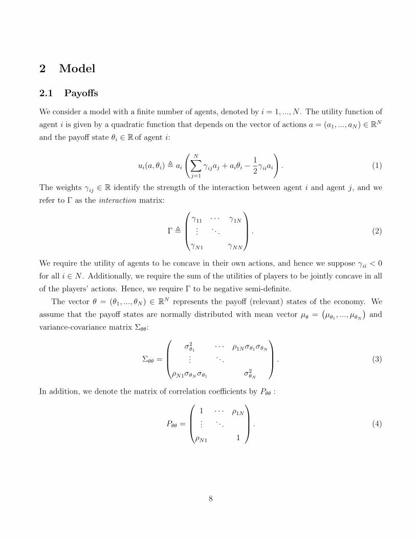
2 Model

2.1 Payoffs

We consider a model with a finite number of agents, denoted by i = 1, ..., N . The utility function of

agent i is given by a quadratic function that depends on the vector of actions a = (a1, ..., aN) ∈ RN

and the payoff state θi ∈ R of agent i:

ui(a, θi) , ai

(N∑j=1

γijaj + aiθi −1

2γiiai

). (1)

The weights γij ∈ R identify the strength of the interaction between agent i and agent j, and we

refer to Γ as the interaction matrix:

Γ ,

γ11 · · · γ1N...

. . .

γN1 γNN

. (2)

We require the utility of agents to be concave in their own actions, and hence we suppose γii < 0

for all i ∈ N . Additionally, we require the sum of the utilities of players to be jointly concave in all

of the players’ actions. Hence, we require Γ to be negative semi-definite.

The vector θ = (θ1, ..., θN) ∈ RN represents the payoff (relevant) states of the economy. We

assume that the payoff states are normally distributed with mean vector µθ =(µθ1 , ..., µθN

)and

variance-covariance matrix Σθθ:

Σθθ =

σ2θ1

· · · ρ1Nσθ1σθN...

. . .

ρN1σθNσθ1 σ2θN

. (3)

In addition, we denote the matrix of correlation coefficients by Pθθ :

Pθθ =

1 · · · ρ1N...

. . .

ρN1 1

. (4)

8

2.2 Information Structure

We are concerned with environments in which each agent has less than complete information about

the vector of payoff states, and thus we consider environments with incomplete information.

Each agent is assumed to receive a vector of noisy signals si , (si1, ..., siK) ∈ RK about the

payoff state vector (θ1, ..., θN), for some finite K. The vector si of signals that agent i receives yields

the information set of agent i, which we sometimes denote alternatively by Ii , (si1, ..., siK). We

assume that the signals of all the agents are jointly normally distributed with the payoff state, and

thus given by a joint distribution of states and signals:

θ1

...

θN

s1

...

sN

∼ N

µθ1...

µθNµs1...

µsN

,

(Σθθ Σθs

Σsθ Σss

). (5)

We provide some simple examples of possible information structures.

Example 1: Complete Information. We can easily accommodate the case of complete infor-

mation. This can be explicitly written by assuming K = N , and assuming agents get signals that

are described as follows:

∀i, j ∈ N, sij = θj.

Example 2: Noisy Signal on Own Payoff State. A standard information structure is to

assume agents observe a noisy signal on their own payoff shock. This can be explicitly written by

assuming K = 1, and assuming agents get signals that are described as follows:

∀i ∈ N, si = θi + εi,

where now (ε1, ..., εN) are jointly independent of (θ1, ..., θN) and have some variance-covariance

matrix Σεε.

Example 3: Noise Free Signals. A less standard information structure is to assume that the

agents have incomplete information, but that their signals are measurable with respect to (θ1, ..., θN).

For the case of K = 1, we can assign a vector of weights λi , (λi1, ..., λiN), such that the signal

agent i receives can be written as follows:

∀i ∈ N, si ,∑j∈N

λijθj.

9

Once again, we would like to emphasize that under this information structure, agents are uncertain

about the realization of their own shock. Yet, there is no noise in agents signals.

3 Bayes Nash Equilibrium

3.1 Solution Concept

We consider the game with incomplete information. The (possibly mixed) strategy of each agent is

a mapping from the private signal si ∈ RK to the action ai ∈ R:

ai : RK → ∆ (R) .

Given the quadratic payoff structure, the best response of each agent i is given by the linear

condition:

ai = − 1

γiiE[θi +

∑j 6=i

γijaj|si]. (6)

We define the Bayes Nash equilibrium of this game.

Definition 1 (Bayes Nash Equilibrium)

A Bayes Nash Equilibrium is defined by functions a∗i : RK → R such that:

∀i ∈ N,∀si ∈ RK , E[θi +∑j∈N

γija∗j(sj)|si] = 0. (7)

It is worth mentioning that in any Bayes Nash equilibrium, the expected utility of agent i ∈ Nis proportional to the individual volatility of his action.

Lemma 1 (Equilibrium Welfare)

Let a∗i : RK → R be a Bayes Nash equilibrium, then:

E[a∗i (si)(θi +∑j∈N

γija∗j(sj)−

γii2a∗i (si))] = −γii

2σ2a −

γii2µ2a.

Lemma 1 will be useful to interpret our results. In particular, we often study the actions of

the players in terms of their first and second moments. It is then useful to keep in mind that the

first and second moments of the actions allow us to calculate the expected utility of the agents. In

particular, a higher individual volatility implies a higher expected utility.

10

3.2 Complete Information

As a benchmark, it is useful to describe the Nash equilibrium under complete information. The

equilibrium action profile a∗ is the result of the best response of each player given by

0 = θi +∑j∈N

γija∗j ,

and in vector matrix format we obtain the unique Nash equilibrium (a∗1, ..., a∗N):

a∗1...

a∗N

= −Γ−1

θ1

...

θN

. (8)

The analysis of this game under complete information is standard in the literature. In particular,

Ballester, Calvo-Armengol, and Zenou (2006) study this model and relate the actions taken by each

player to his Bonacich centrality on the network. We briefly review some of the relevant results for

the complete information case here. Let G be some arbitrary matrix and φ be some number, we

define the vector b(G, φ) to be the Bonacich centrality measure of G using parameter φ as follows:

b(G, φ) , (I− φG)−1 ·

1...

1

.

For an arbitrary interaction matrix Γ, we can describe each agent’s best response in terms of the

Bonacich centrality measure of Γ.

We now illustrate briefly how different papers have used this measure of centrality. Consider

the case in which agents have complete information and common values (when we discuss models of

common values, we denote the common shock to all agents by θ). The best responses of the agents

11

are given by:1 a1

...

aN

= θ · b(Γ + I, 1). (9)

Hence, the response of each agent is proportional to his measure of Bonacich centrality, this model

is studied in detail in Ballester, Calvo-Armengol, and Zenou (2006).

Consider next the general case in which the payoff states are not common, but we focus on the

average action taken by players. In the complete information equilibrium the average action taken

by the players is given by:

a ,1

N

∑i∈N

ai =

θ1

...

θN

· b(Γ′ + I, 1). (10)

Hence, the importance of payoff shock θi for the average action is proportional to the Bonacich

centrality measure of the matrix Γ′ + I. A detailed analysis of how the structure of the network

affects aggregate volatility is pursued in Acemoglu, Carvalho, Ozdaglar, and Tahbaz-Salehi (2012).

Finally, we observe that the complete information equilibrium induces a joint distribution of

variables (θ1, ..., θN , a1, ..., aN) that is jointly normally distributed. Moreover, using standard results

for normal distributions, we have that the first and second moments of the joint distribution of

variables are given by:

µa = Γ · µθ, (11)

and (Σθθ Σθa

Σaθ Σaa

)=

(Σθθ Γ−1Σθθ

Σθθ (Γ−1)T

Γ−1Σθθ (Γ−1)T

). (12)

Since normal distributions are uniquely determined by their first and second moments, (11) and

(12) uniquely determine the distribution of (θ1, ..., θN , a1, ..., aN).

1The fact that the Bonacich centrality vector is calculated over Γ + I instead of Γ should be considered as a

normalization. If γii = −1 for all i ∈ N , then the diagonal of Γ + I is equal to 0. Hence, Γ + I corresponds to the

part of Γ that corresponds to the interactions between agents. Usually the interaction matrix is considered to be a

matrix equal to Γ outside the diagonal and equal to 0 on the diagonal, hence separating the part that corresponds

to interactions between agents with the part that corresponds to the concavity of the payoff function of agents. In

such case there is no normalization of adding the identity matrix to the Bonacich centrality vector. The notation we

use throughout the paper provides a more compact characterizations for all of our results.

12

3.3 One-Dimensional Signals

We now characterize the Bayes Nash equilibrium of the game when agents receive arbitrary one-

dimensional signals (that is, si = si1). Without loss of generality we normalize the signals to have

0 mean and a variance of 1 (that is, var(si) = 1 and E[si] = 0). Therefore, the variance-covariance

matrix simply equals the correlation matrix, or Σss = Pss. We look for Bayes Nash equilibria in

linear strategies, and thus we need to identify parameters (α1, ..., αN) and (β1, ..., βN) such that:

∀i, a∗i (si) = αisi + βi.

Written in terms of the first order conditions (6), we need to solve:

∀i ∈ N, E[∑j∈N

γij(αjsj + βj) + θi|si] = 0.

Proposition 1 (Characterization for One Dimensional Signals: Strategy)

The linear strategies (α∗1, ..., α∗N) and (β∗1, ..., β

∗N) form a Bayes Nash equilibrium if and only if:

β∗1...

β∗N

= −Γ−1 ·

µθ1

...

µθN

(13)

and α∗1...

α∗N

= −(Pss ◦ Γ)−1 ·

cov(θ1, s1)

...

cov(θN , sN)

. (14)

The product between the correlation matrix and the interaction matrix (Pss◦Γ) is the Hadamard

product of the two matrices, that is the element-wise multiplication ρij ·γij. Proposition 1 establishes

a strong connection between the informational frictions and the network effects. The constant

component in agents action βi is the product of the interaction matrix and the mean of all the

agents payoff states. The response of agents to their signal is the product of an adjusted interaction

matrix (Pss◦Γ)−1. The interaction matrix is adjusted by the information agents have on the actions

taken by other agents (given by the correlation between agents signals).

Given the equilibrium, we can describe the joint distribution of actions and payoff states

(θ1, ..., θN , a1, ..., aN). Once again, as we keep the normality of the joint distribution of outcomes,

the first and second moment will suffice to characterize this distribution.

13

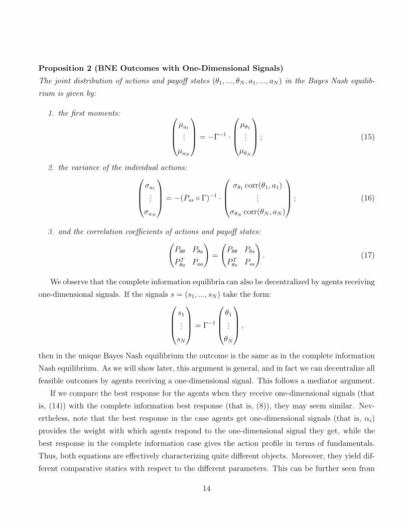
Proposition 2 (BNE Outcomes with One-Dimensional Signals)

The joint distribution of actions and payoff states (θ1, ..., θN , a1, ..., aN) in the Bayes Nash equilib-

rium is given by:

1. the first moments: µa1

...

µaN

= −Γ−1 ·

µθ1

...

µθN

; (15)

2. the variance of the individual actions:σa1

...

σaN

= −(Pss ◦ Γ)−1 ·

σθ1 corr(θ1, a1)

...

σθN corr(θN , aN)

; (16)

3. and the correlation coefficients of actions and payoff states:(Pθθ Pθa

P Tθa Paa

)=

(Pθθ Pθs

P Tθs Pss

). (17)

We observe that the complete information equilibria can also be decentralized by agents receiving

one-dimensional signals. If the signals s = (s1, ..., sN) take the form:s1

...

sN

= Γ−1

θ1

...

θN

,

then in the unique Bayes Nash equilibrium the outcome is the same as in the complete information

Nash equilibrium. As we will show later, this argument is general, and in fact we can decentralize all

feasible outcomes by agents receiving a one-dimensional signal. This follows a mediator argument.

If we compare the best response for the agents when they receive one-dimensional signals (that

is, (14)) with the complete information best response (that is, (8)), they may seem similar. Nev-

ertheless, note that the best response in the case agents get one-dimensional signals (that is, αi)

provides the weight with which agents respond to the one-dimensional signal they get, while the

best response in the complete information case gives the action profile in terms of fundamentals.

Thus, both equations are effectively characterizing quite different objects. Moreover, they yield dif-

ferent comparative statics with respect to the different parameters. This can be further seen from

14

the characterization of the variance covariance matrix in the complete information, given by (12),

which seems qualitatively very different from the characterization of the incomplete information

given by (16). Even though both characterizations are very different in general, there is a connec-

tion between the characterization of an equilibrium when agents get one-dimensional signals, and

the complete information equilibria in a common value environment. We explain this connection in

Section 3.6.

3.4 Three Rationalizations

So far we have studied Bayes Nash equilibrium under one-dimensional signals and under complete

information. We now study how different payoff environments and information structures can

decentralize different outcomes. To be more concise, we consider the following question. Fix a

variance-covariance matrix of actions Σaa.2 Now consider the question of what combination of

payoff environment and information structures would decentralize Σaa as the outcome of a Bayes

Nash equilibrium. We answer this questions in the following Proposition. Before we provide the

proposition, we should note that the proposition relies on taking square roots of a matrix. Although

this is done the natural way, we are more specific on this in Lemma 2.

Proposition 3 (Three Rationalizations Results)

The variance-covariance matrix of actions Σaa is the outcome of a Bayes Nash equilibrium in the

following environments:

1. agents do not interact (Γ = I), agents have complete information and the distribution over

payoff states is given by:

Σθθ = Σaa; (18)

2. agents have complete information, payoff states are independently distributed with a variance

of 1 (Σθθ = I), and the interaction matrix is given by any solution to:

Γ = Σ−1/2aa , (19)

such that Γ is negative semi-definite (and such a solution always exists);

2The only restriction on Σaa to be a valid varinace/covariance of actions is that it must be positive semi-definite

15

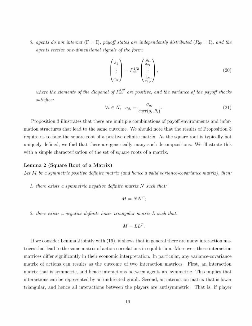
3. agents do not interact (Γ = I), payoff states are independently distributed (Pθθ = I), and the

agents receive one-dimensional signals of the form:s1

...

sN

= P 1/2aa

θ1σθ1...θNσθN

, (20)

where the elements of the diagonal of P1/2aa are positive, and the variance of the payoff shocks

satisfies:

∀i ∈ N, σθi =σai

corr(si, θi). (21)

Proposition 3 illustrates that there are multiple combinations of payoff environments and infor-

mation structures that lead to the same outcome. We should note that the results of Proposition 3

require us to take the square root of a positive definite matrix. As the square root is typically not

uniquely defined, we find that there are generically many such decompositions. We illustrate this

with a simple characterization of the set of square roots of a matrix.

Lemma 2 (Square Root of a Matrix)

Let M be a symmetric positive definite matrix (and hence a valid variance-covariance matrix), then:

1. there exists a symmetric negative definite matrix N such that:

M = NNT ;

2. there exists a negative definite lower triangular matrix L such that:

M = LLT .

If we consider Lemma 2 jointly with (19), it shows that in general there are many interaction ma-

trices that lead to the same matrix of action correlations in equilibrium. Moreover, these interaction

matrices differ significantly in their economic interpretation. In particular, any variance-covariance

matrix of actions can results as the outcome of two interaction matrices. First, an interaction

matrix that is symmetric, and hence interactions between agents are symmetric. This implies that

interactions can be represented by an undirected graph. Second, an interaction matrix that is lower

triangular, and hence all interactions between the players are antisymmetric. That is, if player

16

i responds to the action of player j, then player j does not interact with player i. Moreover, in

the latter case interactions are nested (as suggested by the lower triangular form of the interaction

matrix).

We now illustrate this by means of a simple example. We consider the case of N = 3 with the

following variance-covariance matrix of actions:

Σaa , var

a1

a2

a3

=

132

52√

25

2√

25

2√

2154

114

52√

2114

154

. (22)

Corollary 1 (Three Rationalizations Results: Numerical Example)

Let Σaa be defined by (22), then Σaa is the outcome of a Bayes Nash equilibrium in the following

environments:

1. agents do not interact (Γ = I), agents have complete information and the distribution over

payoff states is given by:

Σθθ = Σaa =

132

52√

25

2√

25

2√

2154

114

52√

2114

154

; (23)

2.a. agents have complete information, payoff states are independently distributed (Pθθ = I) with

a variance of 1 and the interaction matrix is given by:

Γ =

− 5

121

12√

21

12√

21

12√

2−17

24724

112√

2724

−1724

; (24)

2.b. agents have complete information, payoff states are independently distributed (Σθθ = I) with

a variance of 1 and the interaction matrix is given by:

Γ =

−√

132

65

12√

135

12√

13

0 −√

1526

11√390

0 0 − 2√15

; (25)

17

3.a. agents do not interact (Γ = I), payoff states are independently distributed (Σθθ = I), agents

receive one-dimensional signals of the form:s1

s2

s3

=

1√

539

√539

0√

3439

59√

2663

5

0 08√

317

5

θ1σθ1θ2σθ2θ3σθ3

(26)

and the variance of payoff shocks is given by:σθ1

σθ2

σθ3

=

496

5353√

3442

85

6√

317

;

3.b. agents do not interact (Γ = I), payoff states are independently distributed (Pθθ = I), agents

receive one-dimensional signals of the form:s1

s2

s3

=

0.97... 0.15... 0.15...

0.15... 0.90... 0.39...

0.15... 0.39... 0.90...

θ1σθ1θ2σθ2θ3σθ3

and the variance of payoff shocks is given by:

σθ1

σθ2

σθ3

=

6.66...

4.13...

4.13...

.

We can see that any variance-covariance matrix of actions can be decentralized either by the

appropriate payoff shocks, the appropriate interaction matrix (and assuming complete information)

or under the appropriate informational frictions. Moreover, we can see that very different interaction

matrices can lead to the same outcomes.

3.5 Interaction between Strategic and Informational Effects

We now illustrates by means of a simple example how the information structure interacts with the

interaction matrix. We consider the case of common values (that is, θi = θj = θ for all i, j ∈ N). We

18

consider the following two networks. First, we consider the case in which agents interact through a

uniform interaction network. In particular, we assume the following parametrization:

∀i, j ∈ N, γuii = −1 +r

Nand γuij =

r

N.

For N = 4, this can be written as follows:

Γu ,

−1 0 0 0

0 −1 0 0

0 0 −1 0

0 0 0 −1

+r

N

1 1 1 1

1 1 1 1

1 1 1 1

1 1 1 1

.

Second, we consider a star network. We consider agent 1 to be the center of the network. We will

consider a parametrization that allow us to change the relative strength of the interactions between

periphery and center. We provide the parametrization and the choice of parametrization should

become transparent following Proposition 3:

∀i, j ∈ N with i, j 6= 1, γsii , 1 ; γs11 , −1 +r

N; γsij = 0 ; γs1i =

r

Nand γsi1 = r,

with:

c1 =Nc2(r − 1)− r +N

(N − 1)c2r.

For N = 4, this can be written as follows:

Γs ,

−1 0 0 0

0 −1 0 0

0 0 −1 0

0 0 0 −1

+

rN

c1rN

c1rN

c1rN

c2r 0 0 0

c2r 0 0 0

c2r 0 0 0

.

We consider values of r ≥ 0. This is to keep the discussion focused on the case of strategic

complementarities, and hence not having to worry about comparative statics that change sign

when we move from strategic complementarities to strategic substitutabilities. It is clear that

the calculations and main intuitions do not hinge on this. It is also clear that c2, c1 cannot take

arbitrary values, as the strategic interaction matrix must be negative definite. Nevertheless, we

will not worry about this, and we will just work for values of c2, c1 near 1. As we know that for

c1 = c2 = 1 the interaction matrix is negative definite, then our results apply for values c1 = c2 ≈ 1.

Our parametrization allow us to provide a simple characterization for the complete information

equilibrium.

19

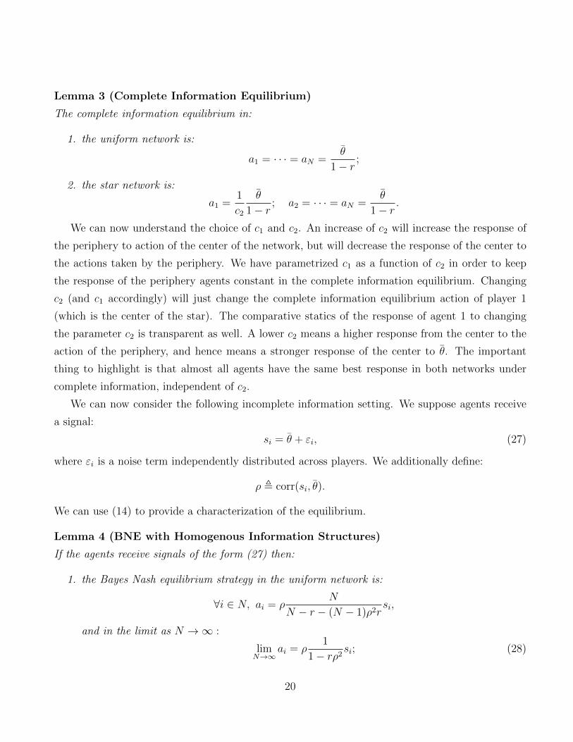
Lemma 3 (Complete Information Equilibrium)

The complete information equilibrium in:

1. the uniform network is:

a1 = · · · = aN =θ

1− r;

2. the star network is:

a1 =1

c2

θ

1− r; a2 = · · · = aN =

θ

1− r.

We can now understand the choice of c1 and c2. An increase of c2 will increase the response of

the periphery to action of the center of the network, but will decrease the response of the center to

the actions taken by the periphery. We have parametrized c1 as a function of c2 in order to keep

the response of the periphery agents constant in the complete information equilibrium. Changing

c2 (and c1 accordingly) will just change the complete information equilibrium action of player 1

(which is the center of the star). The comparative statics of the response of agent 1 to changing

the parameter c2 is transparent as well. A lower c2 means a higher response from the center to the

action of the periphery, and hence means a stronger response of the center to θ. The important

thing to highlight is that almost all agents have the same best response in both networks under

complete information, independent of c2.

We can now consider the following incomplete information setting. We suppose agents receive

a signal:

si = θ + εi, (27)

where εi is a noise term independently distributed across players. We additionally define:

ρ , corr(si, θ).

We can use (14) to provide a characterization of the equilibrium.

Lemma 4 (BNE with Homogenous Information Structures)

If the agents receive signals of the form (27) then:

1. the Bayes Nash equilibrium strategy in the uniform network is:

∀i ∈ N, ai = ρN

N − r − (N − 1)ρ2rsi,

and in the limit as N →∞ :

limN→∞

ai = ρ1

1− rρ2si; (28)

20

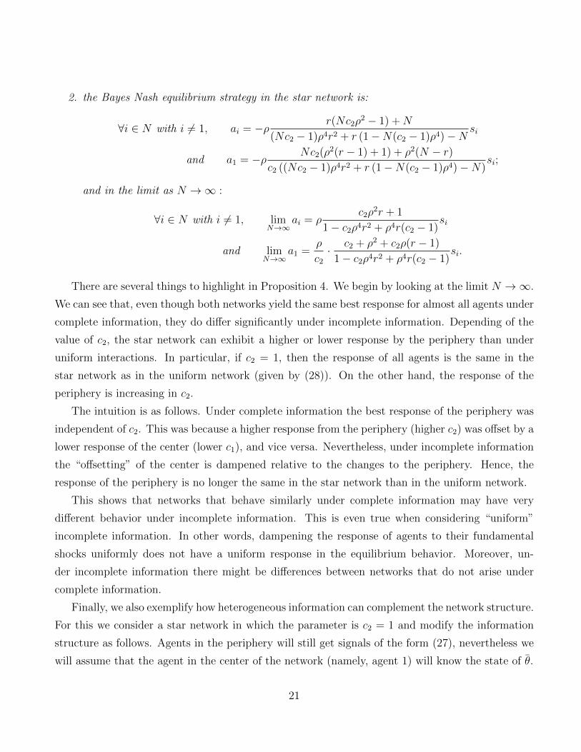
2. the Bayes Nash equilibrium strategy in the star network is:

∀i ∈ N with i 6= 1, ai = −ρ r(Nc2ρ2 − 1) +N

(Nc2 − 1)ρ4r2 + r (1−N(c2 − 1)ρ4)−Nsi

and a1 = −ρ Nc2(ρ2(r − 1) + 1) + ρ2(N − r)c2 ((Nc2 − 1)ρ4r2 + r (1−N(c2 − 1)ρ4)−N)

si;

and in the limit as N →∞ :

∀i ∈ N with i 6= 1, limN→∞

ai = ρc2ρ

2r + 1

1− c2ρ4r2 + ρ4r(c2 − 1)si

and limN→∞

a1 =ρ

c2

· c2 + ρ2 + c2ρ(r − 1)

1− c2ρ4r2 + ρ4r(c2 − 1)si.

There are several things to highlight in Proposition 4. We begin by looking at the limit N →∞.

We can see that, even though both networks yield the same best response for almost all agents under

complete information, they do differ significantly under incomplete information. Depending of the

value of c2, the star network can exhibit a higher or lower response by the periphery than under

uniform interactions. In particular, if c2 = 1, then the response of all agents is the same in the

star network as in the uniform network (given by (28)). On the other hand, the response of the

periphery is increasing in c2.

The intuition is as follows. Under complete information the best response of the periphery was

independent of c2. This was because a higher response from the periphery (higher c2) was offset by a

lower response of the center (lower c1), and vice versa. Nevertheless, under incomplete information

the “offsetting” of the center is dampened relative to the changes to the periphery. Hence, the

response of the periphery is no longer the same in the star network than in the uniform network.

This shows that networks that behave similarly under complete information may have very

different behavior under incomplete information. This is even true when considering “uniform”

incomplete information. In other words, dampening the response of agents to their fundamental

shocks uniformly does not have a uniform response in the equilibrium behavior. Moreover, un-

der incomplete information there might be differences between networks that do not arise under

complete information.

Finally, we also exemplify how heterogeneous information can complement the network structure.

For this we consider a star network in which the parameter is c2 = 1 and modify the information

structure as follows. Agents in the periphery will still get signals of the form (27), nevertheless we

will assume that the agent in the center of the network (namely, agent 1) will know the state of θ.

21

Lemma 5 (Equilibria for heterogenous information structure)

In the Bayes Nash equilibrium of the star network and an information structure in which player 1

knows the realization of θ, the best response of agents is given by:

∀i ∈ N with i 6= 1, ai = ρ(Nρ− 1)r +N

N − (N − 1)ρ2r2 − rsi,

and a1 =(N − 1)ρr +N

N − (N − 1)ρ2r2 − rθ.

In the limit as N →∞:

∀i ∈ N with i 6= 1, limN→∞

ai = ρ1

1− ρrsi

and limN→∞

a1 =1

1− ρr.

The interesting aspect of Proposition 5 is the response of the periphery agents to their signals

when N → ∞. We remind the reader that, for c2 = 1, the response of the periphery agents when

the central agent received a noisy signal in the limit as N → ∞ was the same as the uniform

interaction (and equal to (28)). Hence, when the central agent receives a more precise signal, all

periphery agents respond stronger to their own signal as well. It is clear that if interactions are

homogenous, then changing the information of an individual would not change the equilibrium in

the limit as N →∞. This shows that improving the information structure of particular individuals

in the network can have large effects in the equilibrium. We analyze the problem of evaluating the

centrality of an agent with respect to the information structure in the following section.

3.6 Information Centrality

We now provide the connection between the complete information equilibria with common values

and the incomplete information equilibria in which agents get generic one-dimensional signals. We

assume that each agent gets a signal si, where as usual (θ1, ..., θN , , s1, ..., sN) are jointly normally

distributed. Further more, we assume that no agent has better information about their own payoff

state than any other agent:3

∀i, j ∈ N, corr(si, θi) = corr(sj, θj) , ρ. (29)

3It is clear that this assumption can be easily relaxed. Yet, this allow us to normalize the part of the response of

agents to their signals that comes directly from their payoff shock, and not from their interactions with others.

22

Note that we have made no assumptions on the correlations between signals beyond (29). In

particular, we are accommodating that agents get a common public signal or the possibility that

they get conditionally independent private signals.

To get the best response of agents we can use Proposition 2. In particular, we can write (16) as

follows:

α = − cov(s, θ) · (Σss ◦ Γ)−1 ·

1...

1

, (30)

From (30)-(31) we can see that the response of an agent to the generic one-dimensional signal

is isomorphic to an agent’s response to a shock in a common value environment. In particular,

rewriting (8) for the case in which agents have common values, we get:

ai = −θ ·

Γ−1 ·

1...

1

. (31)

By using the modified interaction matrix

Γ , (Σss ◦ Γ), (32)

instead of just Γ and a modified payoff state θ = cov(s, θ) we can see that the problem of find-

ing the best response of agents in the incomplete information environment is isomorphic to the

problem of solving complete information games with common values. We should highlight that

the heterogeneity does not necessarily come from the interactions, but it can also come from the

information. Moreover, in the best response they are indistinguishable, as they enter symmetrically

in the modified interaction matrix (32).

We now consider a “informationally rich” Beauty Contest. We consider N agents that have

common values and just an aggregate interaction which is equal for all agents. The best response

of agents is given by:

ai = E[θ +r

N

∑i∈N

ai].

In the notation of the paper, we have that γij = r/N and γii = −1 + r/N . Then, we can write Γ

as follows:

Γ , γ ◦ Σss = (rΣss − I).

23

where I is the identity matrix. We assume agents get signals of the form:

si = ρθi +√

1− ρ2εi, (33)

where εi is an error term with variance 1 and some arbitrary correlation matrix Pεε across players.

The variance covariance matrix of signals Σss can be written as follows:

Σss = ρUNN +√

(1− ρ2)Pεε,

where Pεε is the matrix of correlations of the error terms in agents’ signals and UNN is a matrix of

dimension N × N with 1 in all of its entries (the uniform matrix comes from the fact that we are

assuming common values). We can see that the effect of the correlation in the error of agent’s signals

has the same effect in the response of agents to their signals as agents interacting in a heterogenous

network under complete information. In this case, the best response of agents is given by:α1

...

αN

= ρ(1− r∑i∈N

αi)(r√

1− ρ2Pθθ − I)−1 · 1.

We note that (r√

1− ρ2Pθθ − I)−1 · 1 yields the vector a Bonacich centrality vector.

Lemma 6 (Informationally Complex Beauty Contest)

Consider a model with common values and uniform interaction in which the agents receive one-

dimensional signals of the form (33). Then, in the Bayes Nash equilibrium agents response to their

signal is proportional to the Bonacich centrality vector:a1

...

aN

∝ b(Pεε, r√

1− ρ2).

Lemma 6 illustrates the connection between heterogenous interactions and heterogenous infor-

mation. It is clear that the informationally rich environments can be studies the same way as the

environment with heterogenous interactions. Moreover, one can apply intuitions and techniques

developed for complete information equilibria, to understand the mechanics behind incomplete in-

formation.

24

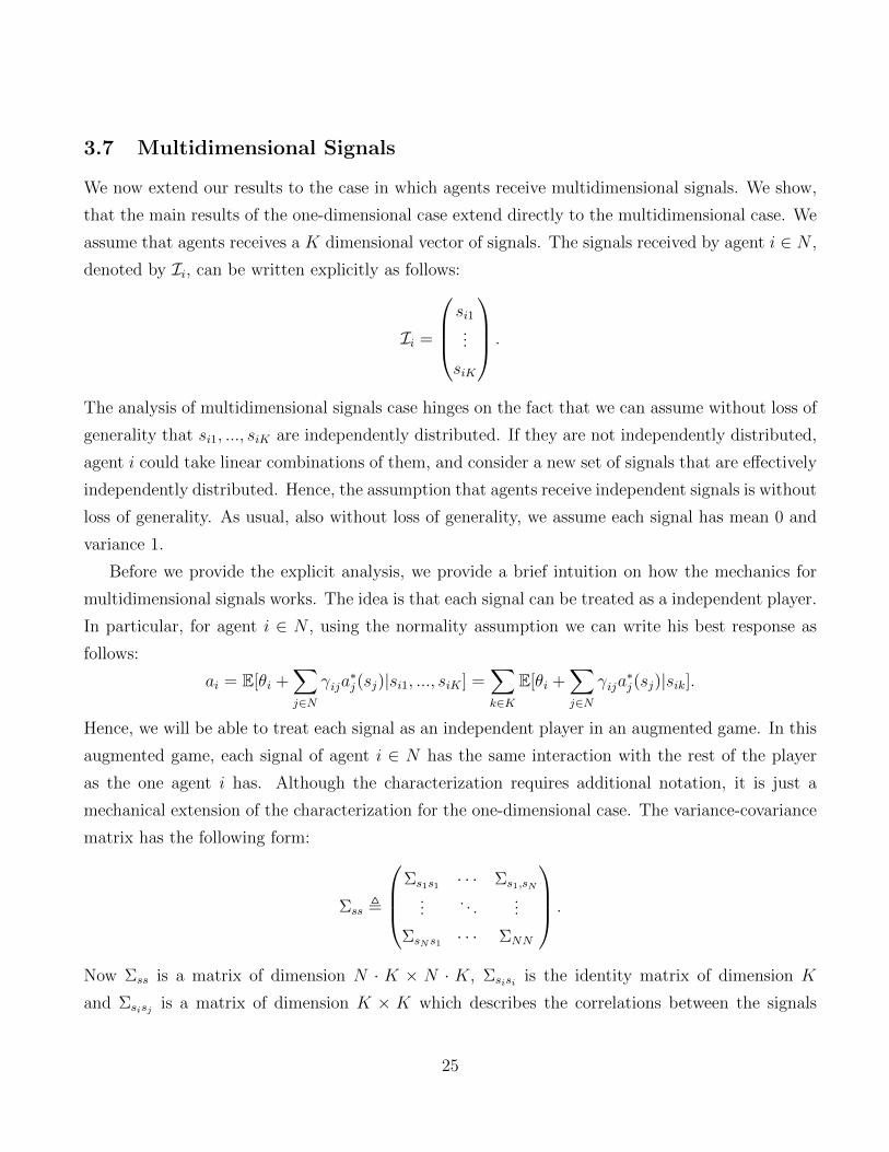
3.7 Multidimensional Signals

We now extend our results to the case in which agents receive multidimensional signals. We show,

that the main results of the one-dimensional case extend directly to the multidimensional case. We

assume that agents receives a K dimensional vector of signals. The signals received by agent i ∈ N ,

denoted by Ii, can be written explicitly as follows:

Ii =

si1...

siK

.

The analysis of multidimensional signals case hinges on the fact that we can assume without loss of

generality that si1, ..., siK are independently distributed. If they are not independently distributed,

agent i could take linear combinations of them, and consider a new set of signals that are effectively

independently distributed. Hence, the assumption that agents receive independent signals is without

loss of generality. As usual, also without loss of generality, we assume each signal has mean 0 and

variance 1.

Before we provide the explicit analysis, we provide a brief intuition on how the mechanics for

multidimensional signals works. The idea is that each signal can be treated as a independent player.

In particular, for agent i ∈ N , using the normality assumption we can write his best response as

follows:

ai = E[θi +∑j∈N

γija∗j(sj)|si1, ..., siK ] =

∑k∈K

E[θi +∑j∈N

γija∗j(sj)|sik].

Hence, we will be able to treat each signal as an independent player in an augmented game. In this

augmented game, each signal of agent i ∈ N has the same interaction with the rest of the player

as the one agent i has. Although the characterization requires additional notation, it is just a

mechanical extension of the characterization for the one-dimensional case. The variance-covariance

matrix has the following form:

Σss ,

Σs1s1 · · · Σs1,sN

.... . .

...

ΣsNs1 · · · ΣNN

.

Now Σss is a matrix of dimension N · K × N · K, Σsisi is the identity matrix of dimension K

and Σsisj is a matrix of dimension K × K which describes the correlations between the signals

25

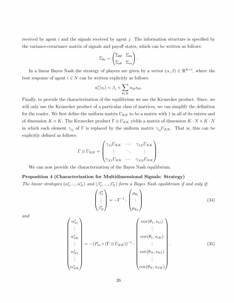
received by agent i and the signals received by agent j. The information structure is specified by

the variance-covariance matrix of signals and payoff states, which can be written as follows:

Σθs =

(Σθθ Σθs

Σsθ Σss

).

In a linear Bayes Nash the strategy of players are given by a vector (α, β) ∈ RK+1, where the

best response of agent i ∈ N can be written explicitly as follows:

a∗i (si) = βi +∑k∈K

αiksik.

Finally, to provide the characterization of the equilibrium we use the Kronecker product. Since, we

will only use the Kronecker product of a particular class of matrices, we can simplify the definition

for the reader. We first define the uniform matrix UKK to be a matrix with 1 in all of its entries and

of dimension K ×K. The Kronecker product Γ⊗UKK yields a matrix of dimension K ·N ×K ·Nin which each element γij of Γ is replaced by the uniform matrix γijUKK . That is, this can be

explicitly defined as follows:

Γ⊗ UKK =

γ11UKK · · · γ1NUKK

.... . .

...

γN1UKK · · · γNNUKK

.

We can now provide the characterization of the Bayes Nash equilibrium.

Proposition 4 (Characterization for Multidimensional Signals: Strategy)

The linear strategies (α∗1, ..., α∗N) and (β∗1, ..., β

∗N) form a Bayes Nash equilibrium if and only if:

β∗1...

β∗N

= −Γ−1 ·

µθ1

...

µθN

(34)

and

α∗11...

α∗1K...

α∗N1...

α∗NK

= −(Pss ◦ (Γ⊗ UKK))−1 ·

cov(θ1, s11)...

cov(θ1, s1K)...

cov(θN , sN1)...

cov(θN , sNK)

. (35)

26

Proposition 4 shows that equilibria can be easily computed for multidimensional singles. Al-

though the algebra becomes more tedious, it is clear the mechanics and the intuitions from the

one-dimensional case remain unchanged.

4 All Equilibrium Outcomes

4.1 Outcomes under Bayes Nash equilibrium

For any information structure a Bayes Nash equilibrium always induces a joint distribution of

actions and states (θ1, ..., θN , a1, ..., aN). Formally, for a fixed information structure, we can describe

the joint distribution of variables (θ1, ..., θN , s1, ..., sN , a∗1(s1), ..., a∗N(s2)). The joint distribution of

the first 2N variables are exogenous, while the last N variables are pin-down by the equilibrium

conditions. Now, if the analyst is not interested in the information structure that agents observe,

then it would suffice to provide the description of actions and payoff states. That is, the joint

distribution of the variables (θ1, ..., θN , a∗1(s1), ..., a∗N(s2)).

We seek to understand how the structure of the private information contributes to the behavior of

the agents, and in particular to the moments of the equilibrium distribution. Therefore, we actually

attempt to analyze the equilibrium behavior of the agents for a given description of the fundamentals

for all possible information structures. In Bergemann and Morris (2015), we considered this problem

in an abstract game theoretic setting. There we showed that a general version of Bayes correlated

equilibrium characterizes the set of outcomes that could arise in any Bayes Nash equilibrium of an

incomplete information game where agents may or may not have access to more information beyond

the given common prior over the fundamentals.

4.2 Bayes Correlated Equilibrium

We describe a Bayes correlated equilibrium in terms of the outcomes of the game, namely as a joint

distribution µ of actions (a1, ..., aN) and payoff states (θ1, ..., θN), and importantly without reference

27

to any specific information structure:

θ1

...

θN

a1

...

aN

∼ N

µθ1...

µθNµa1...

µaN

,

(Σθθ Σθa

Σθa Σaa

). (36)

Definition 2 (Bayes Correlated Equilibrium)

A joint distribution µ of variables (θ1, ..., θN , a1, ..., aN) form a Bayes correlated equilibrium if:

∀i,∀ai, Eµ[θi +∑j∈N

γijaj|ai] = 0 (37)

and the marginal distribution µ (θ) over payoff states coincide with the common prior.

As previously mentioned, the description of a Bayes correlated equilibrium makes no reference

to a information structure. Nevertheless, there is an obedience condition given by (37). This implies

that a Bayes correlated equilibrium imposes some restrictions over the set of feasible distributions of

payoff states and actions. As we see later, the fact that an agent’s action is a conditioning variable

in (37) imposes the same restrictions as agent’s observing one-dimensional signals.

4.3 Outcomes for All Information Structures

We will now characterize all joint distribution µ of actions a and payoff states θ that can be

rationalized as Bayes Nash equilibrium for some information structure.

Proposition 5 (Equivalence)

A joint distribution µ of (θ1, ..., θN , a1, ..., aN) forms a Bayes correlated equilibrium if and only if

there exists an information structure such that µ is the outcome of a Bayes Nash equilibrium.

We can now give a complete characterization of the set of Bayes correlated equilibria for a given

payoff environment (that is, a interaction structure Γ and given common prior over the payoff state

vector θ).

Proposition 6 (Characterization)

A joint distribution µ of (θ1, ..., θN , a1, ..., aN) forms a Bayes correlated equilibrium if and only if:

28

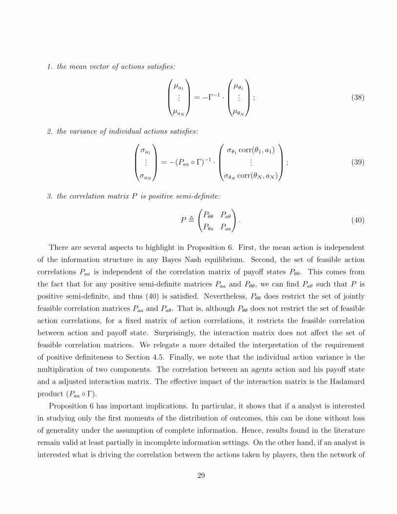
1. the mean vector of actions satisfies:µa1

...

µaN

= −Γ−1 ·

µθ1

...

µθN

; (38)

2. the variance of individual actions satisfies:σa1

...

σaN

= −(Paa ◦ Γ)−1 ·

σθ1 corr(θ1, a1)

...

σθN corr(θN , aN)

; (39)

3. the correlation matrix P is positive semi-definite:

P ,

(Pθθ Paθ

Pθa Paa

). (40)

There are several aspects to highlight in Proposition 6. First, the mean action is independent

of the information structure in any Bayes Nash equilibrium. Second, the set of feasible action

correlations Paa is independent of the correlation matrix of payoff states Pθθ. This comes from

the fact that for any positive semi-definite matrices Paa and Pθθ, we can find Paθ such that P is

positive semi-definite, and thus (40) is satisfied. Nevertheless, Pθθ does restrict the set of jointly

feasible correlation matrices Paa and Paθ. That is, although Pθθ does not restrict the set of feasible

action correlations, for a fixed matrix of action correlations, it restricts the feasible correlation

between action and payoff state. Surprisingly, the interaction matrix does not affect the set of

feasible correlation matrices. We relegate a more detailed the interpretation of the requirement

of positive definiteness to Section 4.5. Finally, we note that the individual action variance is the

multiplication of two components. The correlation between an agents action and his payoff state

and a adjusted interaction matrix. The effective impact of the interaction matrix is the Hadamard

product (Paa ◦ Γ).

Proposition 6 has important implications. In particular, it shows that if a analyst is interested

in studying only the first moments of the distribution of outcomes, this can be done without loss

of generality under the assumption of complete information. Hence, results found in the literature

remain valid at least partially in incomplete information settings. On the other hand, if an analyst is

interested what is driving the correlation between the actions taken by players, then the network of

29

strategic interactions would not be useful without further assumptions on the information structure.

Although the variance of the actions taken by players do depend on the information structure, there

is a robust prediction on how this needs to depend on the interaction structure and the equilibrium

correlation in actions.

We note that the argument here can be extended to allow for endogenous information. In

particular, in Bergemann, Heumann, and Morris (2015) we study supply function equilibria. This

equivalent to allowing agents to condition on the average action taken by other players. Although

we do not pursue the characterization for supply function equilibria any further, it is easy to extend

the results for this case. In particular, one could study models of supply function equilibria in

networks, as studied by Babus and Kondor (2014).

4.4 Role of Normality Assumption

At this point it is useful to discuss the role of normality in our analysis. This is not only useful as

it explains to what extent our results generalize to more general distributions, but it also illustrates

the arguments used in the proofs. It also provides a clear advantage of the definition of Bayes

correlated equilibrium, versus the characterization of Bayes Nash equilibrium for one-dimensional

signals.

The normality assumption makes our conditions sufficient to characterize all outcomes. To be

more specific, under the normality assumptions all outcomes are completely characterized by the

description of the first two moments of the distribution. Thus, by characterizing these two moments

we are effectively characterizing the whole distribution. Yet, for arbitrary joint distributions, con-

ditions (38) - (40) remain necessary. That is, in any Bayes Nash equilibrium (independent of the

normality assumption), the joint distribution of outcomes must satisfy (38) - (40). (38) and (39)

are a result of the linearity of the best response and the law of iterated expectation, while (40) is a

statistical property of all correlation matrices. Hence, if we pursue the exercise of characterizing all

feasible outcomes for arbitrary distributions, we would have that (38) - (40) are necessary in any

Bayes Nash equilibrium (even a non-linear one). Yet, we would also have to characterize higher

moments of the distribution to get a complete description of the set of feasible outcomes. We make

this formal in the following proposition.

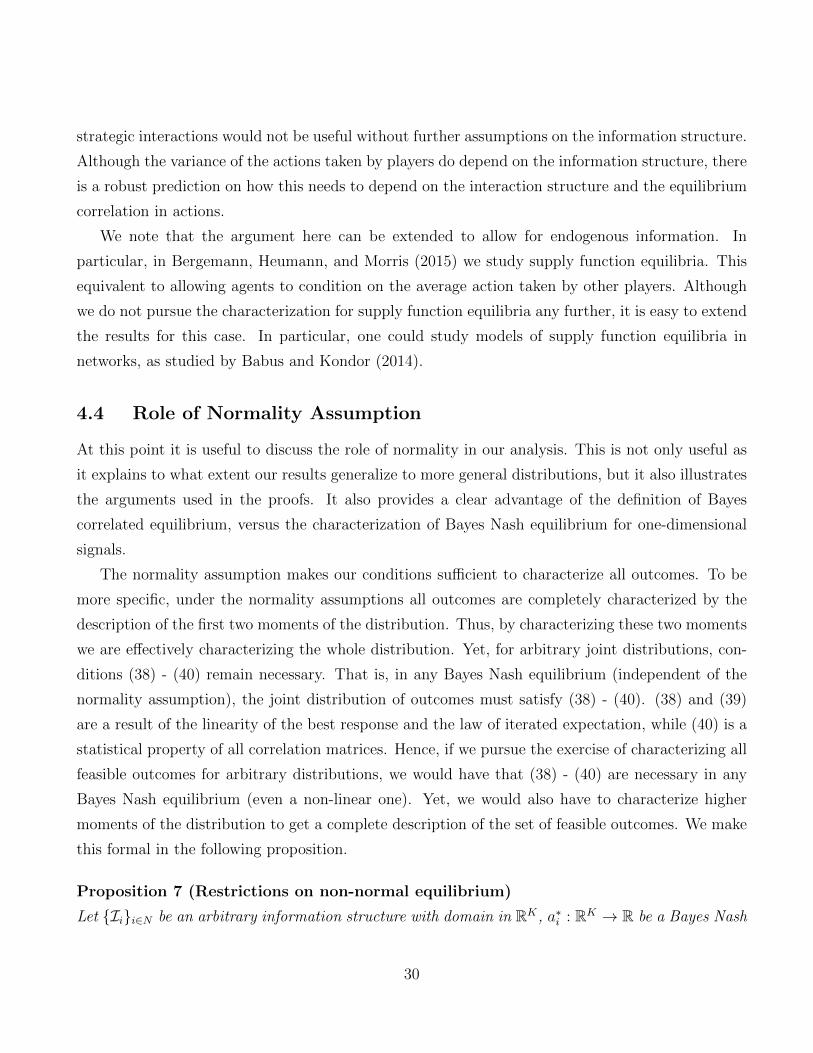
Proposition 7 (Restrictions on non-normal equilibrium)

Let {Ii}i∈N be an arbitrary information structure with domain in RK, a∗i : RK → R be a Bayes Nash

30

equilibrium and (θ1, ..., θN , a∗1, ..., a

∗N) be the outcome under this Bayes Nash equilibrium. Then, we

must have that the distribution of outcomes (θ1, ..., θN , a∗1, ..., a

∗N) satisfies (38) - (40).

Proposition 7 shows that the set of one-dimensional signals studied in Section 3 provided a

maximal description of outcomes in terms of first and second moments. That is, all possible first

and second moments that can be achieved in a BNE by some information structure, can also be

achieved when the information structure is given by one-dimensional normally distributed signals.

Although the description of Bayes correlated equilibrium extends to non-normal distributions,

the best response conditions derived in Section 3 for particular information structures does not gen-

erally hold. This comes from the fact that if we relax the normality assumption of signals, the Bayes

Nash equilibrium need not be linear in the signals received. Therefore, in a non-linear equilibrium,

the second moments do not depend only on the second moments of the signals. Moreover, for a

fixed signal structure it is necessary to characterize the whole non-linear strategy to characterize

the second moments. Hence, we can see that the characterization of a Bayes correlated equilibrium

extends more easily to non-normal information structure, while the argument used to characterize

the Bayes Nash equilibrium for normal information structures is much more restrictive.

4.5 Decomposition of Individual Volatility

We now provide a more intuitive characterization of the condition that the correlation matrix of

actions and payoff states must be positive semi-definite (that is, (40) in Proposition 6). Although

the restriction of positive semi-definiteness is imposed on P , we must take Pθθ as given, which must

be positive definite (a priori it could be positive semi-definite, but we disregard this knife edge case

for the rest of this section). The following lemma, which is a standard statistical result, will help

us provide a more intuitive characterization of the set of feasible correlation matrices for a fixed

matrix Pθθ.

Lemma 7 (Positive Definiteness)

The matrix P is positive definite if and only if Pθθ is positive definite and Paa−PaθPθθPθa is positive

definite.

Lemma 7 is useful as it characterizes the set of positive definite matrices taking as given the

correlation matrix of payoff states. It is useful to note that Paa − PaθPθθPθa is positive definite if

and only if Σaa − ΣaθΣθθΣθa is positive definite (this is called the Schur complement). Moreover,

31

for normal distributions we have:

var(

a1

...

aN

|θ1

...

θN

) = Σaa − ΣaθΣθθΣθa. (41)

Hence, a different way of expressing that P is positive definite is to say that the variance of agent’s

actions conditional on the realization of the payoff state is a well defined variance-covariance matrix.

This decomposition has a very intuitive interpretation. We can see that (41) yields how much

volatility in actions is driven by shocks that are payoff irrelevant. Alternatively, we can call this

the non-fundamental volatility.

The restriction that P must be positive definite becomes closer to bind as the non-fundamental

volatility becomes smaller. In particular, we can see that there exists a class of equilibria in which

all volatility is driven by payoff shocks.

Definition 3 (Noise Free Equilibrium)

We say a Bayes correlated equilibrium is noise free if Σaa − ΣaθΣθθΣθa = 0.

It is easy to see that for generic correlation matrices P , the Bayes correlated equilibrium will

not be noise free. Therefore, noise free equilibria can be seen as a knife edge case over all possible

correlation matrices. Nevertheless, there are natural Bayes Nash equilibria, which induce a noise

free outcome. For example, the complete information equilibrium. We should highlight though, that

the complete information equilibrium is not the only noise free equilibrium, but in fact there is a rich

class of noise free equilibria. In Bergemann, Heumann, and Morris (2015) we pursue the question

of what information structures yield the highest volatility in a symmetric environment. We show

that the equilibria that yield the maximum individual volatility, aggregate volatility and dispersion

is always in the class of noise free signals. Yet, generically it is not the complete information

equilibrium. Although we conjecture that this remains true in a heterogenous environment we have

not yet been able to prove this.

4.6 Decomposition of Aggregate Volatility

We now provide an explicit characterization of the aggregate volatility in a Bayes correlated equi-

librium. We defined earlier the average action:

a ,1

N

∑i∈N

ai,

32

and the variance of the average action is given by:

σa =1

N2

(σa1 · · · σaN

)· Paa ·

σa1...

σaN

. (42)

Although (42) reflects a simple statistical property of the variance of the average action, it allows

to illustrates what drives aggregate volatility. There are two sources that feed into the aggregate

volatility: (i) the size of individual volatility σ2ai

, and (ii) the way in which the individual actions

are aggregated statistically, which is given by Paa. In turn, we observed earlier in (39) that there

are two sources of individual volatility. First, the adjusted interaction matrix (Paa ◦Γ). Second, the

correlation between the individual action and the payoff state of an agent. By means of a simple

accounting exercise, we can then decompose the aggregate volatility into three elements which can

be understood independently:

1. The size of the individual shocks and the correlation that an agent’s action has with its own

payoff state. This is given by σθi corr(θi, ai), which is the covariance between an agents action

and his own payoff state. This affects the volatility of an individual agent’s action (as shown

in (39)). Importantly, the volatility that can arise from fundamental uncertainty increases

linearly with the size of the preference shocks σθi ;

2. The impact of the strategic interaction is given by (Paa ◦ Γ)−1 and provides the part of the

individual volatility that corresponds to the strategic interactions, which must be weighted

by the information that the agents receive (as shown in (39)).

3. The correlation in the action of the agents is given by (Paa) and aggregates the individual

actions into the average actions. It does not affect agent’s individual volatility, but rather

it affects the aggregation of the individual actions. This can be seen as this term does not

appear on (39). This is what we could call the aggregation component. Also, note that the

difference between measures of individual volatility and aggregate volatility come through this

term.

We can now understand in a common framework different sources of aggregate volatility that

papers in the literature have provided. We first discuss three papers that provide three different

explanations. Then, we discuss how one can disentangle the different explanations. Before we

33

proceed, it is worth highlighting that in all these papers the object of study is aggregate volatility

of actions. Since the objective is to understand how the aggregate volatility of actions can be large

even if payoff shocks are not correlated, all papers discussed here assume that payoff state are

independently distributed (that is, Pθθ = I).Angeletos and La’O (2013) provide a model in which informational frictions increase the cor-

relation in agents actions. The paper provides a model of pairwise interaction (that is γij = γji

and γij 6= 0 for one and only one j 6= i), and in which agents know their payoff. Although payoff

states are independently distributed, the signal agents get have a common error. This increases the

correlation between agents action, which makes the aggregate not vanish as the number of agents

goes to infinity. Thus, we can resume this mechanism by a informational friction that increases the

correlation Paa beyond what it would have been under complete information.

Acemoglu, Carvalho, Ozdaglar, and Tahbaz-Salehi (2012) provide a model of complete informa-

tion, but with heterogenous interactions. The network structure of the interactions implies that in

the complete information equilibrium the correlation of actions Paa is non-trivial. Importantly, it

is the correlation of actions that imply that the aggregate volatility does not vanish (or vanishes

slower than under the law of large numbers). Hence, we can summarize this mechanism by arguing

that the strategic interaction of agents makes the correlation of actions increase in the complete

information equilibrium.

Gabaix (2011) provide a completely different mechanism. In Gabaix (2011) it is argued that the

individual shocks of players σθi is non-uniform. In particular, it is argued (and shown empirically)

that the variance of shocks follow a power-law distribution. This implies that, even with a large

a number of player that take individual actions, there are few players that have large enough

shocks such that aggregate volatility vanishes slower than the law of large numbers. Hence, in this

mechanism the correlation in players action Paa remains independent, yet some of the individual

volatility of actions is large enough to make the aggregate volatility not vanish.

From the discussion in this paper, and the decomposition in 42, we can easily see what mecha-

nisms can be disentangles purely form observing the outcomes of the game. In particular, it is easy

to check whether individual volatility follows a power-law distribution, and hence check whether this

mechanism contributed to aggregate volatility. We should highlight that this can be measured just

by observing outcomes, and hence it is not necessary to make any assumptions on the information

structure of agents.

34

It is also easy to check whether the actions of players are correlated. Hence, it is easy to

check if this is contributing to aggregate volatility. Nevertheless, in general we can provide several

mechanisms that cause actions to be correlated.

1. Agents know their own shocks and do not care about others’ actions. In this case, the corre-

lation matrix describes the correlation structure of their shocks (given by (12) and replacing

Γ = I )

2. Shocks are independent, agents know their own shocks but they care about other actions. In

this case, the correlation matrix of actions is determination by the payoff interactions ( given

by (12) and replacing Σθθ = I ).

3. Shocks are independent, agents do not care about others actions but are uncertain of their

own shocks. In this case, the correlation matrix is determined by the information structure

(in particular, given by (17)).

Although we have provided three distinct mechanisms that cause actions to be correlated, in

general it is possible to disentangle them, at least partially.

It is easy to check whether this correlation is bigger than the one given by the individual shocks.

If this is the case, then we know that there must exist a mechanism that is increasing the correlation

in agent’s actions. If we can observe perfectly the interaction structure of agents, we can compute

the complete information equilibria. This would allow us to check whether complete information

is a reasonable assumption. Importantly, even if these correlations are consistent, this should be

considered suggestive evidence of complete information but not conclusive. This just comes from

the fact that we cannot discard that agents are getting incomplete information (in particular, one-

dimensional signals) that allows agents to play an equilibrium in which the correlation of actions is

the same than under complete information.

Finally, although purely from outcomes it is not easy to disentangle what is causing players

action to be correlated, it is easy to see how one could make such analysis more precise. If the

analyst gets more information about the information structure of agents (for example, through

surveys), then the analyst can impose additional restriction over outcomes. This allows to further

disentangle whether agent’s have enough information to play the complete information equilibria,

or it is informational frictions that is causing players actions to be correlated. We discuss how the

analyst can use additional information on the information structure agents have in Section 5.

35

4.7 Source of Aggregate Volatility

We now study how different patterns of correlations across agents can cause aggregate volatility to

not vanish. In particular, we discuss how aggregate volatility can be caused by an arbitrary large

number of shocks.

Consider a economy with a large number of agents, each of which responds to a shock. The

standard argument on why aggregate volatility should vanish as the number of agents becomes large

is a diversification argument. If each of these agents responds to a independent shocks, then the

variance of the average action should decay at a order (1/N2). As we have previously explained,

there is a large literature studying different mechanisms under which the law of large numbers does

not hold. Mechanisms provided in Angeletos and La’O (2013) and Acemoglu, Carvalho, Ozdaglar,

and Tahbaz-Salehi (2012) have emphasized different mechanisms by which single shocks can cause

aggregate volatility, even as N →∞.

We will abstract from the specific mechanisms that can cause correlation in actions, but just

study what are the properties of the correlation of actions that makes the law of large numbers

not hold. Nevertheless, for concreteness the reader may consider the following exercise. There

exists N players, and each player observes only his own payoff state. In particular, this implies

that Paa = Pθθ. Moreover, assume that the variance of each payoff state is equal to 1 (that is,

σθ1 = ... = σθN = 1). In this case, aggregate volatility is given by:

σ2a =

1

N+

1

N2

∑i∈N

∑j 6=i

ρθiθj . (43)

Although we consider the previous exercise for simplicity, it is clear that he correlation of actions

can be cause by informational frictions or strategic interactions. Yet, for the purpose of our exercise

it is irrelevant what are driving the correlation in actions.

The normality assumption ensures that we can write the individual actions in terms of in-

dependent shocks. That is, there is a vector of independent shocks (ε1, ..., εN) and parameters

{(λi1, ..., λiN)}i∈N such that the individual action is given by:

ai =∑j∈N

λijεj.

Moreover, as σai = 1, then we must have that:∑j∈N

λ2ij = 1.

36

This implies that, we can find parameters (λ1, ..., λN) such that:

a =∑j∈N

λjεj. (44)

Moreover, it is easy to see that aggregate volatility is given by:

σ2a =

∑j∈N

λ2j . (45)

Since we are assuming σai = 1, we must have that σa ≤ 1. We begin by providing a simple result

that allow us to show that in general there are no bounds on the number of shocks that drive

aggregate volatility.

Lemma 8 (Aggregate Volatility)

Let (λ1, ..., λN) be such that (45) holds, then there exists a variance-covariance matrix of actions

Σaa, with σai = 1 for all i ∈ N , such that (44) holds.

Lemma 8 shows that in general it is not possible to provide a bound on how many shocks cause

aggregate volatility. This is an interesting result, as it shows that the diversification argument does

not only fail when there is a single shock (or a fixed finite number of shocks) which causes the

aggregate volatility. We can always find a mechanism by which aggregate volatility is cause by an

arbitrary number of shocks. Even when the individual response of agents is kept normalized.

Consider first the case in which there are no strategic interactions, payoff states are independently

distributed with variance of 1 (Σθθ = I). Each agent observes a signal described as follows:

si =1

2(1 + 1√N

)(θi +

1√N

∑j∈N

θj). (46)

It is easy to check that:

E[θi|si] = (1 +1√N

)si =1

2(θi +

1√N

∑j∈N

θj).

We can now provide the aggregate volatility when agents receive signals (46) and they have a purely

predictions problem.

Lemma 9 (Aggregate Volatility No Interactions)

In the Bayes Nash equilibrium with zero interactions, independently distributed payoff states with

variance of 1 (Σθθ = I) and signals of the form (46), the average action is given by:

a =1

NE[θi|si] =

1

2(

1

N+

1√N

)∑j∈N

θj;

37

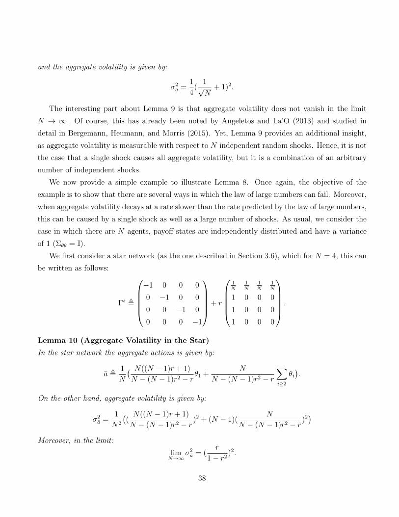
and the aggregate volatility is given by:

σ2a =

1

4(

1√N

+ 1)2.

The interesting part about Lemma 9 is that aggregate volatility does not vanish in the limit

N → ∞. Of course, this has already been noted by Angeletos and La’O (2013) and studied in

detail in Bergemann, Heumann, and Morris (2015). Yet, Lemma 9 provides an additional insight,

as aggregate volatility is measurable with respect to N independent random shocks. Hence, it is not

the case that a single shock causes all aggregate volatility, but it is a combination of an arbitrary

number of independent shocks.

We now provide a simple example to illustrate Lemma 8. Once again, the objective of the

example is to show that there are several ways in which the law of large numbers can fail. Moreover,

when aggregate volatility decays at a rate slower than the rate predicted by the law of large numbers,

this can be caused by a single shock as well as a large number of shocks. As usual, we consider the

case in which there are N agents, payoff states are independently distributed and have a variance

of 1 (Σθθ = I).We first consider a star network (as the one described in Section 3.6), which for N = 4, this can

be written as follows:

Γs ,

−1 0 0 0

0 −1 0 0

0 0 −1 0

0 0 0 −1

+ r

1N

1N

1N

1N

1 0 0 0

1 0 0 0

1 0 0 0

.

Lemma 10 (Aggregate Volatility in the Star)

In the star network the aggregate actions is given by:

a ,1

N

( N((N − 1)r + 1)

N − (N − 1)r2 − rθ1 +

N

N − (N − 1)r2 − r∑i≥2

θi).

On the other hand, aggregate volatility is given by:

σ2a =

1

N2

((N((N − 1)r + 1)

N − (N − 1)r2 − r)2 + (N − 1)(

N

N − (N − 1)r2 − r)2)

Moreover, in the limit:

limN→∞

σ2a = (

r

1− r2)2.

38

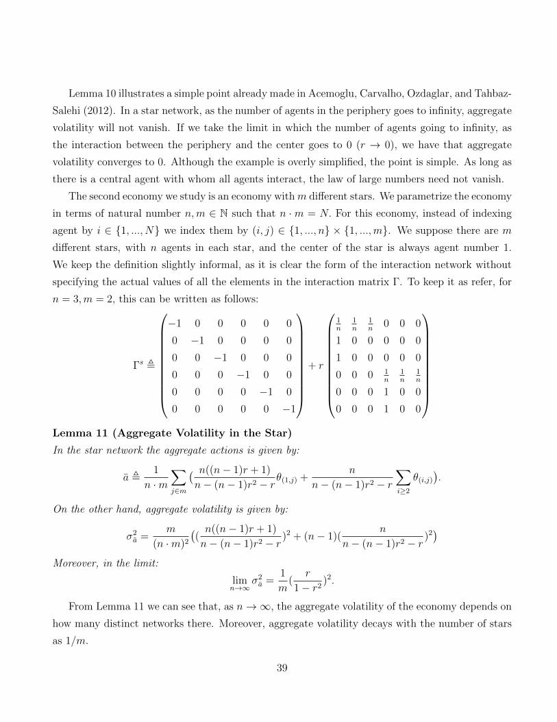
Lemma 10 illustrates a simple point already made in Acemoglu, Carvalho, Ozdaglar, and Tahbaz-

Salehi (2012). In a star network, as the number of agents in the periphery goes to infinity, aggregate

volatility will not vanish. If we take the limit in which the number of agents going to infinity, as

the interaction between the periphery and the center goes to 0 (r → 0), we have that aggregate

volatility converges to 0. Although the example is overly simplified, the point is simple. As long as

there is a central agent with whom all agents interact, the law of large numbers need not vanish.

The second economy we study is an economy withm different stars. We parametrize the economy

in terms of natural number n,m ∈ N such that n ·m = N. For this economy, instead of indexing

agent by i ∈ {1, ..., N} we index them by (i, j) ∈ {1, ..., n} × {1, ...,m}. We suppose there are m

different stars, with n agents in each star, and the center of the star is always agent number 1.

We keep the definition slightly informal, as it is clear the form of the interaction network without

specifying the actual values of all the elements in the interaction matrix Γ. To keep it as refer, for

n = 3,m = 2, this can be written as follows:

Γs ,

−1 0 0 0 0 0

0 −1 0 0 0 0

0 0 −1 0 0 0

0 0 0 −1 0 0

0 0 0 0 −1 0

0 0 0 0 0 −1

+ r

1n

1n

1n

0 0 0

1 0 0 0 0 0

1 0 0 0 0 0

0 0 0 1n

1n

1n

0 0 0 1 0 0

0 0 0 1 0 0

Lemma 11 (Aggregate Volatility in the Star)

In the star network the aggregate actions is given by:

a ,1

n ·m∑j∈m

( n((n− 1)r + 1)

n− (n− 1)r2 − rθ(1,j) +

n

n− (n− 1)r2 − r∑i≥2

θ(i,j)

).

On the other hand, aggregate volatility is given by:

σ2a =

m

(n ·m)2

((n((n− 1)r + 1)

n− (n− 1)r2 − r)2 + (n− 1)(

n

n− (n− 1)r2 − r)2)

Moreover, in the limit:

limn→∞

σ2a =

1

m(

r

1− r2)2.

From Lemma 11 we can see that, as n→∞, the aggregate volatility of the economy depends on

how many distinct networks there. Moreover, aggregate volatility decays with the number of stars

as 1/m.

39

If we contrast Lemma 9 with Lemma 11 we can identify two distinct ways in which the law of

large numbers may fail to hold. First, if the economy has a central agent, as in the unique star

network, then aggregate volatility will decay as the importance of the center agent becomes smaller.

In these situations, aggregate volatility may converge at a rate slower than 1/N as the importance

of the shock to the center agent decays slower. Importantly, we can identify a single shock that

cause aggregate volatility not to decay.

On the other hand, from Lemma 11 we can identify a different mechanism. It is possible that

the importance of the center within clusters does not becomes smaller, but it is the number of

clusters that become bigger (that is, a larger m). In this case, aggregate volatility will decay with

the number of clusters. Importantly, in this case it would be impossible to identify a single shock

causing aggregate volatility, but it would be a large number of shocks that cause aggregate volatility

to vanish slowly. Of course, we could take limits in a unique star network and in a network with

many stars and have the same rate of decay of aggregate volatility, but with very different patterns

on the number of shocks causing aggregate volatility.

5 Additional Informational Restrictions

A Bayes correlated equilibrium provides us with a general characterization of all feasible outcomes.

Yet, it is often the analyst can impose restrictions on the information agents have. That is, the

analyst knows that agent i has access at least to a signal si, where the joint distribution of signals

and payoff states is normally distributed and given by (5). If the analyst knew that agents get signals

(s1, ..., sN) and nothing else beyond these signals, then the analyst could compute the equilibrium

by just computing the Bayes Nash equilibrium of the game. Yet, it may be the case that the

analyst cannot impose any additional restriction on the information set of agents beyond the fact

that agents know signals (s1, ..., sN). In particular, on what information they may have in addition

to these signals.

Since we assume the analyst knows that agents can see signals (s1, ..., sN), we are implicitly

assuming that the analyst can observe the realization of this signals. Hence, whenever we refer to an

outcome in this section we will refer to the joint distribution of variables (θ1, ..., θN , a1, ..., aN , s1, ..., sN).

We now characterize all feasible outcomes in which players know at least signals (s1, ..., sN). The

argument follows similar lines as the one in which no informational assumptions were made, but in

this case we directly define and solve for the adequate Bayes correlated equilibrium. It will become

40

clear that the argument follows similar lines.

Definition 4 (Bayes Correlated Equilibrium with Informational Restrictions.)

A joint distribution µ of (θ1, ..., θN , a1, ..., aN , s1, ..., sN) forms a Bayes correlated equilibrium with

informational restrictions if:

∀i, ∀ai, Eµ[θi +∑j∈N

γijaj|ai, si] = 0 (47)

and the marginal distribution µ (θ) over payoff states coincide with the common prior.

The definition of Bayes correlated equilibrium follows similar lines as the one in Definition 2.

Nevertheless, we have augmented the outcome space to allow for the additional information that

the analyst can observe. In this case, the analyst has more information on the information agents

have. The analyst observes directly (s1, ..., sN), but also observe the agents actions. As the reader

might expect, this will provide a description of all outcomes when agents know at least (s1, ..., sN).

We make this formal in the following propositions.

Proposition 8 (Equivalence under Informational Restrictions)

A joint distribution µ of (θ1, ..., θN , a1, ..., aN , s1, ..., sN) forms a Bayes correlated equilibrium if and

only if there exists an information structure in which agent i ∈ N knows si, such that µ is the

outcome of a Bayes Nash equilibrium.

We can see that with the adequate adjustment in the definition we can accommodate models in

which the analyst has some information about the information structure of agents. Moreover, as we

show in the following lemma, the characterization remains tractable. Moreover, as we discuss later,

the additional information that the analyst has on the information structure allows the analyst to

restrict the set of feasible outcomes in interesting ways.

Proposition 9 (Characterization under Informational Constraints)

A joint distribution µ of (θ1, ..., θN , a1, ..., aN , s1, ..., sN) forms a Bayes correlated equilibrium in

which agents know at least s if and only if:

1. the mean vector of actions satisfies:µa1

...

µaN

= −Γ−1 ·

µθ1

...

µθN

; (48)

41

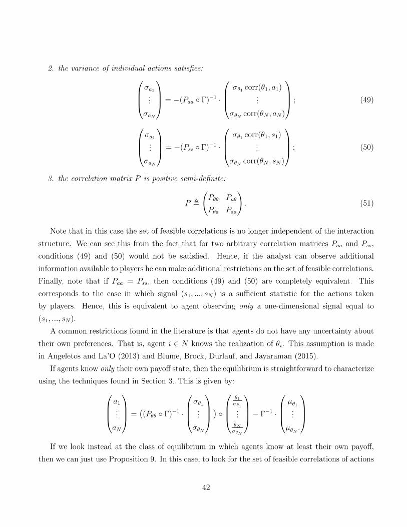
2. the variance of individual actions satisfies:σa1

...

σaN

= −(Paa ◦ Γ)−1 ·

σθ1 corr(θ1, a1)

...

σθN corr(θN , aN)

; (49)

σa1

...

σaN

= −(Pss ◦ Γ)−1 ·

σθ1 corr(θ1, s1)

...

σθN corr(θN , sN)

; (50)

3. the correlation matrix P is positive semi-definite:

P ,

(Pθθ Paθ

Pθa Paa

). (51)

Note that in this case the set of feasible correlations is no longer independent of the interaction

structure. We can see this from the fact that for two arbitrary correlation matrices Paa and Pss,

conditions (49) and (50) would not be satisfied. Hence, if the analyst can observe additional

information available to players he can make additional restrictions on the set of feasible correlations.

Finally, note that if Paa = Pss, then conditions (49) and (50) are completely equivalent. This

corresponds to the case in which signal (s1, ..., sN) is a sufficient statistic for the actions taken

by players. Hence, this is equivalent to agent observing only a one-dimensional signal equal to

(s1, ..., sN).

A common restrictions found in the literature is that agents do not have any uncertainty about

their own preferences. That is, agent i ∈ N knows the realization of θi. This assumption is made

in Angeletos and La’O (2013) and Blume, Brock, Durlauf, and Jayaraman (2015).

If agents know only their own payoff state, then the equilibrium is straightforward to characterize

using the techniques found in Section 3. This is given by:a1

...

aN

=((Pθθ ◦ Γ)−1 ·

σθ1...

σθN

) ◦

θ1σθ1...θNσθN

− Γ−1 ·

µθ1...

µθN .

If we look instead at the class of equilibrium in which agents know at least their own payoff,

then we can just use Proposition 9. In this case, to look for the set of feasible correlations of actions

42

we need to look for Paa such that:

(Paa ◦ Γ)−1 ·

σθ1 corr(θ1, a1)

...

σθN corr(θN , aN)

= (Pθθ ◦ Γ)−1 ·

σθ1 corr(θ1, s1)

...

σθN corr(θN , sN)

. (52)

We can see that this imposes additional restrictions on Paa beyond the requirement of positive

definiteness. Yet, it is clearly not uniquely pin down by (52). Heuristically, we can see this by

noting Paa have (N − 1)(N − 2)/2 independent variables (all correlations), while (52) constitutes

only N different equations. Of course, a solution is Paa = Pθθ which corresponds to agents knowing

only their own payoff state.

6 Conclusions

We studied a model of linear interactions with heterogeneous interactions, heterogenous incomplete

information and heterogeneous payoff shocks. We provided a class of one-dimensional signals that

allow to span all first and second moments of the outcome in any Bayes Nash equilibrium. Moreover,

we provided a very tractable characterization of the linear Bayes Nash equilibrium for these class

of signals. Our results apply and provide novel insights in a variety of different applications.

7 Appendix

Throughout the appendix, we use the following lemma.

Lemma 12 (Characterization of Expectations)

Let (x, y, z1, ..., zJ) be a joint distribution of variables such that x = E[y|z1, ..., zJ ], then

∀j ∈ J, cov(x, zj) = cov(y, zj) ; σ2x = cov(x, y) and E[x] = E[y]. (53)

On the other hand, if (x, y, z1, ..., zJ) is a jointly normal distribution of variables such that x is

measurable with respect to (z1, ..., zJ) and (53) is satisfied, then x = E[y|z1, ..., zJ ].

43

Proof of Lemma 1. Using the law of iterated expectations:

E[a∗i (si)(θi +∑j∈N

a∗j(sj)−γii2a∗i (si))] = E[E[a∗i (si)(θi +

∑j∈N

a∗j(sj)−γii2a∗i (si))|a∗i (si)]]

= E[a∗i (si)E[θi +∑j∈N

a∗j(sj)|a∗i (si)]−γii2

(a∗i (si))2]

= E[γii2

(a∗i (si))2] =

γii2

(σ2ai

+ µ2ai

).

where we use that E[a∗i (si)E[θi +∑

j∈N a∗j(sj)|a∗i (si)] = 0 by 7. Hence, we get the result. �

Proof of Proposition 1. Using Lemma 12, we know that (where we use that si has mean of 0):

E[∑j∈N

γij(α∗jsj + β∗j) + θi|si] = 0 ⇐⇒

∑j∈N

γijβ∗j + µθi = 0 and

∑j∈N

γijα∗jcov(sj, si) + cov(θi, si) = 0.

We now show that (13) and (14) are equivalent to:

∀i ∈ N,∑j∈N

γijβ∗j + µθi = 0 and

∑j∈N

γijα∗jcov(sj, si) + cov(θi, si) = 0.

We can immediately check that: β∗1...

β∗N

= −Γ−1

µ∗θ1...

µ∗θN

.

Using that si has a variance of 1, we can write the condition on α∗i as follows:∑j∈N

γijα∗jρsjsi + cov(θi, si) = 0.

Writing it in matrix form, we get:

Γ ·

α∗1...

α∗N

=

cov(s1, θ1)

...

cov(sN , θN)

.

Hence, we get the result.�

Proof of Proposition 2. In a linear Bayes Nash equilibrium we have that:

a∗i (si) = β∗i + α∗i si.

Since by assumption signals have 0 mean, we have that:

E[a∗i (si)] = β∗i .

44

Looking at the characterization of (β∗1, ..., β∗N), we clearly get (15). On the other hand, as signals

have a variance of 1, we have that:

σai = α∗i .

Looking at the characterization of (α∗1, ..., α∗N), we clearly get (16). Finally, as a∗i (si) is a linear

function of si, we have that the correlation matrix of the variables (θ1, ..., θN , s1, ..., sN) is the same

as the correlation matrix of (θ1, ..., θN , a∗1(s1), ..., a∗N(sN)). Hence, we get (17). �

Proof Proposition 5 (Only If) Let µ be a joint distribution of (θ1, ..., θN , a1, ..., aN) that forms a

Bayes correlated equilibrium. Now consider a information structure in which agent i ∈ N receives

a one dimensional signal si, where the joint distribution of (θ1, ..., θN , s1, ..., sN) is the same as the

distribution of (θ1, ..., θN , a1, ..., aN). Now consider the following strategy profile a∗i : R→ R,

∀i ∈ N, a∗i (si) = si.

Since, µ forms a Bayes correlated equilibrium, and the joint distribution of (θ1, ..., θN , s1, ..., sN) is

the same as the distribution of (θ1, ..., θN , a1, ..., aN) we have that:

∀i ∈ N, E[θi +∑j∈N

γijaj|ai] = E[θi +∑j∈N

γijsj|si] = E[θi +∑j∈N

γija∗j(sj)|si] = 0

Hence, {a∗i }i∈N forms a Bayes Nash equilibrium when agents receive information structure (θ1, ..., θN , s1, ..., sN).

Trivially, we have that the joint distribution of (θ1, ..., θN , a∗1(s1), ..., a∗N(sN)) is the same as the dis-

tribution of (θ1, ..., θN , a1, ..., aN).

(If) Consider some information structure {Ii}i∈N and let µ be the distribution over outcomes

(θ1, ..., θN , a∗1(I1), ..., a∗N(IN)) induced by the Bayes Nash equilibrium. By the definition of a Bayes

Nash equilibrium:

∀i ∈ N, E[θi +∑j∈N

γija∗j(Ij)|Ii] = 0.

We know that a∗i (Ii) is measurable with respect to Ii. Hence,

∀i ∈ N, E[θi +∑j∈N

γija∗j(Ij)|Ii, a∗i (Ii)] = 0.

By taking expectations of the previous equation and using the law of iterated expectations:

∀i ∈ N, E[E[θi +∑j∈N

γija∗j(Ij)|Ii, a∗i (Ii)]|a∗i (Ii)] = E[θi +

∑j∈N

γija∗j(Ij)|a∗i (Ii)] = E[0|a∗i (Ii)] = 0.

45

Hence, we have that:

∀i ∈ N, E[θi +∑j∈N

γija∗j(Ij)|a∗i (Ii)] = 0.

Hence, the joint distribution over (θ1, ..., θN , a∗1(I1), ..., a∗N(IN)) forms a Bayes correlated equilib-

rium.

Hence, we prove the result. �

Proof Proposition 6 (Only If) Let µ be a joint distribution of (θ1, ..., θN , a1, ..., aN) that forms a

Bayes correlated equilibrium. The correlation matrix of (θ1, ..., θN , a1, ..., aN) must be positive semi-

definite to be a valid correlation matrix. Hence (40) is trivially satisfied. Moreover, by definition of

a Bayes correlated equilibrium:

∀i ∈ N, E[θi +∑j∈N

γijaj|ai] = 0. (54)

By taking expectations, and using the law of iterated expectations, we get:

∀i ∈ N, µθi +∑j∈N

γijµaj = 0. (55)

It is easy to check that (38) corresponds to the matrix representation of 55. By multiplying (54)

by ai, taking expectations and using the law of iterated expectations:

∀i ∈ N, E[θiai] +∑j∈N

γijE[aiaj] = 0.

We can rewrite the equation as follows:

∀i ∈ N, cov(θi, ai) + µθiµai +∑j∈N

γij(cov(ai, aj) + µaiµaj) = 0.

Using (55), we get:

∀i ∈ N, cov(θi, ai) +∑j∈N

γijcov(ai, aj) = 0.

By definition of a covariance, we have:

∀i ∈ N, ρθi,aiσθiσai +∑j∈N

γijρaiajσajσai = 0. (56)

It is easy to check that (39) is the matrix representation of (56).

46

(If) Let µ be a joint distribution of (θ1, ..., θN , a1, ..., aN) satisfying (38) and (39) ((40) is trivially

satisfied). Rewriting the equations we have that:

∀i ∈ N, µθi +∑j∈N

γijµaj = 0;

∀i ∈ N, cov(θi, ai) +∑j∈N

γijcov(ai, aj) = 0.

Using Lemma ??, we have that:

µθi +∑j∈N

γijµaj = 0 and cov(θi, ai) +∑j∈N

γijcov(ai, aj) = 0⇒ E[θi +∑j∈N

γijaj|ai] = 0.

Hence,

∀i ∈ N, E[θi +∑j∈N

γijaj|ai] = 0.

Hence, the joint distribution of (θ1, ..., θN , a1, ..., aN) forms a Bayes correlated equilibrium.

Hence, we prove the result. �

Proof Proposition 7 Let (I1, ..., IN) be an arbitrary information structure. Using the same

definition for Bayes Nash equilibrium as Definition 1, we must have that:

∀i ∈ N, E[θi +∑j∈N

γija∗j(Ij)|Ii] = 0. (57)

Using the law of iterated expectations, we get:

∀i ∈ N, µθi +∑j∈N

γijµaj = 0. (58)

Hence, we get (15). Additionally, we know that a∗i (Ii) is measurable with respect to Ii. Multiplying

(57) by a∗i (Ii) and taking expectations, we get:

∀i ∈ N, E[a∗i (Ii)θi] +∑j∈N

γijE[a∗i (Ii)a∗j(Ii)] = 0. (59)

Using (59), we get:

∀i ∈ N, cov(ai, θi) +∑j∈N

γijcov(ai, aj) = 0. (60)

Writing this in matrix form, we get (16). �

Proof Lemma 12 We refer to the first part of the statement as the “only if” part and the second

part of the statement as the “if” part.

47

(Only If). Let x be defined as follows:

x = E[y|z1, ..., zJ ].

Taking expectations of the previous equation we get:

E[x] = E[y]. (61)

Multiplying the previous equation by zj and taking expectations, we get:

E[xzj] = E[yzj].

Using (61) we get:

cov(x, zj) = cov(y, zj).

Similarly, we get:

σ2x = cov(y, x).

Hence, we get that the conditions are necessary.

(If). Let x be defined as follows:

x = E[y|z1, ..., zJ ].

We will show that the joint distribution of (x, y, z1, ..., zJ) is the same as the joint distribution of

(x, y, z1, ..., zJ) and hence x = E[y|z1, ..., zJ ]. Since all random vectors are normal, then we have

that the joint distribution is completely determined by the first and the second moments.

It is easy to see that E[x] = E[x]. Using the first part of the proof, it is also easy to see that:

∀j ∈ J, cov(x, zj) = cov(y, zj) = cov(x, zj). (62)

By definition x is measurable with respect to (z1, ..., zJ) and by assumption x is measurable with

respect to (z1, ..., zJ). Hence,

var(x|z1, ..., zJ) = var(x|z1, ..., zJ). (63)

Using (62), (62) and standard results for normal distributions:

σ2x = σ2

x.

Finally, once again, using the first part of the proof, it is also easy to see that:

cov(x, y) = σ2x = σ2

x = cov(x, y). (64)

Hence, the joint distribution of variables(x, y, z1, ..., zJ) is the same as the joint distribution of

(x, y, z1, ..., zJ). Hence, we get the result. �

48

References

Acemoglu, D., V. Carvalho, A. Ozdaglar, and A. Tahbaz-Salehi (2012): “The Network

Origins of Aggregate Fluctuations,” Econometrica, 80, 1977–2016.

Angeletos, G.-M., and J. La’O (2013): “Sentiments,” Econometrica, 81, 739–779.

Babus, A., and P. Kondor (2014): “Trading and Information Diffusion in Over-the-Counter

Markets,” Discussion paper, Federal Reserve Bank of Chicago and Central European University.

Ballester, C., A. Calvo-Armengol, and Y. Zenou (2006): “Who’s Who in Networks.

Wanted: The Key Player,” Econometrica, 74, 1403–1417.

Bergemann, D., T. Heumann, and S. Morris (2015): “Information and Volatility,” Journal

of Economic Theory, forthcoming.

Bergemann, D., and S. Morris (2013): “Robust Predictions in Games with Incomplete Infor-

mation,” Econometrica, 81, 1251–1308.

Bergemann, D., and S. Morris (2015): “Bayes Correlated Equilibrium and the Comparison of

Information Structures in Games,” Theoretical Economics, forthcoming.

Blume, L., W. Brock, S. Durlauf, and R. Jayaraman (2015): “Linear Social Interaction

Models,” Journal of Political Economy, 123, 444–496.

Calvo-Armengol, A., and J. de Marti (2009): “Information Gathering in Organizations:

Equilibrium, Welfare and Optimal Network Structure,” Journal of the European Economic As-

sociation, 7(116-161).

Calvo-Armengol, A., J. de Marti, and A. Prat (2015): “Communication and Influence,”

Theoretical Economics, forthcoming.

de Marti, J., and Y. Zenou (2013): “Network Games with Incomplete Information,” Stockholm

University.

Gabaix, X. (2011): “The Granular Origins of Aggregate Fluctuations,” Econometrica, 79, 733–

772.

49

Morris, S. (1997): “Interaction Games: A Unified Analysis of Incomplete Information, Local

Interaction and Random Matching Games,” Discussion Paper http://ssrn.com/abstract=290880,

Department of Economics, Princeton University.

Morris, S., and H. Shin (2002): “Social Value of Public Information,” American Economic

Review, 92, 1521–1534.

50