A CHARACTERIZATION FOR OPTIMAL BUNDLING OF PRODUCTS WITH INTER-DEPENDENT VALUES

By

Soheil Ghili

February 2021

COWLES FOUNDATION DISCUSSION PAPER NO. 2273

COWLES FOUNDATION FOR RESEARCH IN ECONOMICS YALE UNIVERSITY

Box 208281 New Haven, Connecticut 06520-8281

http://cowles.yale.edu/

A Characterization for Optimal Bundling of Products

with Inter-dependent Values

Soheil Ghili∗

Yale University

February 26, 2021

Abstract

This paper studies optimal bundling of products with inter-dependent values. I

show that, under some conditions, a firm optimally chooses to sell only the full bundle

of a given set of products if and only if the optimal sales volume of the full bundle

is larger than the optimal sales volume for any smaller bundle. I then provide an

interpretation of this characterization based on (i) the magnitude of the variation

across consumers in how complementary they find different products, and (ii) how this

variation correlates with price sensitivity.

1 Introduction

This paper has two objectives. First, I characterize necessary and sufficient conditions for

when pure bundling of a finite number of products with inter-dependent values is optimal

for a monopolist. Second I provide an interpretation of this characterization and examine

the relevance and usefulness of that interpretation using simulation.

The literature on theoretical analysis of optimal bundling decisions is large and growing.

To my knowledge, however, there has not been a full characterization of when it is optimal to

bundle. This paper provides such characterization for “pure” bundling (i.e., the act of selling

only the package of all available products together as one bundle). Under some assumptions,

most notably weak complementarity across products and a form of vertical differentiation

∗E-mail: soheil.ghili@yale.edu. Click here for the most current version.

1

among potential consumers, I prove that optimal bundling admits a simple characterization:

Pure bundling is optimal if the optimal sales volume for the full bundle (if sold alone) is

strictly larger than that for any other bundle. Conversely, if there is at least one bundle

whose optimal sales volume (if sold alone) is strictly larger than that of the full bundle, then

pure bundling is sub-optimal.1 In simpler terms, bundling is optimal if it helps sell more.

The simplicity of this characterization and its tight conditions provide an opportunity

to arrive at useful interpretations. I argue that this result has two implications. First,

the variation across consumers in the complementarity levels among products is important

for bundling decisions. The more such variation, the more likely it is for unbunbling to be

optimal. Second, I argue that it is not just the magnitude of the variation in complementarity

that matters. It also matters how correlated this variation across consumers is with the

variation in price sensitivity. If more price sensitive consumers see more complementarity

across products, then the optimality of bundling becomes more likely. Variants of this latter

interpretation were previously mentioned in the literature. As such, in discussing it, I do

not rely only on the characterization in this paper; I also draw on results and interpretations

by Long (1984); Armstrong (2013) on the comparison between the price elasticity demand

for the full bundle and those of individual products, as well as by Haghpanah and Hartline

(2019) on the monotonicity of the ratio between the valuations of sub-bundles and that

of the full bundle in the valuation of the full bundle itself. I show the relevance of these

two interpretations for applied work using a simulation of random-coefficient discrete choice

demand models a la Berry et al. (1995).

The rest of the paper is organized as follows. Section 2 reviews the related literature.

Section 3 sets up the model, presents the characterization of optimal bundling decisions, and

discusses its relation to other results in the literature. Section 4 discusses the interpretation

of the main result. Section 5 showcases the relevance of the interpretation for applied work

using a simulation. Section 6 concludes.

1Note that this is slightly short of a full characterization given it does not determine the optimal bundlingstrategy when the optimal sales volume for the full bundle is larger than those for some smaller bundles butexactly equal to some others. It can be shown that a strengthening of my model assumptions will implyfull bundling is optimal in this case, completing the if-and-only-if characterization. Nevertheless, I see thebenefit from being able to speak to this special scenario as too marginal to justify the stronger assumptionsit requires. As such, I maintain the smaller set of assumptions that do not speak to this special case. Seesection 3 for more details.

2

2 Related Literature

The study of bundling has a large literature which dates at least as far back as Stigler

(1963). The majority of the papers in this literature focus on the case of “independent

values,” meaning the valuation by each consumer of any given product i is not impacted by

whether she also possesses product i′ 6= i. Pioneering in this area was Adams and Yellen

(1976), pointing out that bundling can be more profitable than unbundling when there is

negative correlation among consumers in how they value individual products. Other studies

such as McAfee et al. (1989); Menicucci et al. (2015); Pavlov (2011); Schmalensee (1984);

Fang and Norman (2006) further develop results on optimal bundling under independent

values. Most of these studies concentrate on sufficient conditions for bundling and many

focus on a setting with two products only. Although most of this literature examines a

monopolist seller (which is also the focus of this paper), some studies have analyzed multiple

sellers (McAfee et al. (1989); Zhou (2017, 2019)).

The literature allowing for dependence in product valuations, to which this paper belongs,

is considerably smaller. Part of this literature focuses directly on bundling (e.g., Haghpanah

and Hartline (2019); Armstrong (2013, 2016); Long (1984)) whereas some study price discrim-

ination settings which have implications for bundling (e.g., Anderson and Dana Jr (2009);

Deneckere and Preston McAfee (1996)). This paper complements this literature in that it

imposes a different set of assumptions (stronger only than those imposed by Haghpanah

and Hartline (2019)) and delivers simple but necessary and sufficient conditions for bundling

based on optimal quantities sold. I also contribute to this sub-literature in two other ways.

First, by connecting the interpretation of my results to those based on price elasticities (such

as Long (1984); Armstrong (2013)) and those based on ratio monotonicity (such as Hagh-

panah and Hartline (2019); Anderson and Dana Jr (2009); Deneckere and Preston McAfee

(1996); Salant (1989)), I also illuminate the relationship between the intuitions from these

two sets of results themselves, a connection not made before. Second, to my knowledge, this

paper makes the first attempt to take insights from the analysis of optimal bundling under

inter-dependent values to applied models of demand.

3

3 Model

3.1 Setup

There are n products indexed 1 through n. Possible bundles of these products are denoted

b ⊆ {1, ..., n}. Set B = {b|b ⊆ {1, ..., n}} represents the set of all possible bundles.2 By

b denote the full bundle {1, ..., n}. There is a unit mass of customers whose types are

represented by t with probability distribution f(·) > 0. The willingness to pay by type t for

bundle b is denoted v(b, t). Without loss, assume v(∅, t) = 0.

The problem the firm solves has two components. First, the firm makes a bundling

decision. It chooses the optimal set B∗ of bundles b among subsets B of B that satisfy ∅ /∈ B.

Note that there are as many as 22n−1 possible bundling strategies. Thus, characterizing the

conditions under which the firm can simply choose B∗ = {b} should indeed be of value.

The second decision by the firm is choosing prices p(·) : B → R for the bundles offered.3

Denote by PB the set of all possible such pricing functions.

Once the firm has decided on set B and prices p(·), customers decide which bundles to

purchase. Each customer t’s decision β(t|B, p) ⊆ B is determined by:

β(t|B, p) = arg maxβ⊆B

v(∪b∈βb, t)− Σb∈βp(b) (1)

Throughout the paper, I assume customers break ties in favor of more expensive bundles

and randomize evenly if similarly priced bundles tie for first. Also, note that equation 1

implies that customers want at most one unit of each product i and find additional units

redundant.

Demand for bundle b is given by the measure of customers t who would choose to purchase

bundle b:

D(b|B, p) =

∫t

1b∈β(t|B,p)f(t)dt (2)

Firm profit under bundling strategy B and pricing strategy p is given by:

π(B, p) = Σb∈BD(b|B, p)(p(b)− Σi∈bci

)(3)

2My notation, in part, follows Haghpanah and Hartline (2019).3Note that, in principle, one could model the bundling decision through pricing; because not offering a

product would be equivalent to pricing it so high that no customer would purchase it. As such, separatingthe bundling and pricing decisions in the model is, in some sense, redundant. Nevertheless, I decided tocarry out this separation because it provides a more streamlined notation for the problem.

4

where ci is the (constant) marginal cost of producing a unit of good i. Costs ci can be

negative, allowsing for “damaged-good” settings a la Deneckere and Preston McAfee (1996).

We can now write out the firm’s problem. The firm optimally chooses B∗ and p∗ maximize

profit:

(B∗, p∗) = arg maxB∈B,p∈PB

π(B, p) (4)

With the setup of the firm problem laid out, I now introduce a few more definitions and

notations. For any disjoint bundles b and b′, denote by v(b, t|b′) the valuation by type t for

b conditional on possessing b′. Formally:

v(b, t|b′) ≡ v(b ∪ b′, t)− v(b′, t)

In a similar manner, denote β(t|B, p, b′) = arg maxβ⊆(B\{b′}) v(∪b∈βb, t|b′)−Σb∈βp(b). Also

denote D(b|B, p, b′) =∫t1b∈β(t|B,p,b′)f(t)dt. Finally, denote

π(B, p|b′) = Σb∈B\{b′}D(b|B, p, b′)(p(b)− Σi∈bci

).

Finally, at times with some abuse of notation I will refer to ∪b∈β(t|B,p,b′)b simply by

β(t|B, p, b′). I next turn to the assumptions and the main result.

3.2 Main Result

The main results of the paper is about how optimal bundling decisions are informed by the

comparison among optimal sales volumes for different bundles. I start with some necessary

assumptions and definitions.

Assumption 1. Monotonicity: Consider t and t′ such that v(b, t) > v(b, t′). Then for all

disjoint b and b′, we have v(b, t|b′) > v(b, t′|b′).4

Assumption 2. Complementarity: For any type t and disjoint bundles b and b′, we have:

v(b ∪ b′, t) ≥ v(b, t) + v(b′, t)

4The strict inequality in v(b, t|b′) > v(b, t′|b′) is not necessary for the proof of the main result; the weakversion v(b, t|b′) ≥ v(b, t′|b′) would suffice. Nevertheless, I decided to use the strict version as it simplifiesthe notations for the proof substantially.

5

Assumption 3. Quasi-concavity: For any b ∈ B, profit function π(B, p|b′) is strictly

quasiconcave in p(b) for all values of p(b) that yield strictly positive demand for b.5

Assumption 4. Non-triviality: for every product i ∈ {1, ..., n}, there is a non-measure-

zero set of types t such that v({i}, t) > ci.

Assumption 5. Continuity: for any bundle b, value function v(b, t) has at most finitely

many points where it is discontinuous in t.

Definition 1. By D∗(b) denote the “optimal quantity sold” of bundle b if no other bundle

were offered by the firm. Formally, D∗(b) is defined as D(b|{b}, p∗b) where p∗b is the optimal

price for bundle b when B = {b}.

Definition 2. A given firm strategy (B, p) involves pure bundling if for any customer of

type t, we have:

∪b∈β(t|B,p)b ∈ {∅, b}

This definition for pure bundling is “neat” in the sense that it avoids some technical issues.

For instance, if B includes bundles other than b but at prices so high that no customer would

purchase them, Definition 2 considers it pure bundling. In a similar vein, if under (B, p)

multiple bundles are offered but the prices are such that each customer who buys anything

combines them to construct b, then this definition again detects pure bundling. One can

verify that whenever the conditions in this definition hold, it is (not necessarily uniquely)

optimal for the firm to offer only the full bundle B = {b}. With this definition, we are now

ready to state the main result.

Theorem 1. Under assumptions 1 through 5, the optimal strategy (B∗, p∗) involves pure

bundling if:

D∗(b) > maxb∈B\{b}

D∗(b)

Conversely, the optimal strategy does not involve pure bundling if:

D∗(b) < maxb∈B\{b}

D∗(b)

5This simply means the profit peaks only once as we vary each price.

6

This theorem is proved in the appendix. Note that this result is slightly short of a full

characterization because it does not specify whether pure bundling is optimal when D∗(b) =

maxb∈B\{b}D∗(b). One can show that under this last possibility, pure bundling is optimal if

instead of assuming profits are strictly quasi-concave in each price, we assume they are strictly

concave and differntiable at peak. Even though this would yield a full characterization, I

decided that the ability to speak to the “measure-zero” case of D∗(b) = maxb∈B\{b}D∗(b)

is too small a return to justify such a restrictive assumption as strict concavity. As such, I

maintain the quasi-concavity assumption.

In words, this result says that the firm would introduce smaller bundles to the market if

some of those smaller bundles would “sell more” than the full bundle.

Theorem 1 has two features. First, it provides (an almost) full characterization of when

pure bundling is optimal. Second, its characterization is simple. Both of these features, as I

will discuss later, help with establishing an intuitive interpretation for the main result.

3.3 Interpretation of the assumptions: vertical differentiation among

customers

It is worth further discussing the economic content of the underlying assumptions of the

model. While assumptions 3 through 5 are technical ones, assumptions 1 and 2 have mean-

ingful economic implications. Specifically, assumption 1 implies that there is vertical differ-

entiation among the potential customers of the products the firm seeks to sell. The following

lemma formalizes this idea:

Lemma 1. There is a mapping τ from the set T of types t on to the interval [0, 1] such that:

1. ∀t, t′ ∈ T : v(b, t) > v(b, t′)⇔ τ(t) > τ(t′).

2. τ is a sufficient statistic: Once τ(t) is known, one can fully pin down all v(b, t|b′)without having to know t.

Proof of Lemma 1. Set τ(t) , v(b,t)−mint′ v(b,t′)

maxt′ v(b,t′)−mint′ v(b,t′). By construction, it satisfies (1).

It is straightforward to verify that, by monotonicity, it also satisfies (2). Q.E.D.

Note that, based on this lemma, it is without loss to think of t as τ(t) and, hence, the set

of all possible t as [0, 1]. Therefore, we can use expressions such as t ≥ t′. The proofs in the

appendix are all based on the assumption that t ∈ [0, 1]. Also note that the monotonicity

assumption does not rule out v(b, t) > v(b′, t) co-existing with v(b, t′) < v(b′, t′) (i.e., it does

7

not force consumers to rank the products the same way). It, rather, rules out v(b, t) > v(b, t′)

co-existing with v(b′, t) < v(b′, t′).

Lemma 1 shows that types t can be ordered based on their willingesses to pay for bundles,

implying a vertical relationship among types. The next lemma shows that this vertical

differentiation also manifests itself in the consumers’ purchasing behaviors.

Lemma 2. Consider bundling strategy B and pricing strategy p. It can be shown that

∀t, t′ : β(t|B, p) ( β(t′|B, p)⇒ t < t′

This lemma says that a higher type’s purchase decision can never be a strict subset of a

lower type’s. The proof is in the appendix.

Obviously, the fact that quasi-concavity and continuity do not have as straightforward

economic interpretations as those of monotonicity and complementarity does not mean that

those assumptions are not restrictive. Specifically, one can prove a different version of The-

orem 1 without quasi-concavity and continuity; but that version will be weaker and less

straightforward to state and interpret.

3.4 Discussion

This subsection discusses the relationship between Theorem 1 and the literature. In particu-

lar, I focus on ratio-monotonicity results of which variants have been discussed in Anderson

and Dana Jr (2009); Salant (1989); Deneckere and Preston McAfee (1996), and, most gener-

ally, in Haghpanah and Hartline (2019). These results (i) are related to mine, and (ii) help

with the interpretation that I will put forth later in the paper.

Under some conditions, Haghpanah and Hartline (2019) show that if v(b,t)

v(b,t)is first-order

stochastically increasing in v(b, t) for all b, then pure bundling is optimal. Similarly, they

show, that under some conditions if v(b,t)

v(b,t)is strictly first-order stochastically decreasing in

v(b, t) for some b, then mixed bundling is optimal. Other variants of these two results are

also given in Salant (1989); Anderson and Dana Jr (2009); Deneckere and Preston McAfee

(1996). Proposition 1 clarifies how Theorem 1 relates to ratio monotonicity results.

Proposition 1. If v(b,t)

v(b,t)is increasing (decreasing) in v(b, t) for bundle b, then D∗(b) ≤ (≥

)D∗(b).

Proposition 1 is proved in the appendix. This result shows that Theorem 1 tightens

the ratio monotonicity results in the literature to the extent that almost an if-and-only-if

8

condition obtains (note that under assumption 1, the stochastic ratio monotonicity conditions

in Haghpanah and Hartline (2019) boil down to deterministic ratio monotonicity). The

following examples illustrate the gap in the ratio monotonicity conditions that Theorem 1

closes.

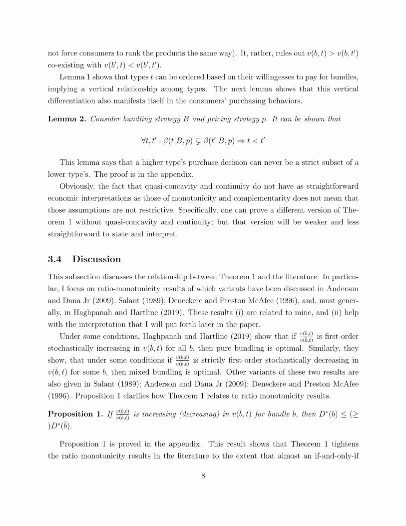
Example 1. Suppose n = 2, and t is uniformly distributed between 0 and 1. Assume

the firm can produce these products at no cost. By b denote the bundle {1}. For simplicity,

assume the complementary bundle bc = {2} is not valued by any type: ∀t : v({2}, t) = 0. A

common example of this is when {2} is an “add on,” which is not of value by itself but can

add value once the “base product” is present (e.g., additional memory for a smart phone).

Suppose ∀t : v(b, t) = t. For v(b, t), consider two cases.

Case 1: suppose ∀t : v(b, t) = t+ t2. That is, each type t’s valuation of the add on on top

of the original product is t2. It is straightforward to verify that v(b,t)

v(b,t)is strictly decreasing

in v(b, t). It is also straightforward to verify that D∗(b) = 0.5 and D∗(b) = 0.42 < 0.5.

Finally, one can show that the optimal strategy for the firm would be to offer b at the price

of 0.5 alongside b at the price of 0.94. In sum, the optimal strategy is in line with both what

Theorem 1 predicted and what ratio monotonicity would predict.

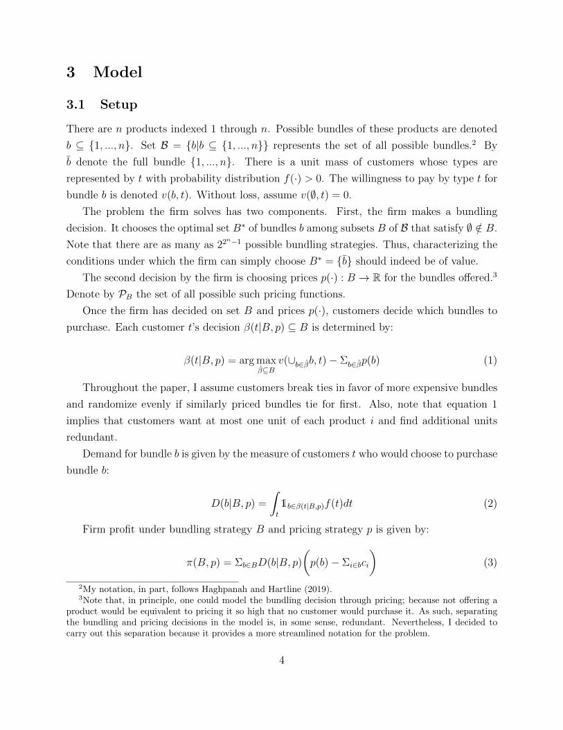
Case 2: suppose ∀t ≥ 0.3 : v(b, t) = t+ t2 and ∀t ≤ 0.3 : v(b, t) = t+√t× 0.32√

0.3. That is,

the “add on value” is initially concave in t and then becomes convex like Case 1 (see Figure

1a for a comparison between valuations in Case 1 v.s. that in Case 2). In this case, v(b,t)

v(b,t)

becomes strictly increasing in v(b, t) over t ∈ (0, .3), which does not satisfy the necessary

conditions in Haghpanah and Hartline (2019). Nevertheless, we still have D∗(b) = 0.5 and

D∗(b) = 0.42 < 0.5. One can also show that the optimal strategy by the firm is the same

unbundling strategy that we arrived at in Case 1.

Example 2. With the exception of v(b, t) assume the exact same setup as in Example

1. For v(b, t) consider two cases:

Case 1. suppose ∀t : v(b, t) = t+√t. That is, each type t’s valuation of the add on on top

of the original product is√t. It is straightforward to verify that v(b,t)

v(b,t)is strictly increasing in

v(b, t). It is also straightforward to verify that D∗(b) = 0.5 and D∗(b) = 0.59 > 0.5. Finally,

one can show that the optimal strategy for the firm would be to only offer b at the price of

1.05. In sum, the optimal strategy is in line with both what Theorem 1 predicted and with

ratio monotonicity.

Case 2: suppose ∀t ≥ 0.3 : v(b, t) = t +√t and ∀t ≤ 0.3 : v(b, t) = t + t2 ×

√0.3

0.32. That

is, the “add on value” is initially convex in t and then becomes concave like Case 1 (see

Figure 1b for a comparison between valuations in Case 1 v.s. that in Case 2). In this case,

9

0.0

0.5

1.0

1.5

2.0

0.00 0.25 0.50 0.75 1.00t

v

bundle

partial

full (case 1)

full (case 2)

(a) Example 1

0.0

0.5

1.0

1.5

2.0

0.00 0.25 0.50 0.75 1.00t

v

bundle

partial

full (case 1)

full (case 2)

(b) Example 2

Figure 1: Value functions in Examples 1 and 2

v(b,t)

v(b,t)becomes strictly decreasing in v(b, t) over the interval (0, 0.3). This does not satisfy

the necessary conditions in Haghpanah and Hartline (2019). Nevertheless, we still have

D∗(b) = 0.5 and D∗(b) = 0.59 > 0.5. One can also show that the optimal strategy by the

firm is the same pure bundling strategy that we arrived at in Case 1.

The examples constructed here modified valuations of those who did not purchase the

products. One can formulate other examples in which valuations of those who do purchase

get modified but we arrive at similar conclusions.

In addition to relating the results of this paper to the bundling literature, the examples

above should also highlight the simple implications these results have for price discrimination

decisions based on quality: price discrimination is optimal if the low quality version, if priced

optimally, sells more than the high quality version. A perhaps unsurprising consequence is

that price discrimination is more likely optimal when the higher quality version is more

costly to make (because higher marginal costs bring the optimal sales volume down.) This

also applies to the case of “damaged goods” Deneckere and Preston McAfee (1996): damage

the product if it helps sell more.

It is worth noting that in spite of providing (an almost) full characterization for pure

bundling, the results in this paper are not a strengthening of the previous literature. This

is because the background assumptions for Theorem 1 (i.e., assumptions 1 through 5) are

different from those in the literature. In particular, my assumptions are stronger than those

imposed in Haghpanah and Hartline (2019). As such, I view Theorem 1 as complementary

to (rather than a substitute for) the related results in the literature.

10

4 Interpretation of the result: complementarity, its

variation, and its co-variation with price sensitivity

Although the characterization of optimal bundling in Theorem 1 is intuitive, it is still worth

further discussing how this can be interpreted in terms of the primitives of the model (i.e.,

valuation function v). This section interprets Theorem 1 based on (i) how much variation

there is across consumers in the complementarity levels they see among products, and (ii)

how this variation is correlated with variation in price sensitivity.

Variation in complementarity levels: The condition ∀b : D∗(b) ≤ D∗(b) for optimal

pure bundling means that for all b we have D∗(b) ≤ D∗(bC |b) where bC = b \ b (this latter

inequality is implied by the quasi-concavity assumption. See proof of Theorem 1 in the

appendix.) That is, how many units bC would sell conditional on everyone having b plays

a crucial role. One determinant of D∗(bC |b) would be the variation among customers in

how much they value bC conditional on having b. If v(bC , t|b) is fairly homogeneous across t

(and if it is above Σi∈bCci), then the firm would optimally sell bC to the majority (or all) of

customers, likely surpassing D∗(b). If there is a large variation in v(bC , t|b), however, then the

chance of D∗(bC |b) < D∗(b) (and hence that of D∗(b|b) < D∗(b)) increases. As a result, the

analysis in this paper suggests that the variation across customers in the complementarity

level among products would be an important factor for optimal bundling decisions.

Correlation between complementarity and price sensitivity: The condition ∀b :

D∗(b) < D∗(b) for optimal pure bundling means that the demand level at which the price

elasticity for b hits -1 is higher than the that for other bundles.6 (note that this intuition

bears some resemblance to elasticity-based results from Long (1984); Armstrong (2013)). In

particular, for any bundle b, the aforementioned comparison holds both between b and b and

between bC = b \ b and b. That is, if we go through types in a descending way based on

v(b, t), then the willingness to pay for b dwindles less rapidly than does that for b or bC . In

other words, more price sensitive types must see a higher degree of complementarity between

b and bC than do less price sensitive types.

The aforementioned interpretation is also in line with the ratio monotonicity conditions

from Haghpanah and Hartline (2019); Anderson and Dana Jr (2009); Salant (1989); De-

neckere and Preston McAfee (1996) and has been mentioned by Haghpanah and Hartline

(2019). Suppose v(b, t) ≤ v(b, t′) for some t and t′. The sufficient ratio monotonicity con-

dition for optimality of pure bundling says v(b,t)

v(b,t)≤ v(b,t′)

v(b,t′)and v(bC ,t)

v(b,t)≤ v(bC ,t′)

v(b,t′). From these

6Though it is not necessary, to ease the interpretation assume all ci are zero.

11

inequalities, one can conclude

v(b, t)

v(b, t) + v(bC , t)≥ v(b, t′)

v(b, t′) + v(bC , t′).

This inequality, roughly, shows that the synergy between b and bC is from the perspective of

type t is higher than that for t′.

Based on this discussion, I propose that two key factors in optimal bundling decisions

are (i) how much variation there is across customers in the complementarity they see among

products, and (ii) how much this variation correlates with customers’ price sensitivity levels.

Next section verifies this interpretation using an empirical model of demand a la BLP.

5 Relevance of the interpretation of Theorem 1

This section tests the relevance and usefulness of the interpretation proposed in section

4 for applied work. Neither Theorem 1 in this paper nor, to my knowledge, any other

theoretical result in the literature provides a characterization that could be directly applied

to common econometric models of demand. Nevertheless, the informal interpretations that

I obtain in section 4 may potentially be useful. In this section, I examine the usefulness of

those interpretations for choosing the right model specification. I do this using a random

coefficient discrete choice model a la Berry et al. (1995).

Setup. To keep things simple, I again focus on a setting with two products where one

is the base product and the other an add on. Given that the add-on in and of itself is not

valuable by customers, I use the notation i ∈ {1, 2} for the basic and premium versions of

the product; i = 1 represents the basic version and i = 2 represents the version with the add

on.

Each customer t has a utility uit for product i. This utility is given by:

uit = α0 + α1,tpi + α2,t1i=2 + εit (5)

where α0 is a constant, α1,t is the price coefficient, α2,t is the valuation of the add-on, and

εit is the error term which has an Extreme Type I distribution. Note that both α1,t and α2,t

are heterogeneous across customers t. I assume that for each customer t, the pair (α1,t, α2,t)

is an independent draw from a bi-variate normal distribution:

12

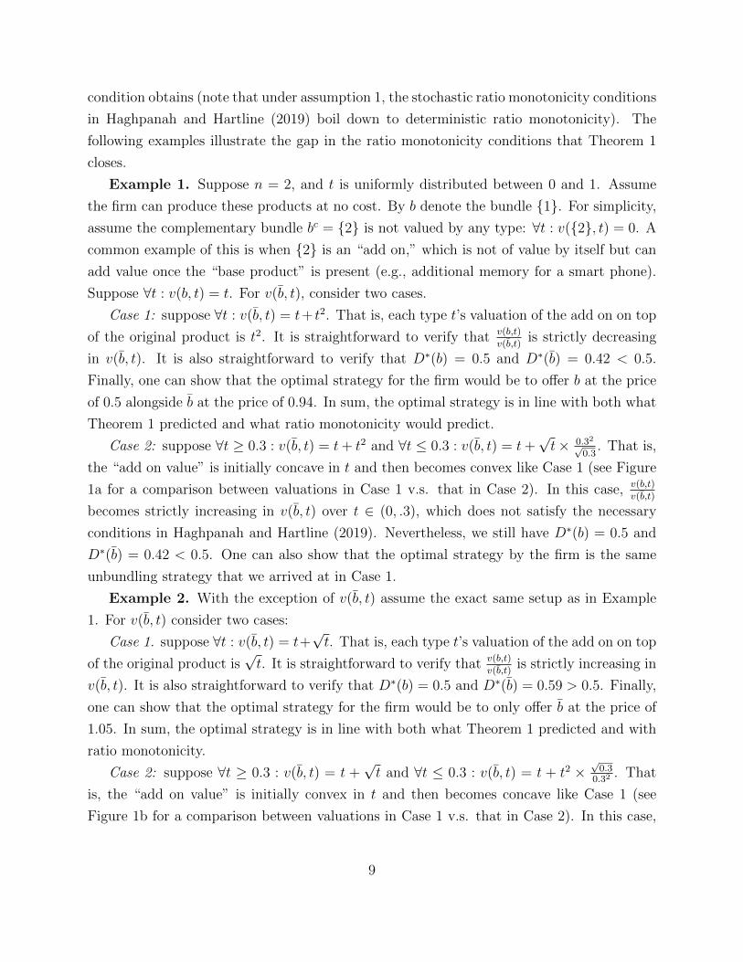
(α1,t, α2,t) ∼(

(µ1, µ2),

[σ2

1 σ1σ2ρ

σ1σ2ρ σ22

])(6)

where µ1 and µ2 are the means, σ1 and σ2 are the standard deviations, and ρ is the

correlation between the two coefficients.

Results. The question I study in this section is: when is it optimal for the firm to

offer both products i = 1 and i = 2 to the market, and when is it optimal to offer only

i = 2? Unfortunately, Theorem 1 does not directly apply to a market where the customers’

preferences are given by uit. Nevertheless, the interpretation proposed in section 4 may be

useful.

According to the interpretation provided in Section 4, there are two important objects

when it comes to bundling decisions: (i) the variation across customers t the complementar-

ity between products, and (ii) the correlation across customers between the complementarity

level and the price sensitivity. In our BLP setting, these two concepts translates to param-

eters σ2 and ρ respectively.

Based on our theoretical results, we expect pure bundling to be optimal when:

• σ2 is small, which means that the valuations for the add-on are so homogeneous that

it makes sense to give the add on to all purchasing customers.

• ρ is small (negative), which means more price sensitive customers (i.e., those with

smaller, more negative α1,t) will consider the add on to deliver a higher relative value

on top of the basic product.

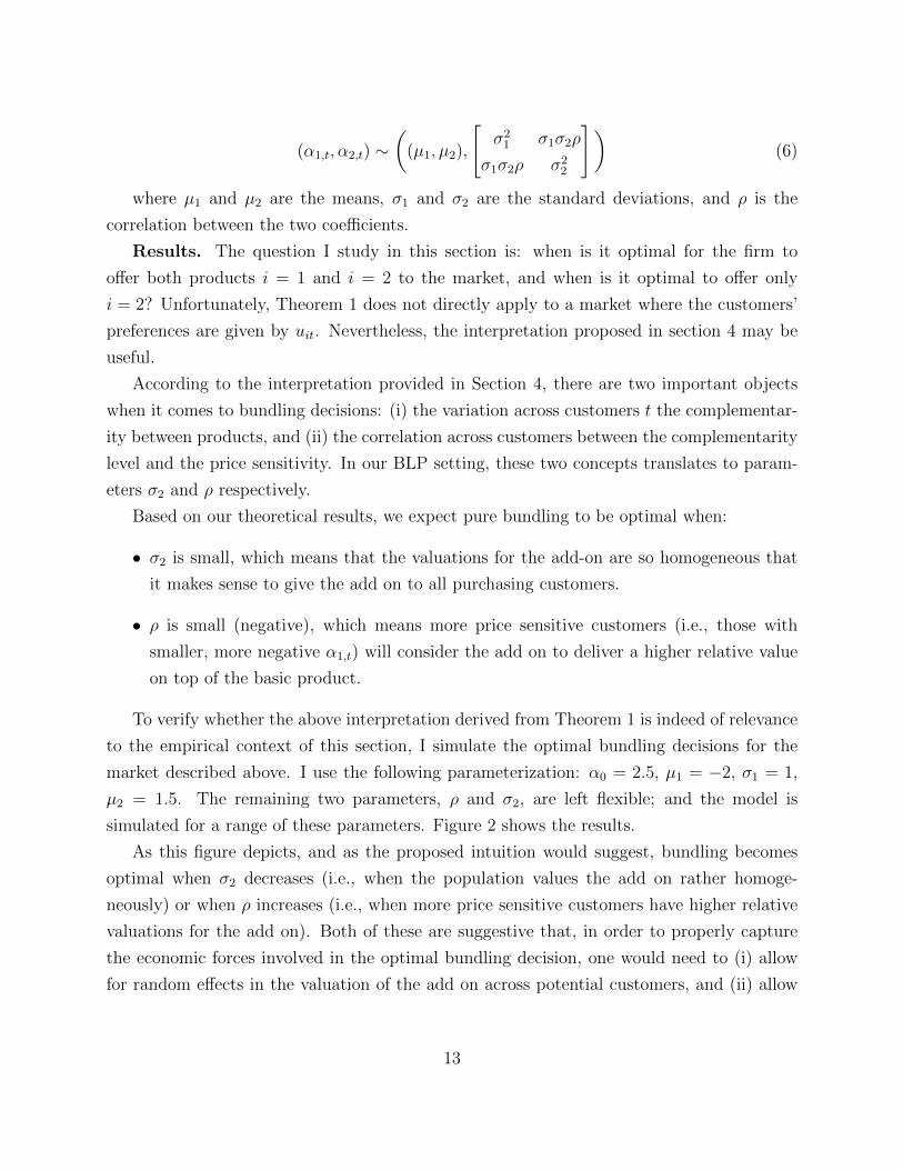
To verify whether the above interpretation derived from Theorem 1 is indeed of relevance

to the empirical context of this section, I simulate the optimal bundling decisions for the

market described above. I use the following parameterization: α0 = 2.5, µ1 = −2, σ1 = 1,

µ2 = 1.5. The remaining two parameters, ρ and σ2, are left flexible; and the model is

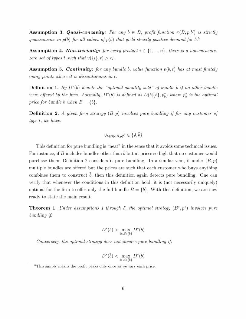
simulated for a range of these parameters. Figure 2 shows the results.

As this figure depicts, and as the proposed intuition would suggest, bundling becomes

optimal when σ2 decreases (i.e., when the population values the add on rather homoge-

neously) or when ρ increases (i.e., when more price sensitive customers have higher relative

valuations for the add on). Both of these are suggestive that, in order to properly capture

the economic forces involved in the optimal bundling decision, one would need to (i) allow

for random effects in the valuation of the add on across potential customers, and (ii) allow

13

0.00

0.25

0.50

0.75

1.00

−1.0 −0.5 0.0 0.5 1.0ρ

σ 2µ 2

Optimal_Strategy

Bundling

Unbundling

Figure 2: Optimal bundling decision as a function of parameters ρ and σ2 when otherparameters are fixed at α0 = 2.5, µ1 = −2, σ1 = 1, µ2 = 1.5. As expected, bundlingbecomes optimal when σ2 decreases (i.e., when the population values the add on ratherhomogeneously) or when ρ increases (i.e., when more price sensitive customers have higherrelative valuations for the add on).

for correlation between the random effects for add-on value and price sensitivity. I close this

section by making two concluding points.

First, as mentioned before, this simulation analysis does not prove that the observed

direction in the relationship between the optimal bundling decision and ρ or σ2. Though I

have not been able to find parameters that would reverse the direction, its possibility is not

ruled out.

The second point pertains to the relative importance of σ2 versus ρ in optimal bundling

decisions. Figure 2 suggests that there is a sense in which σ2 is more important than ρ. To

see this, note that there are values for σ2 under which the optimal decision is bundling (or

unbundling) regardless of what value ρ takes. The converse is not true, however; for any ρ, a

large enough σ2 implies unbundling is optimal and a small enough σ2 will make bundling the

optimal decision. The observation that a small (large) enough σ2 can always make bundling

(unbundling) optimal has been confirmed under all other parameterizations of the model

that I have examined. This latter point should, in my view, be considered good news for

the empirical analysis of bundling decisions; because it implies that if empirically identifying

the co-variation between α2,t and αi,t is not possible, then only capturing and identifying the

variation in α2,t may provide a reasonable approximation of the optimal bundling decision.

14

6 Conclusion And Future Research

In this paper, I completed two tasks. First, under a set of assumptions, I provided (an almost)

full characterization for the optimality of pure bundling.7 I showed that pure bundling is

optimal if the optimal quantity sold for the pure bundle (if sold alone) is strictly larger than

that for any sub-bundle. Conversely, pure bundling is sub-optimal if there is at least one

smaller bundle whose optimal sales volume (if sold alone) strictly surpasses that of the full

bundle.

Second, I used the characterization to arrive at an informal interpretation for when

bundling is optimal. I argued that to know whether to unbundle products, a firm would

need to know (i) the variability –across potential customers– in the complementarity level

among the products offered, and (ii) how much this variability correlates with variability

in price sensitivity. Finally, I showed the relevance of these interpretations to applied work

using a simulation of a random-coefficient discrete choice demand models.

The work in this paper can be extended in multiple directions. First, it would be valu-

able to investigate alternative assumptions to 1 through 5. In particular, it would be worth

studying whether the main takeaways of this paper would hold under alternatives to mono-

tonicity and complementarity. For instance, will bundling be so closely tied to sales volumes

if products were substitutes instead of complements? If not, would there be any other no-

tion that would fully characterize optimal bundling of substitute-able products in the same

way that sales volumes do for complementary ones? Similar questions apply to the role of

monotonicity: if instead of vertical differentiation, we had horizontal differentiation among

consumers, would there be a criterion that, under some conditions, fully characterize optimal

bundling in the same way that sales volumes do for vertically differentiated consumers?

Another useful direction for future research is one that–to the best of my knowledge–has

received little or no attention in the literature in spite of its importance: characterizing nec-

essary and sufficient conditions for bundling decisions in the context of widely used empirical

models. Ideally, such work would shed light on how to choose the right model specification

for studying bundling. To illustrate, the sales volume result in this paper, even if developed

using an empirical model, would not be directly useful (same is true of ratio monotonicity

results in Haghpanah and Hartline (2019); Anderson and Dana Jr (2009); Salant (1989); De-

neckere and Preston McAfee (1996) and elasticity results in Long (1984); Armstrong (2013)).

This is because, in order to directly evaluate the sales volume conditions, the econometrician

7As mentioned before, by replacing strict quasi-concavity of profits with strict concavity, we can bridgethe small gap in the characterization and obtain if-and-only-if.

15

needs an already-estimated model. But in that case, s/he can directly use the estimated

model to obtain the optimal bundling decision. Therefore, a useful theoretical result should

guide the empirical research process before, rather than after, the econometrician chooses

the empirical specification. I expect this task to be difficult. This is because commonly used

econometric models are set up to facilitate estimation rather than facilitate derivation of

theoretical results on matters such as optimal bundling. Thus, absent such direct results on

empirical models, using the “next best approach” taken by this paper may prove fruitful:

(i) obtain full characterization for pure/mixed bundling decisions using a different model;

(ii) obtain an economic interpretation for the developed theoretical result(s); (iii) verify the

relevance and insightfulness of the interpretation by simulating on the applied model of

interest.

References

William James Adams and Janet L Yellen. 1976. Commodity bundling and the burden of

monopoly. The quarterly journal of economics (1976), 475–498.

Eric T Anderson and James D Dana Jr. 2009. When is price discrimination profitable?

Management Science 55, 6 (2009), 980–989.

Mark Armstrong. 2013. A more general theory of commodity bundling. Journal of Economic

Theory 148, 2 (2013), 448–472.

Mark Armstrong. 2016. Nonlinear pricing. Annual Review of Economics 8 (2016), 583–614.

Steven Berry, James Levinsohn, and Ariel Pakes. 1995. Automobile prices in market equi-

librium. Econometrica: Journal of the Econometric Society (1995), 841–890.

Raymond J Deneckere and R Preston McAfee. 1996. Damaged goods. Journal of Economics

& Management Strategy 5, 2 (1996), 149–174.

Hanming Fang and Peter Norman. 2006. To bundle or not to bundle. The RAND Journal

of Economics 37, 4 (2006), 946–963.

Nima Haghpanah and Jason Hartline. 2019. When Is Pure Bundling Optimal? Penn State

University and Northwestern University (2019).

16

John B Long. 1984. Comments on” Gaussian Demand and Commodity Bundling”. The

Journal of Business 57, 1 (1984), S235–S246.

R Preston McAfee, John McMillan, and Michael D Whinston. 1989. Multiproduct monopoly,

commodity bundling, and correlation of values. The Quarterly Journal of Economics 104,

2 (1989), 371–383.

Domenico Menicucci, Sjaak Hurkens, and Doh-Shin Jeon. 2015. On the optimality of pure

bundling for a monopolist. Journal of Mathematical Economics 60 (2015), 33–42.

Gregory Pavlov. 2011. Optimal mechanism for selling two goods. The BE Journal of Theo-

retical Economics 11, 1 (2011).

Stephen W Salant. 1989. When is inducing self-selection suboptimal for a monopolist? The

Quarterly Journal of Economics 104, 2 (1989), 391–397.

Richard Schmalensee. 1984. Gaussian demand and commodity bundling. Journal of business

(1984), S211–S230.

George J Stigler. 1963. United States v. Loew’s Inc.: A note on block-booking. The Supreme

Court Review 1963 (1963), 152–157.

Jidong Zhou. 2017. Competitive bundling. Econometrica 85, 1 (2017), 145–172.

Jidong Zhou. 2019. Mixed Bundling in Oligopoly Markets. (2019).

A Proof of Theorem 1

I start by some preliminary remarks, definitions, and lemmas.

Remark 1. Suppose functions f1(x), f2(x) and f1(x) + f2(x) are all strictly quasi-concave

over the interval [a, b]. Then either (i) arg max f1 ≤ arg max f2 or (ii) arg max f1 ≤ arg max(f1+

f2) will imply:

arg max f1 ≤ arg max(f1 + f2) ≤ arg max f2.

The proof of this remark is left to the reader.

17

Definition 3. For disjoint bundles b and b′, denote by D∗(b|b′) the “optimal quantity sold”

of bundle b if all customers are already endowed with b′ but no other bundle is offered by the

firm. Formally, D∗(b|b′) is defined as D(b|{b}, p∗b|b′ , b′) where p∗b|b′ : {b} → R is effectively

one real number, and it is chosen among other possible p so that π({b}, p|b′) is maximized.

Next, I show that the problem of finding the optimal price for a bundle is equivalent to

the problem of finding the right type t∗ and sell to types t ≥ t∗.

Definition 4. Define by t∗(b|b′) the largest t such that 1 − F (t) ≥ D∗(b|b′). Also, for

simplicity, denote t∗(b|∅) by t∗(b).

Lemma 3. Consider disjoint bundles b and b′. Suppose that all types are endowed with

bundle b′, and that the firm is selling only bundle b, optimally choosing p∗b|b′. The set of types

who will buy the product at this price is the interval [t∗(b|b′), 1].

Proof of Lemma 3. Follows directly from monotonicity. Monotonicity implies that the

optimal sales volume D∗(b|b′) would be purchased by the highest types t with t weakly above

some cutoff t. Definition 4 says that for the demand volume to equal D∗(b|b′), the cutoff t

has to equal t∗(b|b′). Q.E.D.

Lemma 3 is important in that it shows the problem of choosing p∗b|b′ can equivalently be

thought of as the problem of choosing t∗b|b′ . This allows us to set up the firm’s problem based

on t. Next definition introduces a necessary notation for this purpose.

Definition 5. Consider disjoint bundles b and b′. Suppose that all potential customers have

already been endowed with b′, and that the firm is to sell only bundle b. By πb(t|b′) denote

the profit to the firm if it chose a price for bundle b such that all types t′ ≥ t would purchase

bundle b. More formally:

πb(t|b′) = π({b}, v(b, t|b′)|b′)

Lemma 4. πb(t|b′) is strictly quasi-concave in t.

Proof of Lemma 4. Suppose πb(t|b′) is not quasi-concave in t. This means there are

t1 < t2 < t3 such that πb(t2|b′) ≤ min(πb(t1|b′), πb(t3|b′)). Then construct p1, p2 and p3 from

t1, t2 and t3 according to the procedure in definition 5. That is, set pi = v(b, t|b′) for each i.

Monotonicity puts p2 strictly between p1 and p3. Note that for these prices, we have:

π({b}, p2|b′) ≤ min(π({b}, p1|b′), π({b}, p3|b′))

18

which violates the quasi-concavity assumption in p. Q.E.D.

With the above definitions and lemmas in hand, we are ready to prove the main theorem.

I start by the necessity condition (i.e., the condition that D∗(b) ≥ D∗(b) for all b is necessary

for pure bundling to optimal).

Proof of necessity. We want to show that if there is some b such that D∗(b) > D∗(b),

then pure bundling is sub-optimal. Specifically, I show that offering bundles b and bC = b \ bwould be strictly more profitable to the firm compared to offering b alone. The argument

follows.

Lemma 5. D∗(b) > D∗(b) implies D∗(b) > D∗(bC |b).

Proof of Lemma 5. Suppose, on the contrary, that D∗(b) ≤ D∗(bC |b). This means

t∗(b) ≥ t∗(bC |b). We know:

t∗(b) = arg maxtπb(t)

and

t∗(bC |b) = arg maxtπbC (t|b).

Also, given definition 4, it is straightforward to verify that:

πb(t) ≡ πbC (t|b) + πb(t)

By strict quasi-concavity of all profits in t and by remark 1, it has to be that the argmax

of πb(t) falls in between the argmax values t∗(bC |b) and t∗(b). Therefore, we get: t∗(b) ≤ t∗(b),

which implies D∗(b) ≤ D∗(b), contradicting a premise of the lemma. Q.E.D.

Lemma 6. Selling D∗(bC |b) units of bundle bC along with D∗(b) units of bundle b would be

strictly more profitable to the firm compared to selling D∗(b) units of the full bundle alone.

Proof of Lemma 6. In order to complete this proof, I first introduce a modified problem

for the firm.

Modified Firm Problem: Suppose the firm is to choose the optimal set B∗ of bundles and

optimal prices p∗ under the following conditions:

• The set B∗ can only be constructed from members of {∅, b, bC , b}.

• The valuation function is v rather than v. The function v over the set {∅, b, bC , b} is

defined by:

19

∀t :

v(∅, t) = v(∅, t) = 0,

v(b, t) = v(b, t)

v(bC , t) = v(bC , t|b)

v(b, t) = v(b, t) = v(b, t) + v(bC , t)

The only bundle for which v deviates from v is bC . By this construction, there is no

complementarity or substitution between b and bC under v. Also note that v is always

greater than or equal to v. Finally note that v inherits monotonicity and quasi-concavity.

Denote the profit and demand functions under the modified problem by π(·) and D(·)respectively.

The rest of the proof of the necessity conditions of Theorem 1 is organized as follows.

I first make a series of claims (without proving them) about the optimal solution to the

modified problem and its relationship with the optimal solution to the original problem.

Then I use these claims to prove the necessity conditions of the theorem. Finally, I go back

providing the proofs to these claims.

Claim 1. Consider the modified problem. Denote B1 = {b, bC}. Also denote by p1,∗ the

optimal pricing strategy given B1 under the modified problem. Similarly, construct B2 = {b}and p2,∗. Then, the following is true:

π(B1, p1,∗) > π(B2, p2,∗)

Claim 2. Consider the original problem (i.e., under value function v). Construct the set

B1 = {b, bC}, the same way as in the previous claim. Also denote by p1,∗ the optimal pricing

strategy given B1 under the original problem. Then one can show that p1,∗ = p1,∗ and:

π(B1, p1,∗) = π(B1, p1,∗)

Claim 3. Consider the original problem (i.e., under value function v). Set B2 = {b}, the

same way as in claim 1. Also denote by p2,∗ the optimal pricing strategy given B2 under the

original problem. Then one can show that p2,∗ = p2,∗ and:

π(B2, p2,∗) = π(B2, p2,∗)

Together, claims 1 through 3 yield:

20

π(B2, p2,∗) < π(B1, p1,∗)

This completes the proof of the necessity conditions of the theorem, provided that claims

1 through 3 are correct. That is, it is optimal for the firm to offer B1, p∗,1, which will lead

types t∗(bC |b) and above to buy both of the bundles and form b, and types in the interval

[t∗(b), t∗(bC |b)) to buy only b.

Next, I show claims 1 through 3 indeed hold.

Proof of Claim 1. Recall that under valuations v, the two products are independent

of each other. Therefore, for bundling strategy B1, the firm will choose the optimal prices

for b and bC separately. This will lead to selling D∗(bC |b) units of bC and D∗(b) units of b

under optimal pricing.8

Also recall that under v(b, t) = v(b, t) for all t. Therefore, under the modified problem

and under B2, the optimal price p2,∗ will be one that leads to exactly D∗(b) units sold.

Note that given monotonicity and the independence feature of v, the firm could replicate

using B1 any strategy that it can implement with B2. In particular, the firm could replicate

the profit from (B2, p2,∗) using B1 by setting prices p(b) and p(bC) such that each product sells

exactly D∗(b) unit of b and D∗(b) units of bC . This will yield exactly the profit of π(B2, p2,∗).

But we know at least one of these quantities sold is sub-optimal. This is because, by lemma

5, we have D∗(bC |b) < D∗(b). Therefore, by selling D∗(b) units for b and bC , at least one of

the quantities will be strictly sub-optimal.. This finishes the proof of this claim. Q.E.D.

Proof of Claim 2. To see why this claim is true, consider bundling strategy B1 under

the original problem. Assume the firm sets p1,∗ to be equal to p1,∗. It is straightforward to

verify that the demand volumes for b and bC in these conditions will be exactly equal to

those under the modified problem when the firm strategy is (B1, p1,∗). Therefore, the firm

can achieve π(B1, p1,∗) under the original problem.

Next, I show that the firm cannot achieve more than π(B1, p1,∗) under the original prob-

lem by choosing other values for p(b) and p(bC). To see this, consider two cases regarding

the firm’s pricing strategy:

Case 1. If the firm sets p(b) and p(bC) in a way that D(b) ≥ D(bC), the firm will get

the exact same demand volumes for the two bundles under the original problem as it would

8Note that independent values of b and bC under v would not generally imply that the firm wouldoptimally unbundle and set the optimal prices for b and bC separately. An clear example of when the firmstrictly prefers pure bundling over selling b and bC separately is Adams and Yellen (1976). Nevertheless,under monotonicity, one can indeed show that independence of values leads to optimality of unbundling andindependence of optimal prices from each other. The proof of this is straightforward and left to the reader.

21

under the modified one. Hence, the firm will also get the exact same profits under the two

problems with such prices: π(B1, p) = π(B1, p).

Case 2. If, however, the firm sets p(b) and p(bC) such that D(b) < D(bC), then by the

construction of v from v and by the complementarity property of v, we have D(bC) ≤ D(bC).

This, in turn, due to complementarity, will lead to D(b) ≤ D(b). Under these conditions, any

pricing strategy such that p(b) ≥ Σi∈bci and p(bC) ≥ Σi∈bCci will lead to π(B1, p) ≤ π(B1, p).

Therefore, for all pricing strategies with non-negative profit (which include all the candi-

dates for p1,∗) we have π(B1, p) ≤ π(B1, p). This, combined with the fact that p1,∗ delivers

the exact same profit under v as it does under v (where it is the unique optimum,) implies

that p1,∗ also uniquely maximizes π(B1, p) over different possible p. Q.E.D.

Proof of Claim 3. Note that v(b, t) = v(b, t) for all t. Therefore, optimizing the price

of b under v and v is identical, implying this claim. Q.E.D.

Given the proofs of the claims, the proof of the if side of the theorem is now complete.

Q.E.D.

Next, I turn to the proof of the sufficiency conditions (i.e., that D∗(b) > maxb∈B\{b}D∗(b)

implies that pure bundling is optimal).

Proof of sufficiency. I start with some lemmas.

Proof of Lemma 2 from the main text. Suppose, on the contrary, that β(t|B, p) (β(t′|B, p). for some t′ < t. That is:

β , β(t|B, p) \ β(t′|B, p) 6= ∅

I demonstrate that we can arrive at a contradiction by showing that type t′, when endowed

with β(t′, B, p), would have the incentive to buy β. Formally, I show:

v(β, t′|β(t′|B, p)) ≥ Σi∈βp(i) (7)

To see this, first note that by construction, type t, conditional on being endowed with

β(t′|B, p), would find it optimal to purchase β in order to obtain β(t|B, p). Formally:

v

(β, t|β(t′|B, p)

)≥ Σi∈βp(i) (8)

By monotonicity and t′ > t, we get:

v

(β, t′|β(t′|B, p)

)≥ v

(β, t|β(t′|B, p)

)(9)

22

Together, inequalities 8 and 9 imply inequality 7, completing the proof of the lemma.

Q.E.D.

Lemma 7. Under assumptions 1 through 4, and under firm optimal strategy (B∗, p∗), there

is a customer t such that β(t|B∗, p∗) = b.

Proof of Lemma 7. Assume, on the contrary that no type t purchases b under the

optimal firm behavior. I show we can reach a contradiction. In paricular, I show that type

t = 1 not purchasing b leads to a contradiction.

Assume ∪t∈[0,1]β(t|B∗, p∗) 6= b. That is, if we denote ∪t∈[0,1]β(t|B∗, p∗) by b, then bC 6= ∅.One can show that:

v(bc, 1) > Σi∈bCci (10)

To see why (10) is true, note that by complementarity:

v(bc, 1) ≥ Σi∈bCv({i}, 1) (11)

Also, by the fact that for each i there is some t with v({i}, t) > ci, and by monotonicity,

we have

Σi∈bCv({i}, 1) > Σi∈bCci (12)

Together, inequalities 11 and 12 imply inequality 10.

Given 10, and given that we are assuming no customer is buying any product within bC ,

the firm can (i) drop from B∗ any bundle that includes any element of bC , and (ii) then

introduce bC at the price of v(bC , 1). This move will lead at least type 1 to purchase the

bundle, which is profitable to the firm. Also, this move will not hurt the profit of the firm by

leading customers to not purchase bundles they bought before the introduction of bC . This

is because, for any type t, there are two cases. Case 1- type t will not buy newly introduced

bC : in this case her preferences over other bundles, and hence her purchase decisions on other

bundles remain unchanged. Case 2- type t does buy bC : in this case, by complementarity,

the valuations by t of all of the other product t has bought increases, which means t will still

buy those other products.

Therefore, we showed that if no type purchases b under (B∗, p∗), there will be a contra-

diction. This completes the proof of the lemma. Q.E.D.

In light of lemma 7, the following two corollaries of lemma 2 are useful.

23

Corollary 1. Under any (B, p), the set of types to for which β(t|B, p) = b takes the form

of [t1, 1] for some t1 < 1.

Corollary 2. Under any (B, p), the set of types to for which β(t|B, p) = ∅ takes the form

of [0, t2) for some t2 < 1.

With these lemmas in hand, I next turn to the proof of the sufficiency conditions. The

strategy is, again, contrapositive.

Assume on the contrary that we have, at the same time: (i) ∀b : D∗(b) ≤ D∗(b) and (ii)

the firm’s optimal strategy does not involve pure bundling. This latter statement implies

that the set of all distinct bundles chosen by customers under (B∗, t∗) includes members

other than ∅ or b. Formally, if we denote

β∗ = {b|∃t : β(t|B∗, p∗) = b}

then β∗ \ {∅, b} 6= ∅. In other words, our contrapositive assumption implies that t1 in

corollary 1 is stictly larger than t2 in corollary 2.

Then, note that by corollary 1 and the continuity assumption, there is some bundle

b1 ∈ β∗ \ {∅, b} such that for t′1 close enough to but smaller than t1, we have:

∀t ∈ [t′1, t1) : β(t|B∗, p∗) = b1 (13)

Also, by corollary 2 and the continuity assumption, there is some bundle b2 ∈ β∗ \ {∅, b}such that for t′2 close enough to but larger than t2, we have:

∀t ∈ [t2, t′2] : β(t|B∗, p∗) = b2 (14)

The rest of the proof of the sufficiency conditions of the theorem is organized as follows.

I first make a series of claims (without proving them). Next I use the claims to prove the

sufficiency conditions of the theorem. Finally, I will return to the proofs of the claims.

Claim 4. t∗(bC1 |b1) = t1.

In words, claim 4 says that the set of customers who purchase the full bundle β(t|B∗, p∗) =

b under the firm optimal strategy (B∗, p∗) is the same as those who purchase bC1 and construct

the full bundle if (i) everyone is endowed with b1 and (ii) the firm offers only bC1 , pricing it

optimally.

Claim 5. t∗(b2) = t2.

24

Claim 5 says that the set of customers who purchase b2 under the firm optimal strategy

(B∗, p∗) is the same as those who purchase b2 if the firm offers only b2 and prices it optimally.

Next, note that the assumption D∗(b) > D∗(b2), combined with monotonicity and claim

5, implies t∗(b) ≤ t2. By t1 > t2, we get t∗(b) < t1 = t∗(bC1 |b1). Also note that:

∀t : πb(t) = πbC1 (t|b1) + πb1(t)

As such, by strict quasi-concavity of profits, by t∗(b) < t∗(bC1 |b1), and by remark 1, the

peak of πb(t) should happen in between those of πbC1 (t|b1) and πb1(t). Therefore, we should

have: t∗(b1) ≤ t∗(b) ≤ t∗(bC1 |b1). But t∗(b1) ≤ t∗(b) implies:

D∗(b1) ≥ D∗(b)

which is a contradiction. Therefore, the sufficiency part of the theorem is true provided

that claims 4 and 5 are true. I now turn to the proofs of these claims.

Proof of Claim 4. Suppose on the contrary that t∗(bC1 |b1) 6= t1. In that case, it can be

shown that the firm can strictly improve its profit by slightly adjusting the price of bC1 . That

is, there is a pricing strategy p with p(b) = p∗(b) for all b 6= bC1 such that π(B∗, p) > π(B∗, p∗).

To see why this is the case, construct bundling strategy B′ in the following way:

B′ = {b1, bC1 } (15)

Also construct pricing strategy p′ by fixing p′(b1) = mint v(b1) but keeping p′(bC1 ) ad-

justable.

Now note that as long as ρ ∈ [p∗(bC1 )− ε, p∗(bC1 ) + ε] for a small enough ε, then π(B∗, p)

and π(B′, p′) move in parallel if we set p(bC1 ) = p′(bC1 ) = ρ and move ρ. The range parameter

ε should be chosen so that for any pricing strategy p constructed with a ρ in this interval we

have: D(bC1 |B∗, p) < 1 − F (t′1) where t′1 was constructed in equation 13. In other words, ε

should be small enough so that every type t in this interval purchases a (weak) super-set of

b1 under the optimal strategy.

Profits move in parallel because a small price change for bundle bC1 only changes the

purchase decisions of those types t who are sufficiently close to t1. All such customers have

decided to purchase b1 under (B∗, p∗). Therefore, under our constructed (B∗, p), these types’

valuations of bC1 will exactly be given by v(bC1 , t|b1)− p(bC1 ) which is exactly how these types

would value it under (B′, p′). Also, when some of these types drop bC1 in response to a

change in ρ, they will not drop any subset of b1 alongside it. This is because, even though

25

complementarities exist, these types t are all larger enough than t′1 so that by monotonicity

they value all components of b1 in B∗ above the collective price charged by p∗ for b1. To

sum up, a small enough change in ρ as part of pricing strategies p and p′ will lead to the

exact same reaction by customers and, hence, the exact same change in profits. Therefore,

the optimal value of ρ in this interval is the same under (B∗, p) as it is under B′, p′ (by strict

quasi-concavity, we know that this optimal ρ is unique in both cases). This common optimal

value for ρ leads to the exact same demand for bC1 under (B∗, p) as it does under (B′, p′).

The optimal demand under (B∗, p) is achieved by choosing ρ to equate p with p∗, which by

construction leads to all t with t ≥ t1 buying. The optimal ρ under (B′, p′), by definition,

should lead to all t ≥ t∗(bC1 |b1) buying. Therefore, if t1 6= t∗(bC1 |b1), then one can modify

(B∗, p∗) by slightly changing p∗(bC1 ) and improve the profit, a contradiction. Q.E.D.

Proof of Claim 5. The proof of this claim is fairly similar to that of the previous claim.

We start by assuming, on the contrary, that t∗(b2) 6= t2 and reach a contradiction. Construct

(B′, p′) by assuming B′ = {b2}, which makes p′ just one number (for the price of b2). Similar

to the previous claim, one can show that for prices ρ for b2 sufficiently close to p∗(b2) the two

profit functions π(B∗, p) and π(B′, p′) move in parallel as we move ρ. Again, similarly to the

previous claim, this implies that (B∗, p∗) can be improved upon if t2 6= t∗(b2). Q.E.D.

The completion of the proofs for claims 4 and 5 finishes the proof of the sufficiency side

of the theorem, and hence the theorem itself. Q.E.D.

B Proofs of Other Results

Proof of Proposition 1. I prove the statement outside of parentheses: If v(b,t)

v(b,t)is decreasing

in v(b, t) for bundle b, then D∗(b) ≤ D∗(b). The version inside parentheses can be proven in

a similar way.

Assume on the contrary that v(b,t)

v(b,t)is increasing but D∗(b) > D∗(b). Denote by π∗(b) the

amount of profit the firm obtains by selling only b and optimally pricing it, which yields the

demand level D∗(b). Given that production costs are assumed zero, we have:

π∗(b) = v(b, t∗(b))×D∗(b) (16)

Using a similar notation for b, we get:

π∗(b) = v(b, t∗(b))×D∗(b) (17)

26

By our assumption that D∗(b) > D∗(b), we get t∗(b) < t∗(b). Also, by π∗(b) and π∗(b)

being the profits from optimal decisions, and by quasi-concavity, we know that the firm’s

profit would be strictly lower than π∗(b) if it were to sell D∗(b) units of b instead of D∗(b)

units. Likewise, its profit would fall strictly below π∗(b) if it were to sell D∗(b) units of b

instead of D∗(b) units. Formally:

π∗(b) > v(b, t∗(b))×D∗(b) (18)

and:

π∗(b) > v(b, t∗(b))×D∗(b) (19)

Replacing from 16 and 18, and also 17 and 19, we get:

v(b, t∗(b))×D∗(b) > v(b, t∗(b))×D∗(b) (20)

and:

v(b, t∗(b))×D∗(b) > v(b, t∗(b))×D∗(b) (21)

Multiplying the left-hand-side terms of inequalities 20 by each other and doing the same

for the right-hand-side terms, then removing the terms that cancel out and rearranging, one

can obtain:

v(b, t∗(b))

v(b, t∗(b))>v(b, t∗(b))

v(b, t∗(b))(22)

But inequality 22, combined with t∗(b) < t∗(b) and monotonicity, violates the premise of

the proposition, a contradiction. Q.E.D.

27