BUILDING BLOCKS FOR SYSTEMS MODELS Quote of...

Lecture Notes for Ecological Modeling --- Jianguo (Jingle) Wu

BUILDING BLOCKS FOR SYSTEMS MODELS

Quote of the Day

“To do science is to search for repeated patterns, not simply to accumulate facts..." - Robert H. MacArthur (1972)

I. WHY BUILDING BLOCKS? Building blocks, or simulation modules are simple models that represent some basic system structures and dynamics. These modules are very important for understanding many fundamental processes common in biological, physical, and socioeconomic phenomena. One certainly needs to understand them well before attempting to deal with complex feedback systems. In the same time, the model building blocks demonstrate how these commonly occurring basic processes are represented in systems simulation, and often become convenient and effective for constructing complex systems models. II. BUILDING BLOCKS FOR SYSTEMS MODELS (I) FIRST-ORDER SYSTEMS

o First-order: One state variable (or 1 stock) o Linear: No non-linear combinations of the state

variable of any sort in the algebraic equation of rates. 1. Linear Change

o One state variable. o One rate variable. o The rate of change is a constant, not dependent on the state variable. Thus, there is no

feedback loop. (1) Linear Growth

o The rate of change is positive, and thus represented as an inflow.

o Examples: o Increase in water level in a

tank with a constant inflow of water into the tank.

o Plant biomass sometimes is found to increase linearly with certain soil nutrients.

Linear Growth in STELLA X

dX dt X(t) = X(t - dt) + (dX_dt) * dt INIT X = 0 INFLOWS: dX_dt = 2

11:40 PM 4/7/97

0.00 3.00 6.00 9.00 12.00

Time

1:

1:

1:

2:

2:

2:

0.00

15.00

30.00

1.00

2.00

3.00

1: X 2: dX dt

1

1

1

1

2 2 2 2

Graph 1 (Linear Growth)


(2) Linear Decline o The rate of change is negative, and thus

represented as an outflow. o Examples:

Decrease in the amount of materials left in a stock when the materials are taken out of the stock in the same amount per unit of time.

Decrease in crop yield with declining annual precipitation sometimes exhibits linear pattern.

(3) Linear Growth and Decline

o Combination of the linear growth and decline module. o One state variable. o Either two uniflows (one

inflow and one outflow) or one biflow (compare the structural diagrams below).

o The uniflow version gives more details, whereas the biflow version is more concise. The choice of the two forms is dependent on the degree of details is needed.

o Linear growth occurs when the total rate of change (inflow minus outflow) is positive, and linear decline does otherwise.

Linear Decline in STELLA X

dX dt X(t) = X(t - dt) + (- dX_dt) * dt INIT X = 40 OUTFLOWS: dX_dt = 2

12:07 AM 4/8/97

0.00 3.00 6.00 9.00 12.00

Time

1:

1:

1:

2:

2:

2:

15.00

30.00

45.00

1.00

2.00

3.00

1: X 2: dX dt

1

1

1

1

2 2 2 2

Graph 1 (Linear Growth)

Linear Growth and Decline in STELLA (1) Two-uniflow model: (2) One-biflow model:

X

dX dt outdX dt in

Y

dY dt X(t) = X(t - dt) + Y(t) = Y(t - dt) + (dX_dt_in- dX_dt_out) * dt (dY_dt) * dt INIT X = 0 INIT Y = 40 INFLOWS: INFLOWS: dX_dt_in = 2 dY_dt = -1 OUTFLOWS: dX_dt_out = 1


2. Exponential Growth and Decay (1) Exponential Growth

• Also known as compounding process • One state variable. • One rate variable. • One auxiliary variable. • The rate of change is equal to a constant

proportion of the state variable. • Because the rate variable depends on the state

variable itself, they form a positive feedback loop, in which the state variable and the rate of change reinforce each other, generating an accelerating, run-away behavior.

• The rate of change is always positive (i.e., the state variable increases monotonically), and is represented it as an inflow.

• Time Constant Tc: The reciprocal of the constant r in the exponential model, Tc = 1/r, with the dimension of units of time. o For exponential growth, Tc is the time required

for the state variable to become e (= 2.7183) times of its current value. This can be seen from the following simple manipulations:

N = N

0ert .

When t is equal to Tc, we have

NTc

= N0e

1

Tc

Tc

= N0e

In general, if t = nTc,

NnTc

= N0e

1

Tc

nTc

= N0en

o Note: For continuous

systems, the time step, ∆t, in simulation must be smaller than the smallest time constant in the model.

• Doubling Time Td: The time required for the state variable in the exponential model to

double in value.

Exponential Growth in STELLA N

dN dt

r N(t) = N(t - dt) + (dN_dt) * dt INIT N = 2 INFLOWS: dN_dt = r*N r = 0.1

11:26 AM 4/8/970.00 12.50 25.00 37.50 50.00

Time

1:

1 :

1 :

2 :

2 :

2 :

0.00

150.00

300.00

0.00

15.00

30.00

1: N 2: dN dt

1 11

1

2 22

2

Graph 1: Page 1 (Exponenti…


To calculate the doubling time, let N = 2N0 and let t = Td. Thus, from N = N0ert , we have:

2N

0= N

0erT

d

ln 2 = rTd

Td=

0.69

r or T

d= 0.69 T

c

o Therefore, the doubling time for exponential growth is a constant. It is conversely proportional to the rate of change, and is about 70% of the time constant. This is where “the rule of 70” in population demography comes from (i.e., population doubling time = 70 / percent natural growth rate).

• Exponential growth is a common type of dynamics that exists in all different disciplines. Any phenomena described by words such as “snowball effect”, “vicious circles”, “virtuous circles”, and “bandwagon effect” can be represented as a positive feedback loop structure.

• Examples: o Savings increase in a bank account due to

interest income o Population growth when resources are not

limiting. o Drug addiction. o Arms race (proliferation).

• Superexponential (or supraexponential) growth: o In many positive feedback

systems, doubling time decreases, rather than remain constant, as the state variable increases. This means that the rate of change is a nonlinear function of the state variable (see Figure). For example,

dN

dt= (rN)N = rN

2

o The dynamics generated by this nonlinear system, with a rate of change faster than a fixed proportion of the state variable, is called superexponential growth.

o The superexponential growth has the same feedback structure as

1:36 PM 4/8/97

0.00 5.00 10.00 15.00 20.00

Time

1:

1 :

1 :

2 :

2 :

2 :

2.00

51.00

100.001: Super N 2: N

1

1

22

2

2

Graph 1: Page 1 (Superexponen… N(t) = N(t - dt) + (dN_dt) * dt INIT N = 10 INFLOWS: dN_dt = r*N Super_N(t) = Super_N(t - dt) + (dN_dt_super) * dt INIT Super_N = 10 INFLOWS: dN_dt_super = (r_2/10)*Super_N^2 r = 0.1 r_2 = if (time<10) then 0.1 else 0


the exponential. (2) Exponential Declay • Also known as draining process • One state variable. • One rate variable. • The rate of change is equal to a constant

proportion of the state variable, but in contrast with exponential growth it is negative.

• The rate variable depends on the state variable itself, and form a feedback loop between them. Because an increase in the value of the state variable increases the rate of change, but an increase in the rate decreases the value of the state variable, the feedback is negative (or goal-seeking). • Time constant Tc: The reciprocal of the constant r in the exponential model, Tc = 1/r,

with the dimension of units of time. o For exponential decay, Tc is the time required for the state variable to become e -1 (=

0.368) times of its current value, or the time required for 63% of the contents in the stock to vanish. This is also called the relaxation time, which is sometimes used as a measure of the speed with which a system is absorbing disturbances.

o Mathematically, relaxation time can be derived as follows: N = N

0e-rt ,

For a time period from t=0 to t=Tc,

NTc= N

0e

-1

Tc

Tc

= e-1N

0= 0.368 N

0,

In general, when t = nTc, we have

NnTc

= N0e

-1

Tc

nTc

= e- n

N0= 0.368

n

N0

• Half-life Th: The time required for the state variable to reduce its current value by a half. It is an analog of the doubling time in exponential growth. It can be calculated as follows:

1

2N0= N

0e- rT

h ,

ln1

2= -rT

h, or ln 2 = rT

h, thus,

Th=

0.69

r or T

h= 0.69 T

c

o Therefore, the half-life time for exponential decay is a constant (about 70% of the time constant), independent of the value of the state variable.

Exponential Decay in STELLA N

dN dt

r N(t) = N(t - dt) + (- dN_dt) * dt INIT N = 100 OUTFLOWS: dN_dt = r*N r = 0.1

11:45 AM 4/10/97

0.00 12.50 25.00 37.50 50.00

Time

1:

1 :

1 :

2 :

2 :

2 :

0.00

50.00

100.00

0.00

5.00

10.00

1: N 2: dN dt

1

1

11

2

2

22

Graph 1: Page 1 (Exponentia…


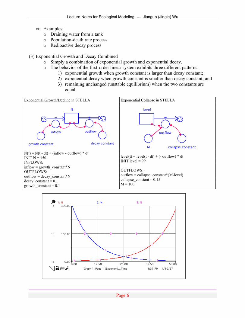
• Examples: o Draining water from a tank o Population-death rate process o Redioactive decay process

(3) Exponential Growth and Decay Combined

o Simply a combination of exponential growth and exponential decay. o The behavior of the first-order linear system exhibits three different patterns:

1) exponential growth when growth constant is larger than decay constant; 2) exponential decay when growth constant is smaller than decay constant; and 3) remaining unchanged (unstable equilibrium) when the two constants are

equal.

Exponential Growth/Decline in STELLA

N

outflow

decay constant

inflow

growth constant N(t) = N(t - dt) + (inflow - outflow) * dt INIT N = 150 INFLOWS: inflow = growth_constant*N OUTFLOWS: outflow = decay_constant*N decay_constant = 0.1 growth_constant = 0.1

Exponential Collapse in STELLA

level

outflow

collapse constantM level(t) = level(t - dt) + (- outflow) * dt INIT level = 99 OUTFLOWS: outflow = collapse_constant*(M-level) collapse_constant = 0.15 M = 100

1:37 PM 4/10/970.00 12.50 25.00 37.50 50.00

Time

1:

1 :

1 :

0.00

150.00

300.001: N 2: N 3: N

1 11

1

2

2

22

3 3 3 3

Graph 1: Page 1 (Exponenti…


3. Exponential Collapse • Also known as accelerated decay, indicating that the rate of change gets faster as the level

goes down. • A simple exponential collapse model may consist of 1 state variable, 1 outflow, and 2

constants. • A positive feedback: increasing level --> increasing rate of change --> increasing level --

> ... • A simple mathematical model for exponential collapse:

dN

dt= -r(M - N)

where N (< M) is the state variable, and r and M are two constants.

• Examples: o Population shrinking when smaller than MVP (minimum viable population). o Change in the interactive force between molecules when water is heated up and boils. o Decline of species diversity with increasing habitat fragmentation. o Some other threshold phenomena in physical and biological processes may exhibit

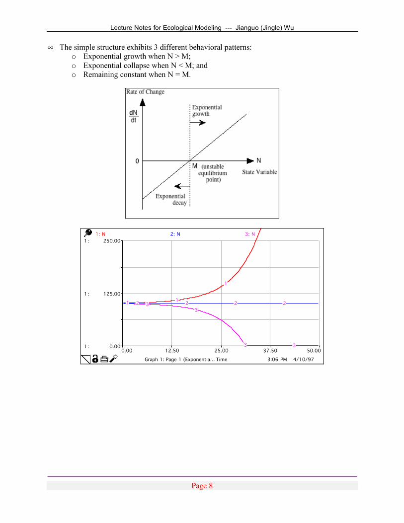
behavior that resembles exponential collapse. 4. Exponential Growth and Collapse Combined

• A simple exponential collapse consists of 1 state variable, 1 bi-directional flow, and two constants.

• This simple model can be mathematically expressed as: dN

dt= r(N - M)

Exponential Growth/Collapse in STELLA N

M

dN dt

r level(t) = level(t - dt) + (- outflow)*dt INIT level = 99 OUTFLOWS: outflow = collapse_constant*(M-level) collapse_constant = 0.15 M = 100


• The simple structure exhibits 3 different behavioral patterns: o Exponential growth when N > M; o Exponential collapse when N < M; and o Remaining constant when N = M.

3:06 PM 4/10/97

0.00 12.50 25.00 37.50 50.00

Time

1:

1 :

1 :

0.00

125.00

250.001: N 2: N 3: N

1 1

1

2 2 2 233

3 3

Graph 1: Page 1 (Exponentia…


5. Goal-Seeking Behavior (1) Simple Goal-Seeking

• A simple goal-seeking model may consist of 1 state variable, 1 biflow, and 2 constants.

• The state variable and the flow form a negative feedback.

• A simple goal-seeking model may take the form:

dL

dt= c(G - L)

where L is the level, G is the goal, and c is a constant. • Apparently, exponential decay is a special

case of goal-seeking behavior, in which the goal is zero!

(2) S-Shaped Growth

• Also known as logistic growth or sigmoidal growth.

• It is a first-order nonlinear system (see the Rate-Level graphs).

• The state variable and the flow form a negative feedback that ultimately gives rise to the goal seeking behavior (see the Forrester diagram).

• It may take different forms (uniflow or biflow versions). [For example, in population regulation, crowding may affect only the per capita birth rate, or only the per capita death rate, or both.]

Simple Goal-Seeking in STELLA

level

Inflow

goalconstant

discrepancy level(t) = level(t - dt) + (Inflow) * dt INIT level = 2 INFLOWS: Inflow = constant*discrepancy constant = 0.1 discrepancy = goal-level goal = 100

4:11 PM 4/10/97

0.00 12.50 25.00 37.50 50.00

Time

1:

1 :

1 :

0.00

100.00

200.001: level 2: level 3: level

1 1 1 1

2

22 2

3

33 3

Graph 1: Page 1 (Simple goa…

levelInflow

~

Rate Value level(t) = level(t - dt) + (Inflow) * dt INIT level = 300 INFLOWS: Inflow = Rate_Value Rate_Value = GRAPH(level)...

Rate-Level Graph


The behavior of this simple structure has three patterns: 1) Increasing and approaching the goal if simulation starts with a value of the level

smaller than the goal; 2) Decreasing and approaching the goal if simulation starts with a value of the level

larger than the goal; 3) Remaining unchanged if simulation starts with the value of the level equal to the goal.

5:08 PM 4/10/97

0.00 12.50 25.00 37.50 50.00

Time

1:

1 :

1 :

0.00

150.00

300.001: level 2: level 3: level

1

1

1

12 2 2 2

3

3 3 3

Graph 1: Page 1 (Simple sig… A familiar example of sigmoidal growth is the logistic equation:

dN

dt= rN(1 - N / K)

This is a first-order nonlinear differential equation. The following is an equivalent simple systems model.

N

dN dt

r

K

N(t) = N(t - dt) + (dN_dt) * dt INIT N = 2 INFLOWS: dN_dt = r*N*(K-N)/K K = 100 r = 0.2

10:46 PM 4/10/97N

0.00 50.00 100.000.00

2.50

5.00

1: N v. dN dt

Graph 1: Page 2 (Untitled Graph)

11:12 PM 4/10/97

0.00 12.50 25.00 37.50 50.00

Time

1:

1:

1:

0.00

100.00

200.00

1: N 2: N 3: N

1

1

1

1

2

2 2 23 3 3 3

Graph 1: Page 3 (Untitled Graph) 10:46 PM 4/10/97

0.00 12.50 25.00 37.50 50.00

Time

1:

1:

1:

2:

2:

2:

0.00

50.00

100.00

0.00

2.50

5.00

1: N 2: dN dt

1

1

1

1

2

2

2

2

Graph 1: Page 1 (Simple goal-seeking)

Dynamics from the Logistic Equation-Based Module


Feedback loop analysis of the S-shaped growth:

• Positive vs negative feedback regions • Characteristics of the rate-level curve: several similar, but distinctive forms • Goal-seeking does NOT always guarantee goal-achieving!


(II) SECOND-ORDER SYSTEMS First-order (continuous) systems do not generate overshoot and collapse or oscillations unless significant time delays are introduced. Such behavioral patterns are commonly found in second- or higher-order systems (with 2 or more stocks). The following section illustrates some simple systems structures that give rise to non-monotonic dynamics. 6. Overshoot and Collapse • A simple structure that generates

overshoot and collapse behavior includes 2 stocks (e.g., population and food resource) and a few rates associated with them (see the Forrester diagram).

• In this example, population grows exponentially when food is not limited. More and more food resource is consumed by the growing population, resulting in less and less food resource. At some point, death rate will rise above birth rate, and the population eventually collapse due to the lack of food.

Overshoot and Collapse in STELLA population

death ratebirth rate

per capita birth rate

food

~

per capita death rate

consumption rate

per capita consumption rate

food(t) = food(t - dt) + (- consumption_rate) * dt INIT food = 1000 {tones} OUTFLOWS: consumption_rate = per_capita_consumption_rate*population population(t) = population(t - dt) + (birth_rate - death_rate) * dt INIT population = 100 INFLOWS: birth_rate = per_capita_birth_rate*population OUTFLOWS: death_rate = per_capita_death_rate*population per_capita_birth_rate = 0.1 {1/time} per_capita_consumption_rate = 0.1 {tones/(individual * time)} per_capita_death_rate = GRAPH(food/INIT(food)) (0.00, 0.995), (0.1, 0.645), (0.2, 0.45), (0.3, 0.3), (0.4, 0.21), (0.5, 0.14), (0.6, 0.095), (0.7, 0.06), (0.8, 0.03), (0.9, 0.01), (1, 0.00)

12:13 AM 4/11/97

0.00 12.50 25.00 37.50 50.00

Time

1:

1 :

1 :

2 :

2 :

2 :

0.00

200.00

400.00

250.00

650.00

1050.00

1: population 2: food

1

1

1

1

2

2

22

Graph 1: Page 1 (Overshoot/c… 12:13 AM 4/11/97

0.00 12.50 25.00 37.50 50.00

Time

1:

1 :

1 :

2 :

2 :

2 :

3 :

3 :

3 :

0.00

20.00

40.00

0.00

30.00

60.00

0.00

0.20

0.40

1: consumption rate 2: death rate 3: per capita death rate

1

1

1

12

2

2

23

3

3

3

Graph 1: Page 2 (overshoot/c…


7. Oscillations • Two stocks and four

rates associated. • The first stock

promotes the inflow to the second stock, and the second stock accelerates the depletion of the first stock. This negative feedback is essential for oscillatory behavior.

• With STELLA, you must use one of the Runge-Kutta simulation algorithms.

(1) A Simple General Structure (cf. Richmond et al. 1993).

Oscillation in STELLA

inflow 2

Stock 1

inflow 1 outflow 1

productivity 1

outflow 2

Stock 2

productivity 2 Stock_1(t) = Stock_1(t - dt) + (inflow_1 - outflow_1) * dt INIT Stock_1 = 10 INFLOWS: inflow_1 = Stock_2*productivity_1 OUTFLOWS: outflow_1 = 10 Stock_2(t) = Stock_2(t - dt) + (inflow_2 - outflow_2) * dt INIT Stock_2 = 15 INFLOWS: inflow_2 = 10 OUTFLOWS: outflow_2 = Stock_1*productivity_2 productivity_1 = 1 productivity_2 = 1

2:21 AM 4/11/97

0.00 4.00 8.00 12.00 16.00

Time

1:

1 :

1 :

2 :

2 :

2 :

0.00

10.00

20.001: Stock 1 2: Stock 2

1

1

1

1

2 2

2

2

Graph 1 (Oscillation)


(2) A Predator-Prey Model

Oscillation in STELLA prey

prey births prey deaths

~

per capita birth rate

predator

birth rate death rate predator(t) = predator(t - dt) + (birth_rate - death_rate) * dt INIT predator = 10 INFLOWS: birth_rate = 0.01*predator*prey OUTFLOWS: death_rate = 0.2*predator prey(t) = prey(t - dt) + (prey_births - prey_deaths) * dt INIT prey = 50 INFLOWS: prey_births = per_capita_birth_rate*prey OUTFLOWS: prey_deaths = 0.03*predator*prey per_capita_birth_rate = GRAPH(prey) (0.00, 0.685), (50.0, 0.41), (100, 0.295), (150, 0.215), (200, 0.15), (250, 0.11), (300, 0.07), (350, 0.04), (400, 0.02), (450, 0.01), (500, 0.00)

2:25 AM 4/11/97

0.00 10.00 20.00 30.00 40.00

Time

1:

1:

1:

2:

2:

2:

5.00

30.00

55.00

10.00

25.00

40.00

1: prey 2: predator

1

1

1

1

2

2

2

2

Graph 1 (Untitled Graph) 2:47 AM 4/11/97

0.00 25.00 50.00 75.00 100.00

Time

1:

1:

1:

2:

2:

2:

0.00

45.00

90.00

0.00

25.00

50.00

1: prey 2: predator

1 1

1

1

2 22

2

Graph 1 (Untitled Graph) (From the same model but D-I prey birth rate)


(III) OSCILLATIONS GENERATED BY DRIVING FUNCTIONS o Driving variables (or functions) that change periodically (e.g., temperature, light intensity)

may introduce oscillations into a system of any order. o Oscillations forced by driving variables are called externally generated oscillations.

A general equation for modeling periodic driving functions: Y =m + Acos(w(t - t )) where Y is a driving variable (e.g., temperature, light intensity), m is the mean value of the function, A is the amplitude of the peak above the mean, (t - t ) shifts the peak by t physical units, and the w is the angular frequency per physical unit. For example, suppose we have a time series:

o Mean daily air temperatures: 40 degrees F o Amplitude: 25 degrees F o Period: 365 days o Position of the 1st peak: July 30 (Julian day 211)

The equation becomes:

T = 40 + 25cos2p365

( t - 211)Ê Ë

ˆ ¯

Externally Generated Oscillation

stock

inflow outflow

driving variable time in stoch stock(t) = stock(t - dt) + (inflow - outflow) * dt INIT stock = 5 INFLOWS: inflow = driving_variable OUTFLOWS: outflow = stock/time_in_stoch driving_variable = SINWAVE(4,20)+3 time_in_stoch = 1 {time unit}

8:50 AM 4/11/97

0.00 15.00 30.00 45.00 60.00

Time

1:

1 :

1 :

2 :

2 :

2 :

0.00

3.50

7.00

-1.00

3.00

7.00

1: stock 2: driving variable

1

1

1

12

2

2

2

Graph 1 (Oscillation by Driving…


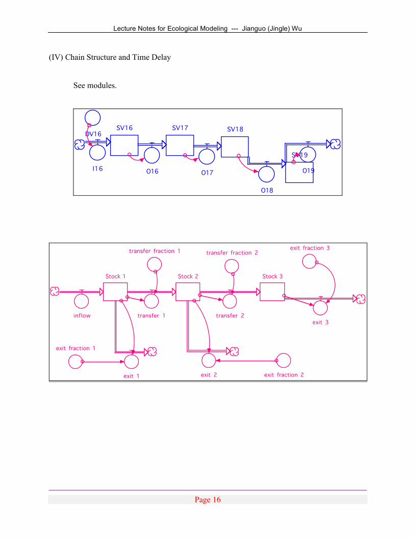
(IV) Chain Structure and Time Delay See modules.

SV16 SV17 SV18

SV19

I16O16 O17

O18

O19

DV16

Stock 1

inflow

Stock 2 Stock 3

transfer 1 transfer 2

exit 3

exit 2exit 1

transfer fraction 1 transfer fraction 2

exit fraction 1

exit fraction 2

exit fraction 3

BUILDING BLOCKS FOR SYSTEMS MODELS Quote of...

Documents

Transcript of BUILDING BLOCKS FOR SYSTEMS MODELS Quote of...