Generated using version 3.0 of the official AMS LATEX template

Testing the role of radiation in determining tropical cloud top1

temperature2

Bryce E. Harrop ∗ and Dennis L. Hartmann

Department of Atmospheric Sciences, University of Washington, Seattle, Washington

3

∗Corresponding author address: Bryce E. Harrop, Dept. of Atmospheric Sciences, University of Wash-

ington, Box 351640, Seattle, WA 98195-1640.

E-mail: bryce@atmos.washington.edu

1

ABSTRACT4

A cloud-resolving model is used to test the hypothesis that radiative cooling by water vapor5

emission is the primary control on the temperature of tropical anvil clouds. The temperature6

of ice clouds in the simulation can be increased or decreased by changing only the emissivity of7

water vapor in the upper troposphere. The effect of the model’s fixed ozone profile on stability8

creates a pressure-dependent inhibition of convection, leading to a small warming in cloud9

top temperature as SST is increased. Increasing stratospheric water vapor also warms the10

cloud top temperature slightly. Changing the latent heat of fusion reduces the cloud fraction11

at high altitudes, but does not significantly change temperature at which cloud fraction12

peaks in the upper troposphere. The relationship between radiatively-driven horizontal mass13

convergence and cloud fraction that causes cloud temperature to be insensitive to surface14

temperature is preserved when a large model domain is used so that convection aggregates15

in a small part of the model domain.16

1. Introduction17

Climate feedbacks involving water vapor and clouds are very important for the magni-18

tude and structure of climate change, and the strongest energy exchanges are in the Tropics.19

Hartmann and Larson (2002) proposed a constraint on the temperature of tropical anvil20

clouds derived from the Clausius-Clapeyron relation and the emission lines of water vapor.21

This so called Fixed Anvil Temperature (FAT) hypothesis suggests that the temperature22

where anvil clouds detrain is tied to the same temperature where the relaxation time scale of23

clear-sky radiative cooling diminishes. The temperature at which saturation vapor pressure24

1

becomes small enough that water vapor is an ineffective radiator is narrowly constrained25

by the Clausius-Clapeyron relation and is very insensitive to surface temperature. Because26

water vapor is the principal contributor to the cooling of the atmosphere, as water vapor27

concentrations decline with temperature in the upper troposphere, so must the efficiency28

of atmospheric cooling by radiative emission. Hartmann et al. (2001) demonstrated that29

the transition to low vapor emissions currently occurs near 200 mb, well below the tropical30

cold point tropopause. Observations also show that anvil clouds detrain at around 200 mb31

or about 218 K (Houze and Betts 1981). Saturation water vapor concentration is purely32

a function of temperature by the Clausius-Clapeyron relationship. Thus, the atmosphere’s33

ability to cool itself declines as a function of temperature (if relative humidity remains con-34

stant), and the FAT hypothesis predicts that anvil cloud emission temperatures will be very35

insensitive to surface temperature, giving a strong longwave cloud feedback.36

37

The FAT hypothesis has been examined in both modeling and observational studies.38

Model studies seeking to test the FAT hypothesis have shown cloud top temperatures to be39

invariant to changes in sea surface temperature (Hartmann and Larson 2002; Kuang and40

Hartmann 2007). An earlier study testing tropical convection sensitivity to sea surface tem-41

perature in a cloud resolving model had shown cloud top temperatures warm with increasing42

SSTs (Tompkins and Craig 1999). However, Kuang and Hartmann (2007) argued that the 143

km vertical resolution of the model used by Tompkins and Craig (1999) was insufficient for44

testing the FAT hypothesis.45

46

Observational studies have attempted to measure the cloud top temperature response47

2

to SST. Sea surface temperature changes due to El Nino are a natural test for model pre-48

dictions. Xu et al. (2007) and Eitzen et al. (2009) used CERES (Cloud’s and the Earth’s49

Radiant Energy System) data from the 1998 El Nino to observe how cloud top temperature50

changes with sea surface temperature. Sorting by sea surface temperature yielded signifi-51

cantly different cloud top temperatures — which the authors suggested were due, in part, to52

differing large-scale dynamical patterns. If, however, the data were sorted by the precession53

cycle of the CERES satellite, the cloud top temperature did not depend on sea surface tem-54

perature — even though the sea surface temperatures between precession cycles were found55

to be significantly different (Xu et al. 2007; Eitzen et al. 2009). “Precession cycle” refers56

to the 46-day period over which the TRMM (Tropical Rainfall Measuring Mission) satellite57

completes its sampling of the diurnal cycle at a given location.58

59

The radiatively-driven horizontal mass convergence can be calculated following Kuang60

and Hartmann (2007):61

−∇H · v =∂ω

∂p=

∂

∂p

(Qclr

σ

)(1)62

where −∇H · v is the horizontal convergence of velocity, ω is the pressure velocity, p is the63

pressure, Qclr is the clear-sky heating rate (negative for cooling; averaged over clear-sky64

columns only), and σ = −(T/θ)(∂θ/∂p) is the static stability. The decline in water va-65

por cooling in the clear-sky results in the above radiatively-driven mass convergence in the66

clear-sky. The FAT hypothesis suggests that divergence in the convectively active regions —67

needed to preserve mass continuity — is what determines the detrainment level of the anvil68

clouds. In short, the FAT hypothesis suggests that the anvil cloud detrainment temperature69

3

is determined by the radiative cooling due to water vapor and must, therefore, be very nearly70

fixed.71

72

Kubar et al. (2007) showed a strong correspondence between radiatively-driven mass con-73

vergence and anvil cloud temperatures measured by the Moderate Resolution Imaging Spec-74

troradiometer (MODIS). Colder anvil cloud temperatures were found in the Western tropical75

Pacific, as compared to the Eastern tropical Pacific (Kubar et al. 2007). The anvil temper-76

ature differences were attributed to differences in upper tropospheric (∼200 mb) humidity77

between the two regions. Radiatively-driven mass convergence also peaked at a warmer78

temperature in the Eastern Pacific, due to both reduced humidity and enhanced stability.79

An analysis of data from the Multi-angle Imaging SpectroRadiometer (MISR) revealed dif-80

ferences in anvil cloud top temperature linked to changes in stability near and above the81

outflow height (Chae and Sherwood 2010). Chae and Sherwood (2010) also demonstrated,82

using a simple statistical model, that the change in cloud top temperature is independent83

of any differences in lapse rate in layers below 10.5 km or 200 mb. Zelinka and Hartmann84

(2010) showed that the tropical clouds in AR4 models rise with a warming climate following85

the radiatively-driven clear-sky mass convergence, and that this explains the consistently86

positive longwave cloud feedback in the AR4 models. They proposed a refinement of the87

FAT hypothesis: the Proportionately Higher Anvil Temperature (PHAT) hypothesis. Like88

the FAT hypothesis, the PHAT hypothesis predicts anvil cloud detrainment to occur at the89

same level as the clear-sky mass convergence. This clear-sky convergence level, however, is90

not necessarily at a fixed temperature. Zelinka and Hartmann (2011) used a suite of satel-91

lites to compare clear-sky radiatively-driven mass convergence and observed anvil clouds in92

4

the Tropics. They found agreement between the retrieved cloud fraction and the calculated93

clear-sky radiative convergence (using cooling profiles calculated with the Fu-Liou radiative94

transfer code (Fu and Liou 1992) with retrieved temperature and humidity profiles as inputs).95

Zelinka and Hartmann (2011) found that the data were consistent with clouds rising to lower96

pressures while remaining essentially the same temperature as SST increased during El Nino.97

98

Models and data suggest a strong link between radiatively-driven mass convergence and99

cloud fraction. There remains some question whether water vapor cooling determines the100

temperature where the radiatively-driven mass convergence and cloud fraction peak. We101

address that question here by changing only the radiative cooling of water vapor in a cloud-102

resolving model. We modify the emissivity of water vapor in the upper troposphere and look103

for changes in the cloud top temperature. The FAT hypothesis predicts cloud top temper-104

atures will increase when we decrease water vapor emissivity in the upper troposphere, and105

vice versa. Also, the change in cloud top temperature should follow a similar change in the106

radiatively-driven clear-sky mass convergence. We show the anvil clouds detrain where the107

radiative cooling of water vapor weakens. This link supports the FAT hypothesis: the clouds,108

and consequently the cloud tops, rise in altitude to remain at nearly constant temperature109

even as the surface temperature rises.110

111

We also address the evidence suggesting vertical static stability in the upper troposphere112

as a factor in determining cloud top temperature (Chae and Sherwood 2010; Zelinka and113

Hartmann 2010). While we show that the cloud top temperatures are quite similar under114

changing sea surface temperature, slight variations exist and are consistent with the idea that115

5

stronger stability suppresses the rise of cloud tops, resulting in small increases in the cloud116

top temperature as the surface warms. Of course stability is determined by a combination117

of radiative heating and convection. We show that in our model the warmer cloud tops are118

due to the radiative heating of ozone, whose concentration is a function only of pressure.119

120

We also examine the sensitivity of cloud temperature to factors other than water va-121

por. Additional simulations involve modifying other radiatively active gases. We make122

modifications aimed at testing the relative contributions of ozone and carbon dioxide to the123

radiatively-driven mass convergence and cloud detrainment levels. We find that removal of124

non–water vapor trace gases, especially ozone, cools the clouds through changes in radiative125

cooling profiles and their effect on stability. We also remove the clouds from the radiative126

transfer calculation to see what impact the radiative effects of clouds have for their own de-127

velopment. We show that radiative interactions with clouds serve to alter the clouds’ areal128

extent, but not the temperature level at which they detrain.129

130

Stratospheric water vapor may also play a non-negligible role in determining the emissive131

temperature of clouds in the upper tropical troposphere. Oman et al. (2008) showed that132

sea surface temperature, ozone, and large-scale ascent are all important in determining the133

cold point tropopause temperature and hence the entry-value for stratospheric water vapor.134

They further suggest that models with fixed ozone profiles may be biased toward warmer135

cold point temperatures for increasing sea surface temperatures. Chemistry–climate models136

tend to have difficulty predicting the cold point temperature (Pawson et al. 2000; Eyring137

et al. 2006), suggesting that model-predicted stratospheric water vapor has similar uncer-138

6

tainty. To determine the role of stratospheric water vapor in our model, we fix its value139

during the simulations. We investigate the constraint of fixing the stratospheric water vapor140

by comparing the base concentration (3.5 ppmv) to the doubled concentration (7 ppmv).141

We show that the higher concentration of water vapor in the stratosphere warms the clouds,142

due to increased downwelling longwave radiation. This warming is consistent with a warm-143

ing upper troposphere shown in a GCM study investigating increases in stratospheric water144

vapor (Rind and Lonergan 1995).145

146

Another alternative explanation for the insensitivity of cloud temperature to sea surface147

temperature is that the latent heating from condensation and fusion declines with tempera-148

ture, thus reducing the lifting capacity of saturated parcels. It is plausible that an increase149

in the parcel latent energy could lift the clouds above the level of clear-sky cooling and force150

the detraining anvil temperature to be colder than normal. To achieve greater parcel energy,151

we double the value of the latent heat of fusion. We demonstrate that the additional parcel152

energy does not go into further lifting, but instead the extra energy goes into heating the153

atmosphere and enhancing the stability. We show that this enhanced stability is sufficient to154

reduce the cloud amounts at high altitudes, but does not change the temperature at which155

the cloud fraction peaks.156

157

Finally, we seek to address the mesoscale circulation between the non-convective and158

convective regions and its role in determining cloud top temperature. The FAT hypothesis159

asserts that the radiative cooling of water vapor in the clear-sky determines the level at which160

anvil clouds detrain. Following FAT, even if the convective and non-convective regions are161

7

separated from each other by convection aggregation, the anvil detrainment should continue162

to follow the radiatively-driven mass convergence in the clear sky. Aggregation is achieved163

following Bretherton et al. (2005). We run this set of experiments for the same sea surface164

temperatures used above, and also make the modifications to water vapor emissivity de-165

scribed above, to test if self-aggregated convection behaves differently. We find aggregation166

shows a strong coupling of the clear and convective regions, supporting the FAT hypothesis.167

168

Because the FAT hypothesis only makes predictions for the upper tropospheric tropical169

clouds, we will restrict our discussion to only this cloud type.170

2. Model details and simulation design171

The model used for this study is the System for Atmospheric Modeling (SAM) version172

6.7 cloud resolving model (Khairoutdinov and Randall 2003). The model uses the anelastic173

equations of motion and has a doubly periodic domain. The vertical grid is stretched with174

96 levels, a rigid lid, and Newtonian damping in the upper third to suppress wave reflec-175

tion. A uniform, 96 km × 96 km horizontal grid with 1 km resolution is used in the base176

experiments. We change the horizontal grid to 576 km × 576 km with 3 km resolution for177

the self-aggregation experiments. The prognostic thermodynamic variables SAM uses are178

liquid water/ice moist static energy, total non-precipitating water (water vapor, cloud wa-179

ter, and cloud ice), and total precipitating water (rain, snow, and graupel). Monin-Obukhov180

similarity is used for the surface flux computations. A rapid and accurate radiative transfer181

model (RRTM) is used for the radiative transfer calculation (Mlawer et al. 1997). Note this182

8

radiative transfer model is different from that used by Kuang and Hartmann (2007). All183

simulations are run to radiative-convective equilibrium (RCE).184

185

We seek to change the radiative properties of water vapor without directly changing the186

model predicted water vapor values. Under normal operation, the water vapor concentration187

passed to the radiation code is identical to the model-predicted water vapor. We change the188

water vapor passed to the radiation code from the model-predicted value to a value that189

is either reduced or increased in the upper troposphere. The increase (decrease) of water190

vapor has the effect of increasing (decreasing) longwave emission in the upper troposphere.191

Essentially, adding or removing water vapor produces the same effect as changing the ab-192

sorption bands of water vapor without having to rerun the line-by-line calculations for the193

radiation code. Beer’s law states that absorption and emission depend on the product of194

the absorber amount with its absorption coefficient, so either can be changed to produce the195

desired effect. The modifications to the radiative water vapor concentration are explained196

further below. Note that all microphysics calculations are done with the model-predicted197

water vapor.198

199

Unless specified otherwise, the stratospheric value of water vapor is fixed at a constant200

3.5 ppmv. In the model, the stratosphere is considered to be all levels above the cold point201

tropopause. The first simulation is designed to reduce the ability of water vapor to cool in the202

upper troposphere. Above a specified level, water vapor is ramped down to the stratospheric203

value using a half cosine function to smooth the transition as follows:204

9

qv,RAD = qv,STRAT +H1(T ) (qv,MODEL − qv,STRAT) (2)205

H1(T ) =1

2

(1 + cos

(πT − T1

Tcp − T1

))(3)206

where qv,RAD is the water vapor passed to the radiation code, qv,MODEL is the model-predicted207

water vapor, qv,STRAT is the stratospheric water vapor value, Tcp is the temperature at the208

cold point tropopause, and T1 is a specified temperature to begin the transition in water209

vapor. Simulations where water vapor was added instead of removed were also performed.210

The form of the addition modification is as follows:211

qv,RAD = qv,STRAT +H2(T ) (qv,MODEL − qv,STRAT)

+K(1−H1(T )

)(qv,MODEL − qv,STRAT) (4)

212

H2(T ) =1

2

(1 + cos

(πT − Tcp

T2 − Tcp

))(5)213

where H1(T ) is the same as in equation (3), T2 is a specified temperature to end the in-214

crease in water vapor, and K is a factor by which to increase water vapor at the cold point215

tropopause level. Figure 1 shows the water vapor profiles resulting from the modifications216

described by equations (2) and (4).217

218

Table 1 provides a description of each of the runs performed for this study. For runs219

performed with the 96 × 96 km2 domain, the model takes fifty days to reach RCE. Unless220

specifically noted otherwise, all figures will be temporally averaged spanning only the times221

when the model is in RCE — these times are listed in Table 1 under the “Averaged Days”222

10

column. Note that the large domain experiments are run for a longer period to allow the223

clouds to self-aggregate (this will be explained in greater detail in section 8).224

225

3. Moisture control of cloud temperature226

Changes in sea surface temperature result in shifts of the domain-averaged RCE temper-227

ature profile to warmer moist adiabats. The temperature profile shift is also accompanied228

by a shift in the cloud fraction profile. The FAT hypothesis suggests that changes between229

temperature profiles and cloud fraction profiles occur in lockstep. In other words, the cloud230

fraction profile, as a function of temperature, ought to remain fixed with changing sea surface231

temperature. To demonstrate the effect of sea surface temperature on cloud temperatures,232

the cloud fraction profiles for three different sea surface temperatures (28.5◦C, 30.5◦C, and233

32.5◦C) are plotted as functions of temperature (Figure 2). As in Kuang and Hartmann234

(2007), we consider a grid cell to be cloudy if the non-precipitating condensate concentra-235

tion exceeds 10−5 kg/kg. The sea surface temperature was varied for each of the experiments236

listed in Table 1 (except for the BREM and BADD experiments).237

238

Let us focus on the BASE experiments for a moment. BASE in this case refers to runs239

using the model-predicted water vapor for the radiative transfer calculations. As the sur-240

face temperature warms, a slight decrease in cloud fraction and a slight warming of the241

peak cloud fraction occur. A similar result was shown for GCMs by Zelinka and Hartmann242

(2010). They explained this change as being due to the large increase in static stability243

11

in the upper troposphere. We show in the next section that ozone heating, which is not a244

function of temperature, exerts a control on the stability. An increase in stability reduces245

the vertical gradient of diabatic vertical velocity — see equation (1). By mass continuity246

(∇H · v+ ∂ω/∂p = 0), increased stability also weakens the horizontal mass convergence. For247

the REM and ADD cases, increasing sea surface temperature also decreases cloud fraction248

and causes the clouds to detrain at a slightly warmer temperature. These changes are small-249

est in the REM case since the maximum cloud fraction is lower and farther away from the250

influence of ozone heating.251

252

We first demonstrate that we can change the temperature at which the cloud fraction253

peaks by changing the radiative cooling due to water vapor using the REM and ADD mod-254

ifications described above by equations (2) and (4), respectively. For the BASE, REM, and255

ADD cases, the differences in cloud fraction profile as a function of temperature are strik-256

ing (see Figure 3). The water vapor removal (REM) shifts the peak cloud fraction (and257

hence, the anvil detrainment) to warmer (∼5◦C) temperatures while the enhanced water258

vapor cooling likewise shifts the peak cloud fraction to colder temperatures. The above re-259

sults suggest a strong connection between clear-sky radiative cooling due to water vapor and260

cloud top temperature, as predicted by the FAT hypothesis. This connection is illustrated261

by computing the radiatively-driven mass convergence for clear-sky conditions. We calculate262

mass convergence using equation (1). We expect that the clear-sky convergence profile caps263

the anvil cloud detrainment. That is, where we see a rapid decline in clear-sky convergence,264

we expect to see a coincident decline in cloud fraction (see Figure 3).265

266

12

Looking at the right-side panel of Figure 3, the clear-sky convergence patterns show sim-267

ilar shifts to those of the cloud fraction in the left-side panel. Again, the enhanced water268

vapor (ADD) at upper levels is enough to shift the convergence profile to lower tempera-269

tures, while the reduced water vapor (REM) shifts the radiatively-driven convergence profile270

to higher temperatures. It can be seen that the cloud fraction profile is capped by strong271

clear-sky convergence. Note that the maximum convergence does not line up with the max-272

imum in cloud fraction. The level of maximum clear-sky convergence denotes the level of273

anvil detrainment. The maximum in cloud fraction is simply the level of largest cloud areal274

extent. Thin clouds, forming in situ or detraining from convective towers, have the largest275

areal extent.276

277

The convergence profiles exhibit similar shifts to warmer temperatures with increasing278

sea surface temperature (not shown) as do the cloud fraction profiles. The shift due to in-279

creasing sea surface temperature is not nearly as pronounced as that due to changes to the280

water vapor. Also, a slight decrease of maximum convergence strength with increasing sea281

surface temperatures occurs (not shown). The changes in convergence with sea surface tem-282

perature and the changes in cloud fraction with sea surface temperature are consistent with283

the PHAT hypothesis. Although we acknowledge that the cloud top temperatures are not284

fixed with changing sea surface temperatures, the changes are small because the radiative285

cooling of water vapor still largely controls the anvil cloud top temperatures. We demon-286

strate in section 4 that the small cloud warming with increasing sea surface temperature is287

associated with ozone heating, which is fixed to pressure levels in these experiments.288

289

13

We return now to the role of stability in changes in cloud top temperature (Chae and290

Sherwood 2010; Zelinka and Hartmann 2010). The stability profiles from the BASE, REM,291

and ADD experiments plotted as functions of height can be seen in Figure 4. It can be seen292

that the large increase in static stability in the upper troposphere appears near the vertical293

level where the cloud fraction decreases. The stability increases slightly with increasing sea294

surface temperature for each experiment (not shown).295

296

For every case (BASE, REM, or ADD) and sea surface temperature, all of the stability297

profiles show a tremendous increase at temperatures colder than roughly 220 K (∼11 km;298

see Fig. 4). To understand the behavior of stability it is helpful to consider its equation:299

σ = −Tθ

∂θ

∂p= −∂T

∂p+Rd

cp

T

p=

Γ− Γd

ρg(6)300

where Rd is the gas constant for dry air, cp is the specific heat at constant pressure, Γ is301

the lapse rate, Γd is the dry adiabatic lapse rate, ρ is the density, and g is the acceleration302

due to gravity. The rapid increase with decreasing temperature is partly a result of the use303

of a pressure coordinate system. In height coordinates, the stability is simply the difference304

between the actual lapse rate, Γ, and the dry adiabatic lapse rate, Γd. Clouds occur where305

radiative cooling can keep the lapse rate close to the adiabatic lapse rate. We consider in306

detail what controls the stability of the upper troposphere in our model as well as the real307

atmosphere. For example, changes in dynamics or radiatively active gases other than water308

vapor may play a role in the stability of the upper troposphere. Ozone heating in the upper309

troposphere increasingly drives a more stable lapse rate. Kuang and Hartmann (2007) have310

14

already demonstrated that an imposed large-scale vertical velocity of 0.3 mm/s is capable311

of weakening the stratification at heights above the 220 K temperature level and cooling312

the anvil cloud top temperature by roughly 1 K. In the same study, Kuang and Hartmann313

(2007) also doubled the carbon dioxide concentrations and found no significant change to314

the clouds. We perform additional experiments (outlined in Table 1) to expose the impacts315

of the radiatively active gases other than water vapor.316

317

4. The role of ozone, carbon dioxide, and stratospheric318

water vapor319

To investigate the role of gases other than water vapor in controlling upper tropospheric320

stability, we change the concentrations of those gases within the model. The RRTM radia-321

tion scheme specifies nine additional active gases beyond water vapor: ozone, carbon dioxide,322

methane, nitrous oxide, oxygen, CFC-11, CFC-12, CFC-22, and CCL-4. In all simulations,323

all CFC and CCL concentrations are set to zero. Water vapor is the only dynamic variable,324

i.e., all of the other gas concentrations are fixed in space and time for all experiments. We325

make three distinct modifications to the radiatively active trace gases and perform each326

of these experiments with the same three sea surface temperatures used above. The three327

experiments — also described in Table 1 — are: H2Oonly, where all radiatively active gas328

concentrations are zero except water vapor; zeroO3, ozone concentrations set to zero; and329

H2O+O3, zero out all radiatively active gases except water vapor and ozone. The design330

15

of these experiments is meant to separate the relative contributions to the clear-sky con-331

vergence and cloud profiles from ozone and carbon dioxide, which are believed to have the332

strongest influences other than water vapor. Figure 5 shows the responses of cloud fraction333

and clear-sky convergence profiles to changing the radiatively active gases.334

335

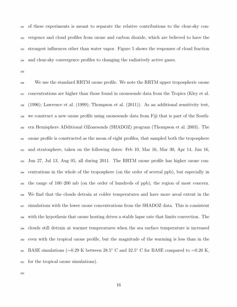
We use the standard RRTM ozone profile. We note the RRTM upper tropospheric ozone336

concentrations are higher than those found in ozonesonde data from the Tropics (Kley et al.337

(1996); Lawrence et al. (1999); Thompson et al. (2011)). As an additional sensitivity test,338

we construct a new ozone profile using ozonesonde data from Fiji that is part of the South-339

ern Hemisphere ADditional OZonesonds (SHADOZ) program (Thompson et al. 2003). The340

ozone profile is constructed as the mean of eight profiles, that sampled both the troposphere341

and stratosphere, taken on the following dates: Feb 10, Mar 16, Mar 30, Apr 14, Jun 16,342

Jun 27, Jul 13, Aug 05, all during 2011. The RRTM ozone profile has higher ozone con-343

centrations in the whole of the troposphere (on the order of several ppb), but especially in344

the range of 100–200 mb (on the order of hundreds of ppb), the region of most concern.345

We find that the clouds detrain at colder temperatures and have more areal extent in the346

simulations with the lower ozone concentrations from the SHADOZ data. This is consistent347

with the hypothesis that ozone heating drives a stable lapse rate that limits convection. The348

clouds still detrain at warmer temperatures when the sea surface temperature is increased349

even with the tropical ozone profile, but the magnitude of the warming is less than in the350

BASE simulations (∼0.29 K between 28.5◦ C and 32.5◦ C for BASE compared to ∼0.20 K,351

for the tropical ozone simulations).352

353

16

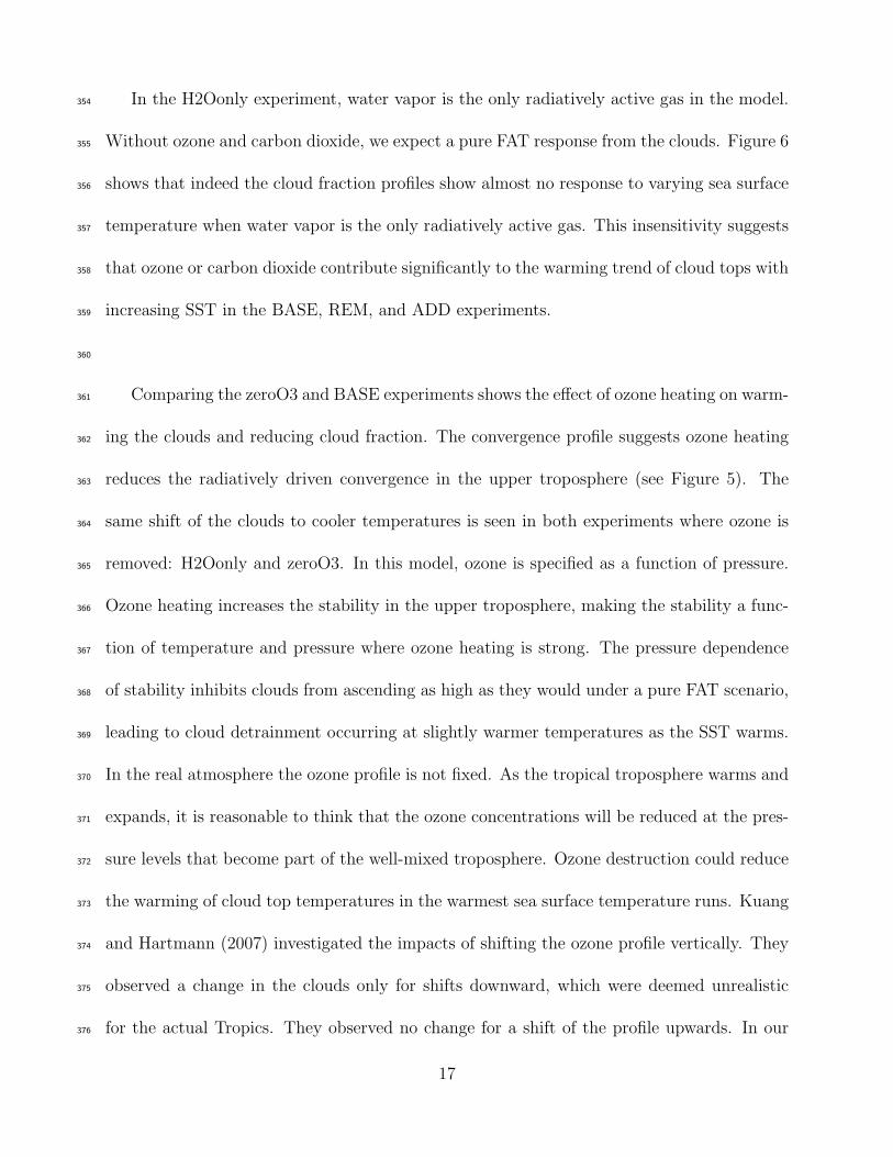
In the H2Oonly experiment, water vapor is the only radiatively active gas in the model.354

Without ozone and carbon dioxide, we expect a pure FAT response from the clouds. Figure 6355

shows that indeed the cloud fraction profiles show almost no response to varying sea surface356

temperature when water vapor is the only radiatively active gas. This insensitivity suggests357

that ozone or carbon dioxide contribute significantly to the warming trend of cloud tops with358

increasing SST in the BASE, REM, and ADD experiments.359

360

Comparing the zeroO3 and BASE experiments shows the effect of ozone heating on warm-361

ing the clouds and reducing cloud fraction. The convergence profile suggests ozone heating362

reduces the radiatively driven convergence in the upper troposphere (see Figure 5). The363

same shift of the clouds to cooler temperatures is seen in both experiments where ozone is364

removed: H2Oonly and zeroO3. In this model, ozone is specified as a function of pressure.365

Ozone heating increases the stability in the upper troposphere, making the stability a func-366

tion of temperature and pressure where ozone heating is strong. The pressure dependence367

of stability inhibits clouds from ascending as high as they would under a pure FAT scenario,368

leading to cloud detrainment occurring at slightly warmer temperatures as the SST warms.369

In the real atmosphere the ozone profile is not fixed. As the tropical troposphere warms and370

expands, it is reasonable to think that the ozone concentrations will be reduced at the pres-371

sure levels that become part of the well-mixed troposphere. Ozone destruction could reduce372

the warming of cloud top temperatures in the warmest sea surface temperature runs. Kuang373

and Hartmann (2007) investigated the impacts of shifting the ozone profile vertically. They374

observed a change in the clouds only for shifts downward, which were deemed unrealistic375

for the actual Tropics. They observed no change for a shift of the profile upwards. In our376

17

experiments, removing ozone allows the cloud to rise to lower pressures nearly isothermally377

as the sea surface temperature increases.378

379

The H2O+O3 experiment further demonstrates the effect of ozone. The inclusion of380

ozone is sufficient to create the slight warming of clouds with increasing sea surface tem-381

perature. Assuming the radiative effects of nitrous oxide, oxygen, and methane are small,382

the H2O+O3 case also gives some insight into the effect of carbon dioxide in our simula-383

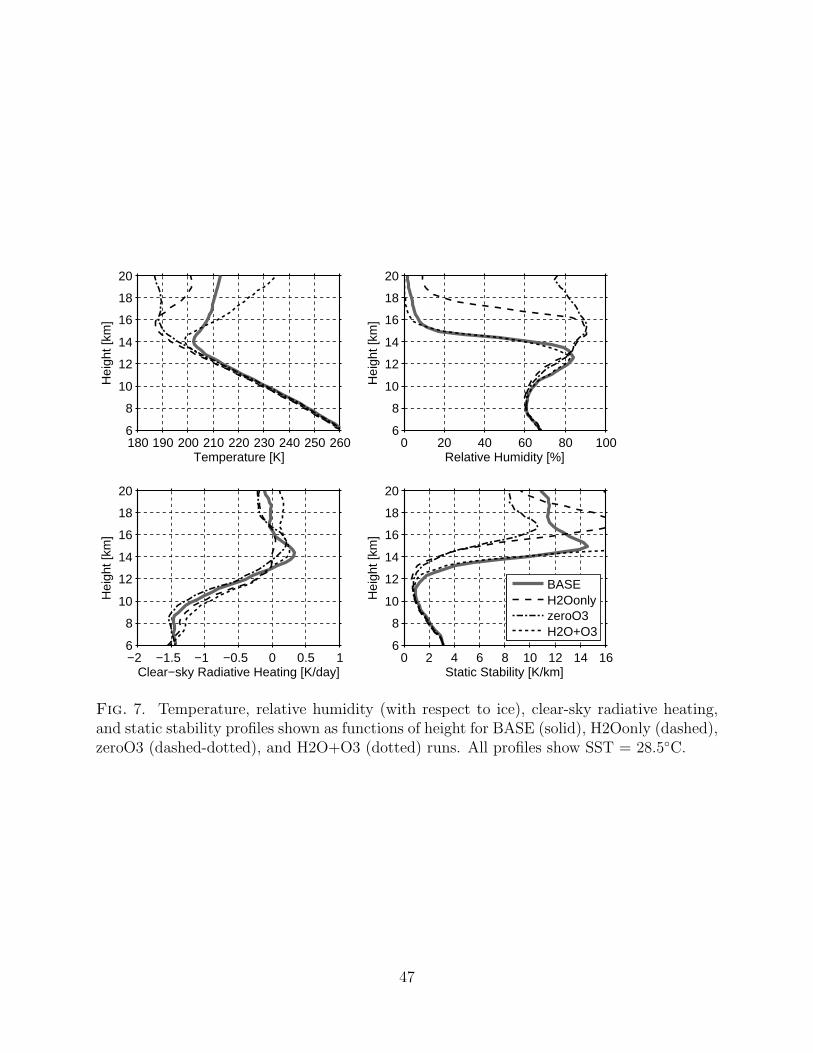
tions. Figure 5 shows that carbon dioxide warms the clouds. More specifically, Figure 7384

shows that the presence of carbon dioxide keeps the cold point from getting as cold as when385

carbon dioxide is removed (compare BASE with H2O+O3). Thus, the upper troposphere386

is actually less stable without carbon dioxide than with it. This interpretation is consistent387

with the increase in radiatively-driven convergence at higher altitudes when carbon dioxide388

is removed. The decrease in stability allows the clouds to rise to colder temperatures. While389

the upper troposphere is colder, the stratosphere is substantially warmer without carbon390

dioxide present as expected.391

392

Stratospheric water vapor concentrations are largely controlled by the cold point temper-393

ature and methane chemistry (Solomon et al. 2010). The cold point temperature is sensitive394

to sea surface temperature, ozone, and large-scale ascent (Oman et al. 2008) as well as con-395

vection (Kuang and Bretherton 2004). Because our model does not include a Brewer-Dobson396

circulation or methane chemistry, we cannot accurately predict the stratospheric water va-397

por value, so fixing its concentration for these experiments is necessary. As a simple test398

of the role of stratospheric water vapor, we double its concentration to 7 ppmv. Clouds in399

18

the 2xqv experiment detrain at a slightly warmer temperature than the BASE experiment400

(not shown). Kuang and Hartmann (2007) also performed a doubled stratospheric water401

vapor experiment (using a different radiative transfer code than we use). Their results show402

a similar slight warming of the clouds due to the increased water vapor.403

404

5. Radiative effects of cloud405

We next investigate the clouds’ radiative impact on their own evolution in our model.406

To do this, we remove the effect of cloud on radiative transfer. In the INVCLD simulations,407

the clear-sky flux and heating rate calculations are used to compute the tendencies for liquid408

water/ice moist static energy — the model’s prognostic energy quantity. In other words, the409

clouds do not contribute to the radiative heating in the model. If the detrainment level of the410

clouds does not align with the clear-sky convergence level when the clouds are invisible, then411

the radiative interaction of the clouds must be an important factor in determining that level.412

Again, we specify the same three sea surface temperatures for this experiment and examine413

the temperature profiles of the cloud fraction and clear-sky convergence. We find that the414

cloud levels remain consistent with that of the clear-sky convergence. Also, the cloud top415

temperatures for the INVCLD are similar to those of the BASE experiments. Two possible416

explanations for the insensitivity of the cloud top temperature to radiative effects of clouds417

immediately come to mind. First, clouds only appear where clear-sky radiative convergence418

drives cloud formation, so clouds cannot change their detrainment level. Second, whatever419

radiative impact clouds may have is being canceled by something else. McFarlane et al.420

19

(2007) have shown that clouds have non-negligible heating rates in the upper troposphere421

and it is reasonable to expect that these heating rates influence the clear-sky region. In the422

model, clear-sky cooling increases when the radiative effects of clouds are eliminated, seen423

in Figure 8. This additional cooling, however, is balanced by a strengthening of stability,424

which results in the convergence, and hence the clouds, remaining at the same level. It is425

perhaps not surprising that the clouds have little effect on their detrainment temperature426

in this model simply because the cloud fraction is small. The total cloud cover of clouds427

with tops colder than 265 K is about 0.12 for the BASE experiment with SST=28.5◦C. High428

cloud (tops higher than 440 mb) fraction is roughly 40–50% in convective regions estimated429

from MODIS satellite retrievals (Hong et al. 2007).430

431

The cloud fraction for the INVCLD experiment decreases compared to the BASE ex-432

periment. To investigate this effect further, we split the cloud fraction into three optical433

depth (τ) categories as in Kubar et al. (2007): thin (τ < 4), anvil (4 < τ < 32), and434

thick (τ > 32). Looking at Figure 9 it is apparent that the INVCLD experiment has fewer435

thin clouds than the BASE experiment. The thick and anvil cloud fractions are greater436

for the INVCLD experiments, suggesting something is inhibiting the clouds from spread-437

ing and thinning out. Garrett et al. (2005) proposed absorption of thermal radiation at438

cloud base and emission at cloud top spread anvil cirrus by creating density currents in the439

cloud. The spread they calculated using this method matched the Cirrus Regional Study440

of Tropical Anvils and Cirrus Layers–Florida Area Cirrus Experiment (CRYSTAL-FACE)441

observations (Garrett et al. 2005). Cirrus were shown to spread in a cloud resolving model442

due to thermal radiation absorption at cloud base and emission at cloud top (Krueger and443

20

Zulauf (2005); Garrett et al. (2006)). Tropical tropopause layer (TTL) cirrus have been444

shown to self-maintain themselves through radiative interactions (Durran et al. 2009; Dinh445

et al. 2010). Durran et al. (2009) showed that the radiative heating of thin TTL cirrus446

causes them to rise, and the resulting circulation, pulling air in toward the bottom and447

pushing air out toward the top, spreads the cloud. In the INVCLD experiment, we remove448

the heating and cooling for the cloud and thus remove the mechanisms for forming (Garrett449

et al. 2005) and maintaining (Durran et al. 2009) a larger fractional coverage of thin cirrus.450

Although our model has coarser resolution than the models used by Garrett et al. (2005) or451

Durran et al. (2009), their results are in agreement with those from our INVCLD experiment.452

453

6. Cloud-weighted temperature454

We quantify the changes in the profiles by determining the cloud-weighted and convergence-455

weighted temperatures. This is done similar to Kubar et al. (2007):456

TC =

∫ 245K

TcpC × T dT∫ 245K

TcpC dT

(7)457

Here, C is replaced with either the convergence or cloud fraction profile and Tcp is the458

cold point tropopause temperature. The upper limit is arbitrary. We select 245 K because459

it corresponds roughly to the level where longwave cooling begins to decline toward zero in460

our model.461

462

21

The cloud-fraction-weighted temperatures are plotted with respect to their correspond-463

ing convergence-weighted temperatures in Figure 10. The weighted temperature captures464

more than just the cloud tops, since the cloud fraction is weighted lower in the cloud and465

clear-sky convergence marks the top of the well-mixed convective layer and the beginning466

of the tropical tropopause layer (TTL). Thus, it should not be expected that Tconv = Tcld.467

Nonetheless, we expect that convergence-weighted and cloud-fraction-weighted temperatures468

will change in parallel. For example, increases (decreases) in water vapor’s ability to cool469

the atmosphere lead to lower (higher) weighted temperatures. Figure 10 shows warming of470

the clouds with increasing sea surface temperature for all of the experiments with ozone, and471

unchanging cloud temperatures with increasing SST for those experiments without ozone.472

For example, the H2Oonly case varies the least for both convergence- and cloud-weighted473

temperature (<0.5◦C) while the cases with ozone vary by about 2◦C for a 4◦C change in SST.474

475

Table 2 shows the differences in the weighted temperatures between SST=32.5◦C and476

SST=28.5◦C for each experiment. The increase in convergence-weighted and cloud-weighted477

temperatures are smallest for the experiments without ozone and in the case with doubled478

stratospheric water vapor. BASE has a small change in cloud-weighted temperature as well.479

The final column of Table 2 shows the change in the temperature where the domain-mean480

cloud fraction is highest (for high cloud only). Table 2 shows an increase in temperature of481

the cloud fraction peak of about 1.5–2 K for all experiments except H2Oonly and BIG.482

483

We next address whether there is statistical significance of the differences between cloud484

fraction profiles for different sea surface temperatures. The model output cloud fraction485

22

profiles are averaged over 2.5 days. The autocorrelation of each 2.5 day mean is used to get486

the effective number of degrees of freedom following Bretherton et al. (1999). A t-statistic487

is then used to attribute significance at the 95% level. For most experiments, a 4◦change488

in SST creates a significant difference in cloud fraction, while a 2◦change in SST does not489

(not shown). The experiments that show no difference for all three sea surface temperatures490

are those without ozone (H2Oonly and zeroO3), 2xqv, and BIG. The upper tropospheric491

cloud temperatures are invariant to sea surface temperature when ozone is not present in492

the simulation, as expected.493

7. Latent heating494

So far we have limited the discussion to changes in the radiative heating caused by changes495

in concentrations of radiatively active gases and the radiative effects of clouds. We now test496

whether we can change the cloud temperature by modifying the latent energy available to497

raise parcels. Condensational heating decreases with the saturation vapor pressure in the498

cold upper troposphere. By giving parcels greater energy, we test whether a drop off in499

condensational heating controls cloud top temperature, rather than the radiative relaxation.500

501

In the 2xLf experiments, everything is identical to the BASE experiments except that502

we double the latent heat of fusion. The cloud profile does not shift to colder temperatures.503

In fact, it shifts to slightly warmer temperatures, as compared to BASE, mostly because the504

cloud fraction decreases in the upper troposphere (not shown). The same increase in cloud505

top temperature with increasing sea surface temperature is seen with the 2xLf experiment506

23

(Figure 11). Moreover, static stability increases compared to the BASE runs resulting from507

the greater release of latent heat per unit of condensation. This causes the radiatively-driven508

convergence to decrease and its profile to shift toward warmer temperatures (not shown),509

leading to warmer anvil tops with lower fractional cloud cover. Thus, a decrease in latent510

heating as the air becomes colder higher up in the troposphere does not seem to be the reason511

that anvil clouds have a nearly constant temperature in these simulations. The invariance of512

the detrainment temperature of the clouds to the latent heat of fusion is consistent with the513

notion that cooling by radiative emission to maintain a convectively favorable environment514

is the primary control of cloud temperature in the tropical upper troposphere.515

516

8. Self-aggregation of clouds517

We have relied on the conceptual model of a dynamic circulation between the clear- and518

cloudy-sky regions as described by Hartmann and Larson (2002), yet the small model domain519

with its random, “popcorn” convection pattern does not show a well organized circulation520

pattern. We can create an organized circulation in the model if we allow self-aggregation of521

the clouds to occur. It has been shown in models that RCE can be maintained while cumulus522

convection self-aggregates or bunches together in the domain (Held et al. 1993; Bretherton523

et al. 2005). The process of self-aggregation causes the domain to shift to a higher moist adia-524

bat (than in the unaggregated case) due to the higher moist static energy air in the boundary525

layer of the convective region as shown by Bretherton et al. (2005). Self-aggregation also526

causes a drying of the non-convective region. One might expect that this drying could have a527

24

similar effect to the REM experiment. Held et al. (1993) explained self-aggregation through528

the memory convection leaves in the moisture field, in which future convection rises more529

easily where mid-tropospheric moisture is higher. The self-aggregation anomaly is sensitive530

to a number of factors (many of which are outlined by Bretherton et al. (2005)). For exam-531

ple, changing domain size and resolution is sufficient to determine whether self-aggregation532

occurs. Self-aggregation does not occur in the SAM model with the 96 × 96 km2 domain533

and 1 km resolution. Following Bretherton et al. (2005), we achieve self-aggregation using a534

domain size of 576× 576 km2 with 3 km resolution. Self-aggregation has direct parallels to535

the intertropical convergence zone (ITCZ), in that a large-scale circulation occurs between536

the clear- and cloudy-sky regions with subsidence in the clear-sky region and rising motion537

in the cloudy-sky region.538

539

The self-aggregation process occurs during model spin up, but requires a longer spin up540

time (75 days) than the small domain experiments (50 days) shown in previous sections541

(see Table 1). With self-aggregation occurring in the model, we apply the same removing542

and adding of water vapor (see equations (2) and (4), respectively). To save computation543

time, the modification experiments — BREM and BADD (the same as REM and ADD,544

respectively, but for an aggregated cloud field) — are initialized with the end of the BIG545

experiment such that the clouds are already aggregated. The adjustment to a new radiative-546

convective equilibrium profile takes 25 days. The model is run an additional 50 days for the547

statistical profiles shown.548

549

Self-aggregation causes the clouds to rise to higher altitudes. The domain mean cloud550

25

fraction, however, is smaller for the self-aggregated experiments compared to the non-551

aggregated ones. While the BIG experiments with sea surface temperatures of 30.5◦C and552

32.5◦C showed the same near constancy of cloud-weighted temperature with SST as the553

BASE case (Figure 10), the cloud fraction profiles do not show an increase of cloud top554

temperature for increasing SST (see Figure 12). The increase in cloud-weighted tempera-555

ture is due to an increase in mid-level clouds, relative to the peak amount, which biases the556

weighted temperature value. The BREM and BADD experiments behave like the REM and557

ADD experiments: the clouds detrain at warmer temperatures in the BREM experiments558

and colder temperatures in the BADD experiment.559

560

We also examine the humidity profiles between the moist and dry regions to see if there is561

any evidence that the drying of the clear-sky region is influencing the cloud temperature. To562

sample the wet and dry regions, we divide the domain into a 16×16 horizontal grid and take563

the wettest and driest quartiles of that grid. Here, “wettest” and “driest” are the highest564

and lowest mean water vapor paths, respectively. Though the dry region has substantially565

less water vapor in the mid-troposphere, the water vapor profiles of the wet and dry regions566

converge in the upper troposphere (not shown). The uniform upper level humidity suggests567

that detrainment and advection of water from the convective region covers the entire do-568

main. Water vapor advected to the clear-sky region allows for stronger cooling in the upper569

troposphere. The temperature and stability profiles in the clear and convective regions are570

identical due to gravity waves (“convective adjustment”).571

572

Figure 13 shows the mass fluxes (calculated simply as the product of vertical velocity573

26

and density for each grid space) for the BIG experiments compared with BASE. Mass fluxes574

are averaged over cloudy columns as well as the unsaturated environment (the mass fluxes575

are equal and opposite by construction since no mass leaves or enters the model domain). A576

cloudy column is one such that the column averaged cloud (water + ice) amount surpasses577

5 × 10−4 kg/kg (roughly twice the domain averaged column amount). While the mass flux578

in the middle troposphere is less in the self-aggregated experiment compared to BASE, it is579

greater in the upper troposphere near the cold point tropopause. Less mass flux shows that580

the organized large-scale circulation (with the updrafts grouped together and subsidence581

region surrounding them) in the aggregated cloud field is weaker than the mesoscale circu-582

lations (the unorganized updraft- and subsidence-regions in the small domain simulations)583

created in the non-aggregated experiments. Changing the threshold used for determining584

the cloudy skies did not qualitatively alter the results. The local maximum in mass flux585

at ∼10 km in the BASE case suggests a secondary circulation. For the mass flux to in-586

crease with altitude, the vertical velocity must also increase with altitude — since density587

decreases. An increasing vertical velocity suggests convergence in the horizontal (note that588

this convergence is in the cloudy-sky and is below the level of anvil detrainment). The BIG589

mass flux profiles suggest that convection regularly approaches the height of the cold point590

when aggregated (14, 15, and 16 km for SST = 28.5◦C, 30.5◦C, and 32.5◦C, respectively).591

Overshooting convection can warm the cold point by mixing down high potential energy air.592

The cold point temperature is 5 K warmer in the BIG experiment than for the BASE ex-593

periment. The warmer upper tropospheric temperatures in the aggregated experiment allow594

for greater water vapor cooling. Stronger water vapor cooling cancels the ozone warming to595

make the clouds rise isothermally in our aggregated experiments in response to SST increases.596

27

597

9. Conclusions598

The sensitivity of tropical cloud top temperature to radiative cooling by water vapor is599

tested using the SAM 3D cloud resolving model. We demonstrate that changes in the ability600

of water vapor to cool the air have a direct influence on the cloud top temperature. Weakened601

cooling increases cloud top temperatures, and strengthened cooling decreases cloud top tem-602

peratures. These results agree with expectations from the Fixed Anvil Temperature (FAT)603

hypothesis proposed by Hartmann and Larson (2002) as well as model results from Kuang604

and Hartmann (2007) and observations by Kubar et al. (2007). Cloud top temperature is605

shown to be nearly insensitive to sea surface temperature. A slight warming of the clouds606

is shown for increasing sea surface temperatures, attributed to an increase in static stability607

in the upper troposphere (which agrees with observations from Chae and Sherwood (2010)608

as well as an analysis of GCM results by Zelinka and Hartmann (2010)). A slight decrease609

of cloud fraction is also shown for increasing sea surface temperatures. The responses to610

sea surface temperature changes are minor compared to those due to changes in radiative611

cooling by water vapor, suggesting water vapor cooling controls the cloud top temperature.612

This produces a positive longwave cloud feedback since cloud emission temperature remains613

roughly constant as the surface warms.614

615

The radiative impacts of ozone, carbon dioxide, and the clouds are shown to be secondary616

to that of water vapor. The simulations with and without ozone suggest that the stability in-617

28

crease caused by radiative heating of ozone causes the slight warming of the clouds observed618

with increasing sea surface temperature. Carbon dioxide increases the stability of the upper619

troposphere, causing clouds to detrain at warmer temperatures. Cloud radiative heating620

has little effect on determining the temperature of anvil detrainment in our experiments.621

While the rapid decline with height in water vapor in the upper troposphere is shown to622

have the strongest influence on the heating and stability profile, stratospheric water vapor623

plays a non-trivial role in determining the heating profile as well as the stability of the upper624

tropical troposphere.625

626

Further experiments test if declining condensational heating is a strong constraint on627

cloud top temperature. Doubling the latent heat of fusion stabilizes the upper-most layers628

of the troposphere, inhibiting convection from reaching temperatures as cold as those seen629

in the BASE simulations, and reducing the high cloud amount. With a large domain, con-630

vection is able to self-aggregate, but the weak sensitivity of cloud temperatures to surface631

temperature is very similar to that of the unaggregated cases. In the presence of an organized632

circulation, such as that caused by the simulation reaching a state of self-aggregation, the633

same control of cloud top temperature by emission from water vapor remains. In fact, con-634

vective organization creates a stronger coupling of the clear- and cloudy-sky regions keeping635

the clouds at a fixed temperature. The circulation’s effect on the clouds is stronger than the636

small heating due to fixed ozone seen in the unaggregated experiments.637

638

For our simulations, changing sea surface temperature warms the clouds because the639

ozone profile is a fixed function of pressure. A fixed ozone profile is probably not a realis-640

29

tic feature of the Tropics. The effect of ozone may change as the troposphere warms and641

expands and vertical mixing reduces ozone concentrations at pressure levels that become642

part of the well-mixed troposphere (Kley et al. 1996). The simulations using the ozone643

profile constructed from SHADOZ data also show that lowering upper tropospheric ozone644

concentrations causes the clouds to detrain at colder temperatures. Increasing stratospheric645

water vapor increases the cloud top temperature in our simulations. Stratospheric water646

vapor (as measured by balloon over Boulder) has increased since 1980 (Hurst et al. 2011).647

However, the increase is not monotonic and there are multiple periods of decrease in the648

record. Our model does not include any supra-domain-scale (outside of the domain of the649

simulation) circulation, but we know that adiabatic processes can influence the stability as650

well as the cold point tropopause temperature. In addition, large-scale motions can change651

the humidity profile of the atmosphere, and thus, the radiative cooling profile. Quantifying652

the effects of factors beyond our RCE model to the clear-sky convergence will be important653

for determining the energy budget of the Tropics.654

655

Acknowledgments.656

The authors wish to thank Peter Blossey for his help running the SAM cloud resolving657

model, as well as Thomas Ackerman and Christopher Bretherton for helpful discussions,658

and the reviewers for their comments. The work was supported by the Atmospheric and659

Geospace Sciences Division of the National Science Foundation Grant AGS-0960497660

30

661

REFERENCES662

Bretherton, C. S., P. N. Blossey, and M. Khairoutdinov, 2005: An energy-balance analysis663

of deep convective self-aggregation above uniform sst. J. Atmos. Sci., 62, 4273–4292.664

Bretherton, C. S., M. Widmann, V. P. Dymnikov, J. M. Wallace, and I. Blade, 1999: The665

effective number of spatial degrees of freedom of a time-varying field. J. Climate, 12 (7),666

1990–2009.667

Chae, J. H. and S. C. Sherwood, 2010: Insights into cloud-top height and dynamics from the668

seasonal cycle of cloud-top heights observed by misr in the west pacific region. J. Atmos.669

Sci., 67, 248–261, doi:10.1175/2009JAS3099.1.670

Dinh, T. P., D. R. Durran, and T. P. Ackerman, 2010: Maintenance of tropical tropopause671

layer cirrus. J. Geophys. Res.-Atmospheres, 115, D02 104.672

Durran, D. R., T. Dinh, M. Ammerman, and T. Ackerman, 2009: The mesoscale dynamics673

of thin tropical tropopause cirrus. J. Atmos. Sci., 66 (9), 2859–2873.674

Eitzen, Z. A., K. Xu, and T. Wong, 2009: Cloud and radiative characteristics of tropical675

deep convective systems in extended cloud objects from ceres observations. J. Climate,676

22, 5983–6000, doi:10.1175/2009JCLI3038.1.677

Eyring, V., et al., 2006: Assessment of temperature, trace species, and ozone in chemistry-678

climate model simulations of the recent past. J. Geophys. Res.-Atmospheres, 111 (D22),679

D22 308.680

31

Fu, Q. and K. N. Liou, 1992: On the correlated k-distribution method for radiative-transfer681

in nonhomogeneous atmospheres. J. Atmos. Sci., 49 (22), 2139–2156.682

Garrett, T. J., M. A. Zulauf, and S. K. Krueger, 2006: Effects of cirrus near the tropopause683

on anvil cirrus dynamics. Geophys. Res. Lett., 33 (17), L17 804.684

Garrett, T. J., et al., 2005: Evolution of a florida cirrus anvil. J. Atmos. Sci., 62 (7),685

2352–2372.686

Hartmann, D. L., J. R. Holton, and Q. Fu, 2001: The heat balance of the tropical tropopause,687

cirrus, and stratospheric dehydration. Geophys. Res. Lett., 28, doi:10.1029/2000GL012833.688

Hartmann, D. L. and K. Larson, 2002: An important constraint on tropical cloud - climate689

feedback. Geophys. Res. Lett., 29, doi:10.1029/2002GL015835.690

Held, I. M., R. S. Hemler, and V. Ramaswamy, 1993: Radiative convective equilibrium with691

explicit 2-dimensional moist convection. J. Atmos. Sci., 50, 3909–3927.692

Hong, G., P. Yang, B.-C. Gao, B. A. Baum, Y. X. Hu, M. D. King, and S. Platnick, 2007:693

High cloud properties from three years of modis terra and aqua collection-4 data over the694

tropics. J. Appl. Met. Climatol., 46 (11), 1840–1856.695

Houze, R. A. and A. K. Betts, 1981: Convection in gate. Rev. Geophys., 19, 541–576.696

Hurst, D. F., S. J. Oltmans, H. Voemel, K. H. Rosenlof, S. M. Davis, E. A. Ray, E. G.697

Hall, and A. F. Jordan, 2011: Stratospheric water vapor trends over boulder, colorado:698

Analysis of the 30 year boulder. J. Geophys. Res.-Atmospheres, 116, D02 306, doi:10.1029/699

2010JD015065.700

32

Khairoutdinov, M. F. and D. A. Randall, 2003: Cloud resolving modeling of the arm summer701

1997 iop: Model formulation, results, uncertainties, and sensitivities. J. Atmos. Sci., 60,702

607–625.703

Kley, D., P. J. Crutzen, H. G. J. Smit, H. Vomel, S. J. Oltmans, H. Grassl, and V. Ra-704

manathan, 1996: Observations of Near-Zero Ozone Concentrations Over the Convective705

Pacific: Effects on Air Chemistry. Science, 274 (5285), 230–233, doi:10.1126/science.274.706

5285.230.707

Krueger, S. and M. Zulauf, 2005: Radiatively-Induced Anvil Spreading. Proceedings of the708

Fifteenth Atmospheric Radiation Measurement (ARM) Science Team Meeting, Daytona709

Beach, Florida, DOE, URL http://www.arm.gov/publications/proceedings/conf15/710

extended_abs/krueger_sk.pdf.711

Kuang, Z. and C. S. Bretherton, 2004: Convective influence on the heat balance of the712

tropical tropopause layer: A cloud-resolving model study. J. Atmos. Sci., 61, 2919–2927.713

Kuang, Z. and D. L. Hartmann, 2007: Testing the fixed anvil temperature hypothesis in a714

cloud-resolving model. J. Climate, 20, 2051–2057.715

Kubar, T. L., D. L. Hartmann, and R. Wood, 2007: Radiative and convective driving of716

tropical high clouds. J. Climate, 20, 5510–5526, doi:10.1175/2007JCLI1628.1.717

Lawrence, M., P. Crutzen, and P. Rasch, 1999: Analysis of the CEPEX ozone data using a718

3D chemistry-meteorology model. Quart. J. Roy. Meteor. Soc., 125 (560), 2987–3009.719

McFarlane, S. A., J. H. Mather, and T. P. Ackerman, 2007: Analysis of tropical radiative720

33

heating profiles: A comparison of models and observations. J. Geophys. Res.-Atmospheres,721

112 (D14), D14 218.722

Mlawer, E. J., S. J. Taubman, P. D. Brown, M. J. Iacono, and S. A. Clough, 1997: Radiative723

transfer for inhomogeneous atmospheres: Rrtm, a validated correlated-k model for the724

longwave. J. Geophys. Res.-Atmospheres, 102, 16 663–16 682.725

Oman, L., D. W. Waugh, S. Pawson, R. S. Stolarski, and J. E. Nielsen, 2008: Understanding726

the changes of stratospheric water vapor in coupled chemistry-climate model simulations.727

J. Atmos. Sci., 65 (10), 3278–3291.728

Pawson, S., et al., 2000: The gcm-reality intercomparison project for sparc (grips): Scientific729

issues and initial results. Bull. Amer. Meteor. Soc., 81 (4), 781–796.730

Rind, D. and P. Lonergan, 1995: Modeled impacts of stratospheric ozone and water-vapor731

perturbations with implications for high-speed civil transport aircraft. J. Geophys. Res.-732

Atmospheres, 100 (D4), 7381–7396.733

Solomon, S., K. H. Rosenlof, R. W. Portmann, J. S. Daniel, S. M. Davis, T. J. Sanford,734

and G.-K. Plattner, 2010: Contributions of stratospheric water vapor to decadal changes735

in the rate of global warming. Science (New York, N.Y.), 327 (5970), 1219–23, doi:736

10.1126/science.1182488, URL http://www.ncbi.nlm.nih.gov/pubmed/20110466.737

Thompson, A. M., A. L. Allen, S. Lee, S. K. Miller, and J. C. Witte, 2011: Gravity738

and Rossby wave signatures in the tropical troposphere and lower stratosphere based on739

Southern Hemisphere Additional Ozonesondes (SHADOZ), 19982007. J. Geophys. Res.,740

116 (D5), 1998–2007, doi:10.1029/2009JD013429.741

34

Thompson, A. M., et al., 2003: Southern Hemisphere Additional Ozonesondes (SHADOZ)742

1998-2000 tropical ozone climatology 1. Comparison with Total Ozone Mapping Spectrom-743

eter (TOMS) and ground-based measurements. J. Geophys. Res., 108 (D2), 1998–2000,744

doi:10.1029/2001JD000967.745

Tompkins, A. M. and G. C. Craig, 1999: Sensitivity of tropical convection to sea surface746

temperature in the absence of large-scale flow. J. Climate, 12, 462–476.747

Xu, K., T. Wong, B. A. Wielicki, L. Parker, B. Lin, Z. A. Eitzen, and M. Branson, 2007:748

Statistical analyses of satellite cloud object data from ceres. part ii: Tropical convective749

cloud objects during 1998 el nino and evidence for supporting the fixed anvil temperature750

hypothesis. J. Climate, 20, 819–842, doi:10.1175/JCLI4069.1.751

Zelinka, M. D. and D. L. Hartmann, 2010: Why is longwave cloud feedback positive? J.752

Geophys. Res.-Atmospheres, 115, D16 117.753

Zelinka, M. D. and D. L. Hartmann, 2011: The observed sensitivity of high clouds to mean754

surface temperature anomalies in the tropics. J. Geophys. Res., 116 (D23), doi:10.1029/755

2011JD016459.756

35

List of Tables757

1 List of experiments. Water vapor removal/addition refers to alterations to the758

water vapor concentration passed to the radiative transfer code. Note that759

all runs are performed for three different sea surface temperatures (28.5◦C,760

30.5◦C, 32.5◦C) except for experiments BREM and BADD (both done only761

at SST=28.5◦C; see section 8). 37762

2 Difference in cloud-weighted temperature (∆Tcld), convergence-weighted tem-763

perature (∆Tconv), and temperature of the cloud fraction peak (Peak CT)764

between SST=32.5◦and SST=28.5◦. 38765

36

Table 1. List of experiments. Water vapor removal/addition refers to alterations to thewater vapor concentration passed to the radiative transfer code. Note that all runs areperformed for three different sea surface temperatures (28.5◦C, 30.5◦C, 32.5◦C) except forexperiments BREM and BADD (both done only at SST=28.5◦C; see section 8).

Name Domain Size Resolution Duration AveragedDays

Description

BASE 96×96 km2 1 km 100 days 50–100 No modificationREM 96×96 km2 1 km 100 days 50–100 Water vapor removal; T1=250 K

(see equation (2))ADD 96×96 km2 1 km 100 days 50–100 Water vapor addition; T1=250

K; T2=220 K; K=2 (see equa-tion (4))

H2Oonly 96×96 km2 1 km 100 days 50–100 Zero out all radiatively activegases except water vapor

zeroO3 96×96 km2 1 km 100 days 50–100 Zero out only ozoneH2O+O3 96×96 km2 1 km 100 days 50–100 Zero out all radiatively active

gases except water vapor andozone

2xqv 96×96 km2 1 km 100 days 50–100 Doubled stratospheric water va-por

INVCLD 96×96 km2 1 km 100 days 50–100 Clouds invisible to radiativetransfer model

2xLf 96×96 km2 1 km 100 days 50–100 Doubled latent heat of fusionBIG 576×576 km2 3 km 125 days 75–125 Large domain, self-aggregated

runBREM 576×576 km2 3 km 75 days 25–75 As in REM except large domain,

self-aggregated; initialized withend of BIG run so that self-aggregation has already takenplace

BADD 576×576 km2 3 km 75 days 25–75 As in ADD except large domain,self-aggregated; initialized withend of BIG run

37

Table 2. Difference in cloud-weighted temperature (∆Tcld), convergence-weighted tempera-ture (∆Tconv), and temperature of the cloud fraction peak (Peak CT) between SST=32.5◦andSST=28.5◦.

Experiment ∆Tcld ∆Tconv Peak CT

BASE 0.29 1.36 1.98REM 1.00 1.07 1.53ADD 0.93 1.19 2.03H2Oonly 0.26 0.58 -0.81zeroO3 -0.59 0.15 1.72H2O+O3 1.17 1.27 1.982xqv 0.09 1.15 1.82INVCLD 0.74 1.36 1.662xLf 1.01 1.42 1.97BIG 0.33 1.20 -1.41

38

List of Figures766

1 Water vapor modification diagram. The different lines show the BASE (solid),767

REM (dashed), and ADD (dashed-dotted). For both REM and ADD, T1 =768

250K and for ADD T2 = 220K and K = 2. 41769

2 Cloud fraction presented as functions of temperature. For each plot, lines770

show runs for SST = 28.5◦C (dashed), SST = 30.5◦C (solid), and SST =771

32.5◦C (dashed-dotted). 42772

3 Cloud fraction and clear-sky convergence shown for the BASE (solid), REM773

(dashed), and ADD (dashed-dotted)) runs. All plots show SST = 28.5◦C. 43774

4 Temperature, relative humidity (with respect to ice; using model predicted775

water vapor for all three experiments), clear-sky radiative heating, and static776

stability profiles shown as functions of height for BASE (solid), REM (dashed),777

and ADD (dashed-dotted). All profiles show SST = 28.5◦C. 44778

5 Cloud fraction and clear-sky convergence shown for H2Oonly (dashed), zeroO3779

(dashed-dotted), H2O+O3 (dotted), and BASE (solid) runs. All plots show780

SST = 28.5◦C. 45781

6 Cloud fraction presented as functions of temperature. For each plot, lines show782

runs for SST = 28.5◦C (dashed), SST = 30.5◦C (solid), and SST = 32.5◦C783

(dashed-dotted). BASE, SST=28.5◦C (gray, solid) is shown for comparison. 46784

39

7 Temperature, relative humidity (with respect to ice), clear-sky radiative heat-785

ing, and static stability profiles shown as functions of height for BASE (solid),786

H2Oonly (dashed), zeroO3 (dashed-dotted), and H2O+O3 (dotted) runs. All787

profiles show SST = 28.5◦C. 47788

8 BASE (solid, gray) and INVCLD (dashed, black) profiles for: (left) clear-sky789

convergence; (middle) clear-sky radiative heating; (right) static stability. All790

plots show SST = 28.5◦C. 48791

9 Cloud fraction separated by optical depth bins: thin (τ < 4), anvil (4 < τ <792

32), and thick (τ > 32). Both plots show SST = 28.5◦C. 49793

10 Convergence-weighted temperature on the x-axis; cloud fraction-weighted tem-794

perature on y-axis. For all symbols, the shading corresponds to SST = 28.5◦C795

(black), SST = 30.5◦C (gray), SST = 32.5◦C (white). 50796

11 Cloud fraction presented as functions of temperature for 2xLf case. Lines show797

runs for SST = 28.5◦C (dashed), SST = 30.5◦C (solid), and SST = 32.5◦C798

(dashed-dotted). BASE, SST=28.5◦C (gray, solid) is shown for comparison. 51799

12 Cloud fraction presented as functions of temperature for the BIG case. Lines800

show runs for SST = 28.5◦C (dashed), SST = 30.5◦C (solid), and SST =801

32.5◦C (dashed-dotted). BASE, SST=28.5◦C (gray, solid) is shown for com-802

parison. 52803

13 Mass fluxes for cloudy (positive) and unsaturated environment (negative) pre-804

sented as functions of height for BIG case. Lines show runs for SST = 28.5◦C805

(dashed), SST = 30.5◦C (solid), and SST = 32.5◦C (dashed-dotted). BASE,806

SST=28.5◦C (gray, solid) is shown for comparison. 53807

40

10−3

10−2

10−1

100

101

6

8

10

12

14

16

18

Height where T = 250 K

BASE

REM

ADD

Water Vapor [g/kg]

Hei

ght [

km]

Fig. 1. Water vapor modification diagram. The different lines show the BASE (solid), REM(dashed), and ADD (dashed-dotted). For both REM and ADD, T1 = 250K and for ADDT2 = 220K and K = 2.

41

0 0.04 0.08 0.12

190

205

220

235

250

265

Tem

pera

ture

[K]

BASE

Cloud Fraction0 0.04 0.08 0.12

190

205

220

235

250

265

REM

Cloud Fraction0 0.04 0.08 0.12

190

205

220

235

250

265

ADD

Cloud Fraction

Fig. 2. Cloud fraction presented as functions of temperature. For each plot, lines show runsfor SST = 28.5◦C (dashed), SST = 30.5◦C (solid), and SST = 32.5◦C (dashed-dotted).

42

0 0.04 0.08 0.12

190

205

220

235

250

265

Tem

pera

ture

[K]

Cloud Fraction

−0.5 0 0.5 1

190

205

220

235

250

265

Convergence [day−1]

REMADDBASE

REMADDBASE

Fig. 3. Cloud fraction and clear-sky convergence shown for the BASE (solid), REM(dashed), and ADD (dashed-dotted)) runs. All plots show SST = 28.5◦C.

43

0 20 40 60 80 1006

8

10

12

14

16

18

20

Hei

ght [

km]

Relative Humidity [%]180 190 200 210 220 230 240 250 2606

8

10

12

14

16

18

20

Hei

ght [

km]

Temperature [K]

0 2 4 6 8 10 12 14 166

8

10

12

14

16

18

20

Hei

ght [

km]

Static Stability [K/km]

−2 −1.5 −1 −0.5 0 0.5 16

8

10

12

14

16

18

20

Hei

ght [

km]

Clear−sky Radiative Heating [K/day]

BASEREMADD

Fig. 4. Temperature, relative humidity (with respect to ice; using model predicted watervapor for all three experiments), clear-sky radiative heating, and static stability profilesshown as functions of height for BASE (solid), REM (dashed), and ADD (dashed-dotted).All profiles show SST = 28.5◦C.

44

0 0.04 0.08 0.12

190

205

220

235

250

265

Tem

pera

ture

[K]

Cloud Fraction

−0.5 0 0.5 1

190

205

220

235

250

265

Convergence [day−1]

H2OonlyzeroO3H2O+O3BASE

H2OonlyzeroO3H2O+O3BASE

Fig. 5. Cloud fraction and clear-sky convergence shown for H2Oonly (dashed), zeroO3(dashed-dotted), H2O+O3 (dotted), and BASE (solid) runs. All plots show SST = 28.5◦C.

45

0 0.04 0.08 0.12

190

205

220

235

250

265

Tem

pera

ture

[K]

H2Oonly

Cloud Fraction0 0.04 0.08 0.12

190

205

220

235

250

265

zeroO3

Cloud Fraction0 0.04 0.08 0.12

190

205

220

235

250

265

H2O+O3

Cloud Fraction

Fig. 6. Cloud fraction presented as functions of temperature. For each plot, lines showruns for SST = 28.5◦C (dashed), SST = 30.5◦C (solid), and SST = 32.5◦C (dashed-dotted).BASE, SST=28.5◦C (gray, solid) is shown for comparison.

46

0 20 40 60 80 1006

8

10

12

14

16

18

20

Hei

ght [

km]

Relative Humidity [%]180 190 200 210 220 230 240 250 2606

8

10

12

14

16

18

20

Hei

ght [

km]

Temperature [K]

0 2 4 6 8 10 12 14 166

8

10

12

14

16

18

20

Hei

ght [

km]

Static Stability [K/km]

−2 −1.5 −1 −0.5 0 0.5 16

8

10

12

14

16

18

20

Hei

ght [

km]

Clear−sky Radiative Heating [K/day]

BASEH2OonlyzeroO3H2O+O3

Fig. 7. Temperature, relative humidity (with respect to ice), clear-sky radiative heating,and static stability profiles shown as functions of height for BASE (solid), H2Oonly (dashed),zeroO3 (dashed-dotted), and H2O+O3 (dotted) runs. All profiles show SST = 28.5◦C.

47

−0.5 0 0.5 1

190

205

220

235

250

265

Tem

pera

ture

[K]

Convergence [day−1]0 0.05 0.1 0.15 0.2

190

205

220

235

250

265

Tem

pera

ture

[K]

Static Stability [K/mb ]−1.8 −1.3 −0.8 −0.3 0.2

190

205

220

235

250

265

Tem

pera

ture

[K]

Radiative Heating [K/day ]

BASEINVCLD

Fig. 8. BASE (solid, gray) and INVCLD (dashed, black) profiles for: (left) clear-sky con-vergence; (middle) clear-sky radiative heating; (right) static stability. All plots show SST =28.5◦C.

48

0 0.01 0.02 0.03

190

215

240

265

Tem

pera

ture

[K]

Cloud Fractions

BASE

thinanvilthick

0 0.01 0.02 0.03

190

215

240

265

Cloud Fractions

INVCLD

thinanvilthick

Fig. 9. Cloud fraction separated by optical depth bins: thin (τ < 4), anvil (4 < τ < 32),and thick (τ > 32). Both plots show SST = 28.5◦C.

49

213 215 217 219 221 223 225 213221

223

225

227

229

231

221

♥♥

Convergence Weighted Temperature [K]

Clo

ud F

ract

ion

Wei

ghte

d T

empe

ratu

re [K

]

BASEREMADDH2OonlyzeroO3H2O+O32xqvINVCLD2xLfBIGBREM

♥ BADD

Fig. 10. Convergence-weighted temperature on the x-axis; cloud fraction-weighted temper-ature on y-axis. For all symbols, the shading corresponds to SST = 28.5◦C (black), SST =30.5◦C (gray), SST = 32.5◦C (white).

50

0 0.04 0.08 0.12

190

205

220

235

250

265

Tem

pera

ture

[K]

Cloud Fraction

Fig. 11. Cloud fraction presented as functions of temperature for 2xLf case. Lines showruns for SST = 28.5◦C (dashed), SST = 30.5◦C (solid), and SST = 32.5◦C (dashed-dotted).BASE, SST=28.5◦C (gray, solid) is shown for comparison.

51

0 0.04 0.08 0.12

190

205

220

235

250

265

Tem

pera

ture

[K]

Cloud Fraction

Fig. 12. Cloud fraction presented as functions of temperature for the BIG case. Lines showruns for SST = 28.5◦C (dashed), SST = 30.5◦C (solid), and SST = 32.5◦C (dashed-dotted).BASE, SST=28.5◦C (gray, solid) is shown for comparison.

52

−6 −4 −2 0 2 4 6

x 10−3

6

8

10

12

14

16

18

20

Mass Flux [kg m−2 s−1]

Hei

ght [

km]

Fig. 13. Mass fluxes for cloudy (positive) and unsaturated environment (negative) presentedas functions of height for BIG case. Lines show runs for SST = 28.5◦C (dashed), SST =30.5◦C (solid), and SST = 32.5◦C (dashed-dotted). BASE, SST=28.5◦C (gray, solid) isshown for comparison.

53