Boyce/DiPrima 9 ed, Ch 7.8: Repeated Eigenvalueszheng/ODE_09Fall/ch7_8.pdf · Boyce/DiPrima 9 th...
19
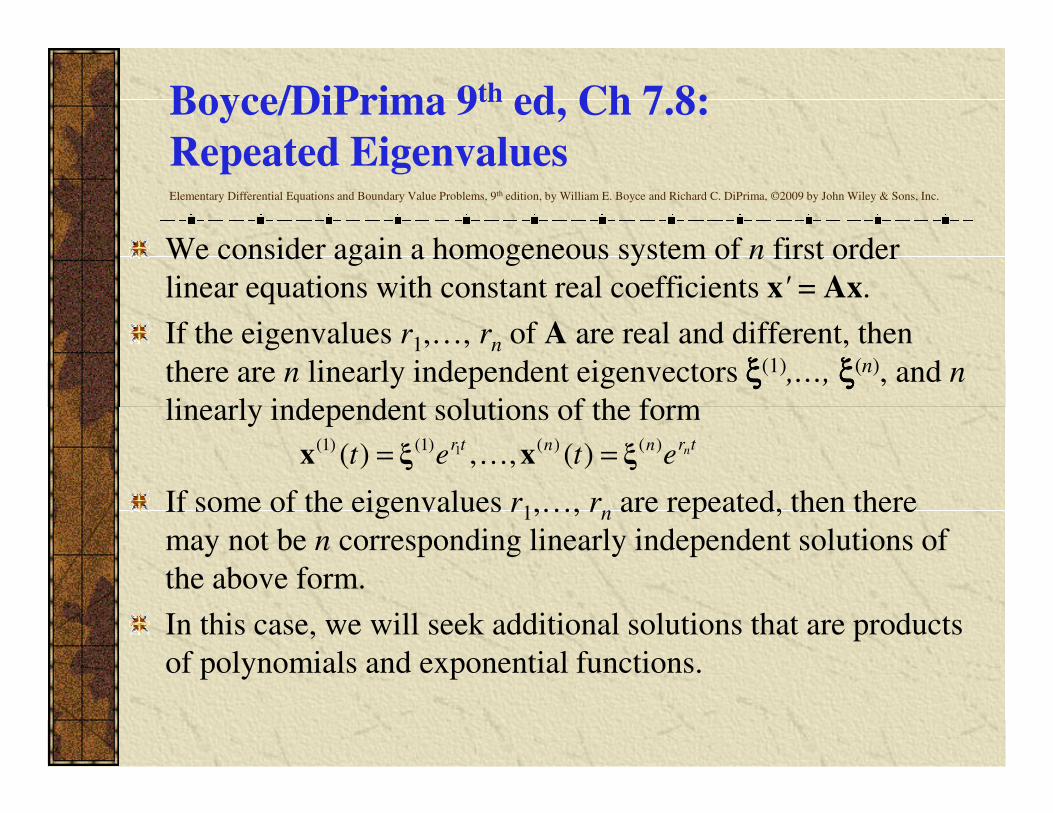
Boyce/DiPrima 9 th ed, Ch 7.8: Repeated Eigenvalues Elementary Differential Equations and Boundary Value Problems, 9 th edition, by William E. Boyce and Richard C. DiPrima, ©2009 by John Wiley & Sons, Inc. We consider again a homogeneous system of n first order linear equations with constant real coefficients x' = Ax. If the eigenvalues r 1 ,…, r n of A are real and different, then there are n linearly independent eigenvectors ξ ξ ξ (1) ,…, ξ ξ ξ (n) , and n linearly independent solutions of the form linearly independent solutions of the form If some of the eigenvalues r 1 ,…, r n are repeated, then there may not be n corresponding linearly independent solutions of the above form. In this case, we will seek additional solutions that are products of polynomials and exponential functions. t r n n t r n e t e t ) ( ) ( ) 1 ( ) 1 ( ) ( , , ) ( 1 ξ x ξ x = = …
Transcript of Boyce/DiPrima 9 ed, Ch 7.8: Repeated Eigenvalueszheng/ODE_09Fall/ch7_8.pdf · Boyce/DiPrima 9 th...
Boyce/DiPrima 9th ed, Ch 7.8:
Repeated EigenvaluesElementary Differential Equations and Boundary Value Problems, 9th edition, by William E. Boyce and Richard C. DiPrima, ©2009 by John Wiley & Sons, Inc.
We consider again a homogeneous system of n first order
linear equations with constant real coefficients x' = Ax.
If the eigenvalues r1,…, rn of A are real and different, then
there are n linearly independent eigenvectors ξξξξ(1),…, ξξξξ(n), and n
linearly independent solutions of the formlinearly independent solutions of the form
If some of the eigenvalues r1,…, rn are repeated, then there
may not be n corresponding linearly independent solutions of
the above form.
In this case, we will seek additional solutions that are products
of polynomials and exponential functions.
trnntr netet)()()1()1( )(,,)( 1 ξxξx == …

Example 1: Eigenvalues (1 of 2)
We need to find the eigenvectors for the matrix:
The eigenvalues r and ξξξξ eigenvectors satisfy the equatio
(A – rI ) ξξξξ=0 or
x
−=
31
11AAAA
(A – rI ) ξξξξ=0 or
To determine r, solve det(A-rI) = 0:
Thus r1 = 2 and r2 = 2.
22 )2(441)3)(1(31
11−=+−=+−−=
−
−−rrrrr
r
r
=
−
−−
0
0
31
11
1
1
ξ
ξ
r
r
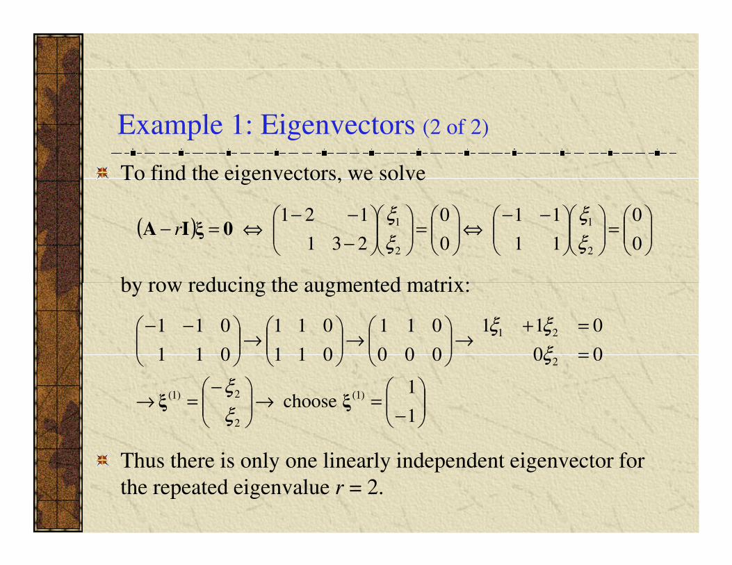
Example 1: Eigenvectors (2 of 2)
To find the eigenvectors, we solve
by row reducing the augmented matrix:
( )
=
−−⇔
=
−
−−⇔=−
0
0
11
11
0
0
231
121
2
1
2
1
ξ
ξ
ξ
ξ0ξIA r
by row reducing the augmented matrix:
Thus there is only one linearly independent eigenvector for
the repeated eigenvalue r = 2.
−=→
−=→
=
=+→
→
→
−−
1
1choose
00
011
000
011
011
011
011
011
)1(
2
2)1(
2
21
ξξξ
ξ
ξ
ξξ
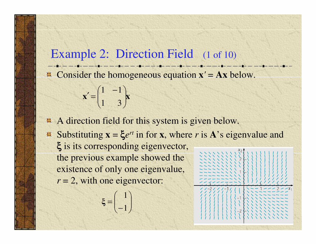
Example 2: Direction Field (1 of 10)
Consider the homogeneous equation x' = Ax below.
A direction field for this system is given below.
xx
−=′
31
11
A direction field for this system is given below.
Substituting x = ξξξξert in for x, where r is A’s eigenvalue and
ξξξξ is its corresponding eigenvector,
the previous example showed the
existence of only one eigenvalue,
r = 2, with one eigenvector:
−=
1
1ξ
Example 2: First Solution; and
Second Solution, First Attempt (2 of 10)
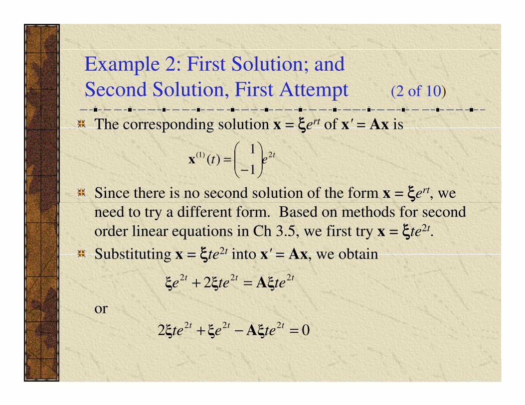
The corresponding solution x = ξξξξert of x' = Ax is
Since there is no second solution of the form x = ξξξξert, we
need to try a different form. Based on methods for second
tet
2)1(
1
1)(
−=x
need to try a different form. Based on methods for second
order linear equations in Ch 3.5, we first try x = ξξξξte2t.
Substituting x = ξξξξte2t into x' = Ax, we obtain
or
ttttetee
222 2 Aξξξ =+
02 222 =−+ tttteete Aξξξ
Example 2:
Second Solution, Second Attempt (3 of 10)
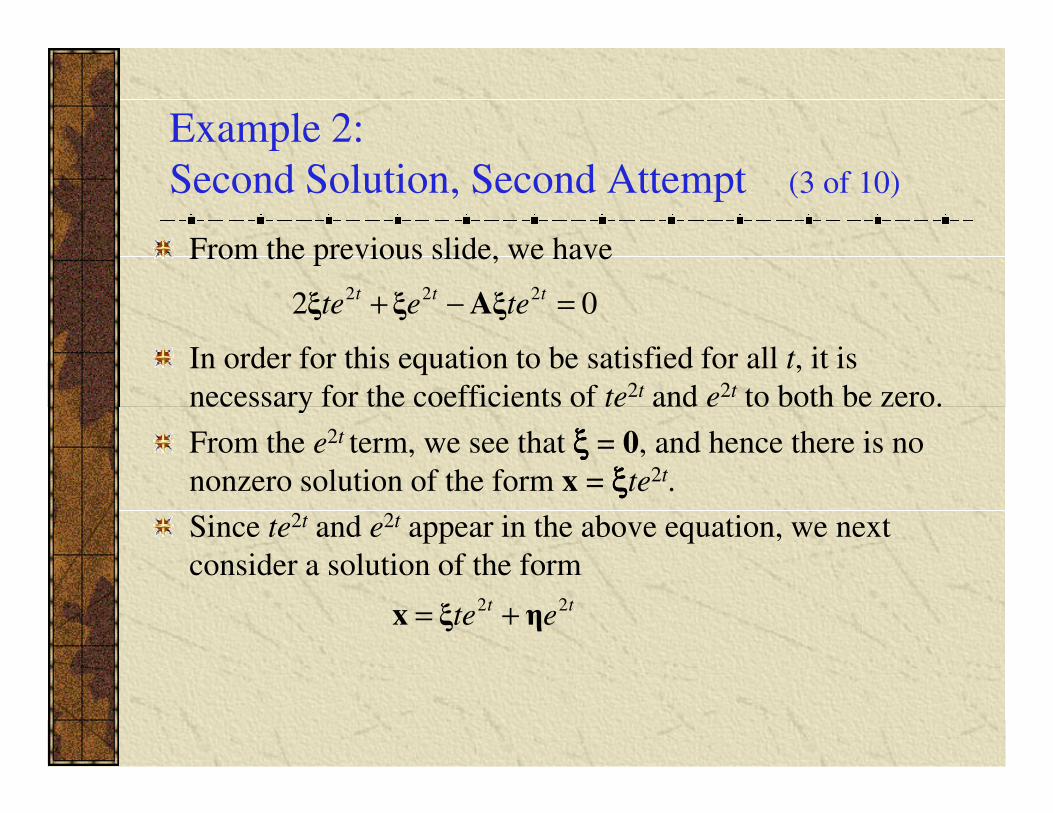
From the previous slide, we have
In order for this equation to be satisfied for all t, it is
necessary for the coefficients of te2t and e2t to both be zero.
02 222 =−+ tttteete Aξξξ
necessary for the coefficients of te and e to both be zero.
From the e2t term, we see that ξξξξ = 0, and hence there is no
nonzero solution of the form x = ξξξξte2t.
Since te2t and e2t appear in the above equation, we next
consider a solution of the form tt
ete22 ηξx +=
Example 2: Second Solution and its
Defining Matrix Equations (4 of 10)
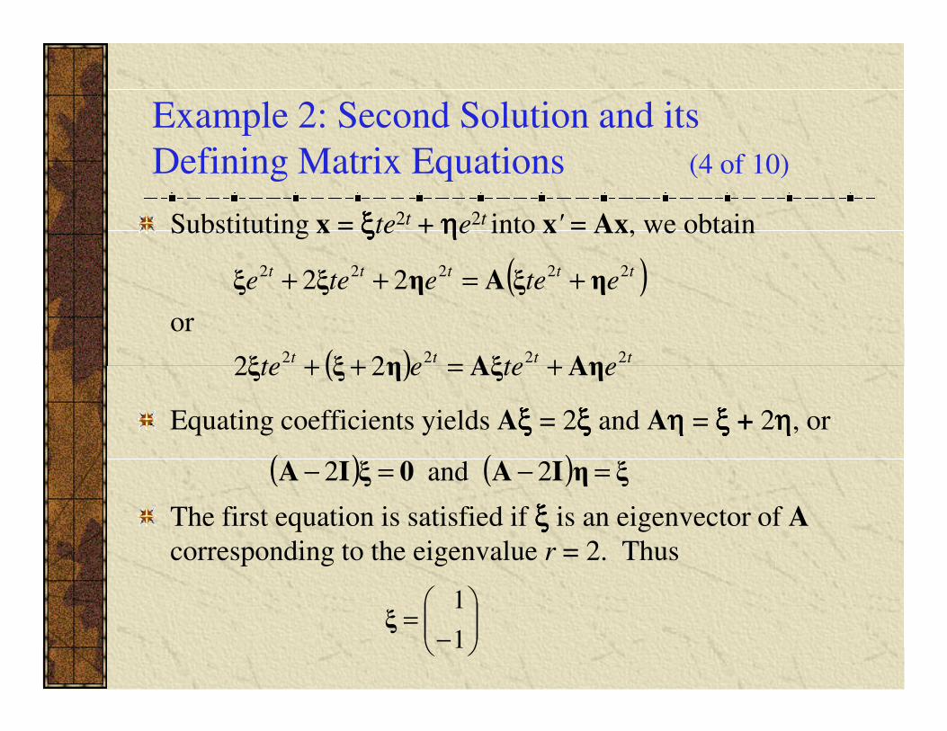
Substituting x = ξξξξte2t + ηηηηe2t into x' = Ax, we obtain
or
( )ttttteteetee
22222 22 ηξAηξξ +=++
( ) tttteteete
2222 22 AηAξηξξ +=++
Equating coefficients yields Aξξξξ = 2ξξξξ and Aηηηη = ξξξξ + 2ηηηη, or
The first equation is satisfied if ξξξξ is an eigenvector of A
corresponding to the eigenvalue r = 2. Thus
( ) tttteteete
2222 22 AηAξηξξ +=++
( ) ( ) ξηIA0ξIA =−=− 2and2
−=
1
1ξ
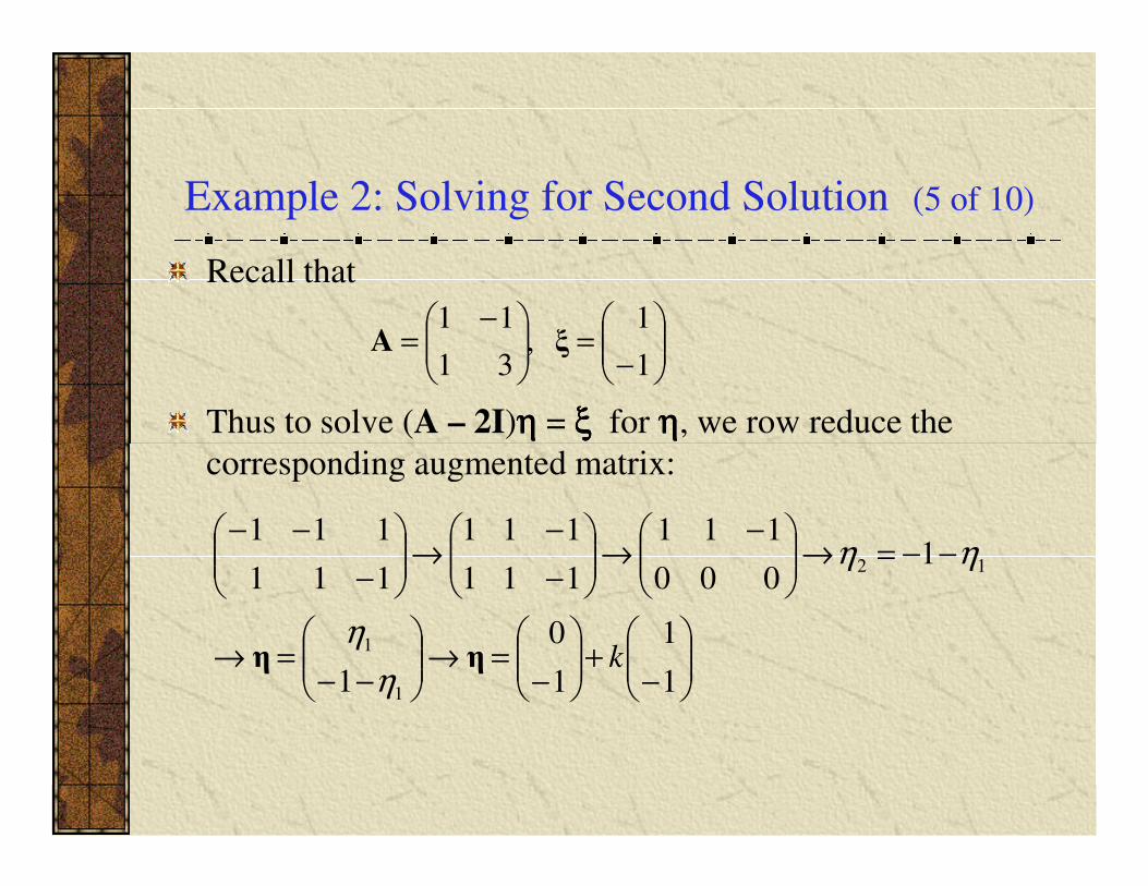
Example 2: Solving for Second Solution (5 of 10)
Recall that
Thus to solve (A – 2I)ηηηη = ξξξξ for ηηηη, we row reduce the
corresponding augmented matrix:
−=
−=
1
1,
31
11ξA
corresponding augmented matrix:
−+
−=→
−−=→
−−=→
−→
−
−→
−
−−
1
1
1
0
1
1000
111
111
111
111
111
1
1
12
kηηη
η
ηη

Example 2: Second Solution (6 of 10)
Our second solution x = ξξξξte2t + ηηηηe2t is now
Recalling that the first solution was
tttekete
222
1
1
1
0
1
1
−+
−+
−=x
we see that our second solution is simply
since the last term of third term of x is a multiple of x(1).
,1
1)( 2)1( t
et
−=x
,1
0
1
1)( 22)2( tt
etet
−+
−=x
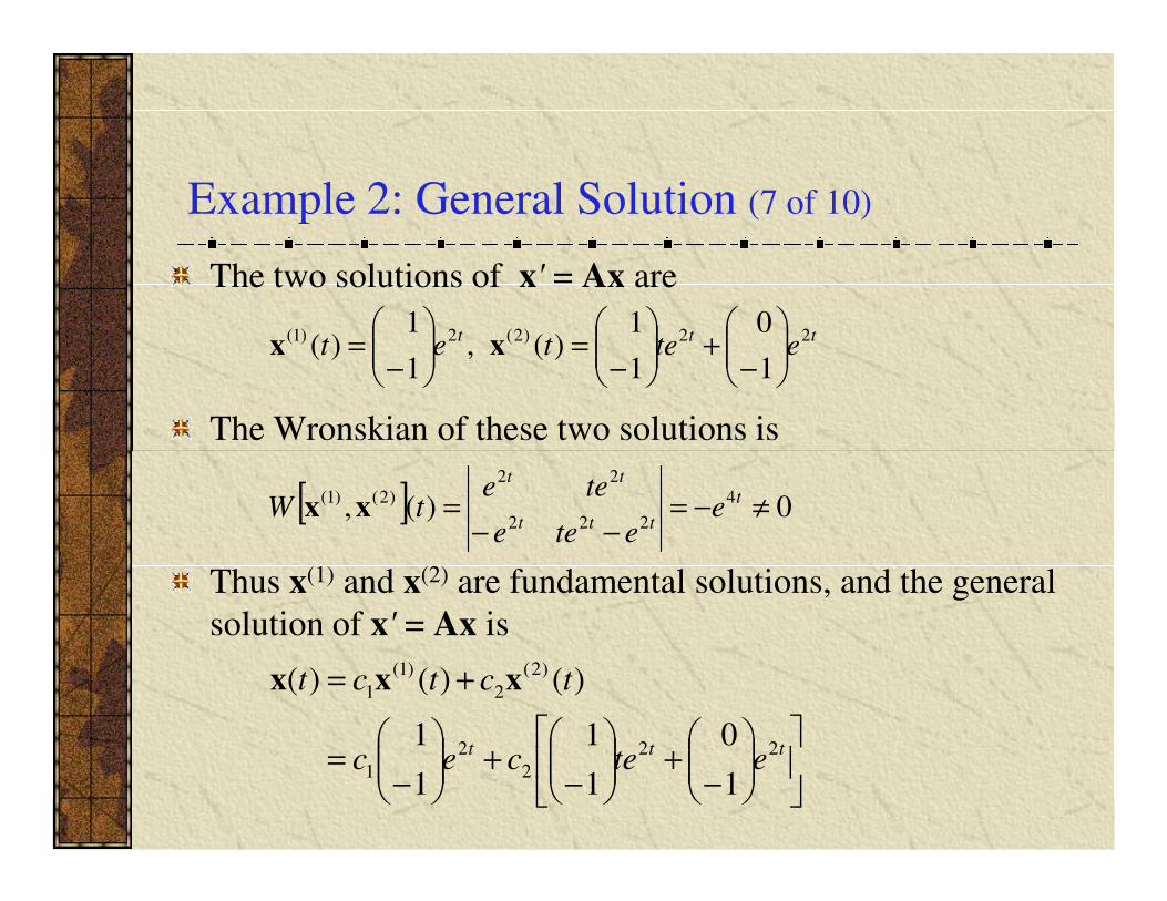
Example 2: General Solution (7 of 10)
The two solutions of x' = Ax are
The Wronskian of these two solutions is
tttetetet
22)2(2)1(
1
0
1
1)(,
1
1)(
−+
−=
−= xx
Thus x(1) and x(2) are fundamental solutions, and the general
solution of x' = Ax is
[ ] 0)(, 4
222
22
)2()1( ≠−=−−
= t
ttt
tt
eetee
teetW xx
−+
−+
−=
+=
tttetecec
tctct
22
2
2
1
)2(
2
)1(
1
1
0
1
1
1
1
)()()( xxx

Example 2: Phase Plane (8 of 10)
The general solution is
Thus x is unbounded as t → ∞, and x → 0 as t → -∞.
−+
−+
−= ttt
etecect22
2
2
11
0
1
1
1
1)(x
Further, it can be shown that as t → -∞, x → 0 asymptotic
to the line x2 = -x1 determined by the first eigenvector.
Similarly, as t → ∞, x is asymptotic
to a line parallel to x2 = -x1.
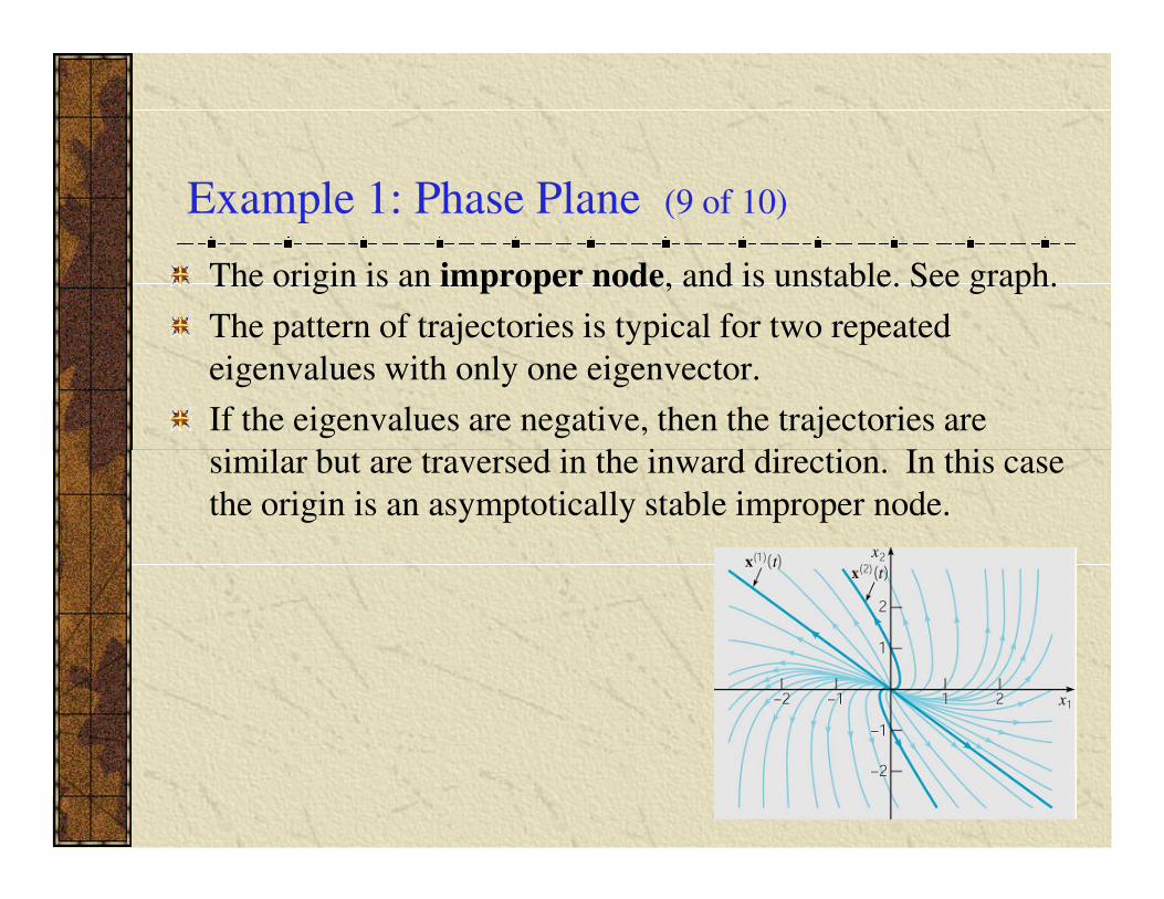
Example 1: Phase Plane (9 of 10)
The origin is an improper node, and is unstable. See graph.
The pattern of trajectories is typical for two repeated
eigenvalues with only one eigenvector.
If the eigenvalues are negative, then the trajectories are
similar but are traversed in the inward direction. In this case similar but are traversed in the inward direction. In this case
the origin is an asymptotically stable improper node.
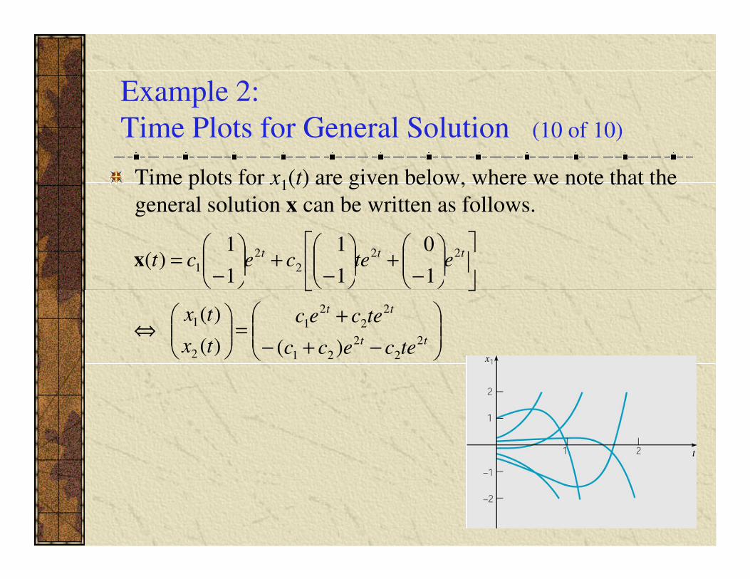
Example 2:
Time Plots for General Solution (10 of 10)
Time plots for x1(t) are given below, where we note that the
general solution x can be written as follows.
−+
−+
−= ttt
etecect22
2
2
11
0
1
1
1
1)(x
−+−
+=
⇔
tt
tt
tececc
tecec
tx
tx
2
2
2
21
2
2
2
1
2
1
)()(
)(
General Case for Double Eigenvalues
Suppose the system x' = Ax has a double eigenvalue r = ρand a single corresponding eigenvector ξξξξ.
The first solution is
x(1) = ξξξξeρ t,
where ξξξξ satisfies (A-ρI)ξξξξ = 0. where ξξξξ satisfies (A-ρI)ξξξξ = 0.
As in Example 1, the second solution has the form
where ξξξξ is as above and ηηηη satisfies (A-ρI)ηηηη = ξξξξ.
Since ρ is an eigenvalue, det(A-ρI) = 0, and (A-ρI)ηηηη = bdoes not have a solution for all b. However, it can be shown that (A-ρI)ηηηη = ξξξξ always has a solution.
The vector ηηηη is called a generalized eigenvector.
ttete
ρρ ηξx +=)2(
Example 2 Extension:
Fundamental Matrix ΨΨΨΨ (1 of 2)
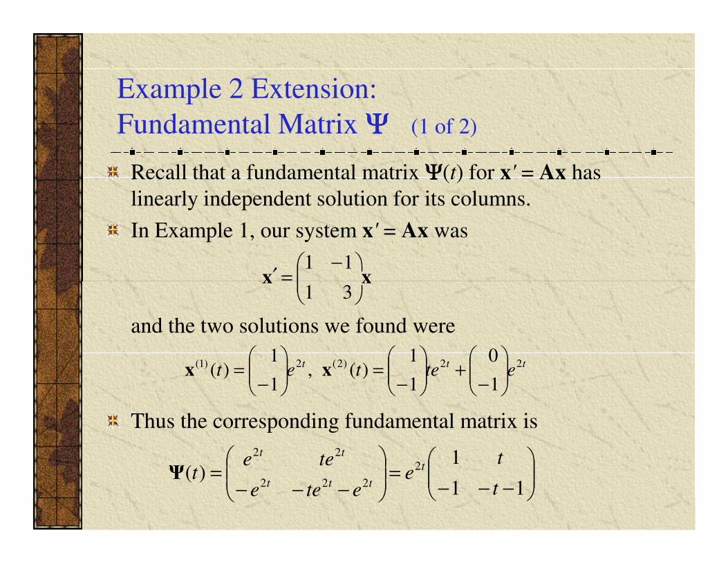
Recall that a fundamental matrix ΨΨΨΨ(t) for x' = Ax has
linearly independent solution for its columns.
In Example 1, our system x' = Ax was
xx
−
=′31
11
and the two solutions we found were
Thus the corresponding fundamental matrix is
−−−=
−−−=
11
1)( 2
222
22
t
te
etee
teet
t
ttt
tt
Ψ
tttetetet
22)2(2)1(
1
0
1
1)(,
1
1)(
−+
−=
−= xx
xx
=′31
Example 2 Extension:
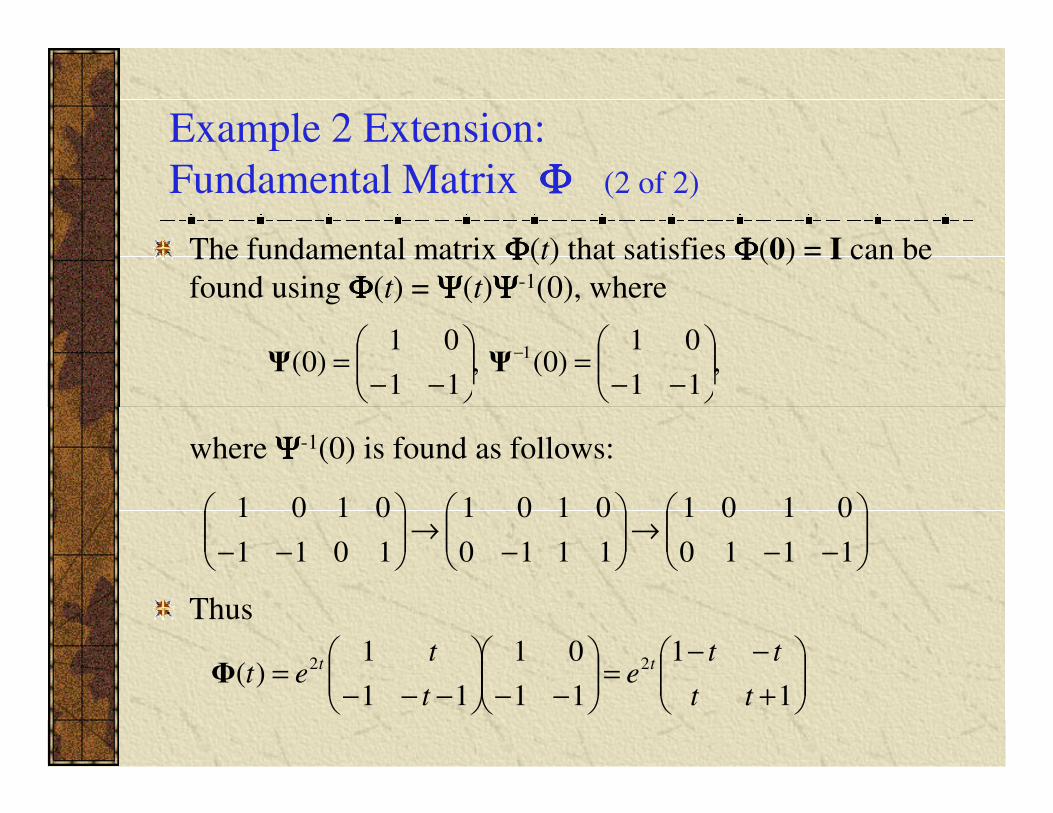
Fundamental Matrix ΦΦΦΦ (2 of 2)
The fundamental matrix ΦΦΦΦ(t) that satisfies ΦΦΦΦ(0) = I can be
found using ΦΦΦΦ(t) = ΨΨΨΨ(t)ΨΨΨΨ-1(0), where
,11
01)0(,
11
01)0( 1
−−=
−−= −
ΨΨ
where ΨΨΨΨ-1(0) is found as follows:
Thus
−−→
−→
−− 1110
0101
1110
0101
1011
0101
+
−−=
−−
−−−=
1
1
11
01
11
1)( 22
tt
tte
t
tet
ttΦ

Jordan Forms
If A is n x n with n linearly independent eigenvectors, then A
can be diagonalized using a similarity transform T-1AT = D.The transform matrix T consisted of eigenvectors of A, and
the diagonal entries of D consisted of the eigenvalues of A.
In the case of repeated eigenvalues and fewer than n linearly In the case of repeated eigenvalues and fewer than n linearly
independent eigenvectors, A can be transformed into a nearly
diagonal matrix J, called the Jordan form of A, with
T-1AT = J.
Example 2 Extension:
Transform Matrix (1 of 2)
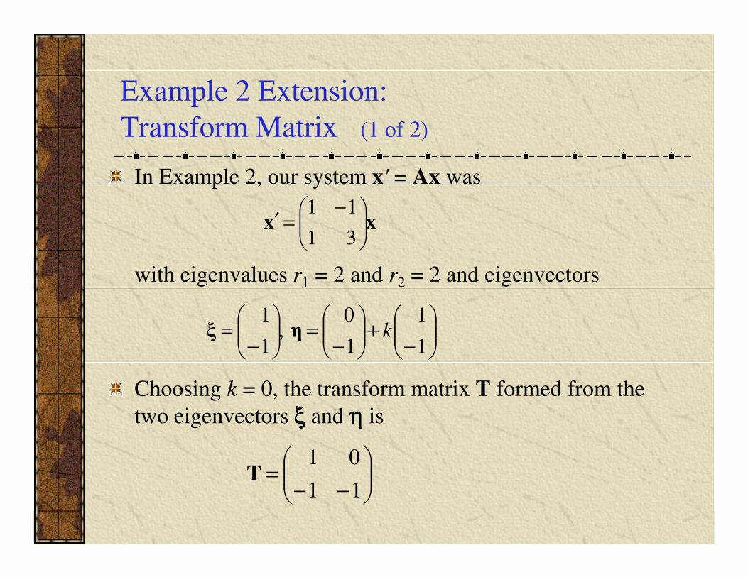
In Example 2, our system x' = Ax was
with eigenvalues r1 = 2 and r2 = 2 and eigenvectors
xx
−=′
31
11
1 2
Choosing k = 0, the transform matrix T formed from the
two eigenvectors ξξξξ and ηηηη is
−+
−=
−=
1
1
1
0,
1
1kηξ
−−=
11
01T
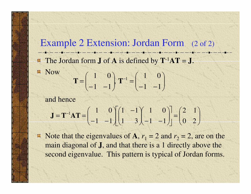
Example 2 Extension: Jordan Form (2 of 2)
The Jordan form J of A is defined by T-1AT = J.
Now
and hence
−−=
−−= −
11
01,
11
011TT
and hence
Note that the eigenvalues of A, r1 = 2 and r2 = 2, are on the
main diagonal of J, and that there is a 1 directly above the
second eigenvalue. This pattern is typical of Jordan forms.
=
−−
−
−−== −
20
12
11
01
31
11
11
011ATTJ


![INTRODUC¸AO˜ AS EQUAC¸` OES DIFERENCIAIS ORDIN˜ …satuf.net/2017_2/MAI/livro1.pdf · Este ´e um texto alternativo ao excelente livro Boyce-DiPrima [ 1] para a parte de equac¸oes](https://static.fdocuments.in/doc/165x107/5bea9b7f09d3f28d5d8bad2b/introducao-as-equac-oes-diferenciais-ordin-satufnet20172mai-este.jpg)

![[William E. Boyce, Richard C. DiPrima] Elementary (BookZZ.org)](https://static.fdocuments.in/doc/165x107/55cf9326550346f57b9c2ea7/william-e-boyce-richard-c-diprima-elementary-bookzzorg.jpg)