Boyce/DiPrima/Meade 11th ed, Ch 4.1: Higher

Order Linear ODEs: General Theory

Elementary Differential Equations and Boundary Value Problems, 11th edition, by William E. Boyce, Richard C. DiPrima, and Doug Meade ©2017 by John

Wiley & Sons, Inc.

• An nth order ODE has the general form

• We assume that P0,…, Pn, and G are continuous real-valued

functions on some interval , and that P0 is nowhere

zero on I.

• Dividing by P0, the ODE becomes

• For an nth order ODE, there are typically n initial conditions:

tGytPdt

dytP

dt

ydtP

dt

ydtP nnn

n

n

n

)()()()( 11

1

10

tgytpdt

dytp

dt

ydtp

dt

ydyL nnn

n

n

n

)()()( 11

1

1

)1(

00

)1(

0000 ,,, nn ytyytyyty

I = (a,b)

Theorem 4.1.1

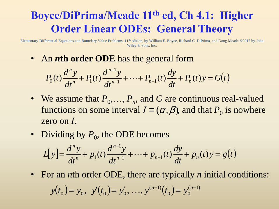
• Consider the nth order initial value problem

• If the functions p1,…, pn, and g are continuous on an open

interval I, then there exists exactly one solution

that satisfies the initial value problem. This solution exists

throughout the interval I.

)1(

00

)1(

0000

11

1

1

,,,

)()()(

nn

nnn

n

n

n

ytyytyyty

tgytpdt

dytp

dt

ydtp

dt

yd

y = f(t)

Homogeneous Equations

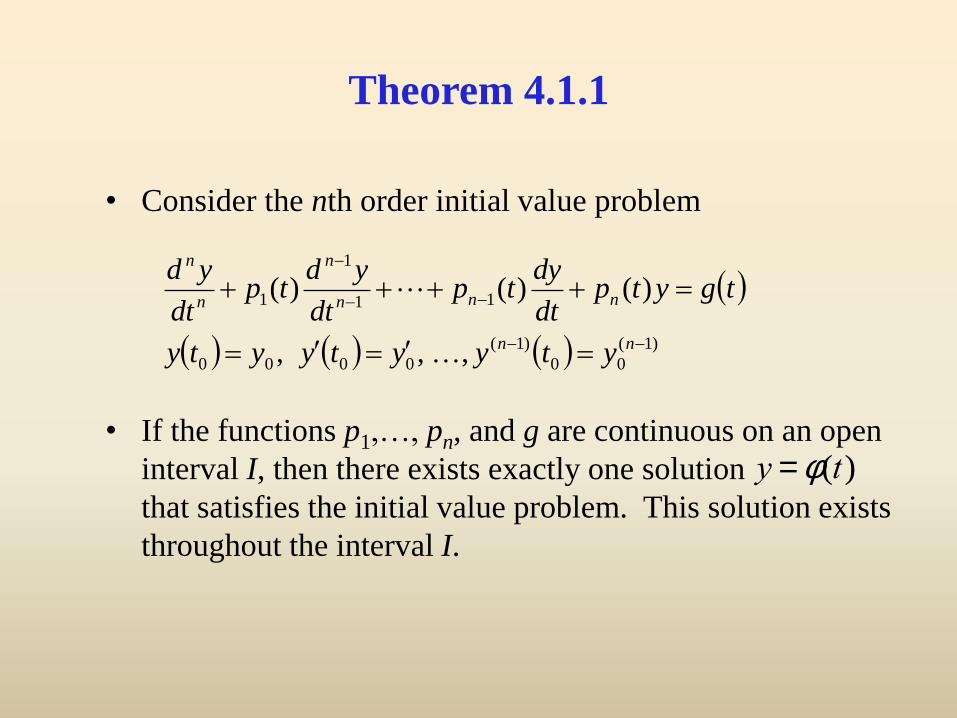
• As with 2nd order case, we begin with homogeneous ODE:

• If y1,…, yn are solns to ODE, then so is linear combination

• Every soln can be expressed in this form, with coefficients

determined by initial conditions, iff we can solve:

0)()()( 11

1

1

ytpdt

dytp

dt

ydtp

dt

ydyL nnn

n

n

n

)()()()( 2211 tyctyctycty nn

)1(

00

)1(

0

)1(

11

00011

00011

)()(

)()(

)()(

nn

nn

n

nn

nn

ytyctyc

ytyctyc

ytyctyc

Homogeneous Equations & Wronskian

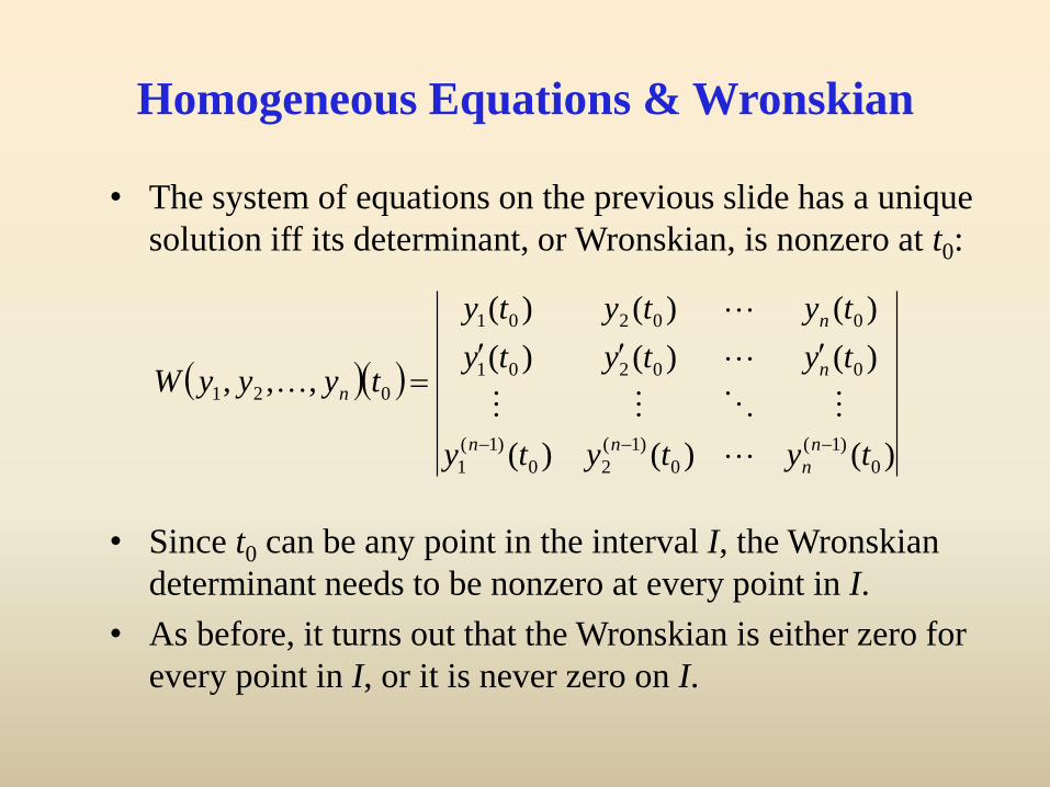
• The system of equations on the previous slide has a unique

solution iff its determinant, or Wronskian, is nonzero at t0:

• Since t0 can be any point in the interval I, the Wronskian

determinant needs to be nonzero at every point in I.

• As before, it turns out that the Wronskian is either zero for

every point in I, or it is never zero on I.

)()()(

)()()(

)()()(

,,,

0

)1(

0

)1(

20

)1(

1

00201

00201

021

tytyty

tytyty

tytyty

tyyyW

n

n

nn

n

n

n

Theorem 4.1.2

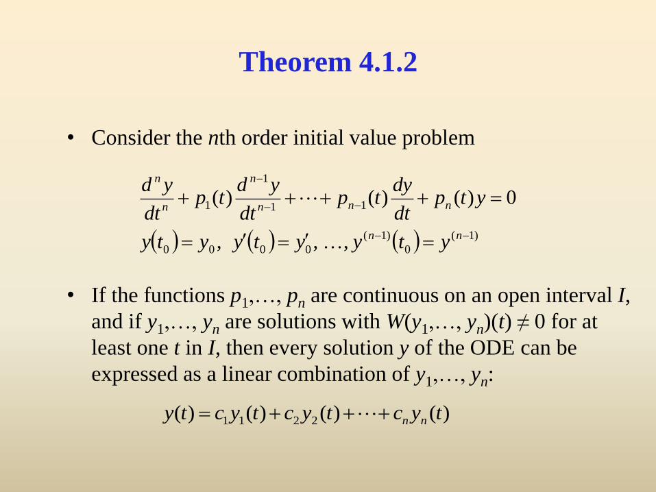
• Consider the nth order initial value problem

• If the functions p1,…, pn are continuous on an open interval I,

and if y1,…, yn are solutions with W(y1,…, yn)(t) ≠ 0 for at

least one t in I, then every solution y of the ODE can be

expressed as a linear combination of y1,…, yn:

)1(

0

)1(

0000

11

1

1

,,,

0)()()(

nn

nnn

n

n

n

ytyytyyty

ytpdt

dytp

dt

ydtp

dt

yd

)()()()( 2211 tyctyctycty nn

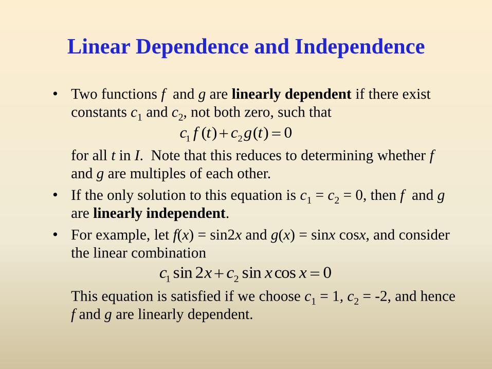
Linear Dependence and Independence

• Two functions f and g are linearly dependent if there exist

constants c1 and c2, not both zero, such that

for all t in I. Note that this reduces to determining whether f

and g are multiples of each other.

• If the only solution to this equation is c1 = c2 = 0, then f and g

are linearly independent.

• For example, let f(x) = sin2x and g(x) = sinx cosx, and consider

the linear combination

This equation is satisfied if we choose c1 = 1, c2 = -2, and hence

f and g are linearly dependent.

0)()( 21 tgctfc

0cossin2sin 21 xxcxc

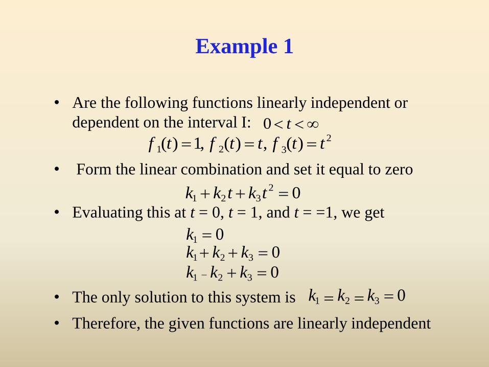
Example 1

• Are the following functions linearly independent or

dependent on the interval I:

• Form the linear combination and set it equal to zero

• Evaluating this at t = 0, t = 1, and t = =1, we get

• The only solution to this system is

• Therefore, the given functions are linearly independent

2

321 )(,)(,1)( ttfttftf

t0

02321 tktkk

0

00

321

321

1

kkk

kkkk

0321 kkk

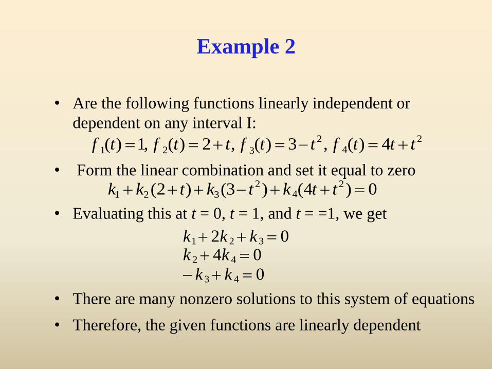
Example 2

• Are the following functions linearly independent or

dependent on any interval I:

• Form the linear combination and set it equal to zero

• Evaluating this at t = 0, t = 1, and t = =1, we get

• There are many nonzero solutions to this system of equations

• Therefore, the given functions are linearly dependent

24

2

321 4)(,3)(,2)(,1)( tttfttfttftf

0)4()3()2( 24

2321 ttktktkk

0

0402

43

42

321

kk

kkkkk

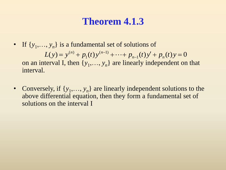
Theorem 4.1.3

• If {y1,…, yn} is a fundamental set of solutions of

on an interval I, then {y1,…, yn} are linearly independent on that interval.

• Conversely, if {y1,…, yn} are linearly independent solutions to the above differential equation, then they form a fundamental set of solutions on the interval I

0)()()()( 1

)1(

1

)(

ytpytpytpyyL nn

nn

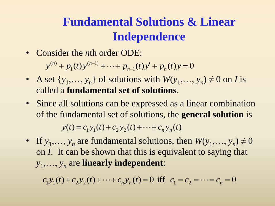
Fundamental Solutions & Linear

Independence

• Consider the nth order ODE:

• A set {y1,…, yn} of solutions with W(y1,…, yn) ≠ 0 on I is

called a fundamental set of solutions.

• Since all solutions can be expressed as a linear combination

of the fundamental set of solutions, the general solution is

• If y1,…, yn are fundamental solutions, then W(y1,…, yn) ≠ 0

on I. It can be shown that this is equivalent to saying that

y1,…, yn are linearly independent:

0)()()( 1

)1(

1

)(

ytpytpytpy nn

nn

)()()()( 2211 tyctyctycty nn

0 iff 0)()()( 212211 nnn ccctyctyctyc

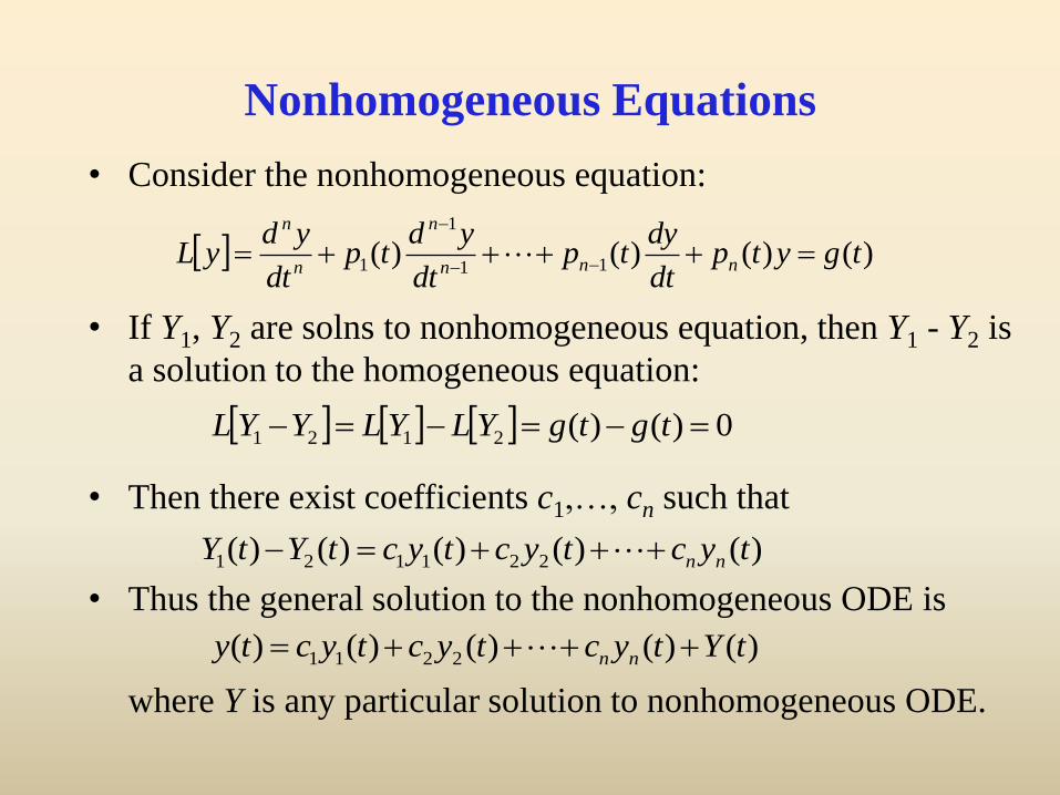
Nonhomogeneous Equations

• Consider the nonhomogeneous equation:

• If Y1, Y2 are solns to nonhomogeneous equation, then Y1 - Y2 is

a solution to the homogeneous equation:

• Then there exist coefficients c1,…, cn such that

• Thus the general solution to the nonhomogeneous ODE is

where Y is any particular solution to nonhomogeneous ODE.

)()()()( 11

1

1 tgytpdt

dytp

dt

ydtp

dt

ydyL nnn

n

n

n

0)()(2121 tgtgYLYLYYL

)()()()()( 221121 tyctyctyctYtY nn

)()()()()( 2211 tYtyctyctycty nn

Boyce/DiPrima/Meade 11th ed, Ch 4.2: Homogeneous

Differential Equations with Constant Coefficients

Elementary Differential Equations and Boundary Value Problems, 11th edition, by William E. Boyce, Richard C. DiPrima, and Doug Meade ©2017 by John

Wiley & Sons, Inc.

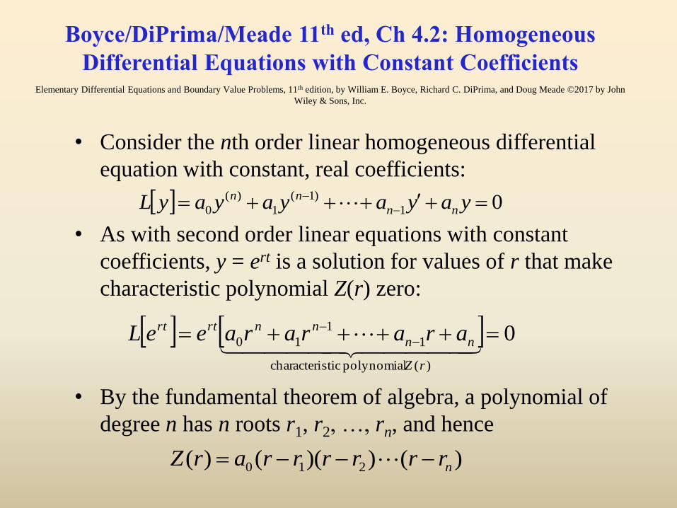
• Consider the nth order linear homogeneous differential

equation with constant, real coefficients:

• As with second order linear equations with constant

coefficients, y = ert is a solution for values of r that make

characteristic polynomial Z(r) zero:

• By the fundamental theorem of algebra, a polynomial of

degree n has n roots r1, r2, …, rn, and hence

01

)1(

1

)(

0

yayayayayL nn

nn

0

)( polynomial sticcharacteri

1

1

10

rZ

nn

nnrtrt arararaeeL

)())(()( 210 nrrrrrrarZ

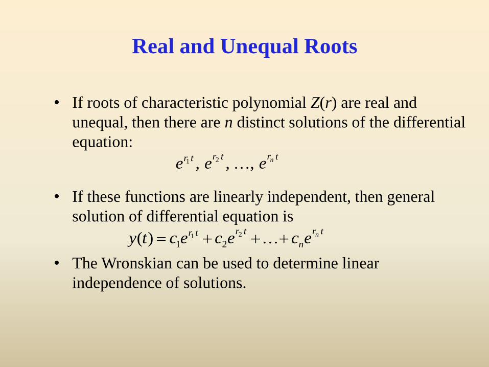
Real and Unequal Roots

• If roots of characteristic polynomial Z(r) are real and

unequal, then there are n distinct solutions of the differential

equation:

• If these functions are linearly independent, then general

solution of differential equation is

• The Wronskian can be used to determine linear

independence of solutions.

trtrtr neee ,,, 21

tr

n

trtr necececty 21

21)(

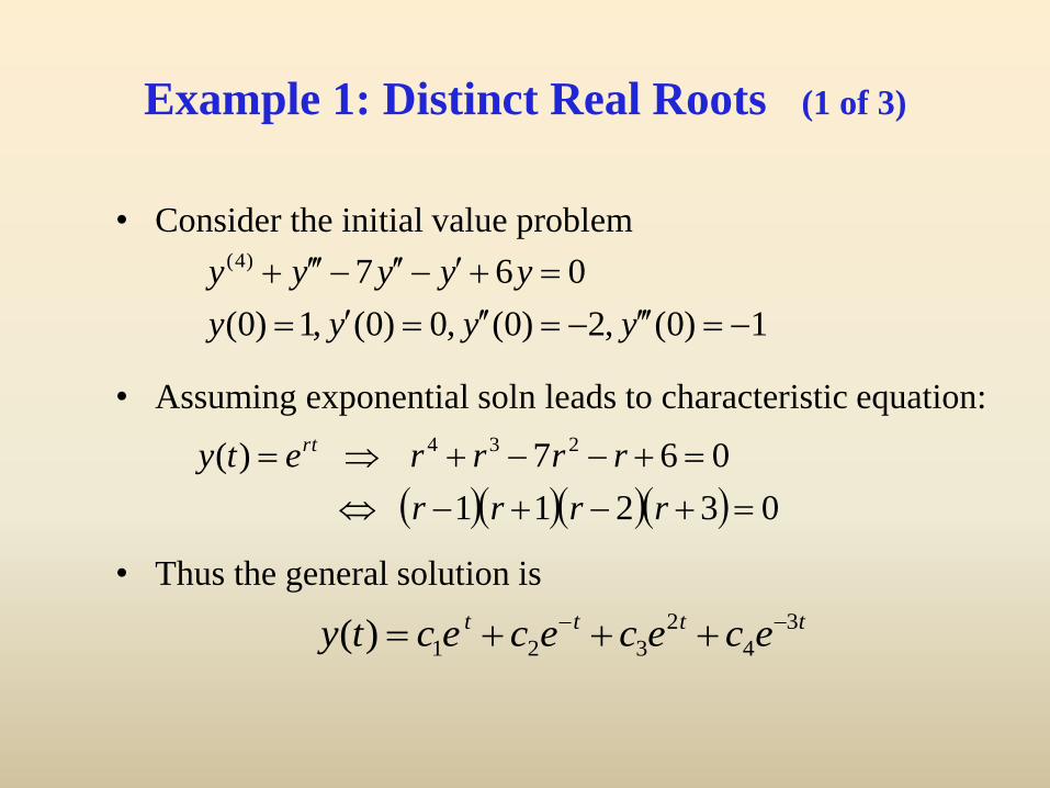
Example 1: Distinct Real Roots (1 of 3)

• Consider the initial value problem

• Assuming exponential soln leads to characteristic equation:

• Thus the general solution is

03211

067)( 234

rrrr

rrrrety rt

tttt ececececty 3

4

2

321)(

1)0(,2)0(,0)0(,1)0(

067)4(

yyyy

yyyyy

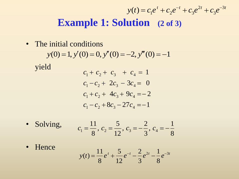
Example 1: Solution (2 of 3)

• The initial conditions

yield

• Solving,

• Hence

1278

294

032

1

4321

4321

4321

4321

cccc

cccc

cccc

cccc

1)0(,2)0(,0)0(,1)0( yyyy

tttt ececececty 3

3

2

321)(

8

1,

3

2,

12

5,

8

114321 cccc

tttt eeeety 32

8

1

3

2

12

5

8

11)(

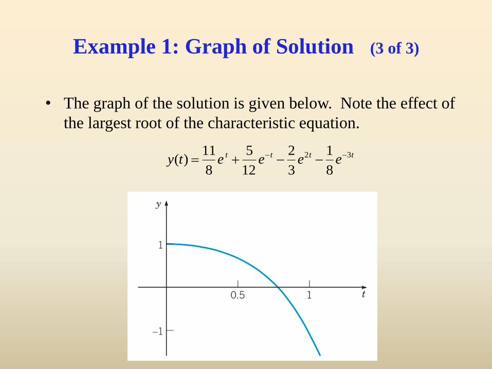
Example 1: Graph of Solution (3 of 3)

• The graph of the solution is given below. Note the effect of

the largest root of the characteristic equation.

tttt eeeety 32

8

1

3

2

12

5

8

11)(

Complex Roots

• If the characteristic polynomial Z(r) has complex roots, then

they must occur in conjugate pairs, .

• Note that not all the roots need be complex.

• Solutions corresponding to complex roots have the form

• As in Chapter 3.4, we use the real-valued solutions

tietee

tietee

ttti

ttti

sincos

sincos

tete tt sin,cos

l ± im

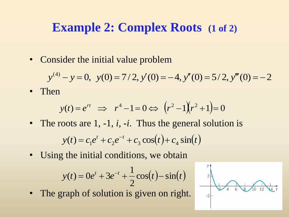
Example 2: Complex Roots (1 of 2)

• Consider the initial value problem

• Then

• The roots are 1, -1, i, -i. Thus the general solution is

• Using the initial conditions, we obtain

• The graph of solution is given on right.

01101)( 224 rrrety rt

2)0(,2/5)0(,4)0(,2/7)0(,0)4( yyyyyy

tctcececty tt sincos)( 4321

tteety tt sincos2

130)(

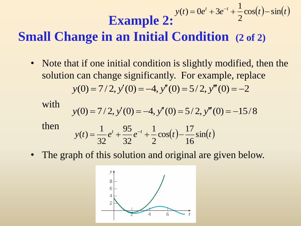
Example 2:

Small Change in an Initial Condition (2 of 2)

• Note that if one initial condition is slightly modified, then the

solution can change significantly. For example, replace

with

then

• The graph of this solution and original are given below.

tteety tt sincos2

130)(

2)0(,2/5)0(,4)0(,2/7)0( yyyy

8/15)0(,2/5)0(,4)0(,2/7)0( yyyy

tteety tt sin16

17cos

2

1

32

95

32

1)(

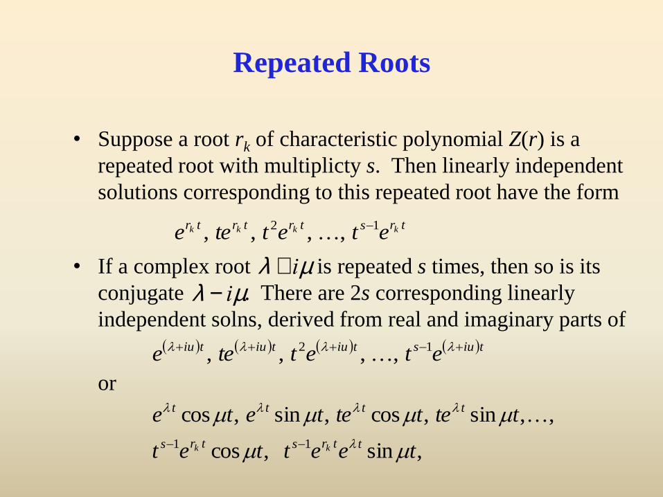
Repeated Roots

• Suppose a root rk of characteristic polynomial Z(r) is a

repeated root with multiplicty s. Then linearly independent

solutions corresponding to this repeated root have the form

• If a complex root is repeated s times, then so is its

conjugate . There are 2s corresponding linearly

independent solns, derived from real and imaginary parts of

or

trstrtrtr kkkk etettee 12 ,,,,

,sin,cos

,,sin,cos,sin,cos

11 teettet

ttettetete

ttrstrs

tttt

kk

tiustiutiutiu etettee 12 ,,,,

l + iml - im

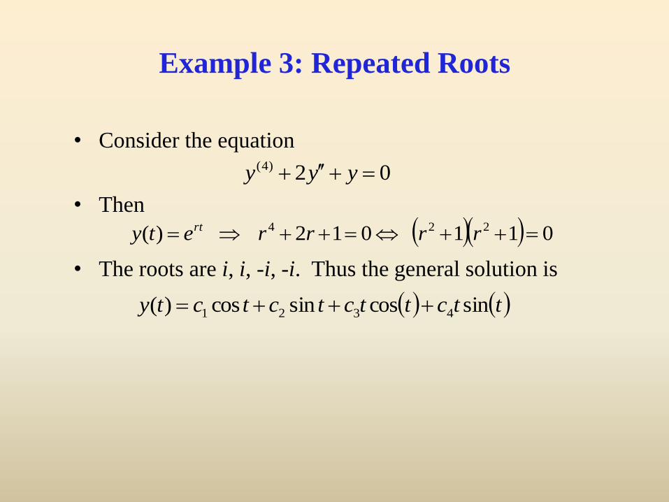
Example 3: Repeated Roots

• Consider the equation

• Then

• The roots are i, i, -i, -i. Thus the general solution is

011012)( 224 rrrrety rt

02)4( yyy

ttcttctctcty sincossincos)( 4321

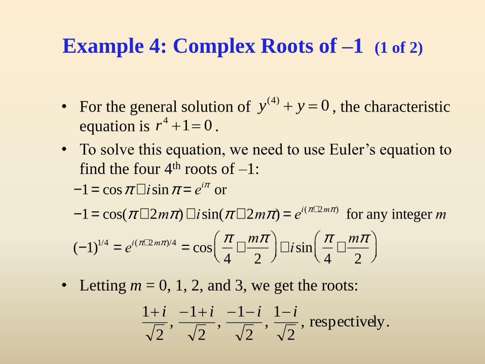
Example 4: Complex Roots of –1 (1 of 2)

• For the general solution of , the characteristic

equation is .

• To solve this equation, we need to use Euler’s equation to

find the four 4th roots of –1:

• Letting m = 0, 1, 2, and 3, we get the roots:

014 r

0)4( yy

-1 = cosp + isinp = eip or

-1 = cos(p + 2mp )+ isin(p + 2mp ) = ei(p+2mp ) for any integer m

(-1)1/4 = ei(p+2mp )/4 = cosp

4+mp

2

æ

èçö

ø÷+ isin

p

4+mp

2

æ

èçö

ø÷

ly.respective,2

1,

2

1,

2

1,

2

1 iiii

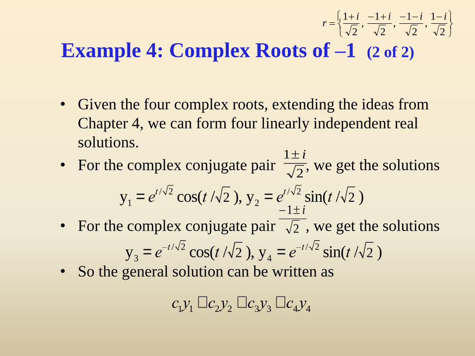
Example 4: Complex Roots of –1 (2 of 2)

• Given the four complex roots, extending the ideas from

Chapter 4, we can form four linearly independent real

solutions.

• For the complex conjugate pair , we get the solutions

• For the complex conjugate pair , we get the solutions

• So the general solution can be written as

2

1,

2

1,

2

1,

2

1 iiiir

2

1 i

y1 = et / 2 cos(t / 2 ), y2 = et / 2 sin(t / 2 )

2

1 i

y3 = e–t / 2 cos(t / 2 ), y4 = e–t / 2 sin(t / 2 )

c1y1 + c2y2 + c3y3 + c4y4

Boyce/DiPrima/Meade 11th ed, Ch 4.3: The Method of Undetermined

Coefficients

Elementary Differential Equations and Boundary Value Problems, 11th edition, by William E. Boyce, Richard C. DiPrima, and Doug Meade ©2017 by John Wiley & Sons, Inc.

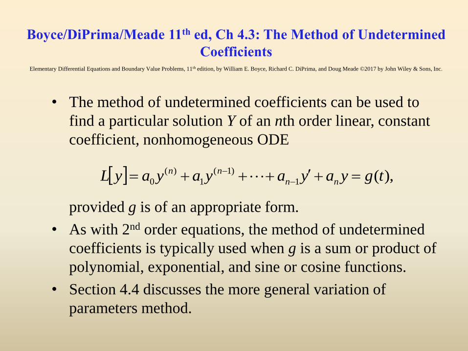
• The method of undetermined coefficients can be used to

find a particular solution Y of an nth order linear, constant

coefficient, nonhomogeneous ODE

provided g is of an appropriate form.

• As with 2nd order equations, the method of undetermined

coefficients is typically used when g is a sum or product of

polynomial, exponential, and sine or cosine functions.

• Section 4.4 discusses the more general variation of

parameters method.

),(1

)1(

1

)(

0 tgyayayayayL nn

nn

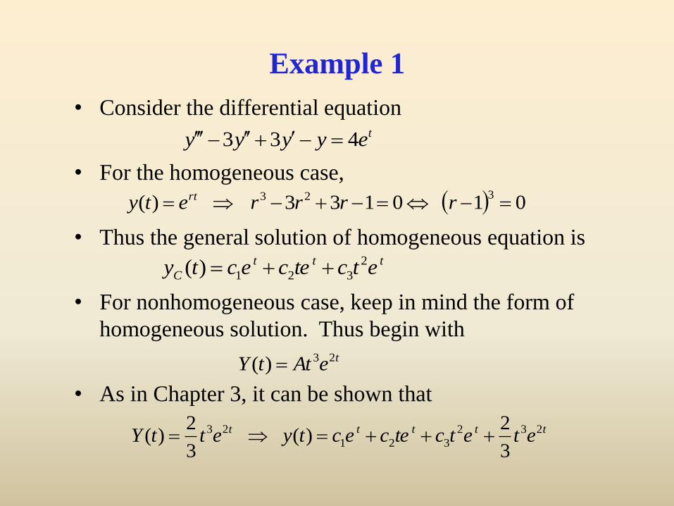
Example 1

• Consider the differential equation

• For the homogeneous case,

• Thus the general solution of homogeneous equation is

• For nonhomogeneous case, keep in mind the form of

homogeneous solution. Thus begin with

• As in Chapter 3, it can be shown that

teyyyy 433

teAttY 23)(

010133)(323 rrrrety rt

ttt

C etctececty 2

321)(

ttttt etetctecectyettY 232

321

23

3

2)(

3

2)(

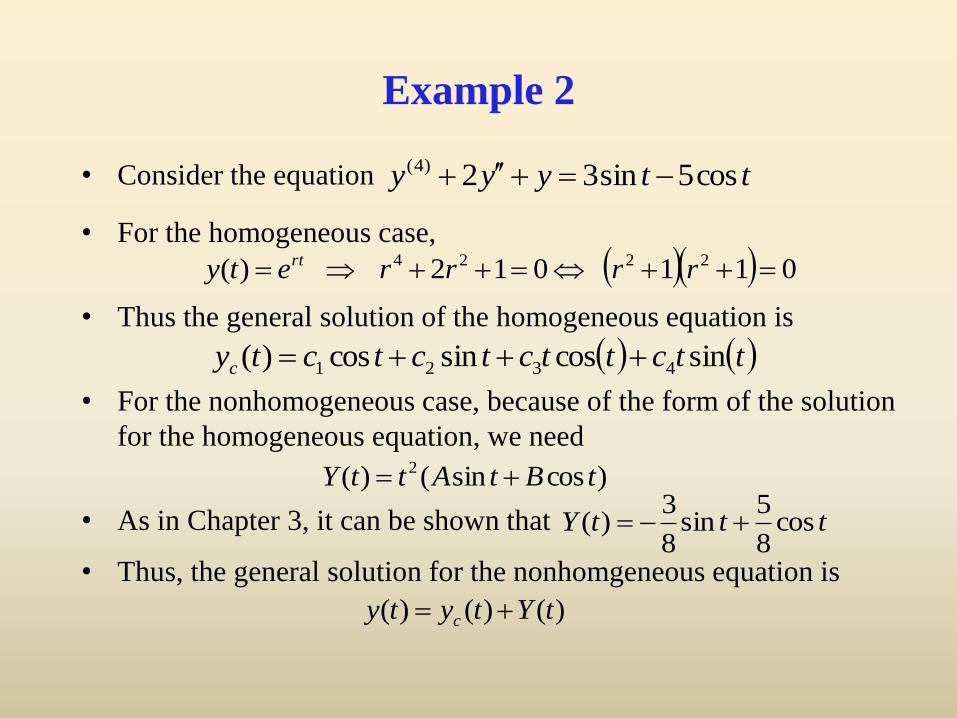
Example 2

• Consider the equation

• For the homogeneous case,

• Thus the general solution of the homogeneous equation is

• For the nonhomogeneous case, because of the form of the solution

for the homogeneous equation, we need

• As in Chapter 3, it can be shown that

• Thus, the general solution for the nonhomgeneous equation is

)cossin()( 2 tBtAttY

tttY cos8

5sin

8

3)(

ttyyy cos5sin32)4(

011012)( 2224 rrrrety rt

ttcttctctctyc sincossincos)( 4321

)()()( tYtyty c

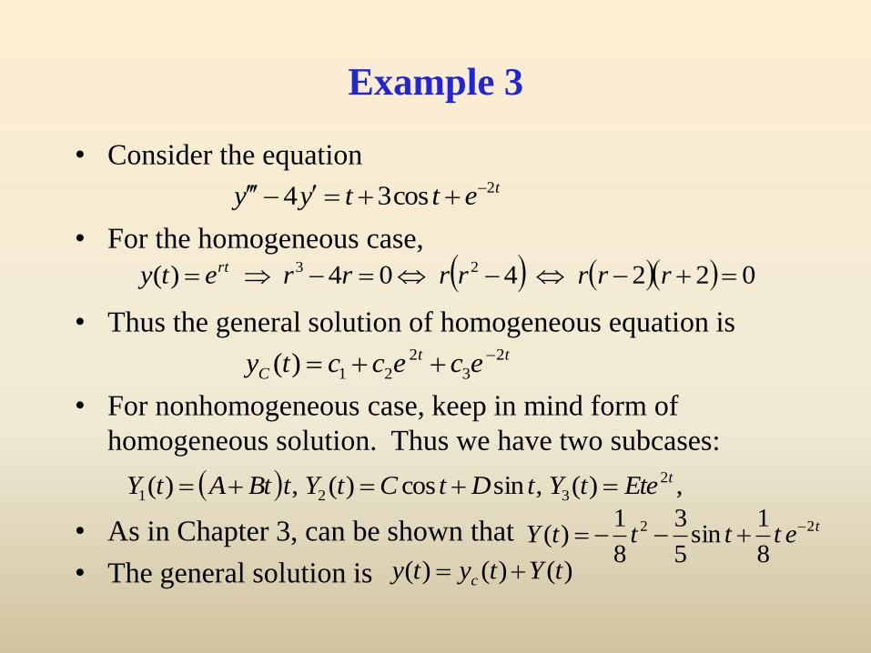
Example 3

• Consider the equation

• For the homogeneous case,

• Thus the general solution of homogeneous equation is

• For nonhomogeneous case, keep in mind form of

homogeneous solution. Thus we have two subcases:

• As in Chapter 3, can be shown that

• The general solution is

tettyy 2cos34

,)(,sincos)(,)( 2

321

tEtetYtDtCtYtBtAtY

022404)( 23 rrrrrrrety rt

tt

C ececcty 2

3

2

21)(

tettttY 22

8

1sin

5

3

8

1)(

)()()( tYtyty c

Boyce/DiPrima/Meade 11th ed, Ch 4.4:

The Method of Variation of Parameters

Elementary Differential Equations and Boundary Value Problems, 11th edition, by William E. Boyce, Richard C. DiPrima, and Doug Meade ©2017 by John Wiley

& Sons, Inc.

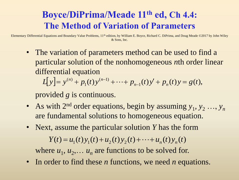
• The variation of parameters method can be used to find a

particular solution of the nonhomogeneous nth order linear

differential equation

provided g is continuous.

• As with 2nd order equations, begin by assuming y1, y2 …, yn

are fundamental solutions to homogeneous equation.

• Next, assume the particular solution Y has the form

where u1, u2,… un are functions to be solved for.

• In order to find these n functions, we need n equations.

),()()()( 1

)1(

1

)( tgytpytpytpyyL nn

nn

)()()()()()()( 2211 tytutytutytutY nn

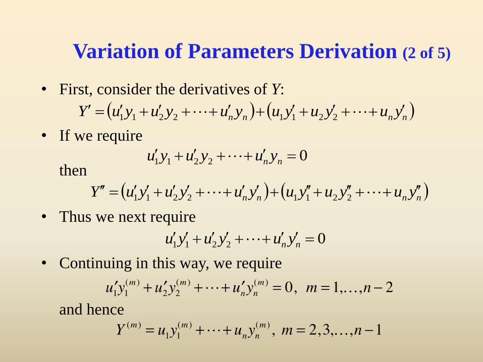
Variation of Parameters Derivation (2 of 5)

• First, consider the derivatives of Y:

• If we require

then

• Thus we next require

• Continuing in this way, we require

and hence

nnnn yuyuyuyuyuyuY 22112211

02211 nn yuyuyu

nnnn yuyuyuyuyuyuY 22112211

02211 nn yuyuyu

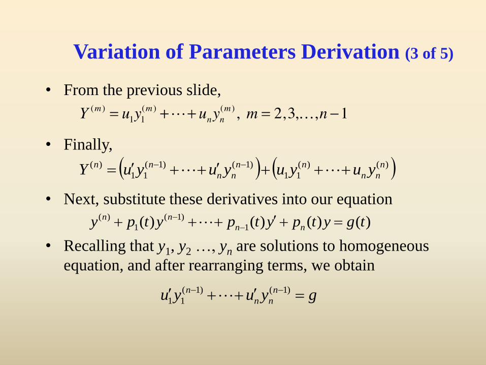
Variation of Parameters Derivation (3 of 5)

• From the previous slide,

• Finally,

• Next, substitute these derivatives into our equation

• Recalling that y1, y2 …, yn are solutions to homogeneous

equation, and after rearranging terms, we obtain

)()(

11

)1()1(

11

)( n

nn

nn

nn

nn yuyuyuyuY

gyuyu n

nn

n )1()1(

11

)()()()( 1

)1(

1

)( tgytpytpytpy nn

nn

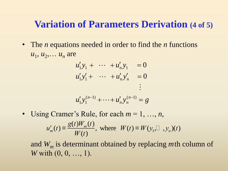
Variation of Parameters Derivation (4 of 5)

• The n equations needed in order to find the n functions

u1, u2,… un are

• Using Cramer’s Rule, for each m = 1, …, n,

and Wm is determinant obtained by replacing m th column of

W with (0, 0, …, 1).

gyuyu

yuyu

yuyu

n

nn

n

nn

n

)1()1(

11

11

111

0

0

¢um(t) =

g(t)Wm(t)

W (t), where W (t) =W (y1,… ,yn )(t)

Variation of Parameters Derivation (5 of 5)

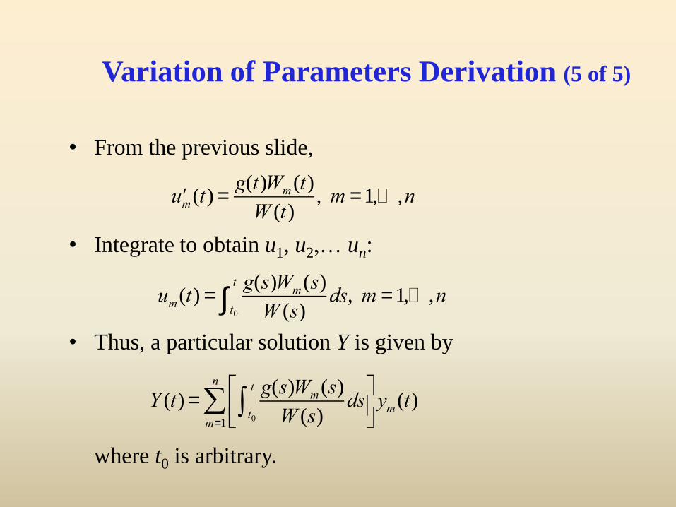
• From the previous slide,

• Integrate to obtain u1, u2,… un:

• Thus, a particular solution Y is given by

where t0 is arbitrary.

¢um(t) =

g(t)Wm(t)

W (t), m = 1,… ,n

um(t) =

g(s)Wm(s)

W (s)ds

t0

t

ò , m = 1,… ,n

Y (t) =g(s)Wm (s)

W (s)ds

t0

t

òé

ëê

ù

ûú ym (t)

m=1

n

å

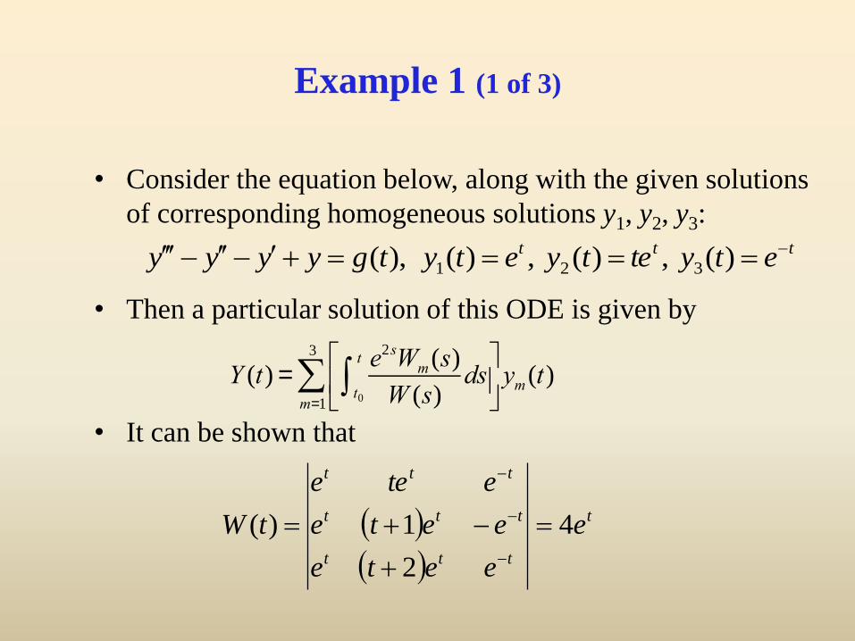
Example 1 (1 of 3)

• Consider the equation below, along with the given solutions

of corresponding homogeneous solutions y1, y2, y3:

• Then a particular solution of this ODE is given by

• It can be shown that

ttt etytetyetytgyyyy )(,)(,)(),( 321

Y (t) =e2sWm (s)

W (s)ds

t0

t

òé

ëê

ù

ûú ym (t)

m=1

3

å

t

ttt

ttt

ttt

e

eete

eete

etee

tW 4

2

1)(

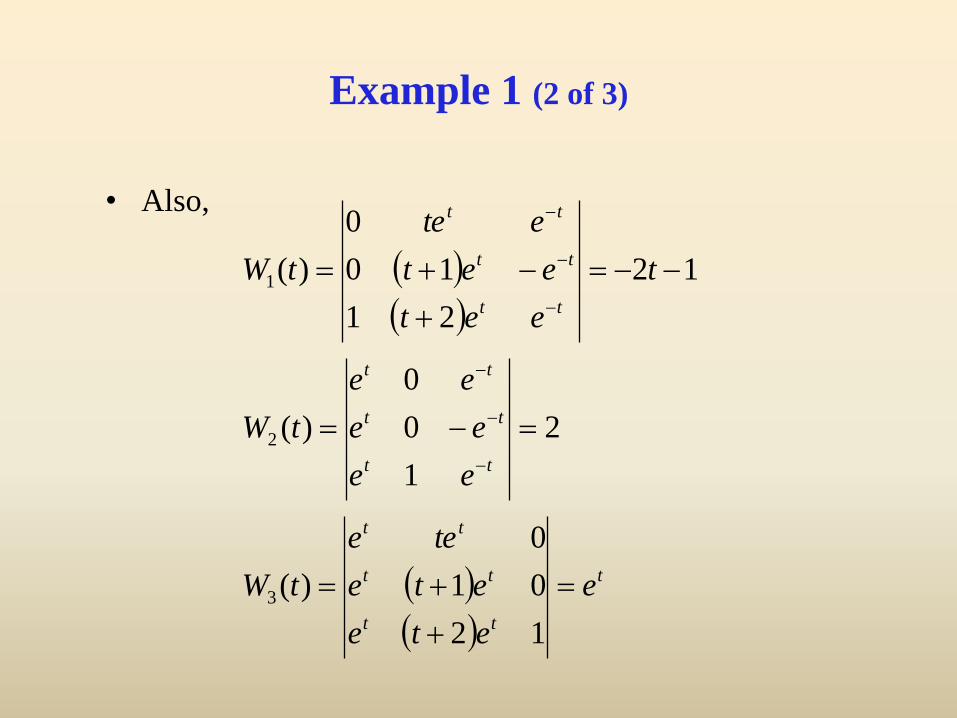
Example 1 (2 of 3)

• Also,

t

tt

tt

tt

tt

tt

tt

tt

tt

tt

e

ete

ete

tee

tW

ee

ee

ee

tW

t

eet

eet

ete

tW

12

01

0

)(

2

1

0

0

)(

12

21

10

0

)(

3

2

1

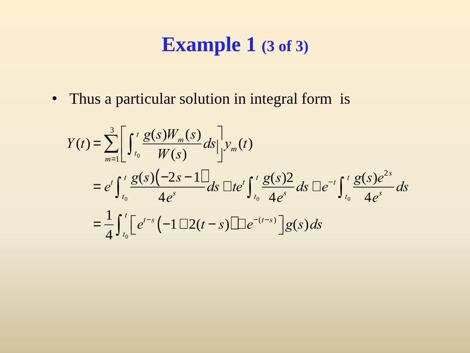
Example 1 (3 of 3)

• Thus a particular solution in integral form is

Y (t) =g(s)Wm (s)

W (s)ds

t0

t

òé

ëê

ù

ûú ym (t)

m=1

3

å

= etg(s) -2s -1( )

4esds

t0

t

ò + tetg(s)2

4esds

t0

t

ò + e-t g(s)e2s

4esds

t0

t

ò

=1

4et-s -1+ 2(t - s)( ) + e-(t-s)éë ùûg(s)ds

t0

t

ò