Boyce/DiPrima 9th ed, Ch 2.8: The Existence and Uniqueness TheoremElementary Differential Equations and Boundary Value Problems, 9th edition, by William E. Boyce and Richard C. DiPrima, ©2009 by John Wiley & Sons, Inc.

The purpose of this section is to prove Theorem 2.4.2, the fundamental existence and uniqueness theorem for first order initial value problems. This theorem states that under certain conditions on f(t, y), the initial value problem

has a unique solution in some interval containing .

First, we note that it is sufficient to consider the problem in which the point is the origin. If some other initial point is given, we can always make a preliminary change of variables, corresponding to a translation of the coordinate axes, that will take the given point into the origin.

00 )(),,(' ytyytfy

0t

),( 00 yt

Theorem 2.8.1

If f and are continuous in a rectangle R: |t| ≤ a, |y| ≤ b, then there is some interval |t| ≤ h ≤ a in which there exists a unique solution of the initial value problem

We will begin the proof by transforming the differential equation into an integral equation. If we suppose that there is a differentiable function that satisfies the initial value problem, then is a continuous function of t only. Hence we can integrate from the initial value t = 0 to an arbitrary value t, obtaining

yf /

0)0(),,(' yytfy

)(ty

)(ty )](,[ ttf

))(,(),(' ttfytfy

)](,[)(0t

dsssft

Proving the Theorem for the Integral Equation

It is more convenient to show that there is a unique solution to the integral equation in a certain interval |t| ≤ h than to show that there is a unique solution to the corresponding differential equation. The integral equation also satisfies the initial condition.

The same conclusion will then hold for the initial value problem

as holds for the integral equation.

abledummy vari a is 0)0()](,[)(0

sdsssftt

0)0(),,(' yytfy

The Method of Successive ApproximationsOne method of showing that the integral equation has a unique solution is known as the method of successive approximations or Picard’s iteration method. We begin by choosing an initial function that in some way approximates the solution. The simplest choice utilizes the initial condition

The next approximation is obtained by substituting for into the right side of the integral equation. Thus

Similarly,

And in general,

)](,[)(0t

dsssft

0)(0 t1 )(0 s

)(s ]0,[)](,[)(

00

01 tt

dssfdsssft

)](,[)(0

12 t

dsssft

)](,[)(0

1

t

nn dsssft

Examining the Sequence

As described on the previous slide, we can generate the sequence with

Each member of the sequence satisfied the initial condition, but in general none satisfies the differential equation. However, if for some n = k, we find , then is a solution of the integral equation and hence of the initial value problem, and the sequence is terminated.

In general, the sequence does not terminate, so we must consider the entire infinite sequence. Then to prove the theorem, we answer four principal questions.

)](,[)(0

1

t

nn dsssft

)](,[)( and0)(0

10

t

nn dsssftt

,...,...,,,}{ 210 nn

)()(1 tt kk )(tk

Four Principal Questions about the Sequence

1. Do all members of the sequence exist, or may the process break down at some stage?

2. Does the sequence converge?

3. What are the properties of the limit function? In particular, does it satisfy the integral equation and hence the corresponding initial value problem?

4. Is this the only solution or may there be others?

To gain insight into how these questions can be answered, we will begin by considering a relatively simple example.

)](,[)(0

1

t

nn dsssft

}{ n

Example 1: An Initial Value Problem (1 of 6)

We will use successive approximations to solve the initial value problem

Note first that the corresponding integral equation becomes

The initial approximation generates the following:

0)0(),1(2' yyty

)](1[2)(0 t

dssst

0)(0 t

6/2/]22(]2/1[2)(

2/]22(]1[2)(

2]01[2)(

642

0 0

53423

0 0

42322

0 0

21

tttdssssdsssst

ttdsssdssst

tdssdsst

t t

t t

t t

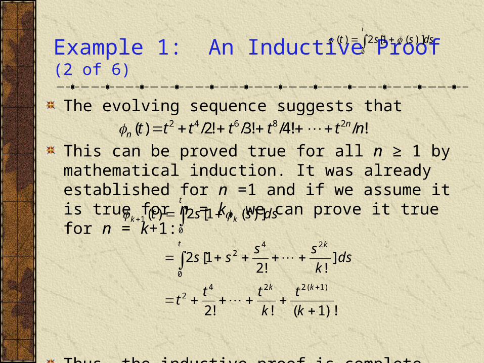
Example 1: An Inductive Proof (2 of 6)

The evolving sequence suggests that

This can be proved true for all n ≥ 1 by mathematical induction. It was already established for n =1 and if we assume it is true for n = k, we can prove it true for n = k+1:

Thus, the inductive proof is complete.

!/!4/!3/!2/)( 28642 ntttttt nn

)](1[2)(0 t

dssst

)!1(!!2

]!!2

1[2

)](1[2)(

)1(2242

0

242

0

1

k

t

k

ttt

dsk

ssss

dssst

kk

t k

t

kk

Example 1: The Limit of the Sequence (3 of 6)

A plot of the first five iterates suggests eventual convergence to a limit function:

Taking the limit as n→∞ and recognizing the Taylor series and the function to which it converges, we have:

2 1 0 1 2t

1

2

3

4

5t

)(1 t

)(2 t)(5 t

!/!4/!3/!2/)( 28642 ntttttt nn

1!!

lim)(lim2

1

2

1

2

t

k

kn

k

k

nn

ne

k

t

k

tt

Example 1: The Solution (4 of 6)

Now that we have an expression for

let us examine for increasing values of k in order to get a sense of the interval of convergence:

The interval of convergence increases as k increases, so the terms of the sequence provide a good approximation to the solution about an interval containing t = 0.

1)(lim2

tn

net

1!!

lim)(lim)(2

1

2

1

2

t

k

kn

k

k

nn

ne

k

t

k

ttt

)()( tt k

3 2 1 1 2 3t

0 .5

1 .0

1 .5

2 .0t

k=1→

←k=10

← k=20

Example 1: The Solution Is Unique (5 of 6)

To deal with the question of uniqueness, suppose that the IVP has two solutions . Both functions must satisfy the integral equation. We will show that their difference is zero:

For the last inequality, we restrict t to 0 ≤ t ≤ A/2, where A is arbitrary, then 2t ≤ A.

)( and )( tt

)](1[2)(0 t

dssst

t

tt

t t

dsssA

dssssdssss

dsssdssstt

0

00

0 0

)()(

)()(2)]()([2

)](1[2)](1[2)()(

Example 1: The Solution Is Unique (6 of 6)

It is now convenient to define a function U such that

Notice that U(0) = 0 and U(t) ≥ 0 for t ≥ 0 and U(t) is differentiable with . This gives:

The only way for the function U(t) to be both greater than and less than zero is for it to be identically zero. A similar argument applies in the case where t ≤ 0. Thus we can conclude that our solution is unique.

t

dssstU0

)()()(

)()()(' tttU

0for 0)(0)(0))((

eby gmultiplyin and 0)()(' -At

ttU tUe'tUe

tAUtU-At-At

t

dsssAtt0

)()()()(

Theorem 2.8.1: The First Step in the Proof

Returning to the general problem, do all members of the sequence exist? In the general case, the continuity of f and its partial with respect to y were assumed only in the rectangle R: |t| ≤ a, |y| ≤ b. Furthermore, the members of the sequence cannot usually be explicitly determined.

A theorem from calculus states that a function continuous in a closed region is bounded there, so there is some positive number M such that |f(t,y) |≤ M for (t, y) in R.

Since , the maximum slope for any function in the sequence is M. The graphs on page 117 of the text indicate how this may impact the interval over which the solution is defined.

Mttft nnn ))(,()(' and 0)0(

t

nn dsssft

yytfy

0

1 )](,[)(

0)0(),,('

Theorem 2.8.1: The Second Step in the Proof

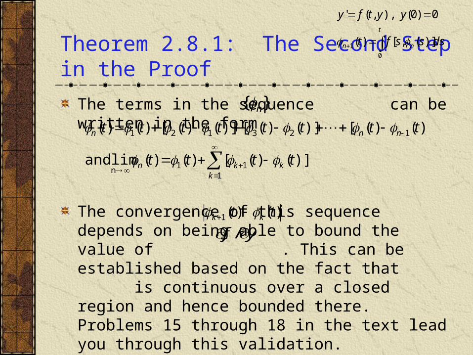
The terms in the sequence can be written in the form

The convergence of this sequence depends on being able to bound the value of . This can be established based on the fact that is continuous over a closed region and hence bounded there. Problems 15 through 18 in the text lead you through this validation.

}{ n

111

n

123121

)]()([)()(lim and

)]()([)]()([)]()([)()(

kkkn

nnn

tttt

tttttttt

)()(1 tt kk

yf /

t

nn dsssft

yytfy

0

1 )](,[)(

0)0(),,('

Theorem 2.8.1: The Third Step in the Proof

There are details in this proof that are beyond the scope of the text. If we assume uniform convergence of our sequence over some interval |t| ≤ h ≤ a and the continuity of f and its first partial derivative with respect to y for |t| ≤ h ≤ a , the following steps can be justified:

t

t

nn

t

nn

t

nn

nn

dsssf

dsssfdsssf

dsssftt

0

00

0

1

)](,[

)](lim,[)](,[lim

)](,[lim)(lim)(

t

nn dsssft

yytfy

0

1 )](,[)(

0)0(),,('

Theorem 2.8.1: The Fourth Step in the Proof

The steps outlined establish the fact that the functionis a solution to the integral equation and hence to the initial value problem. To establish its uniqueness, we would follow the steps outlined in Example 1.

We conjecture that the IVP has two solutions: . Both functions have to satisfy the integral equation and we show that their difference is zero using the inequality:

If the assumptions of this theorem are not satisfied, you cannot be guaranteed a unique solution to the IVP. There may be no solution or there may be more than one solution.

)(t

)( and )( tt

t

dsssAtt0

)()()()(

t

dsssfty

yytfy

0

)](,[)(

0)0(),,('