BOUNDED-RATIONAL BEHAVIOR BY NEURAL NETWORKS … · 2001-08-17 · BOUNDED-RATIONAL BEHAVIOR BY...

BOUNDED-RATIONAL BEHAVIOR BY NEURAL NETWORKS IN NORMALFORM GAMES

DANIEL J. ZIZZO AND DANIEL SGROI

Abstract. This paper presents a neural network model developed to simulate the endogenous

emergence of bounded-rational behavior in normal-form games. There exists an algorithm which,

if learnt by a neural network, would enable it to perfectly select Nash equilibria in never before

seen games. However, …nding this algorithm is too complex a task for a biologically plausible

network, and as such it will instead settle for converging to an approximation to Nash in a subset

of games. We employ computer simulations to show that Nash equilibria are found approximately

60% of the times, and to characterize the behavioral heuristics acquired by the bounded-rational

agent. Pure sum of payo¤s dominance, and the best response to this strategy, get closest to

predicting the network’s behavior.

Keywords: rationality, learning, neural networks, normal form games, complexity

JEL Classi…cation Codes: C72, D00, D83

1. Introduction

Consider a naive agent thrown into a world of Nash equilibrium players. For example, he may

be an infant who, …rst, starts playing games with parents and other relatives, and later with a

larger and larger circle of people; he also observes other people playing games. He does not always

face the same game: on the contrary, he either plays or observes other subjects playing a wide

range of games. The outcome of these repeated encounters is all the feedback he gets: there is

no one explicitly teaching him game theory. Will he learn to play Nash strategies right away as

he grows up, when facing games never encountered before? If yes, at what success rate? In this

paper we provide an analytical and simulated neural network model of learning by example: our

Date: 20th March 2001.Various incarnations of this paper have received the comments and the advice of Michael Bacharach, Kalyan Chatter-jee, Vince Crawford, Huw Dixon, Jim Engle-Warnick, Susan Hurley, Gerry Mackie, Meg Meyer, Matthew Mulford,Raimondello Orsini, Andrew Oswald, Michael Rasmussen, Antonio Santamaura and participants in seminars in Ox-ford and Cambridge. D. J. Zizzo is particularly responsible for the conception, simulation and econometric testingof the network; D. Sgroi is particularly responsible for the more analytical elements of the paper. This notwith-standing, the entire paper is fully the result of a concerted e¤ort. D. Sgroi would like to acknowledge funding fromthe ESRC and AEA Technology. Neural network simulations were made using the TLearn software package (seeMacleod, Plunkett, and Rolls (1998)).

1

2 DANIEL J. ZIZZO AND DANIEL SGROI

…ndings suggest that the agent will endogenously learn rules of thumb allowing him to perform in

a satis…cing way when playing new games. The rules of thumb are learnt endogenously insofar

as the agent’s behavior is reinforced according to Nash (he always plays with Nash players). This

is an example of emergent bounded-rational behavior as in Simon (1955) or Simon (1959): rather

than playing the optimal strategy, the agent achieves a satis…cing solution. Moreover, this is a

model of bounded-rational behavior in games in which, di¤erently from other models, for example,

Osborne and Rubinstein (1998), rules of thumb emerge endogenously as a result of the learning

process rather than being exogenously super-imposed on the agent.

The issue of the learnability of Nash equilibria play is also relevant in its own right. Playing

a Nash strategy in a game has long been thought a bare minimum requirement for rational play

in games. The challenge is to provide “a compelling argument for Nash equilibrium” (Mailath

(1998), p. 1351). In the behavioral reinforcement paradigm, what we typically have are agents

capable of reaching Nash equilibrium (or otherwise) in speci…c games, after a feasible long-run

dynamic path as in Roth and Erev (1995). In the evolutionary game theory paradigm, a good deal

of recent work has gone into justifying Nash equilibrium as a stable point in a dynamic learning

or evolutionary process (for example, Young (1993)); yet, by itself it does not provide structural

models of learning as Mailath (1998) is at pains to point out. This has not gone unquestioned.

Furthermore, what much of the work in both of these paradigms has in common is an emphasis on

learning to play a Nash strategy in a particular game. Start with an arbitrary strategy in a game

and determine whether agents converge to playing Nash strategies, and thus a Nash equilibrium,

in the long-run. This paper is very di¤erent, with the emphasis being placed on how reasonable

Nash behavior is in play across a number of games, or throughout a player’s economic life. An

implication of this is that these models typically make no prediction, or predict naive behavior,

when new games are faced.1 Conversely, here the stress will be on the ability of the experienced

agent to play in a non-naive way in games never encountered before, and even belonging to classes

of games never encountered before. The decision algorithm used by the player is formed out of a

series of observed examples, the result being a decision-rule in which the emphasis is on learning

how to play games in general.

If Nash is found to be non-learnable in some important respect, then the focus is bound to shift

to the equally important question of what kind of decision-rule a bounded-rational agent would

tend to learn as an endogenous outcome of the learning process. This paper models economic

situations through normal form games: in relation to this class of games, recent experimental

evidence highlights the importance of two bounded-rational rules, ‘Naive’ and ‘L2’ Costa-Gomes,

1Stahl (1998) provides an exception.

BOUNDED-RATIONAL BEHAVIOR BY NEURAL NETWORKS IN NORMAL FORM GAMES 3

Crawford, and Broseta (2000). A Naive player assumes that the co-player is behaving randomly

and so simply picks up the action corresponding to the highest sum of possible payo¤s: this

corresponds to ‘level 1’ thinking in Stahl and Wilson (1995). A L2 (‘level 2’) player assumes

that the other player follows Naive, and best responds accordingly. We verify how the knowledge

acquired by the bounded-rational agents trained on Nash play is related to Naive, L2 and a set

of other non-Nash algorithms.

In our paper agents are modelled using neural networks. We consider the interaction between

a neural network player and a population of Nash players. We make use of the evolutionary

stability properties of Nash equilibrium to assert the optimality of Nash play by network and

non-network players alike.2 On these grounds, the network is exposed to a series of example

games where the Nash choice is highlighted as the optimal action.3 Then the trained network

faces a new series of games and is left to choose what strategies it sees …t. A neural network could

in theory learn to play games never seen before in a fully rational way, picking Nash equilibria at

the very …rst attempt, having been trained on a set of example games. However, if we use the most

standard learning algorithm used in neural network research, and assert the need for a minimum

amount of biological and cognitive plausibility, we can show that the Nash equilibrium learning

problem is too complex for the neural network. The basic intuition behind this learning algorithm

- backpropagation - is that of psychological reinforcement: the economic decision-maker tries to

learn how to perform better in the task, and the more disappointing the outcome (relative to the

“correct” outcome), the deeper the change in connection weights will be. A neurotransmitter,

dopamine, plays a role in biological neural networks that may be analogous to that of the teacher

providing feedback on the “correct” outcome in the backpropagation algorithm: the activation

level of dopamine neurons might tell the agent how to adapt its behavior to successfully deal

with a task (Zizzo (2001)). This does not mean that backpropagation is a biologically plausible

algorithm; still, it is likely to provide an upper bound to what is biologically plausible in relation to

2Later work might usefully explore the interaction between competing players drawn from a population entirelycharacterized by neural network players, though the optimality of playing Nash strategies in such a population isnot so certain.3More generally, we might interpret rationality as utility maximization rather than the play of a Nash equilibriumstrategy. However, within the speci…c framework of strategic interaction we cannot judge what utility maximizationwill entail without a set of beliefs concerning the opponent’s play. With this in mind, Nash equilibrium constitutesthe most widely accepted form of rational play; furthermore focusing on Nash equilibrium enables us to both addressgeneral questions of rationality and attempt to resolve Mailath’s need for a structural model which justi…es thewidespread use of Nash equilibrium. This does leave the way open to examine simple utility maximisation in anon-strategic framework, and compare results.


networks of any given size (Macleod, Plunkett, and Rolls (1998)).4 More importantly, the usage of

backpropagation is justi…ed by the amount of psychological evidence that has been explained using

models that employ this algorithm, for example in relation to pattern recognition, categorization

and child development (see Zizzo and Sgroi (2000) for some references). Conversely, augmented

learning algorithms, of the kind used by White (1992) to show learnability, have no pretence of

either biological or psychological plausibility (White (1992), p. 161). Hence, the non-learnability

result should be taken seriously: it cannot be easily dismissed as an arti…cial product of too weak

a learning rule.

Computer simulations were made using a network that plays (up to) 3£3 games. We …nd that

the trained network is able to …nd pure Nash equilibria of games never encountered before around

60% of the times, an empirically reasonable success rate as shown in Stahl and Wilson (1994).

This provides some support for Nash equilibrium play: still, it is considerably less than 100%.

The non-learnability result implies that, in practice, a neural network is much more likely to

learn a local error-minimizing algorithm or LMA. This is an interesting result insofar as one

believes that game playing is usually something that is not explicitly taught, but rather implicitly

learnt by repeated encounters with game instances.5 The LMA is an algorithm that, if followed,

minimizes the network’s error in a subset, but only in a subset, of cases. LMAs are interesting

because they correspond to one or more behavioral heuristics that the bounded-rational agent

has endogenously picked up to perform in a satisfacing way on the decision problem (see Sgroi

(2000)).

We characterize the LMA achieved by the trained network in two ways: by simply analyzing

the fraction of choices that are describable by non-Nash algorithms, and by developing simple

econometric techniques based on regression on the network error and on the decisiveness of the

network’s choice. The two kinds of analyses, taken together, give strong support to Naive and L2 as

the non-Nash algorithms getting closest to the LMA that the Nash-trained network has actually

learnt. This is in agreement with Costa-Gomes, Crawford and Broseta’s (2000) experimental

results: this correspondence is the more striking because 3 £ 3 games are not among the games

they use in their experiment. The network displays some strategic awareness, but this is not

4This is not only because of the need for feedback on “correct” outcomes, but also because, as we shall see,backpropagation adjusts individual connection weights using global information on how to best allocate outputerror.5This ‘implicit learning’ assumption is defended in Zizzo (2000a). An implication of this assumption is that Costa-Gomes, Crawford and Broseta’s (2000) result that telling people explicitly how to play games has a signi…cant e¤ecton behavior is not really relevant for this paper: few people in the real world have ever studied game theory, andeven fewer remember what they might have read in a textbook. Neural networks are useful to model implicit, notexplicit learningShanks and St. John (1994).


unbounded. It goes for high payo¤ values. It takes into account potential trembles due to the

temptation of the other player of deviating from Nash. It plays better in higher stakes games,

particularly if there is more con‡ict of interests between itself and the other player. The trained

network’s behavioral heuristics, including its reliance on L2 and Naive, carry over to a relevant

degree when it faces not just new games, but new classes of games, namely games with multiple

and zero pure Nash equilibria. Moreover, networks trained on di¤erent games - all with a unique

pure Nash equilibrium -, are able to coordinate on the same focal solution, when encountering

games with multiple equilibria.

Although neural networks have been used in the past as econometric tools, this is not the spirit

in which they are used in this paper: we conceive of our neural network as a model of decision-

making processes, allowing us to study how a toolkit of bounded-rational knowledge emerges

endogenously, simply as the outcome of the agent learning to cope with too di¢cult a problem.

This improves both our understanding of what a model of bounded rationality should look like,

and of what kind of bounded rationality behavior we should at best expect from human agents,

who are certainly in a less ideal position to learn than the networks in this paper.6

Computer simulations employing neural networks are now a standard way to model categoriza-

tion and learning in computer science, engineering and cognitive psychology. As yet, however,

relatively little has been done within game theory to capitalize on this research. Rubinstein

(1993) uses perceptrons to capture the notion of a limit to forward-looking behavior in monopo-

listic competition; Cho and Sargent (1996) use networks for encoding dynamic strategies. None

of this research uses computer simulations. Conversely, we believe that computer simulations can

be helpful to study what strategies are likely to be encoded in a network as a result of repeated

exposure to examples, rather than what strategies can in principle be encoded. Macy (1996) is

an early example of this, but only in relation to a speci…c game, namely the Prisoner’s Dilemma.

The rest of this paper is organized as follows. Part I of the paper encompasses sections 2

through 4, dealing with mainly theoretical issues. Section 2 presents the game to be played,

section 3 formally presents the neural network player, and section 4 examines the learnability of

the Nash solution by the neural network. Part II of the paper, incorporating sections 5 through 8,

addresses what the network actually learns, using computer simulations and simple econometric

techniques. Section 5 introduces the simulated neural network, and details several alternatives to

the Nash solution concept as possible alternative candidates for the neural network’s behavior.

Computer simulations, and an econometric analysis of the results, are described in section 6 for

6This is because human agents may not be facing a population of Nash players.


games with unique equilibria, section 7 for games with multiple equilibria, and section 8 for games

with no equilibria. Section 9 concludes.

Part I: The Theory of Neural Network Learning in Games

Neural networks can be loosely de…ned as arti…cial intelligence models inspired by analogy with

the brain and realizable in computer programs. They typically learn by exposure to a series of

examples (a training set), and adjustment of the strengths of the connections between its nodes.

They are then able to do well not only on the original training set, but also when facing problems

never encountered before.

2. The Model

This section is devoted to a sequence of de…nitions, and a thorough explanation of the neural

network model. The notion of random games will also be introduced, the key feature of which is

that each game in a sequence will not have been played before by any player. This captures the

notion of play in a new and changing environment: it rules out standard theories of evolutionary

learning in which the game to be repeatedly played is essentially unchanging.

2.1. Basic De…nitions. For the purposes of this paper, a random game, G, is de…ned as a 3£ 3normal form game of full information with a unique pure strategy Nash equilibrium and randomly

determined payo¤s taken from a uniform distribution with support [0; 1]. More formally we can

de…ne the simple game by a list G =N; fAi; uigi2N

®. We will restrict the number of players,

indexed by i, to N = 2. Ai describes player actions available to a player in role i, with realized

actions given by ai 2 Ai. In each game we consider the set of feasible actions available to each

player to be of size 3. Feasible action combinations are given by A = A1 £ A2. Payo¤s for both

players are given by ui : Ai 7! R which is a standard von Neumann-Morgenstern utility function.

Payo¤s are bounded, so 9Q ¸ 0 such that j ui (a) j· Q for all a. More speci…cally we consider

the payo¤s to be randomly drawn from a uniform (0; 1) and then revealed to the players before

they select an action, so 8i;a, supui (ai) = 1. We will place one further restriction on the game,

by requiring the existence of a single unique pure strategy Nash equilibrium. To summarize:

De…nition 1. A random game is a list G =N; fAi; uigi2N

®, such that N = 2 players meet to

play a game playing realized action ai 2 Ai, where three action choices are allowed. The values of

the payo¤s, ui : Ai 7! R are randomly drawn from a uniform (0; 1), made known to the players

before the game starts, and form a standard von Neumann-Morgenstern bounded utility function.


Now consider a population of Q players playing a series of random games, indexed by t 2 N++.

We consider a pair to be drawn from our population and then forced to play a given random game.

De…ne the unique pure strategy Nash strategy to be ®i 2 Ai where a Nash strategy is de…ned as

the unique choice of pure strategy by player i which, when taken in combination with the Nash

strategy chosen by the other member of the drawn pair, form the unique Nash equilibrium in the

random game. So de…ning the speci…c Nash strategy for player i in a given random game to be

®i, and indexing the second player by j we have:

ui (ai = ®i j aj = ®j) > ui (ai 6= ® j aj = ®j)(1)

We can say immediately that:

Proposition 1. Player i, taken from the population of size Q, wishing to maximize ui, must play

the unique Nash strategy when drawn to play in G, and therefore the outcome will be the unique

Nash equilibrium in G.

This is trivial given the de…nition of a Nash equilibrium. To say more we must …rst de…ne an

evolutionary stable strategy:

De…nition 2. Let x and y be two mixed strategies from the set of mixed strategies in G. Now let

u (x; y) de…ne the utility associated with the play of strategy x given the play of strategy y by the

other player. The strategy x is said to be an evolutionary stable strategy (ESS) if 8y 9"y > 0 s.t.

when 0 < " < "y:

u (x; (1¡ ")x+ "y) > u (y; (1¡ ")x+ "y)(2)

Now we can show that:

Proposition 2. The unique Nash strategy of G is an evolutionary stable strategy (ESS).

Proof. This proof is simply a restatement of the well-known result that local superiority implies

evolutionary stability. Firstly, G has a unique Nash strategy by de…nition. Call this strategy ®i

for player i. Now we know that u (®i j aj = ®j) > u (ai j ai 6= ®i; aj = ®j) so by the uniqueness

of ®i we know that any mix of ®i with ai 6= ®i will reduce u (®i; aj) where u (ai; aj) is the payo¤

to player i from action ai 2 A given player j plays aj 2 A. Therefore the Nash equilibrium of

G must be strict. By strictness we know that u (®i; aj) > u (¯i; aj) where ¯i 6= ®i. This in turn

implies local superiority, so:

lim"!0

©(1¡ ")u (®i; ®j) + "u

¡®i; ¯j

¢ª> lim

"!0

©(1¡ ")u (¯i; ®i) + "u

¡®i; ¯j

¢ª


By linearity of expected utility in probabilities this implies:

u¡®i; (1¡ ")®j + "¯j

¢> u

¡¯i; (1¡ ")®j + "¯j

¢for " ! 0

Which is simply a restatement of the de…nition of an ESS given in de…nition 2.

We have a simple notion of a population of players playing Nash against each other and per-

forming well in terms of their payo¤s. We now consider the mutation of a proportion ° of the

population into neural network players. By proposition 2 we know the remaining population will

continue to play Nash strategies, if we let ° ! 0. We can retain this property by letting Q ! 1and setting ° to be …xed at a number strictly above zero, but …nite. In particular, we can con-

sider a single member of the population to be a neural network player, but let Q ! 1 to bring

° arbitrarily close to zero. We can now examine the actions of this single neural network player

content in the knowledge that all other players will continue to play Nash strategies. Therefore,

we can be assured that the neural network’s best reply to the population will be to play a Nash

strategy.

3. The Neural Network Player

Let us start with an intuitive account of the single neural network player in G. Consider a

young economic agent with no prior experience of play in any game. This agent will, however,

have a base of experience derived from a prior period spent learning “how to play”. We might

imagine a student’s time at school or observation of how older members of the population play

certain games. This agent has a store of observed example games, none of which will necessarily

…t exactly with any game he will face in the future, but which might share certain similarities.

We capture this notion of learning by example prior to entry into the economy, or marketplace

of games, through the use of a neural network. We …rst “train” the agent by subjecting him to a

series of example games with given actions and payo¤s, we require him to be a utility maximizer,

and then use a form of backpropagation to allow him to develop a form of pattern recognition

which will enable him to “learn by example”, and attempt to learn to play the Nash strategy

in order to maximize his payo¤. The question we ask is: can we introduce the network to a

marketplace modelled by a sequence of random games …lled with Nash players and expect the

network to learn to play Nash? The key point is that he will be most unlikely to ever play the

same game twice and will be most unlikely ever to have seen the identical game in his training

period, so will his pattern recognition abilities be su¢cient for him to intuitively recognize the

Nash strategy in an entirely new game and play it? We are now switching out of the evolutionary


framework and focusing on the play of a single player rather than the behavior of the population

in general. We …rst need to add some formal de…nitions.

3.1. De…ning the Network. Consider a neural network, or more simply C to be a machine

capable of taking on a number of states, each representing some computable functions mapping

from input space to output space, with two hidden layers of further computation between input

and output.7 The following de…nition formalizes this.

De…nition 3. De…ne the neural network as C = h; X; Y; F i where is a set of states, X µ Rn

is a set of inputs, Y is a set of outputs and F : £ X 7! Y is a parameterized function. For

any ! the function represented by state ! is h! : X 7! Y given by h! (x) = F (!; x) for an input

x 2 X. The set of functions computable by C is fh! : ! 2 g, and this is denoted by HC .

Put simply, when the network, C, is in state ! it computes the function h! providing it is

computable. In order to reasonably produce answers which correspond to a notion of correctness

(in this case the unique Nash strategy in a 3£ 3 game), we need to train the network. First we

will consider the form of the network in practice, and start by de…ning an activation function.

De…nition 4. An activation function for node i of layer k in the neural network C is of the

logistic form

aki =

1

1¡ exp³

¡Pj wkiju

k¡1ij

´(3)

where ukij is the output of node j in layer k ¡ 1 sent to node j in layer k, and wij is the weight

attached to this by node i in layer k. The total activation ‡owing into node i,P

j wkijuk¡1

ij , can

be simply de…ned as ti.

Consider a set of 18 input nodes each recording and producing as output a di¤erent value

from the vector xk =¡x1

k; :::; x18k

¢. This neatly corresponds to the payo¤s of a 3£ 3 game. Now

consider a second set of 36 nodes (the …rst hidden layer). Each node in this second layer receives

as an input the sum of the output of all 18 input nodes transformed by the activation function

of node i in layer 2. All of the nodes in the second layer send this output a2i to all nodes in the

second hidden layer, which weights the inputs from all i of the …rst hidden layer, by the activation

function to produce a3i . These numbers are sent to the …nal layer of two nodes to produce an

output y which forms a 2-dimensional vector which represents the choice of strategy in a 3 £ 3

7Hidden layers can be thought of as intermediate layers of computation between input and output. Since we seethe input go in, and the output come out, but do not directly see the activity of intermediate layers, they are insome sense hidden.


game. To explain this representation of a strategy in a 3£ 3 game for the row player, the vector

(1; 0) would imply the pure Nash strategy is the top row, (0; 1) would imply the middle row, and

(0; 0) the bottom row.

3.2. Training the Network. Training essentially revolves around …nding the set of weights that

is most likely to produce the desired output. During training C receives a sequence of random

games until some stopping rule determines the end of the training at some round T (discussed

below). The training sample consists of M random games. If T > M , then (some or all of) the

random games in M will be presented more than once.

Let us formally de…ne the training sample. The vector xk =¡x1

k; :::; x18k

¢consists of 18 real-

valued numbers drawn from a uniform (0; 1) representing the payo¤s of a 3 £ 3 game. It is

recorded in the …rst set of input nodes, and then sent and transformed by the two hidden nodes

before an output y, a two-dimensional vector, is produced and represented in the …nal layer.

This is repeated M times with a new set of inputs xk and outputs yk. Assume that each vector

xk is chosen independently according to a …xed probability distribution PT on the set X. The

probability distribution is …xed for a given learning problem, but it is unknown to C, and for our

purposes will be taken to be a uniform (0; 1). The information presented to C during training

therefore consists only of several sequences of numbers.

De…nition 5. For some positive integer m, the network is given a training sample:

xM =¡¡

x11; :::; x18

1

¢;¡x1

2; :::; x182

¢; :::;

¡x1

M ; :::; x18M

¢¢= (x1; x2; :::; xM) 2 XM

The labelled examples xi are drawn independently according to the probability distribution PT . A

random training sample of length M is an element of XM distributed according to the product

probability distribution P M .

Assume that T > M . In this case, training might be sequential : after q £ M rounds (for any

positive integer q s.t. q £ M < T ), M is presented again, exactly in the same order of games.

If training is random without replacement, it is less restricted to the extent that the order in

which the random games are presented each time is itself random. If training is random with

replacement, in each round the network is assigned randomly one of the random games in M ,

until round T .

Having selected a sample sequence of inputs, x, and determined the unique Nash strategy

associated with each, ®, we need to consider how C learns the relationship between the two, to

ensure that its output y will approach the Nash strategy. The method used is backpropagation.

First let us de…ne the error function.


De…nition 6. De…ne the network’s root mean square error " as the root mean square di¤erence

between the output y and the correct answer ® over the full set of q £ M games where individual

games are indexed by i, so our error function is:

" ´Ã

q£MXi=1

(yi ¡ ®i)2

!12

The aim is to minimize the error function by altering the set of weights wij of the connections

between a typical node j (the sender) and node i (the receiver) in di¤erent layers. These weights

can be adjusted to raise or lower the importance attached to certain inputs in the activation

function of a particular node. Backpropagation is a form of numerical analysis akin to gradient

descent search in the space of possible weights. Following Rumelhart, Hinton, and Williams (1986)

we use a function of the form:

4wij = ¡´@"

@wij= ´kipoj(4)

where wij is simply the weight of the connection between the sending node j and receiving node

i. As " is the neural network’s error, @"=@wij measures the sensitivity of the neural network’s

error to the changes in the weight between i and j. There is also a learning rate given by

´ 2 (0; 1]: this is a parameter of the learning algorithm and must not be chosen to be too small

or learning will be particularly vulnerable to local error minima. Too high a value of ´ may also

be problematic as the network may not be able to settle on any stable con…guration of weights.

De…ne @"=@wij = ¡kipojp where ojp is the degree of activation of the sender node ojp. The higher

ojp is, the more the sending node is at fault for the erroneous output, so it is this node we wish

to correct more. kip is the error on unit i for a given input pattern p, multiplied by the derivative

of the output node’s activation function given its input. Calling gip the goal activation level of

node i for a given input pattern p, in the case of the output nodes kip can be computed as:

kip = (gip ¡ oip)f0(tip) = (gip ¡ oip)oip(1¡ oip)(5)

since the …rst derivative f 0(tip) of the receiving node i in response to the input pattern p is equal

to oip(1 ¡ oip) for a logistic activation function. Now assume that a network has N layers, for

N ¸ 2. As above, we call layer 1 the input layer, 2 the layer which layer 1 activates (the …rst

hidden layer), and so on, until layer N the output layer which layer N ¡ 1 activates.

We can now de…ne the backpropagation learning process.


De…nition 7. Using backpropagation, we …rst compute the error of the output layer (layer N)

using equation 5, and update the weights of the connections between layer N and N ¡ 1, using

equation 4. We then compute the error to be assigned to each node of layer N ¡ 1 as a function

of the sum of the errors of the nodes of layer N that it activates. Calling i the hidden node, p the

current pattern and ¯ an index for each node of layer N (activated by i), we can use:

kip = f 0(tip)X

¯

k¯pw¯i(6)

to update the weights between layer N ¡ 1 and N ¡ 2, together with equation 4. We follow this

procedure backwards iteratively, one layer at a time, until we get to layer 1, the input layer.

A variation on standard backpropagation would involve replacing equation 4 with a momentum

function of the form:

4wtij = ¡´

@"t

@wtij

+ ¹ 4 wt¡1ij(7)

where ¹ 2 [0; 1) and t 2 N++ denotes the time index (an example game, vector x, is presented in

each t during training).

Momentum makes connection changes smoother by introducing positive autocorrelation in the

adjustment of connection weights in consecutive periods. The connection weights of the network

are updated using backpropagation until round T . T itself can be determined exogenously by the

researcher, or it can be determined endogenously by the training process, i.e. training may stop

when the network returns the correct output with " lower than a given target value.

4. Inadequate Learning

We have now a clear idea of what the neural network is and the game that the neural network

will face. The training set is simply a sequence of vector pairs (x; y) where the inputs x 2 X

correspond to the set of actions Ai for N players in M random games, and the outputs to the

payo¤s ui : A 7! R for N players for each of the actions. We set M = 2000; N = 2 and restrict

the action set by assuming a 3 £ 3 normal form game. This restriction is done without loss of

generality: potentially any …nite normal form could be modelled in a similar way, while 2 £ 2,

2 £ 3 and 3 £ 2 games count as a subclass of 3 £ 3:8 We then allow the network to play 2000

8While the neural network model was designed with 3 £ 3 games in mind, since all payo¤ values are drawn from auniform [0; 1], it is straightforward to train the current network on 2 £ 2 games, by putting zeros on all the valuesin the third row and third column of each game. Similarly we could construct 2 £ 3 and 3 £ 2 games by placingzeros in the appropriate row or column. The choice of a 3 £ 3 is therefore much more general than the choice of2 £ 2, and can include several interesting and well-known 2 £ 2 games.


further random games never encountered before, selecting a single input and recording a single

output. Since we force each game to contain a unique Nash equilibrium in pure strategies and we

restrict the network’s choice to be in pure strategies, we can then check the network’s success rate

as de…ned by the proportion of times the network selected the Nash strategy to within a given

threshold of mean squared error (as de…ned in de…nition 6). For example if the correct output is

(1; 0) and the neural network returns (0:99; 0) it easily meets an " = 0:05 threshold).

4.1. Incomplete Neural Network Learning. We now need to examine how well a neural

network can do in theory, and fortunately various results exist in the literature to which we

can refer. One of the most well-known results comes from Hornik, Stinchombe, and White (1989)

reprinted in White (1992). Hornik, Stinchombe, and White (1989) show that standard feedforward

networks with only a single hidden layer can approximate any continuous function uniformly on

any compact set and any measurable function arbitrarily well in the p¹ metric, which they de…ne

as follows (in slightly amended form):

De…nition 8. (Hornik, Stinchombe, and White (1989)). Let R be the set of real numbers, and

Br the Borel ¾-…eld of Rr. Let Kr be the set of all Borel measurable functions from Rr to R.

Given a probability measure ¹ on (Rr; Br) de…ne the metric p¹ from Kr £ Kr to R+ by p¹ (f; g)

= inf f" > 0 : ¹ fx :j f (x)¡ g (x) j> "g < "g.

The main result, summarized in theorem 2.4 in Hornik, Stinchombe, and White (1989), e¤ec-

tively concerns the existence of a set of weights which allow the perfect emulation of the algorithm

that the neural network is attempting to learn. There are three potential areas for failure:

1. Inadequate learning, or a failure of the learning dynamic to reach the global error-minimizing

algorithm.

2. Inadequate network size, or insu¢cient hidden units.

3. The presence of a stochastic rather than a deterministic relation between input and target.

Problem 3 can be extended to include poly-random functions (which cannot be distinguished

from random functions by any polynomial approximation) but is still not a problem for the class

of normal form games G. Problem 2 introduces a parallel mechanism for examining bounded-

rational behavior. Along similar lines to the automata literature, we might restrict the number of

hidden units in order to force bounded-rational behavior upon our player. However, regardless of

any attempts to raise the network size to cover for any potential problems, we cannot reasonably

deal with problem 1: it is the problem of inadequate learning and the nature of the learning

algorithm which is the focus of the rest of this section.


4.2. Learning and Learnability. A learning algorithm takes random training samples and

acts on these to produce a hypothesis h 2 H that, provided the sample is large enough is with

probability at least 1¡ ±, "-good (with " de…ned as above) for PT . It can do this for each choice

of "; ± and PT . To de…ne this more formally:

De…nition 9. Suppose that H is a class of functions that map X 7! Y . A learning algorithm

L for H is a function L : [1M=1ZM 7! H from the set of all training samples to H, with the

following property: for any 8p2(0;1);±2(0;1)9 an integer M0 ("; ±) s.t. if M ¸ M0 ("; ±) then, for any

probability distribution PT on Z = X £ Y , if z is a training sample of length M drawn randomly

according to the product distribution P M , then, with probability at least 1 ¡ ±, the hypothesis

L (z) output by L is such that erp (L (z)) < optp (H) + ". More compactly, for M ¸ M0 ("; ±),

P M ferp (L (z)) < optp (H) + "g ¸ 1¡ ±.

To restate in slightly di¤erent terms we can de…ne a function L as a learning algorithm, if 9a

function "0 (M; ±) s:t: 8M;±;PT, with probability at least 1 ¡ ± over z 2 ZM chosen according to

P M , erp (L (z)) < optp (H) + "0 (M; ±), and 8±2(0;1); "0 (M; ±) ! 0 as M ! 1. This de…nition

stresses the role of "0 (M; ±) which we can usefully think of as an estimation error bound for the

algorithm L. A closely related de…nition is:

De…nition 10. We say that H is learnable if 9 a learning algorithm for H.

The function hw can be thought of as representing the entire processing of the neural network’s

multiple layers, taking an input vector x and producing a vector representation of a choice of

strategy. Over a long enough time period we would hope that C will return a set of optimal

weights which will in turn produce the algorithm hw which will select the Nash strategy if 9a learning algorithm for selecting Nash equilibria (H in this case). Or alternatively if we wish

to attain some below perfect success rate, we can do so using a …nite training sample, and the

success rate will grow as the number of examples increases. This all crucially rests on the ability of

backpropagation to pick out the globally error-minimizing algorithm for …nding Nash equilibria.

This now allows us to tightly de…ne the learning problem faced by C.

De…nition 11. C, using the learning algorithm given by de…nition 7 faces a training sample

of size M £ q. The Nash problem is to …nd an algorithm as de…ned in de…nition 9 for which

"0 (M; ±) ! 0 as M ! 1 where the error function " is as de…ned in de…nition 6.

4.3. Finding the Global Minimum. Having established the problem we now need to ver-

ify that the algorithm which successfully collapses "0 (M; ±) to zero is indeed learnable. While

backpropagation is undoubtedly one of the most popular search algorithms currently used to


train feedforward neural networks, it is a gradient descent algorithm and therefore this approach

leads only to a local minimum of the error function (see for example, Sontag and Sussmann

(1989). White (1992), p. 160, makes the point: “...Hoornik et al (1989) have demonstrated that

su¢ciently complex multilayer feedforward networks are capable of arbitrarily accurate approx-

imations to arbitrary mappings... An unresolved issue is that of “learnability”, that is whether

there exist methods allowing the network weights corresponding to these approximations to be

learned from empirical observation of such mappings.” White (1992), chapter 9, theorem 3.1,

provides a theorem which summarizes the di¢culties inherent in backpropagation: he proves that

backpropagation can get stuck at local minima or saddle points, can diverge, and cannot even be

guaranteed to get close to a global minimum. This is not surprising: backpropagation is after all

a gradient descent algorithm.

The problem is exacerbated in the case of our neural network C as the space of possible weights

is so large. Auer, Herbster, and Warmuth (1996) have shown that the number of local minima

for this class of networks can be exponentially large in the number of network parameters. Son-

tag (1995) gives upper bounds for the number of such local minima, but the upper bound is

unfortunately not tight enough to lessen the problem. In fact as the probability of …nding the

absolute minimizing algorithm (the Nash algorithm) is likely to be exponentially small, the learn-

ing problem faced by C falls into a class of problems known in algorithm complexity theory as

NP -hard.9 There exists a literature on the complexity of computing an automaton to play best

response strategies in repeated games (see Gilboa (1988) and Ben-Porath (1990)), but in all cases

the problem examined is one of computing best response algorithms in a repeated game context,

not when facing never before played one-shot games. Nevertheless the literature establishes the

precedent of using algorithm complexity to help determine the reasonableness of certain strategies

(automata) employed by bounded players, and in many cases establishes the hardness of com-

puting Nash strategies. Within the computer science literature there do exist results which are

directly applicable to the problem we examine. Theorem 25.5 from Anthony and Bartlett (1999)

succinctly states the following (in a slightly amended form):

Theorem 1. Problems of the type given in de…nition 11 faced by the class of networks encom-

passing C are NP -hard.

Anthony and Bartlett (1999) chapters 23 to 25, provides various forms of this theorem for

di¤erent types of network including the feedforward class of which C is a member. The following

9For more on the the theory of algorithm complexity and its relationship to neural networks and games, see Sgroi(2000) and Zizzo and Sgroi (2000).


proposition is simply a restatement of theorem 1 with reference to the particular problem faced

by C.

Proposition 3. C supplemented by the backpropagation learning dynamic will not be able to learn

the Nash algorithm in polynomial time.

Gradient descent algorithms attempt to search for the minimum of an error function, and

backpropagation is no exception. However, given the prevalence of local minima, they cannot

consistently solve the problem in de…nition 9 and …nd an absolute minimum. The basins of

attraction surrounding a local minimum are simply too strong for a simple gradient descent algo-

rithm to escape, so looking back to de…nition 9 we cannot expect "0 (M; ±) ! 0 as M ! 1, and

in turn we cannot consider the task facing the network to be learnable in the sense of de…nition

10.10 However, if we were to supplement the algorithm with a guessing stage, i.e. add something

akin to grid search or one of several theorized additions or alternatives to backpropagation, then

we might expect to …nd the absolute minimum in polynomial time.11 To restate this in terms of

the search for an algorithm capable of providing Nash equilibria in never before seen games, back-

propagation cannot do this perfectly, while other far less biologically plausible methods involving

processor hungry guess and verify techniques, can produce consistent results.

So our player will …nd a decision-making algorithm that will retain some error even at the limit,

or to put this an alternative way, we may have to be content with an algorithm which is e¤ective

in only a subclass of games, so it optimizes network parameters only in a small subspace of the

total space of parameters. In the case of normal form games we can summarize this section as:

our player will almost surely not learn the globally error-minimizing algorithm for selecting Nash

equilibria in normal form games. However, we can reasonably assume that some method will be

learned, and this should at least minimize error in some subset of games corresponding to the

domain of some local error-minimizing algorithm.

4.4. Local Error-Minimizing Algorithms. Given that backpropagation will …nd a local min-

imum, but will not readily …nd an absolute minimizing algorithm in polynomial time, we are left

10This is intuitively seen to be reasonable with reference to two results. Fukumizu and Amari (2000) shows thatlocal minima will always exist in problems of this type, and Auer, Herbster, and Warmuth (1996) show that thenumber of local minima for this class of networks is exponentially large in the number of network parameters. Interms of the theory of NP -completeness, we might say the solution could be found in exponential time, but notin polynomial time. For any network with a non-trivial number of parameters, such as C, the di¤erence is greatenough for the term intractable to be applied to such problems.11White (1992), chapter 10, discusses a possible method which can provide learnability, using an application ofthe theory of sieves. However, White (1992), p. 161, stresses: “The learning methods treated here are extremelycomputationally demanding. Thus, they lay no claim to biological or cognitive plausibility.” The method is thereforeuseful for computing environments and practical applications, rather than the modelling of decision-making.


with the question, what is the best our neural network player can hope to achieve? If we believe

the neural network with a large, but …nite training set nicely models bounded-rational economic

agents, but cannot ‡awlessly select Nash strategies with no prior experience of the exact game

to be considered, this question becomes: what is the best a bounded-rational agent can hope to

achieve when faced with a population of fully rational agents?

In terms of players in a game, we have what looks like bounded-rational learning or satis…cing

behavior: the player will learn until satis…ed that he will choose a Nash equilibrium strategy

su¢ciently many times to ensure a high payo¤. We label the outcome of this bounded-rational

learning as a local error-minimizing algorithm (LMA).12

More formally, consider the learning algorithm L, and the ‘gap’ between perfect and actual

learning, "0 (M; ±). Recall that ZM de…nes the space of possible games as perceived by the neural

network.

De…nition 12. If 9 a function "0 (M; ±) s:t: 8M;±;PT, with probability at least 1 ¡ ± over all

z 2 ZM chosen according to P M , erp (L (z)) < optp (H) + "0 (M; ±), and 8±2(0;1); "0 (M; ±) ! 0

as M ! 1 then this function is de…ned the global error-minimizing algorithm (GMA).

This simply states that for all possible games faced by the network, after su¢cient training,

the function will get arbitrarily close to the Nash algorithm,13 collapsing the di¤erence to zero.

This clearly requires an algorithm su¢ciently close to Nash to pick a Nash equilibrium strategy

in almost all games.

De…nition 13. A local error-minimizing algorithm (LMA) will select the same outcome as a

global error-minimizing algorithm for some z 2 ZM , but will fail to do so for all z 2 ZM :

LMAs can be interpreted as examples of rules of thumb that a bounded-rational agent is likely

to employ (for example, Simon (1955) and Simon (1959)). They di¤er from traditionally conceived

rules of thumb in two ways. First, they do select the best choice in some subset of games likely to

be faced by the learner. Second, they are learned endogenously by the learner in an attempt to

maximize the probability of selecting the best outcome. The ‘best’ outcome can be determined

in terms of utility maximization or a reference point, such as the Nash equilibrium.

Part II: Analysis of Neural Network Learning

12For more on this see Sgroi (2000).13The algorithm to …nd pure Nash equilibria in 3 £ 3 games is trivial and not reproduced here. It can be found inZizzo and Sgroi (2000).


The network is unlikely to learn to play Nash at 100% success rate facing new games: it is

facing too complex a problem for it to be able to do so using backpropagation. What is then the

trained network actually learning to do? This is not a question that can be addressed analyti-

cally: however, computer simulations may help, together with simple statistical and econometric

techniques to analyze the results of the simulations.

We …rst focus on the performance of the Nash algorithm and the robustness of the results

to di¤erent parameter combinations: the results validate the unlearnability result in Part 1, but

they also show that the trained network has learnt something. In the following section we deepen

the analysis by analyzing the performance of di¤erent decision algorithms. We then develop an

econometric technique based on a regression analysis on the network error " to investigate what

game features characterize the LMA adopted by the network. Later we modify this econometric

technique to see how the trained network fares on games with zero and multiple pure Nash

equilibria (PNE).

The training set consisted of M = 2000 games with unique PNE. Training was random with

replacement, and continued until the error " converged below 0.1, 0.05 and 0.02, i.e. three conver-

gence levels ° were used: more than one convergence level was used for the sake of performance

comparison. Convergence was checked every 100 games, a number large enough to minimize the

chance of a too early end of the training: clearly, even an untrained or poorly trained network

will get an occasional game right, purely by chance. The computer determined initial connection

weights and order of presentation of the games according to some ‘random seed’ given at the start

of the training. To check the robustness of the analysis, C was trained 360 times, that is once for

every combination of 3 learning rates ´ (0.1, 0.3, 0.5), 4 momentum rates ¹ (0, 0.3, 0.6 and 0.9)

and 30 (randomly generated) random seeds. Convergence was always obtained, at least at the 0.1

level, except for a very high momentum rate.14 We will henceforth call the simulated network C¤

once trained to a given convergence level.

C¤ was tested on a set of 2000 games with unique Nash equilibria never encountered before.15

We considered an output value to be correct when it is within some range from the exact correct

value. If both outputs are within the admissible range, then the answer can be considered correct

(Reilly (1995)). The ranges considered were 0.05, 0.25 and 0.5, in decreasing order of precision.

[insert table 1 here]

14Details on convergence can be found in Zizzo (2000b).15We restricted ourselves to training with games with unique PNE because of the technical need for backpropagationto be able to work with a unique solution. This appeared a lesser evil relative to having to postulate re…nementsto Nash in order to discriminate among multiple equilibria, and hence make the analysis dependent on thesere…nements. Still, the latter might be an interesting avenue to pursue in future research.


Table 1 displays the average performance of C¤ classi…ed by °, ´ and ¹. It shows that C¤

trained until ° = 0:1 played exactly (i.e., within the 0.05 range) the Nash equilibria of 60.03%

of the testing set games, e.g. of 2000 3£ 3 games never encountered before. This …ts well with

the 59.6% average success rate of human subjects newly facing 3£3 games in Stahl and Wilson’s

(1994) experiment, although one has to acknowledge that the sample of games they used was far

from random. With an error tolerance of 0.25 and 0.5, the correct answers increased to 73.47 and

80%, respectively.

Further training improves its performance on exactness - the 0.02-converged C¤ plays exactly

the Nash equilibria of a mean 66.66% of the games - but not on “rough correctness” (the 20%

result appears robust). This suggests (and indeed further training of the network con…rms) that

there is an upper bound on the performance of the network.

Table 1 also shows that, once C converges, the degree it makes optimal choices is not a¤ected

by the combination of parameters used: the average variability in performance across di¤erent

learning rates is always less than 1%, and less than 2% across di¤erent momentum rates. This is

an important sign of robustness of the analysis.

We compared C¤’s performance with three null hypotheses of zero rationality. Null1 is the

performance of the entirely untrained C: it checks whether any substantial bias towards …nding

the right solution was hardwired in the network. Null2 alternates among the three pure strategies:

if C¤’s performance is comparable to Null2, it means all it has learnt is to be decisive on its choice

among the three. Null3 entails a uniformly distributed random choice between 0 and 1 for each

output: as such, it is a proxy for zero rationality. Table 2 compares the average performance of

C¤ with that of the three nulls. Formal t tests for the equality of means between the values of C¤

and of each of the nulls (including Null2) are always signi…cant (P<0.0005). C¤’s partial learning

success is underscored by the fact, apparent from Tables 1 and 2, that when C¤ correctly activates

an output node it is very likely to categorize the other one correctly, while this is not the case for

the nulls.


So it appears that C¤ has learnt to generalize from the examples and to play Nash strategies

at a success rate that is signi…cantly above chance. Since it is also signi…cantly below 100%, the

next question we must address is how to characterize the LMA achieved by the trained network.


5. Alternatives to Nash

Our …rst strategy in trying to characterize the LMA employed by the trained network is to ask

ourselves whether there are simple alternatives to Nash capable of describing what the network

does better than Nash, on the games over which they are uniquely de…ned. Given the robustness

of our analysis in the previous section to di¤erent combinations of ´ and ¹, in this and the next

sections we just focus on the case with ´ = 0:5 and ¹ = 0:16 Hence, for testing we used the

30 networks trained with the 30 di¤erent random seeds but with the same learning (0.5) and

momentum (0) rates. Using these 30 networks, we tested the average performance of the various

algorithms on the same testing set of 2000 new games with unique PNE considered in the previous

section.

We consider the following algorithms in turn: 1) minmax; 2) rationalizability; 3) ‘0-level strict

dominance’ (0SD); 4) ‘1-level strict dominance’ (1SD); 5) ‘pure sum of payo¤ dominance’ (Naive);

6) ‘best response to pure sum of payo¤ dominance’ (L2); 7) ‘maximum payo¤ dominance’ (MPD);

8) ‘nearest neighbor’ (NNG).

5.1. Minmax. Minmax is often considered a form of reservation utility, and can be de…ned as:

De…nition 14. Consider the game G and the trained neural network player C¤. Index the neural

network by i and the other player by j. The neural network’s minmax value (or reservation utility)

is de…ned as:

ri = minaj

·max

ai

ui (ai; aj)

¸The payo¤ ri is literally the lowest payo¤ player j can hold the network to by any choice of

a 2 A, provided that the network correctly foresees aj and plays a best response to it. Minmax

therefore requires a particular brand of pessimism to have been developed during the network’s

training on Nash equilibria.

5.2. Rationalizability and Related Concepts. Rationalizability is widely considered a weaker

solution concept compared to Nash equilibrium, in the sense that every Nash equilibrium is ratio-

nalizable, though every rationalizable equilibrium need not be a Nash equilibrium. Rationalizable

sets and the set which survives the iterated deletion of strictly dominated strategies are equivalent

in two player games: call this set Sni for player i after n stages of deletion. To give a simple intu-

itive de…nition, Sni is the set of player i’s strategies that are not strictly dominated when players

16The robustness of the results with di¤erent parameter combinations ensures that this particular choice is notreally relevant. In any event, it was driven by two considerations: 1. any momentum greater than 0 has hardly anyreal psychological justi…cation, at least in this context; 2. given ¹ = 0, a learning rate of 0.5 had systematicallyproduced the quickest convergence.


j 6= i are constrained to play strategies in Sn¡1j . So the network will delete strictly dominated

strategies and will assume other players will do the same, and this may reduce the available set of

strategies to be less than the total set of actions for i,resulting in a subset Sni µ Ai. Since we are

dealing with only three possible strategies in our game G, the subset can be adequately described

as S2i µ Ai with player j restricted to S1

j µ Ai.

The algorithm 0SD checks whether all payo¤s for the neural network (the row player) from

playing an action are strictly higher than those of the other players, so no restriction is applied

to the action of player j 6= i, and player i’s actions are chosen from S0i µ Ai. 1SD allows a single

level of iteration in the deletion of strictly dominated strategies: the row player thinks that the

column player follows 0SD, so chooses from S0j µ Aj , and player i’s action set is restricted to

S1i µ Ai. Both of these algorithms can be viewed as weakened, less computationally demanding

versions of iterated deletion.

5.3. Payo¤ Dominance. Naive and MPD are di¤erent ways of formalizing the idea that the

agent might try to go for the largest payo¤s, independently of strategic considerations. If fol-

lowing MPD, C¤ simply learns to spot the highest conceivable payo¤ for itself, and picks the

corresponding row, hoping the other player will pick the corresponding column. In the case of

Naive, an action ai = aNaive is chosen by the row player according to:

aNaive = arg maxai2Ai

fai j aj =4jg

Where 4j is de…ned as a perfect mix over all available strategies in Aj . Put simply, aNaive is

the strategy which picks a row by calculating the payo¤ from each row, based on the assumption

that player j will randomly select each column with probability 13 , and then chooses the row with

the highest payo¤ calculated in this way. It corresponds to ‘level 1 thinking’ in Stahl and Wilson

(1995).

A player that assumes that the co-player is a level 1 thinker will best-respond to Naive play,

and hence engage in what, following Stahl and Wilson (1995) and Costa-Gomes, Crawford, and

Broseta (2000), we can label L2 (for ‘level 2’) play.

5.4. Nearest Neighbor. The NNG is an algorithm that is based on the idea that agents respond

to new situations by comparing them to the nearest example encountered in the past, and behaving

accordingly. The best way to formalize this approach within economics is probably to use case

based decision theory as detailed in Gilboa and Schmeidler (1995). Consider GP and A to be

…nite, non-empty sets, of games and strategies (or actions) respectively, with all acts available

at all problems p 2 GP . X is a set of realized outcomes. x0 is included within X as the result

“this act was not chosen”. The set of cases is C ´ GP £ A £ X. When a player considers a


current game, that player does so in terms of the game itself, possible strategies, and realized

outcomes which spring from particular choices of strategy. Importantly, the player is not asked

to consider hypothetical outcomes from untried strategies, rather the player considers only past

experiences of realized outcomes. To make this concrete, given a subset of cases Cs µ C, denote its

projection P by H. So H = H (Cs) =©

q 2 GP j 9a 2 A; x 2 X; such that (q; a; x) 2 Cs

ªwhere

H denotes the history of games, and Cs µ C denotes the subset of cases recorded as memory

by the player, such that (i) for every q 2 H (Cs) and a 2 A; 9 a unique x = xCs (q; a) such

that (q; a; x) 2 Cs, and (ii) for every q 2 H (Cs) ; 9 a unique a 2 A for which xCs (q; a) 6= x0.

Memory is therefore a function that assigns results to pairs of the form (game, strategy). For

every memory Cs, and every q 2 H = H (Cs), there is one strategy that was actually chosen at q

with an outcome x 6= x0, and all other potential strategies are assigned the outcome x0. So, our

agent has a memory of various games, and potential strategies, where one particular strategy was

chosen. This produced a result x 6= x0, with other strategies having never been tried, so given the

generic result x0. When faced with a problem, our agent will examine his memory, Cs, for some

similar problems encountered in history, H, and assign these past problems a value according to

a similarity function s (p; q). These past problems each have a remembered action with a given

result, which can be aggregated according to the summationP

(q;a;x)2Css (p; q)u (x), where u (x)

evaluates the utility arising from the realized outcome x. Decision making is simply a process

of examining past cases, assigning similarity values, summing, and then computing the act a to

maximize U (a) = Up;Cs (a) =P

(q;a;x)2Css (p; q)u (x).

Under this framework, the NNG algorithm examines each new game from GP , and attempts to

…nd the speci…c game p from the training set (which proxies for memory) with the highest valued

similarity function. In this paper, similarity is computed by summing the square di¤erences

between each payo¤ value of the new game and each corresponding payo¤ value of each game of

the training set. The higher the sum of squares, the lower the similarity between the new game

and each game in the training set. The NNG algorithm looks for the game with the lowest sum of

squares, the nearest neighbor, and chooses the unique pure NE corresponding to this game. This

simpli…es case based decision theory optimization which involves a summation over all similar

problems.

5.5. Existence and Relationship to Nash. Since, by construction, all games in the training

set have a unique pure NE, we are virtually guaranteed to …nd a NNG solution for all games in

the testing set.17 Clearly, a unique solution, or indeed any solution, may not exist with other

17The only potential (but unlikely) exception is if the nearest neighbor is not unique, because of two (or more)games having exactly the same dissimilarity index. The exception never held with our game samples.


algorithms, such as rationalizability, 0SD and 1SD. A unique solution may occasionally not exist

with other algorithms, such as MPD, because of their reliance on strict relationships between

payo¤ values.

We de…ne a game as answerable by an algorithm if a unique solution exists. Table 3 lists the

number and percentage of answerable games (out of 2000) according to each algorithm, averaged

out across the 30 neural networks trained with di¤erent random seeds, ´ = 0:5 and ¹ = 0.


Table 3 also lists the percentage of games where the unique solution coincides with the pure

Nash equilibrium of the game. In order to determine how an agent following a non-Nash algorithm

would behave when faced with the testing set, we need to make an auxiliary assumption with

regards to how the agent would be playing in non-answerable games. We assume that, in non-

answerable games, the agent randomizes over all the actions (two or three, according to the

game) admissible according to the non-Nash algorithm (e.g., in the case of rationalizability, all

the non-dominated actions): if the admissible actions are two or three and one of them is the Nash

equilibrium choice, the agent will get it right 1/2 or 1/3 of the times on average, respectively. The

right column of Table 3 adjusts accordingly the expected success rate of the non-Nash algorithm

in predicting Nash. What we get is the degree to which the various algorithms are good or bad

LMAs.

Some …ndings emerge. Our set of candidate LMAs typically can do better than what a zero

rational agent simply playing randomly across all choices and games would do. More strategically

sophisticated LMAs can do better than less strategically sophisticated ones. Rationalizability,

0SD and 1SD are limited in their ability in predicting Nash by the limited number of corre-

sponding answerable games. The most successful algorithms in predicting Nash are …rst L2, then

rationalizability and …nally Naive. L2 and Naive combine, in di¤erent proportions, low strategic

sophistication with considerable Nash predictive success in our set of 3£3 games. They have also

been found as the best predictors in normal-form games of behavior by the experimental subjects

of Costa-Gomes, Crawford, and Broseta (2000). L2 is particularly impressive in predicting Nash

in our set of 3£ 3 games.

On the basis of these considerations, we hypothesize that the LMA played by C¤ may be

describable to a signi…cant degree by L2 and also possibly Naive, among the non-Nash algorithms

we have considered. We label this the CCB hypothesis because of the role of Costa-Gomes,

Crawford, and Broseta (2000) in highlighting these algorithms. In our interpretation, though,

the CCB hypotehesis does not rule out the possibility that C¤ does more than simply following


any of the non-Nash algorithms of Table 3. Still, if true, it would match the econometric success

of L2 and Naive in the experimental data by Costa-Gomes, Crawford, and Broseta (2000). This

matching would be the more striking because they did not include 3£3 games in their experiment.

5.6. Algorithm Performance. Table 4 shows how well the various algorithms can describe C¤’s

behavior on the testing set. We consider both the success rate as a percentage of the answerable

games or of the full testing set, and an adjusted success rate to allow once again for random play

over admissible strategies in the non-answerable games.


NNG fares considerably worse than Nash on the data: indeed, it does worse in predicting C¤’s

behavior than it does in predicting Nash (see Table 3). We should not be surprised by the fact

that the NNG still gets about half of the games right according to the 0.02 convergence level

criterion: it is quite likely that similar games will often have the same Nash equilibrium. Partial

nearest neighbor e¤ects cannot be excluded in principle on the basis of table 4. However, the

failure of the NNG algorithm relative to Nash suggests that - at least with a training set as large

as the one used in the simulations (M = 2000) - the network does not reason simply working on

the basis of past examples. One must recognize, though, two limitations to this result.

Rationalizability, 0SD and 1SD outperform Nash for the games they can solve in a unique way.

0SD, 1SD and rationalizability exactly predict C¤’s behavior in 80.98%, 76.25% and 74.36% of

their answerable games, respectively: this is 8-14% above Nash. The fact that C¤ still gets three

quarters of all rationalizable games exactly right suggests that it is able to do some strategic

thinking. However, the network can still play reasonably well in games that are not answerable

according to 0SD, 1SD and rationalizability: hence, Nash still outperforms over the full testing

set.

L2 is the best algorithm in describing C¤’s behavior, with a performance comparable to ratio-

nalizability, 0SD and 1SD for answerable games but, unlike those, with virtually all the games

answerable. It predicts C¤’s behavior exactly 76.44% over the full testing set. Naive performs

worse than L2, but its performance still matches rationalizability over the full testing set. The ex-

cellent performance of L2 and relatively good performance of Naive provide preliminary evidence

for the CCB hypothesis. The fact that L2 outperforms Naive, while being more strategically

sophisticated, con…rms that C¤ behaves as if capable of some strategic thinking.


6. Game Features

A second strategy that we may use to gather information about the network’s LMA is to

analyze the game features that it has learnt to detect. If the LMA uses certain game features

that it exploits to perform well on the game-solving task, then C¤ will perform better on games

that have those game features to a high degree. This means that the network error " will be less

for games having these features. We can use this intuition to develop an econometric technique

allowing us to get information on the game features detected by C¤ to address the task, and,

hence, on what C¤ has actually learnt. The econometric technique simply consists in running

regressions of game features on ".

If residuals were normally distributed, it might be useful to run tobit regressions, since the dis-

tribution is limited at 0, the lowest possible ". However, residuals are non-normally distributed;18

one might argue that the distribution of " is limited but not truncated at 0 and so tobit regres-

sions might be inappropriate; …nally, the number of observations at " = 0 is just 30 (1.5% of the

dataset). These considerations led us to prefer OLS regressions with White consistent estimators

of the variance.19

In our case, we can use the average " of the thirty neural networks trained with ´ = 0:5 and

¹ = 0, and achieving a convergence level ° = 0:02, as the dependent variable. 30 observations

presented 0 values, implying a perfect performance by the neural network whatever the random

seed.

The game features that were used are listed in Table 5 together with the results; they can be

classi…ed in three groups:

1. Algorithm related features. These are dummy variables equal to 1 when the feature is

present, and to 0 otherwise. The “Same As”(e.g., Same As Naive) variables look at whether the

algorithm (e.g., Naive) has the same prediction as the Nash strategy for the game. In the case of

the strict dominance algorithms, we used three dummy variables for the cases in which zero and

exactly zero, one and exactly one, two and exactly two iteration levels are required to achieve

a unique solution: these dummies are represented by “Strict Dominance: Level 0 Su¢cient”,

“Strict Dominance: Need for Level 1” and “Strict Dominance: Need for Level 2”, respectively.

NE Action 1 and 2 are simply dummies equal to 1 when the Nash strategy is actually 1 (Top) or

2 (Middle), respectively.

18This was veri…ed with skewness-kurtosis, Shapiro-Wilk W and Shapiro-Francia W’ tests of normality.19To check the robustness of our results, we also ran tobit regressions, OLS regressions on the 1970 observationswith " > 0, and probit regressions (with White estimators of the variance) either on a dummy equal 1 with thelowest-error games (" < 0:00001), or on a dummy equal 1 with the highest-error games (" ¸ 0:5).


2. Payo¤ and Temptation variables. These variables relate to the size of the Nash equilibrium

payo¤ for the network and the other player, and to the size of deviating from this equilibrium.

Own Generic Temptation is a crude average of the payo¤ from deviating from Nash, assuming

that the other player plays randomly. Max and Min Own Temptation are the maximum and

minimum payo¤, respectively, from deviating from Nash, taking the behavior of the other player

as given. Clearly, while the Generic Temptation variable assumes no strategic understanding, the

Max and Min Own Temptation variables do assume some understanding of where the equilibrium

of the game lies. Ratio variables re‡ect the ratio between own and other’s payo¤ in the Nash

equilibrium, minus 1: if the result is positive, then the Positive NE Ratio takes on this value,

while the Negative NE Ratio takes a value of 0; if the ratio is negative, then the Positive NE Ratio

takes a value of 0, while the Negative NE Ratio takes on the negative value, in absolute terms.

3. General game features. These variables are mostly based on the moments of the game

payo¤ distribution. We consider the mean, standard deviation, skewness and kurtosis of the

game payo¤s for each game; we also consider the di¤erence between their values observed for each

game and their average value across the 2000 games. The Game Harmony Index is presented

in the appendix. It is a measure of how harmonious or disharmonious the players’ interests are

in the game: it is equal to 0 if the game is perfectly harmonious, such as in the case of a pure

coordination game; it takes greater values the greater the con‡ict of interests. The index is derived

from the Gini coe¢cient of income distribution and is bounded between 0 and 1.


Table 5 presents the results of the most parsimonious model, obtained with a general-to-speci…c

reduction process that employed F tests for linear restrictions.20 The results yield a wealth of

information on what the network is actually doing:

1. CCB hypothesis. " drops by 0.134 if L2 is the same as the Nash equilibrium: this is

a signi…cantly larger amount than any other ‘Same As’ and Strict Dominance variables. The

coe¢cient on Same As Naive is -0.1, the largest in absolute terms after Same As L2. If one

restricts the coe¢cients on Same As L2, Same As Naive and the third largest coe¢cient (that on

Same As Nearest Neighbor) to be equal, the restriction is rejected in an F test [F( 2, 1977) =

4.20, P<0.02]. We conclude that there is support for the CCB hypothesis, though it is clear that

20A step-to-step presentation of a similar reduction process can be found in Zizzo and Sgroi (2000) (albeit withtobit regressions and without Same As L2). The OLS regression with 1970 observations and tobit models havevery similar coe¢cients: Hausman speci…cation tests cannot reject the null hypotheses that the three models yieldidentical estimates. The picture from the probit regressions is also similar: distinctive features will be mentionedbelow.


L2 and Naive are not su¢cient to fully characterize C¤’s LMA, given the signi…cance of many

other regressors.21

2. Go for high numbers, especially if they are yours. The network gives better answers when the

NE is associated with a high payo¤ - particularly for itself. The Own NE Payo¤, Same As MPD,

Same As Naive, Same As L2 and the Strict Dominance variables all work in this direction.22

3. Feel and fear trembling hands. The greater the temptation, the greater the chance of

deviating from the right answer. The fear of the other player’s temptation may be related to an

expectation of potential trembles by the other player, trembles that might be assumed greater the

greater the temptation. Again, more weight is given to one’s own temptation than to the other

player’s; however, the coe¢cient on the other’s generic temptation is higher than that on one’s

own generic temptation. The own Nash deviation temptation requires just a model of the other

player’s as taking one’s own action as given; whereas a consideration of the other player’s Nash

deviation temptation requires one more level of strategic understanding, namely a model of the

other player having a model of oneself as taking the other player’s action as given. Faced with a

more di¢cult task, the neural network puts more weight on the other player’s generic rather than

Nash deviation temptation.

4. High stakes provide ‘motivation’ for the agent. C¤ …nds di¢cult to process payo¤ values

distant from the mean payo¤ value (of 0.50154),23 but …nds still more di¢cult to process games

for low stakes (because of the negatively signed Game Harmony £ Mean term). This is an

interesting and plausible prediction: in any laboratory experiment setting subjects have to be

motivated enough by the stakes at play; similarly, C¤ makes smaller mistakes when the stakes are

higher, as if ‘motivation’ were required.

5. Keeping game harmony constant, an increase in payo¤ variance induces less correct answers.

Insofar as it is not correlated to greater game disharmony, a greater standard deviation is likely

to proxy an increase in the variance in one’s own, or the other player’s, possible payo¤s. The

prediction here is that the agent may be less keen playing the Nash strategy than he otherwise

would be, if there is an increase in the variance in one’s own possible payo¤s.

6. When the game is for high enough stakes, higher game disharmony induces more correct

answers. An increase in the Game Harmony Index (GI) implies greater game disharmony. This

feeds into the error " through two channels: one, positively signed, is the GI Index £ Standard

21Also, while in the probit regression on the largest-error games Same As L2 is very signi…cant, it is insigni…cant inthat on the smallest-error games: this suggests that C¤ can …ne-tune its performance in ways perhaps not describableby L2.22Own Payo¤ is signi…cant and with a large coe¢cient (-4.03) in the probit regression on the largest error games,while it is insigni…cant in the probit regression on the smallest error games.23This is not true in the probit regression model on the largest error games.


Deviation term, both directly and because an increase in GI is also likely to increase SD (Pearson

r = 0:526); the other, negatively signed, is the GI Index £ Mean term. The two e¤ects operate

in opposite directions: the greater the mean and the lower the standard deviation, the more the

second e¤ect is likely to dominate and higher game disharmony induces more correct answers.

In order to analyze which e¤ect is likely to dominate, we ran an OLS regression of SD on GI;

the coe¢cient on GI is 0.19 (S.E.=0.007), and used this as a proxy for @SD=@GI. We then

analyzed the sign and size of d"=dGI for each of the 2000 games in the testing set. We found

that d"=dGI > 0 for 98.55% of the games (mean: 0.186; standard deviation: 0.084; min: -0.09;

max: 0.431). That greater game disharmony will usually improve the likelihood of Nash strategy

play is an interesting prediction for experimental settings. In thinking about situations in which

rational agents …nd di¢cult to decide, economists often think at games with high or perfect game

harmony (e.g. the Prisoner’s Coordination Game of Sugden (1993)).

7. Nearest-neighbor e¤ects exist but are limited. The coe¢cient on Same As Nearest Neighbor

is signi…cant and with the expected sign, but its role is limited relative to that of the many other

regressors.

8. Other processing features. The network has a higher error with a lower kurtosis, higher

standard deviation, a skewness di¤erent from average, and also for actions 1 and 2 (quite possibly

because of its greater familiarity in producing zeros than ones as outputs).24

In conclusion, C¤ appears to have found ways to get around the problem of attempting to …nd

a Nash strategy in never before seen games. They appear be based on L2 and Naive, as claimed

by Costa-Gomes, Crawford, and Broseta (2000), to a greater extent than on iterated deletion

of strictly dominated strategies; they rely on a plausible mix of payo¤ dominance and poten-

tial trembles. While not being taught to the network, these are emergent behavioral heuristics

characterizing the LMA endogenously chosen by the bounded-rational agent.

7. Multiple Equilibria

In this section we still consider the network trained purely on games with unique PNE, but ask

ourselves what its behavior will be when faced not just with new games, but with a new class of

games, namely games with multiple PNE. If C¤ has learned to categorize games according to some

game features, we would expect the network to apply a similar set of tools as much as possible,

when faced with games with multiple equilibria. This, of course, may be impossible if C¤’s LMA

24However, the probit regressions show that there are more RMS < 0:00001 games with action 1. The probitregression on the smallest-error and largest-error games also show that games that deviate from the average S.D.are less likely to belong to either category. This e¤ect might attenuate, though is not strong enough to eliminate,the positive correlation between error and standard deviation.


were inapplicable to this context. For example, if C¤ just followed iterated deletion of strictly

dominated strategies, our best describing algorithm for the single PNE case, then the network

should be unable to choose among the plurality of PNE, as these all correspond to rationalizable

solutions. On the basis of section 8, however, we hypothesize that this will not be the case, even

if the network has never faced games with multiple PNE in the training stage.

7.1. Focal Points. A second, stronger hypothesis is that the network will be displaying focal

points: we interpret this in the present context as meaning that di¤erent networks should tend to

converge to the same PNE in games with multiple PNE. Why this should be the case is di¤erent

according to whether we view networks as working mainly by assimilating new games to already

encountered instances, or otherwise. In the …rst case, di¤erent networks, trained under di¤erent

random seeds but with the same training set and parameters, will tend to choose the action

corresponding to the solution of the nearest neighbor to the game with multiple PNE: hence,

there will be a focal solution. However, one might wonder whether the di¤erences induced by the

usage of di¤erent random seeds are really so important: perhaps, we are dealing with basically

the same neural networks in each case, and so the …nding of focal points may be considered

uninteresting as a model of what might be focal in the real world. We shall talk in this case about

focal points “in a weak sense”, or w-focal points.

If the neural network works instead mainly by exploiting general game features (as the analysis

so far has suggested), we would expect focal points even if the network has been trained with

di¤erent training sets, as long as they are drawn from the same distribution. This is because the

latter condition is su¢cient to ensure that the di¤erent neural networks will extract about the

same game features. We shall talk in this case about focal points “in a strong sense”, or s-focal

points.

We considered two sets of neural networks. The …rst set of thirty networks (Set 1 ) is the

standard group considered in the previous sections, trained with the same training set, ´ = 0:5,

¹ = 0, but with di¤erent random seeds. The second set of thirty networks (Set 2 ) was trained

again with ´ = 0:5 and ¹ = 0, but varying not only the random seed but also the training set

in each case; training was random without replacement. Thirty training sets of M = 2000 games

each drawn from a uniform distribution [0,1] were used.

On the basis of the results from our previous sections, we hypothesize that the network will

display not only w-focal points but also s-focal points. Since it retains some (intuitively plausible)

sensitivity to examples, however, we might expect the percentage of neural networks converging

to w-focal points to be slightly higher than the one converging to s-focal points. On the basis of


the CCB hypothesis, we also conjecture that C¤ will lean towards choices that correspond to the

L2 and Naive solutions.

The testing set was made of 2000 games again, namely 100 games with three PNE and 1900

games with two PNE. Let us call a choice “decided” if both outputs are within 0.25 of a pure

strategy value. Let us then consider the number of decided choices (between 0 and 30) corre-

sponding to each action (1; 2; 3), for each game. We can formulate two null hypotheses for the

absence of focal points in terms of the distribution of decided choices across actions. According to

the …rst null hypothesis, the player would simply choose randomly which action to take, i.e. the

player would be entirely naive in facing games with multiple PNE: in this case, we would expect

the number of decided choices to be the same across actions, and we shall take them as equal

to the average number of decided choices. According to the second null hypothesis, the agent

would be able to detect the pure Nash equilibrium, but would only be able to choose among them

randomly. On average, in this case we would expect the same number of decided choices for each

pure Nash equilibrium. Clearly, this second null hypothesis can be meaningfully distinguished

from the …rst only in the case of games with two, rather than three, PNE.

For the three PNE dataset (n = 100) under both nulls, Â2 = 2531:256; 198 d:f:, for Set 1,

and Â2 = 1853:324; 198 d:f:, for Set 2. For the 2 PNE dataset (n = 1900) under the …rst null,

Â2 = 67653:74; 3798 d:f:, for Set 1, and Â2 = 56174:93; 3798 d:f:. For the 2 PNE dataset under

the second null, Â2 = 30785:17; 1898 d:f:, for Set 1,25 and Â2 = 23985:49; 1899 d:f: for Set 2. In

all cases, using Â2 tests the null hypotheses are strongly rejected (at p < 0:001) for both Set 1

and Set 2.

Hence, the network is displaying not only w-focal points but also s-focal points. Interestingly,

the Â2 is lower with Set 2 than with Set 1 in a comparable sample of two PNE or three PNE

games, suggesting that the importance of focal points is somewhat lower with s-focal points, as

it might be expected by the limited nearest neighbor e¤ect. Nevertheless, the strong evidence

for s-focal points suggests that di¤erent neural networks, trained on the same game distribution

although on di¤erent games, must be displaying focal points because they have learnt to detect

the same game features and so they tend to choose the same solution.

A criticism of this conclusion might be that, although we have shown that choices tend to be

focal on speci…c outcomes, we have not shown that the number of decided choices is high in the

…rst place in games with multiple PNE. However, the number of decided choices only drops from

an average of 8.97 per game action in the unique pure Nash equilibrium dataset to 8.52 with Set

25One game had to be removed in relation to this test because the corresponding expected values were zero for thesecond null.


1 and 8.49 with Set 2: taking into account that, if all choices were “decided”, the value should be

equal to 10, it is apparent that the neural network is quite decided in general in its choices, and

is only slightly more indecisive in games with multiple PNE.

7.2. Features of Focal Games. What are the game features that make a solution focal? Un-

fortunately, we cannot use the econometric technique discussed in section 6, because in games

with multiple equilibria there is not a correct solution relative to which compute ". We therefore

need to develop a di¤erent technique. Let us de…ne three data-points for each game, in corre-

spondence to each action: one data-point corresponding to the number of decided choices from

playing action 1, one from playing action 2 and one from playing action 3. This allows to obtain,

in principle, a dataset of 6000 observations, in correspondence to the 2000 games: let us label

these observations as NDecided1 if they are based on the number of decided choices with Set 1,

and NDecided2 if they are based on the number of decided choices with Set 2. We can now do

ordered probit regressions of a variety of game and action features on NDecided1 and NDecided2,

in order to determine what makes the network choose an action rather than another one.26

Many of the features considered are identical or similar to the ones previously considered; a

few are new ones:

1. Algorithm related features. As before, these are dummy variables equal to 1 when the feature

is present, and to 0 otherwise. Same As 0SD and 1SD refer to the case in which the action is

dominated according to 0 or 1 iteration level strict dominance.27 Same As NE When 2NE marks

the case in which the action corresponds to one of exactly two PNE present in the game - for

the games with three PNE, each action is a pure Nash equilibrium, so it would not be a useful

marker. Conversely, Presence of 3NE marks the games with three PNE. Same As Utilitarian Best

is a marker for when the action corresponds to the best pure Nash equilibrium from a utilitarian

perspective (e.g., that of the sum of the payo¤s).

2. Payo¤ and Temptation variables. We need to modify these variables because we are con-

sidering the desirability of each action, not just of PNE actions. We reformulate the variables in

terms of Best Response (BR): given that the neural network chooses a particular action, what

is the strictly best response of the other player? BR outcomes will be de…ned for all actions in

which the top payo¤ for the column player in correspondence to the action being considered is

strictly higher than the others. This is the case for all but three observations in our sample; in the

26It might be better to estimate an ordered probit model with random e¤ects, but unfortunately we were unable tocompute it. OLS regression models with random e¤ects do not pass the Hausman speci…cation test. OLS regressionmodels with …xed e¤ects display insigni…cant …xed e¤ects, the joint deletion of which is easily accepted with F tests.Similar considerations apply, and similar results were obtained, in relation to the work of the next section.27More than one iteration is never needed with games with multiple PNE.


regression analysis, we drop these three observations and restrict ourselves to a sample of 5997

observations. We also add two sets of new variables. First, we introduce temptation variables

(Own/Other’s BR Max/Min Temptation) on the basis of the (min/max, own/other’s) BR payo¤s

from playing the other action. Second, we introduce two interaction terms: Game Harmony £Own Temptation and Game Harmony £ Other’s Temptation.

3. General game features. These are similar to those previously considered.


Table 6 presents the result of ordered probit regressions on NDecided1 and NDecided2, as

obtained from more general models using likelihood-ratio tests;28 There are some di¤erences

between the regression models - for example, game harmony appears a somehow better predictor

of NDecided2 than NDecided1 -, but in general the picture is quite similar.

7.3. Results. We can now summarize some results.

1. CCB Hypothesis. There is strong support for the CCB hypothesis: Same As L2 is equal to

about 1, Same As Naive 0.5-0.6, while all other ‘Same As’ variables have values of about 0.2 or

below. In both regressions, Wald tests reject the hypothesis that the coe¢cients on Same As L2

and Same As Naive are identical, and that either or both of them are equal to the third largest

‘Same As’ variable coe¢cient.

2. Go for high numbers, especially if they are yours. This appears to be still true, as shown

by the coe¢cient values on Own and Other’s Payo¤, Same as Naive, Same As MPD and Same as

Utilitarian Best. As before, more weight is put on one’s own payo¤ than on the other player’s.

On the other hand, consideration of potential trembles may make the network weigh the other

player’s welfare, both directly (Other’s Payo¤) and indirectly - utilitarianism appears a salient

feature to choose among PNE (though the coe¢cient on Negative Payo¤ Ratio may attenuate

this e¤ect in the NDecided1 regression).

2. Feel and fear the trembling hands. This is still true, as shown by the generally negative

signi…cant temptation e¤ects. Coe¢cients are mostly larger for one’s own temptation, but the

reverse is true for the minimum temptation of the other player.

3. Strategic awareness. The neural network appears capable of detecting relevant strategic

features, as shown not only by the weight put on most BR temptation variables, but also by Same

As Utilitarian Best (which requires the utilitarian solution to be a PNE) and, in the NDecided1

28A closely related step-to-step reduction process (without the Same As L2 variable) can be found in Zizzo andSgroi (2000).


regression, by Same As NE When 2 NE. Considering the positive coe¢cient on Presence of 3NE,

this means that, plausibly, the network makes more decided choices in relation to PNE actions

when there are 2 PNE, than when there are 3 PNE, and last when there is not a PNE. Same As

L2 and Same As 1SD also require some strategic awareness.

4. High stakes provide ‘motivation’ for the agent. This is still true, as shown by the large

coe¢cient on Mean.

General game features appear to play less of a role in tables 6 than they did in table 5. This

is not really surprising: table 6 was a regression in relation to the best (i.e. Nash equilibrium)

action only, whereas here we are regressing in relation to all actions, good and bad, and these will

share the same general game features. Hence, the only way this may matter is in increasing the

overall level of decided choices in the game - but not really in making the neural network more

decisive towards one action relative to another.

In conclusion, C¤ displays both w-focal points and s-focal points in games with multiple PNE.

It does so because it tries to apply to these games, as much as possible, the same LMA that it has

learnt to apply to games with unique PNE in a satis…cing way. We also found further support for

the CCB hypothesis. These results are the more striking because C¤ never faced a single game

with multiple PNE during training.

8. Games with No Equilibria

Unfortunately, the models of the previous section cannot be compared to those of section 8

in two important respects: (i) the usage of di¤erent endogenous variables, which has led to the

usage of partially di¤erent exogenous variables (e.g., based on the concept of Best Response); (ii)

the application to di¤erent sets of games; games with a unique PNE in one case, and games with

multiple PNE in the other case. A third limitation of the previous analysis is that, although we

have analyzed cases with 1, 2 or 3 PNE, for sake of generality we should also analyze games with

0 PNE. After all, if the claims of the previous section are correct, we would expect the neural

network to play in a meaningful bounded-rational way also in this set of games.

In this section we try to address these three concerns. To do this, we computed 6000 NDecided1

observations in relation to the games with unique PNE analyzed in sections 6 through 8. We also

computed 2000 games with 0 PNE, and used these games to test the thirty networks trained with

´ = 0:5, ¹ = 0 and thirty di¤erent random seeds; we were then able to derive 6000 NDecided1

observations in relation to these games with 0 PNE. Again we exclude the observations in relation

to which there is not a strictly dominant Best Response on the part of the column player: this

leaves us with n = 5993 with the games with 1 PNE and n = 5983 with the games with 0 PNE. We


then ran ordered probit regressions using the same set of regressors as much as possible.29 There

are less regressors with 0 PNE games because, unavoidably, there are more strategic features that

cannot be exploited, either by us, or by the network. The average number of decided choices per

action in the 0 PNE dataset is 8.28, lower not only than games with a unique PNE but also than

games with multiple PNE. Nevertheless, it is still a very high amount, given that the maximum

is 10.


Tables 7 contains the results of ordered probit regressions, in relation to games with 1 and 0

PNE.30 The neural network still tends to go for high numbers, especially for itself. In the light of

the signi…cance and the size of the coe¢cients on Same As L2 and Same As Naive, there is again

support for the CCB hypothesis. Same As 0SD is wrongly signed, but signi…cant at the 0.1 level

and in the unique PNE regression only. The occasional wrong signs on the Temptation variables

can be explained because of a partial counterbalancing of the large interaction e¤ects with Game

Harmony. Game Harmony plays a signi…cant role in games with unique and zero PNE (unlike

games with multiple PNE). In line with the …ndings of section 9, a higher game harmony index,

i.e. greater game disharmony, induces more decisive choices, though the e¤ect is made smaller by

the interaction e¤ect.

9. Conclusions

This paper has presented a neural network model to simulate the endogenous emergence of

bounded-rational behavior in a normal-form game framework. Potentially any …nite normal-form

could be modelled in this way, though we have concentrated on 3 £ 3 games, and noted that

2 £ 2, 2 £ 3 and 3 £ 2 games count as a subclass of 3 £ 3. The inclusion of a neural network

player in a population of Nash players does not change the behavior of the Nash players, and

the neural network player, having seen a su¢ciently large sample of example games in which

the Nash outcome was highlighted, could potentially learn the Nash algorithm. However, this is

highly unlikely because of the complexity of the Nash problem: e¤ectively, the Nash algorithm is

intractable by a network that uses learning algorithms, such as backpropagation, with a minimum

29Some di¤erences are made necessary by the way the datasets are constructed: for example, we clearly cannot useSame As NE as a regressor in the dataset of games with 0 PNE! Similarly, since the utilitarian criterion used insection 8 was made dependent on a choice among PNE, it cannot be introduced in the datasets with either 1 or 0PNE.30Once again, for the step-to-step presentation of a closely related reduction process using likelihood-ratio tests(albeit without Same As L2), see Zizzo and Sgroi (2000).


of biological and cognitive plausibility. Hence, the network is much more likely to …nd some

simpler way to solve the problem, that allows it to get su¢ciently close in a large enough number

of cases to leave the network satis…ed that it has found a suitable way of playing new games.

This local error-minimizing algorithm would allow the network to achieve a ‘satisfacing’ level of

success in …nding a Nash equilibrium in a never-before-seen game, though it would not achieve

100% success. It would correspond to one or more behavioral heuristics endogenously learnt by

the bounded-rational agent.

The simulation results suggest a …gure of around 60% success on games never encountered

before, as compared with 33% as the random success benchmark or the 59.6% experimental …gure

from Stahl and Wilson (1994). Such simulations also indicate that solution concepts other than

Nash get closer to explaining the simulated network’s actual behavior: in particular, pure sum of

payo¤ dominance and the best response to this strategy appear the solution concepts the network

gets nearest to. These strategies, under the respective names of Naive and L2, are those most

observed in the laboratory with normal-form games Costa-Gomes, Crawford, and Broseta (2000).

These correspondence is the more interesting because Costa-Gomes, Crawford, and Broseta (2000)

use game matrices of di¤erent dimensionality from 3£ 3 (namely, 2£ 2, 2£ 3, 3£ 2, 4£ 2, and

2 £ 4): this con…rms that our reliance on 3 £ 3 games is not seriously restrictive in practice.

Further, in our data L2 performs better than Naive, possibly because it is a considerably more

successful theoretical tool in predicting Nash, while being computationally only moderately more

demanding.

We develop simple econometric techniques based on regression on the network error and on

the decisiveness of the network’s choice to characterize the local error-minimizing algorithm it

has achieved. The network displays some strategic awareness, but this is not unbounded. The

network goes for high payo¤ values. It takes into account potential trembles due to the temptation

of the other player of deviating from Nash. It plays better in higher stakes games, particularly if

there is more con‡ict of interests between itself and the other player.

The trained network’s behavioral heuristics, including its reliance on L2 and Naive, carry over

to a relevant degree when it faces not just new games, but new classes of games, namely games

with multiple and zero pure Nash equilibria. Moreover, networks trained on di¤erent games - all

with a unique pure Nash equilibrium -, are able to coordinate on the same focal solution, when

encountering games with multiple equilibria.

The fact that the network converges to a local error-minimizing algorithm is not a problem but

a virtue. It is what makes the research approach used in this paper - based on neural network

simulations, and econometric techniques developed to analyze the results of these simulations -

potentially interesting. It has allowed us to model and make predictions about bounded-rational


behavior in normal-form games, with rules of thumb emerging endogenously as a result of the

learning process rather than being exogenously super-imposed on the agent. It has also provided a

justi…cation for the empirical success of bounded-rational rules such as L2 and Naive in describing

human behavior in normal-form games, as found by Costa-Gomes, Crawford, and Broseta (2000).

Appendix

The Gini-Based Index of Game Harmony.31 Let asj be the payo¤ of player s for some given

normal form game outcome j (out of m possible outcomes), where the game has n players. The

Gini-based index of Game Harmony can be computed in three steps. The …rst step is ratio-

normalisation of payo¤s, by …nding, for each payo¤ value, a¤sj = asj=

Pasj , i.e., by dividing each

payo¤ by the sum of all possible payo¤s for the player. Ratio-normalisation is essential because,

otherwise, the measure would mirror the average payo¤ distribution of the game, but not the

extent to which the players’ interests in achieving one or another game outcome are the same or

are in con‡ict.

The second step is to compute the payo¤ distribution index for each possible outcome j, using

the Gini Index formula, but multiplied by n=(n ¡ 1) to ensure boundedness between 0 and 1

with non-negative payo¤s: labeling this normalised index as IGj for some outcome j, and ordering

subjects from “poorest” (i.e., that with the lowest payo¤) to “wealthiest” (i.e., that with the

highest payo¤), we can de…ne IGj as:

IGj =

n

n ¡ 12

nPn

s=1 a¤sj

nXs=1

s

Ãa¤

sj ¡Pn

s=1 a¤sj

n

!=

1

n ¡ 12Pn

s=1 a¤sj

nXs=1

s

Ãa¤

sj ¡Pn

s=1 a¤sj

n

!The third step is to …nd the normalised Gini-based game harmony index GHG as a simple average

of the IGj , so GHG = (1=m)

Pmj=1 IG

j . In the case considered in this paper, n = 2 and m = 9

(since games are 3£ 3).

References

Anthony, M., and P. L. Bartlett (1999): Neural Network Learning: Theoretical Foundations. Cambridge

University Press, Cambridge.

Auer, P., M. Herbster, and M. K. Warmuth (1996): “Exponentially Many Local Minima for Single Neurons,”

in Advances in Neural Information Processing Systems 8, ed. by D. S. Touretzky, M. C. Mozer, and M. E. Hasslemo,

pp. 316–322. MIT Press, Cambridge, Mass. and London.

Ben-Porath, E. (1990): “The Complexity of Computing a Best Response Automaton in Repeated Games with

Mixed Strategies,” Games and Economic Behavior, 2, 1–12.

31This is based on ongoing work by the …rst author.


Cho, I.-K., and T. J. Sargent (1996): “Neural Networks for Encoding and Adapting in Dynamic Economies,”

in Handbook of Computational Economics, Volume 1, ed. by H. M. Amman, D. A. Kendrick, and J. Rust. Elsevier,

North Holland.

Costa-Gomes, M., V. Crawford, and B. Broseta (2000): Cognition and Behavior in Normal-Form Games:

An Experimental Study. Forthcoming in Econometrica.

Fukumizu, K., and S. Amari (2000): “Local Minima and Plateaus in Hierarchical Structures of Multilayer

Perceptrons,” Neural Networks, 13, 317–327.

Gilboa, I. (1988): “The Complexity of Computing Best Response Automata in Repeated Games,” Journal of

Economic Theory, 45, 342–352.

Gilboa, I., and D. Schmeidler (1995): “Case Based Decision Theory,” Quarterly Journal of Economics, 109,

605–639.

Hornik, K., M. B. Stinchombe, and H. White (1989): “Multi-Layer Feedforward Networks Are Universal

Approximators,” Neural Networks, 2, 359–366.

Macleod, P., K. Plunkett, and E. T. Rolls (1998): Introduction to Connectionist Modelling of Cognitive

Processes. Oxford University Press, Oxford.

Macy, M. (1996): “Natural Selection and Social Learning in Prisoner’s Dilemma: Co-adaptation with Genetic

Algorithms and Neural Networks,” in Frontiers in Social Dilemma Research, ed. by W. B. G. Liebrand, and D. M.

Messick, pp. 235–265. Verlag, Berlin.

Mailath, G. J. (1998): “Do People Play Nash Equilibrium? Lessons from Evolutionary Game Theory,” Journal

of Economic Literature, 36, 1347–1374.

Osborne, M. J., and A. Rubinstein (1998): “Games with Procedurally Rational Players,” American Economic

Review, 88, 834–847.

Reilly, R. (1995): “A Connectionist Exploration of the Computational Implications of Embodiement,” in Pro-

ceedings of the Swedish Conference on Connectionism. Lawrence Erlbaum, Hillsdale.

Roth, A. E., and I. Erev (1995): “Learning in Extensive-Form Games: Experimental Data and Simple Dynamic

Models in the Intermediate Term,” Games and Economic Behavior, 8, 164–212.

Rubinstein, A. (1993): “On Price Recognition and Computational Complexity in a Monopolistic Model,” Journal

of Political Economy, 101, 473–484.

Rumelhart, D. E., R. J. Hinton, and R. J. Williams (1986): “Learning Representations by Back-Propogating

Error,” Nature, 323, 533–536.

Sgroi, D. (2000): Theories of Learning in Economics. D.Phil. Thesis, University of Oxford.

Shanks, D. R., and M. F. St. John (1994): “Characteristics of Dissociable Human Learning Systems,” Behavioral

and Brain Sciences, 17, 367–447.

Simon, H. (1955): “A Behavioral Model of Rational Choice,” Quarterly Journal of Economics, 69, 99–118.

(1959): “Theories of Decision-Making in Economics and Behavioral Science,” American Economic Review,

49, 253–283.

Sontag, E. D. (1995): “Critical Points for Least-Squares Problems Involving Certain Analytic Functions with

Applications to Sigmoidal Nets,” Advances in Computational Mathematics, 5, 245–268.

Sontag, E. D., and H. J. Sussmann (1989): “Backpropagation Can Give Rise to Spurious Local Minima even

for Networks with No Hidden Layers,” Complex Systems, 3, 91–106.


Stahl, D. O. (1998): “Population Rule Learning in Symmetric Normal-Form Games,” Discussion paper, University

of Texas at Austin, Center for Applied Research in Economics.

Stahl, D. O., and P. W. Wilson (1994): “Experimental Evidence on Players’ Models of Other Players,” Journal

of Economic Behaviour and Organization, 25, 309–327.

(1995): “On Players’ Models of Other Players: Theory and Experimental Evidence,” Games and Economic

Behavior, 10, 218–254.

Sugden, R. (1993): “Thinking as a Team: Toward an Explanation of Nonsel…sh Behavior,” in Altruism, ed. by

E. F. Paul, F. D. Miller Jr., and J. Paul, pp. 69–89. Cambridge University Press, Cambridge.

White, H. (1992): Arti…cial Neural Networks: Approximation and Learning Theory. Blackwell, Cambridge and

Oxford.

Young, H. P. (1993): “The Evolution of Conventions,” Econometrica, 61, 57–84.

Zizzo, D. J. (2000a): “Implicit Learning of (Boundedly) Rational Behavior,” Behavioral and Brain Sciences, 23,

700–701.

(2000b): Relativity-Sensitive Behaviour in Economics. D.Phil. Thesis, University of Oxford.

(2001): Neurobiological Measurements of Cardinal Utility: Hedonimeters or Learning Algorithms? Forth-

coming in Social Choice and Welfare.

Zizzo, D. J., and D. Sgroi (2000): “Emergent Bounded Rational Behavior by Neural Networks in Normal Form

Games,” Discussion paper, No. W30-2000. Nu¢eld College, Oxford.

D. J. Zizzo, Christ Church College, Oxford OX1 1DP, UK (email: [email protected])

& D. Sgroi, Churchill College, Cambridge CB3 0DS, UK (email: [email protected]).

URL: http://www.chu.cam.ac.uk/~ds10006/home.htm

39

TABLE 1. Percentage of Correct Answers

Percentage of games solved by the network under different combinations of η, γ and µ. The level of

convergence γ simply measures how much correct we ask the network to be: the smaller it is, the stricter the

criterion. The learning rate η is a coefficient that determines the speed of the adjustment of the connection

weights when the network fails to play the Nash equilibrium behavior. A positive momentum rate µ introduces

autocorrelation in the adjustments of the connection weights when successive examples are presented. The

error tolerance criterion measures how close the answer given by the network must be to the exact answer in

order to consider the answer right. The smaller the error tolerance criterion, the tighter it is. The numbers given

under ‘At least 1 Correct Output’ are the % of cases in which at least 1 of the two output nodes is correct. The

numbers given under ‘Correct Answer Given’ are the % of cases in which both output nodes are correct.

At Least 1 Correct Output Correct Answer GivenConvergence Error tolerance criterion Error tolerance criterionLevel γγγγ 0.05 0.25 0.5 0.05 0.25 0.5

0.1 85.12 91.76 94.31 60.03 73.47 800.05 87.26 92.24 94.31 64.12 74.75 80.090.02 88.52 92.51 94.25 66.66 75.47 79.96

At Least 1 Correct Output Correct Answer GivenConvergence Error tolerance criterion Error tolerance criterionRate ηηηη 0.05 0.25 0.5 0.05 0.25 0.5

0.1 86.88 92.3 94.42 63 74.48 80.220.3 86.75 92.06 94.25 63.3 74.42 79.890.5 86.81 92.04 94.2 63.66 74.54 79.94

At Least 1 Correct Output Correct Answer GivenConvergence Error tolerance criterion Error tolerance criterionRate µµµµ 0.05 0.25 0.5 0.05 0.25 0.5

0 86.87 92.36 94.5 62.86 74.63 80.470.3 86.77 92.27 94.42 62.89 74.49 80.220.6 86.91 92.09 94.23 63.73 74.53 79.90.9 86.6 91.52 93.8 64.05 74.05 79.04

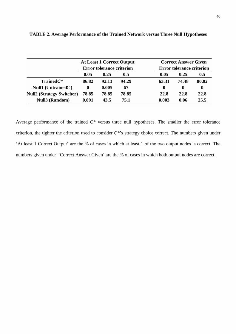
40

TABLE 2. Average Performance of the Trained Network versus Three Null Hypotheses

Average performance of the trained C* versus three null hypotheses. The smaller the error tolerance

criterion, the tighter the criterion used to consider C*’s strategy choice correct. The numbers given under

‘At least 1 Correct Output’ are the % of cases in which at least 1 of the two output nodes is correct. The

numbers given under ‘Correct Answer Given’ are the % of cases in which both output nodes are correct.

At Least 1 Correct Output Correct Answer GivenError tolerance criterion Error tolerance criterion0.05 0.25 0.5 0.05 0.25 0.5

Trained C* 86.82 92.13 94.29 63.31 74.48 80.02Null1 (Untrained C ) 0 0.005 67 0 0 0

Null2 (Strategy Switcher) 78.85 78.85 78.85 22.8 22.8 22.8Null3 (Random) 0.091 43.5 75.1 0.003 0.06 25.5

41

TABLE 3. Answerable Games and Relationship to Nash

Answerable games are games for which the Nash algorithm provides one, and exactly one, solution. The

percentage is equal to (Number of Answerable Games)/2000. The central column considers the cases

where these unique solutions coincide with the pure Nash equilibrium of the game. The right column

adjusts this Nash predictive success of the non Nash algorithm by making an auxiliary assumption on the

agent’s play in games where the non Nash algorithm does not provide a unique solution: namely, we

assume that the agent randomizes over all the choices (two or three, according to the game) admissible

according to the non Nash algorithm (e.g., in the case of rationalizability, all the non dominated solutions).

Non Nash Algorithm Answerable Uniquely predicted Expected performanceGames (%) Nash equilibria (%) in predicting Nash (%)

0 Level Strict Dominance 18.3 18.3 46.971 Level Strict Dominance 39.75 39.75 62.19Rationalizability 59.35 59.35 74.78Naïve 100 67 67L2 99.75 88.4 88.48Maximum Payoff Dominance 99.6 62.1 62.23Minmax 99.75 58.55 58.63Nearest Neighbor 100 62.8 62.8

42

TABLE 4. Describability of C*’s Behavior by Non Nash Algorithms

% of correct answers over answerable games = (number of correct answers) / (number of answerable

games). Answerable games are games for which the algorithm identifies a unique solution. % of correct

answers over full testing set = (number of correct answers) / (number of answerable games). Expected

performance over full testing set: % of correct answers over full testing set + adjustment due to the

assumption of randomization over admissible actions in non answerable games.

AlgorithmOver Answerable Games Over Full Testing Set

γγγγ=0.5 γγγγ=0.25 γγγγ=0.05 γγγγ=0.5 γγγγ=0.25 γγγγ=0.05 γγγγ=0.5 γγγγ=0.25 γγγγ=0.05

Nash 80.38 75.7 66.53 80.38 75.7 66.53 80.38 75.7 66.53L2 85.11 82.23 76.54 84.9 82.03 76.35 84.98 82.11 76.44Naïve 67.71 63.48 55.97 67.71 63.48 55.97 67.71 63.48 55.97Rationalizability 86.44 82.57 74.36 51.3 49.01 44.13 64.16 61.94 57.18Nearest Neighbor 62.97 58.78 51.48 62.97 58.78 51.48 62.97 58.78 51.48MPD 61.08 57.02 49.95 60.84 56.79 49.75 60.84 56.79 49.76Minmax 57.75 53.83 46.89 57.6 53.7 46.77 57.67 53.77 46.851SD 87.63 84 76.25 34.83 33.39 30.31 54.51 53.15 50.190SD 90.83 87.79 80.98 16.62 16.06 14.82 43.91 43.35 42.12

% of Correct Answers % of Correct Answers Expected PerformanceOver Full Testing Set

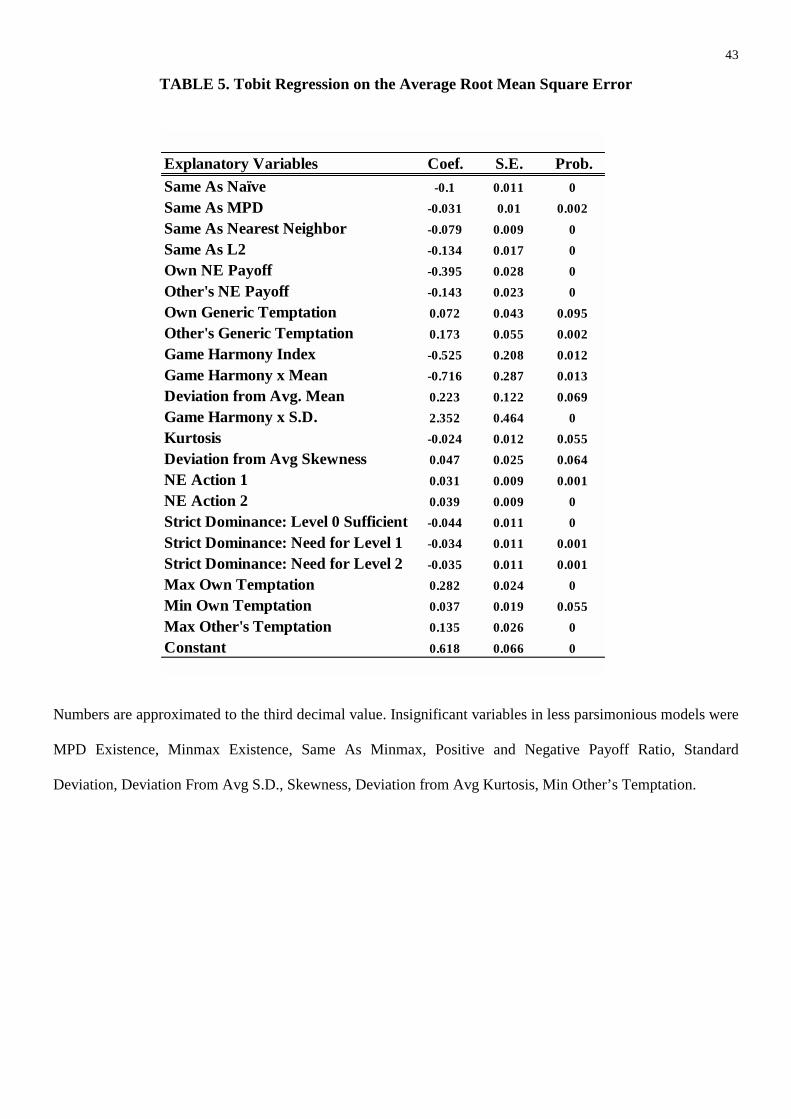
43

TABLE 5. Tobit Regression on the Average Root Mean Square Error

Numbers are approximated to the third decimal value. Insignificant variables in less parsimonious models were

MPD Existence, Minmax Existence, Same As Minmax, Positive and Negative Payoff Ratio, Standard

Deviation, Deviation From Avg S.D., Skewness, Deviation from Avg Kurtosis, Min Other’s Temptation.

Explanatory Variables Coef. S.E. Prob.Same As Naïve -0.1 0.011 0Same As MPD -0.031 0.01 0.002Same As Nearest Neighbor -0.079 0.009 0Same As L2 -0.134 0.017 0Own NE Payoff -0.395 0.028 0Other's NE Payoff -0.143 0.023 0Own Generic Temptation 0.072 0.043 0.095Other's Generic Temptation 0.173 0.055 0.002Game Harmony Index -0.525 0.208 0.012Game Harmony x Mean -0.716 0.287 0.013Deviation from Avg. Mean 0.223 0.122 0.069Game Harmony x S.D. 2.352 0.464 0Kurtosis -0.024 0.012 0.055Deviation from Avg Skewness 0.047 0.025 0.064NE Action 1 0.031 0.009 0.001NE Action 2 0.039 0.009 0Strict Dominance: Level 0 Sufficient -0.044 0.011 0Strict Dominance: Need for Level 1 -0.034 0.011 0.001Strict Dominance: Need for Level 2 -0.035 0.011 0.001Max Own Temptation 0.282 0.024 0Min Own Temptation 0.037 0.019 0.055Max Other's Temptation 0.135 0.026 0Constant 0.618 0.066 0

44

TABLE 6. Ordered Probit Regressions on NDecided1 and NDecided2, Games with Multiple PNE, n=5997

White robust estimators of the variance were used to compute standard errors. Numbers are approximated to

the third decimal value. Insignificant variables in less parsimonious models of both kinds were Same As 0SD,

Own’s BR Min Temptation, Game Harmony Index, Game Harmony x Other’s BR Temptation, Standard

Deviation, Game Harmony x S.D., Deviation From Avg S.D., Skewness, Deviation from Skewness, Kurtosis,

Deviation from Avg Kurtosis.

Explanatory NDecided1 NDecided2Variables Coef SE Prob Coef SE Prob

Same As Naïve 0.536 0.04 0 0.654 0.04 0Same As MPD 0.102 0.037 0.007Same As Minmax 0.087 0.038 0.021 0.101 0.036 0.005Same As 1SD 0.139 0.066 0.036Same As Utilitarian Best 0.186 0.043 0 0.226 0.043 0Same As L2 0.957 0.034 0 1.079 0.032 0Same As NE When 2NE 0.116 0.047 0.013Positive Payoff Ratio -0.067 0.023 0.004Negative Payoff Ratio 0.458 0.141 0.001Own BR Max Temptation -1.441 0.11 0 -1.705 0.113 0Other's BR Max Temptation -0.898 0.148 0 -1.007 0.145 0Other's BR Min Temptation -0.722 0.1 0 -0.91 0.096 0Own BR Payoff 2.568 0.167 0 2.543 0.09 0Other's BR Payoff 0.498 0.095 0Own Max Temptation -1.603 0.088 0 -2.491 0.283 0Other's Max Temptation -0.228 0.084 0.007 -0.573 0.082 0Own Min Temptation -0.527 0.096 0 -0.607 0.093 0Other's Min Temptation -0.661 0.087 0 -0.597 0.087 0Own Generic Temptation -2.04 0.306 0 -2.305 0.299 0Other's Generic Temptation -0.571 0.226 0.012 -0.384 0.219 0.079Game Harmony x Own BR Temptation 1.907 0.768 0.013Mean 6.47 0.583 0 7.667 0.629 0Game Harmony x Mean -1.449 0.887 0.102NE Action 1 -0.112 0.037 0.003 -0.109 0.036 0.003NE Action 2 -0.235 0.035 0 -0.159 0.034 0

45

TABLE 7. Ordered Probit Regressions on NDecided1, Games with a Unique (n=5993) and Zero

Pure Nash Equilibria (n=5983)

White robust estimators of the variance were used to compute standard errors. Numbers are approximated to

the third decimal value. Insignificant variables in less parsimonious models of both kinds were Same As

Minmax, Other’s BR Payoff, Game Harmony Index, Game Harmony x Other’s BR Temptation, Game

Harmony x Mean, Game Harmony x S.D., Deviation from Avg Mean, Deviation From Avg S.D., Skewness,

Deviation from Skewness, Kurtosis, Deviation from Avg Kurtosis.

Explanatory Unique Pure Nash Equilibrium Zero Pure Nash EquilibriaVariables Coef SE Prob Coef SE Prob

Same As NE 0.68 0.067 0Same As Naïve 0.556 0.043 0 0.685 0.035 0Same As MPD 0.254 0.039 0 0.536 0.033 0Same As 0SD -0.138 0.081 0.088Same As 1SD 0.124 0.063 0.048Same As L2 1.094 0.056 0 0.825 0.031 0Negative Payoff Ratio -0.439 0.138 0.001 0.669 0.157 0Own BR Max Temptation -1.547 0.096 0 -0.629 0.083 0Other's BR Max Temptation -0.877 0.159 0Own BR Min Temptation 0.174 0.09 0.053 -0.295 0.1 0.003Other's BR Min Temptation -0.285 0.101 0.005 0.238 0.073 0.001Own BR Payoff 2.12 0.294 0 2.447 0.194 0Own Max Temptation -0.266 0.073 0Other's Max Temptation -0.177 0.072 0.015Own Min Temptation 0.188 0.1 0.061 0.273 0.073 0Other's Min Temptation 0.24 0.063 0Own Generic Temptation -3.838 0.291 0 -1.49 0.199 0Other's Generic Temptation -1.059 0.195 0NE Action 1 -0.111 0.038 0.004 -0.307 0.034 0NE Action 2 -0.15 0.037 0 -0.224 0.033 0Game Harmony Index 1.74 0.438 0 1.538 0.243 0Game Harmony x Own BR Temptation -2.342 0.634 0Game Harmony x Other's BR Temptation -1.806 0.254 0Mean 6.119 0.55 0Standard Deviation 1.651 0.659 0.012

BOUNDED-RATIONAL BEHAVIOR BY NEURAL NETWORKS … · 2001-08-17 · BOUNDED-RATIONAL BEHAVIOR BY...

Documents

Transcript of BOUNDED-RATIONAL BEHAVIOR BY NEURAL NETWORKS … · 2001-08-17 · BOUNDED-RATIONAL BEHAVIOR BY...