Bounded var
37
Simplex algorithm for problems with bounded variables
-
Upload
samo-alwatan -
Category
Technology
-
view
76 -
download
1
Transcript of Bounded var
Simplex algorithm
for
problems with bounded variables
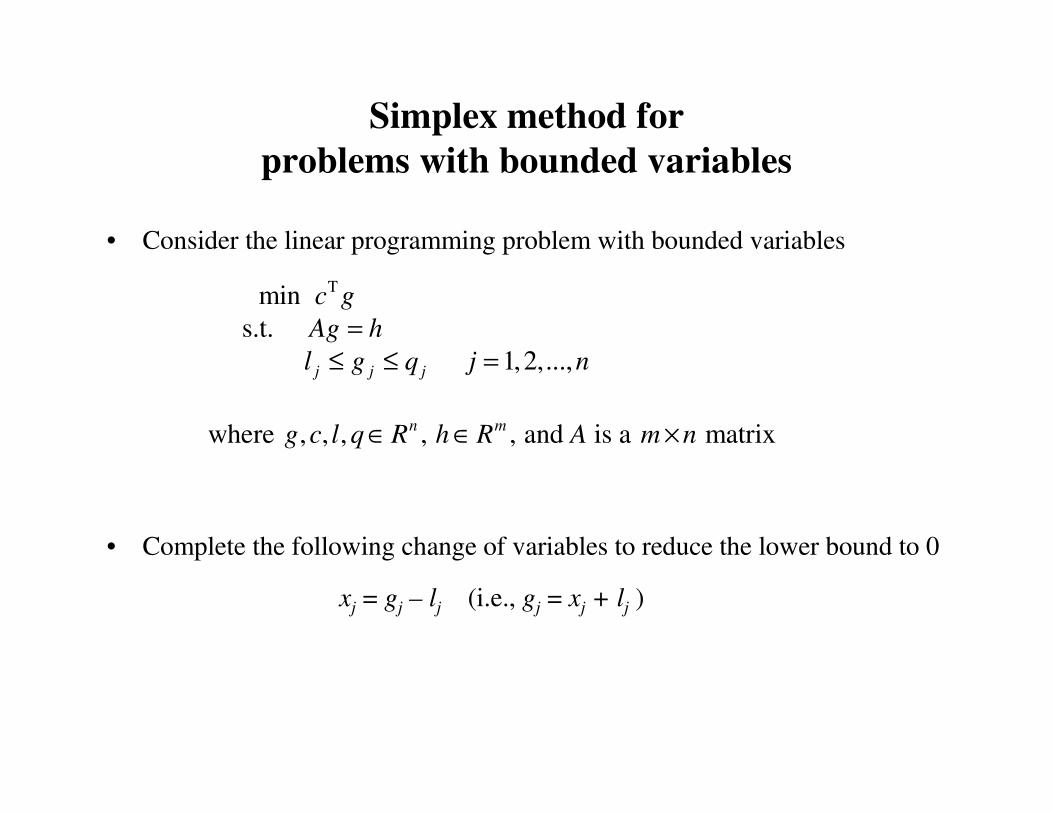
Simplex method for
problems with bounded variables
• Consider the linear programming problem with bounded variables
• Complete the following change of variables to reduce the lower bound to 0
xj = gj – lj (i.e., gj = xj + lj )
Tmin
s.t.
1,2,...,
where , , , , , and is a matrix
j j j
n m
c g
Ag h
l g q j n
g c l q R h R A m n
=
≤ ≤ =
∈ ∈ ×

Simplex method for
problems with bounded variables
the problem becomes
• Complete the following change of variables to reduce the lower bound to 0
xj = gj – lj (i.e., gj = xj + lj )
Tmin ( )
s.t. ( )
1,2,...,
where , , , , , and is a matrix
j j j j
n m
c x l
A x l h
l x l q j n
c x l q R h R A m n
+
+ =
≤ + ≤ =
∈ ∈ ×
Tmin
s.t.
1,2,...,j j j
c g
Ag h
l g q j n
=
≤ ≤ =

Simplex method for
problems with bounded variables
the problem becomes
replacing : uj = qj – lj and b = h – Al
T Tmin
s.t.
0 1,2,...,j j
c x c l
Ax b
x u j n
+
=
≤ ≤ =
Tmin ( )
s.t. ( )
1,2,...,
where , , , , , and is a matrix
j j j j
n m
c x l
A x l h
l x l q j n
c x l q R h R A m n
+
+ =
≤ + ≤ =
∈ ∈ ×
T Tmin
s.t.
1,2,...,j j j j j j j
c x c l
Ax h Al
l l x l l q l j n
+
= −
− ≤ + − ≤ − =

• In this problem
since cTl is a constant, we can eliminate it from the minimisation without
modifying the optimal solution.
Then in the rest of the presentation we consider the problem without this
constant.
Simplex method for
problems with bounded variables
T T Tmin
s.t.
0 1,2,...,j j
c l c x c l
Ax b
x u j n
+ +
=
≤ ≤ =
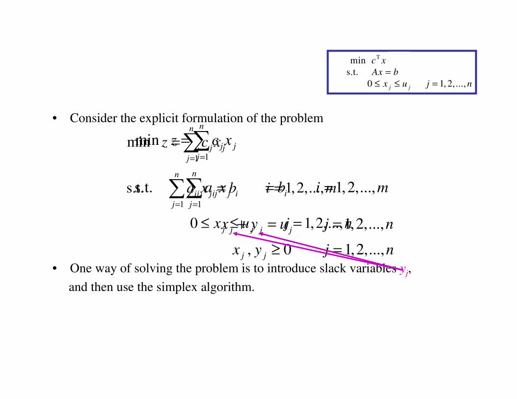
• Consider the explicit formulation of the problem
• One way of solving the problem is to introduce slack variables yj,
and then use the simplex algorithm.
1
1
min
s.t. 1,2,...,
0 1,2,...,
n
j j
j
n
ij j i
j
j j
z c x
a x b i m
x u j n
=
=
=
= =
≤ ≤ =
∑
∑
1
1
min
s.t. 1,2,...,
1,2,...,
, 0 1,2,...,
n
j j
j
n
ij j i
j
j j j
j j
z c x
a x b i m
x y u j n
x y j n
=
=
=
= =
+ = =
≥ =
∑
∑
T Tmin
s.t.
0 1, 2,...,j j
c x c l
Ax b
x u j n
+
=
≤ ≤ =

1
1
min
s.t. 1,2,...,
0 1,2,...,
n
j j
j
n
ij j i
j
j j
z c x
a x b i m
x u j n
=
=
=
= =
≤ ≤ =
∑
∑
1
1
min
s.t. 1,2,...,
1,2,...,
, 0 1,2,...,
n
j j
j
n
ij j i
j
j j j
j j
z c x
a x b i m
x y u j n
x y j n
=
=
=
= =
+ = =
≥ =
∑
∑
account implicitly
Tableau with rowsm n+
Tableau with rowsm

• Consider a basic feasible solution of this problem
• Because of the constraints xj + yj = uj, at least one of the variables xj or yj is
basic, j = 1,2,…,n.
• Then for all j = 1,2,…,n, one of the three situations holds:
a) xj = uj is basic and yj = 0 is non basic
b) xj = 0 is non basic and yj = uj is basic
c) 0 < xj < uj is basic and 0 < yj < uj is basic
1
1
min
s.t. 1,2,...,
1,2,...,
, 0 1,2,...,
n
j j
j
n
ij j i
j
j j j
j j
z c x
a x b i m
x y u j n
x y j n
=
=
=
= =
+ = =
≥ =
∑
∑Non degeneracy:
all the basic variables
are positive at
each iteration
njyx
njuyx
mibxa
xcz
jj
jjj
n
j
ijij
n
j
jj
,...,2,10,
,...,2,1
,...,2,1àSujet
min
1
1
=≥
==+
==
=
∑
∑
=
=
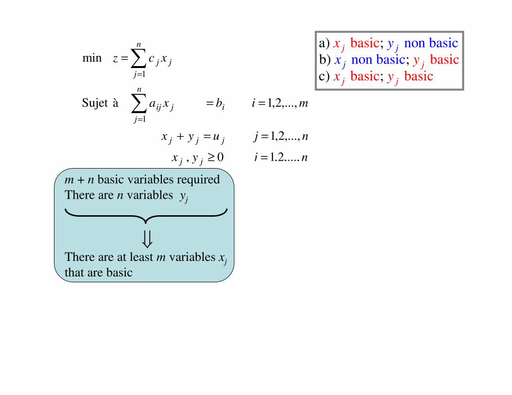
m + n basic variables required
There are n variables yj
There are at least m variables xj
that are basic
Exactly m variables xj satisfying
0 < xj < uj.
For contradiction, if m0 m variables xj
satisfy the relation, then the
m0 corresponding variables yj would be
basic.
Furthermore, for the n – m0 other indices j,
either xj = uj (case a) or yj = uj (case b)
would be verified.
Then the number of basic variables
would be equal to
2m0 + (n – m0) = m0 + n m + n
≠
≠
non basic
non basic
a) ;
b) ;
basic
basi
c)
c
basic b ; asic
j
j
j
j
j
j
x
y
x y
y
x
⇓

njyx
njuyx
mibxa
xcz
jj
jjj
n
j
ijij
n
j
jj
,...,2,10,
,...,2,1
,...,2,1àSujet
min
1
1
=≥
==+
==
=
∑
∑
=
=
m + n basic variables required
There are n variables yj
There are at least m variables xj
that are basic
Exactly m variables xj satisfying
0 < xj < uj.
For contradiction, if m0 m variables xj
satisfy the relation, then the
m0 corresponding variables yj would be
basic.
Furthermore, for the n – m0 other indices j,
either xj = uj (case a) or yj = uj (case b)
would be verified.
Then the number of basic variables
would be equal to
2m0 + (n – m0) = m0 + n m + n
≠
≠
non basic
non basic
a) ;
b) ;
basic
basi
c)
c
basic b ; asic
j
j
j
j
j
j
x
y
x y
y
x
⇓

La base a donc la forme suivante
0 < xj < uj 0 < yj < uj xj=uj yj=uj
1
1
min
s.t. 1,2,...,
1,2,...,
, 0 1,2,...,
n
j j
j
n
ij j i
j
j j j
j j
z c x
a x b i m
x y u j n
x y j n
=
=
=
= =
+ = =
≥ =
∑
∑
Tmin
s.t. 0
, 0
z c x
Ax y b
Ix Iy u
x y
=
+ =
+ =
≥
m
m
n
0AI I
To simplify notation, assume
the following basic variables:
0 1, ,
0 1, ,
1, ,
1, ,
i i
i i
i i
i i
x u i m
y u i m
x u i m m l
y u i m l m n
< < =
< < =
= = + +
= = + + +
…
…
…
…

Tmin
Sujet à 0
, 0
z c x
Ax y b
Ix Iy u
x y
=
+ =
+ =
≥
The basis has the following form
0 < xj < uj 0 < yj < uj xj=uj yj=uj
1
1
min
s.t. 1,2,...,
1,2,...,
, 0 1,2,...,
n
j j
j
n
ij j i
j
j j j
j j
z c x
a x b i m
x y u j n
x y j n
=
=
=
= =
+ = =
≥ =
∑
∑
m
m
n
0AI I
1 1
2
3
m m n m−
Tmin
s.t. 0
, 0
z c x
Ax y b
Ix Iy u
x y
=
+ =
+ =
≥
To simplify notation, assume
the following basic variables:
0 1, ,
0 1, ,
1, ,
1, ,
i i
i i
i i
i i
x u i m
y u i m
x u i m m l
y u i m l m n
< < =
< < =
= = + +
= = + + +
…
…
…
…

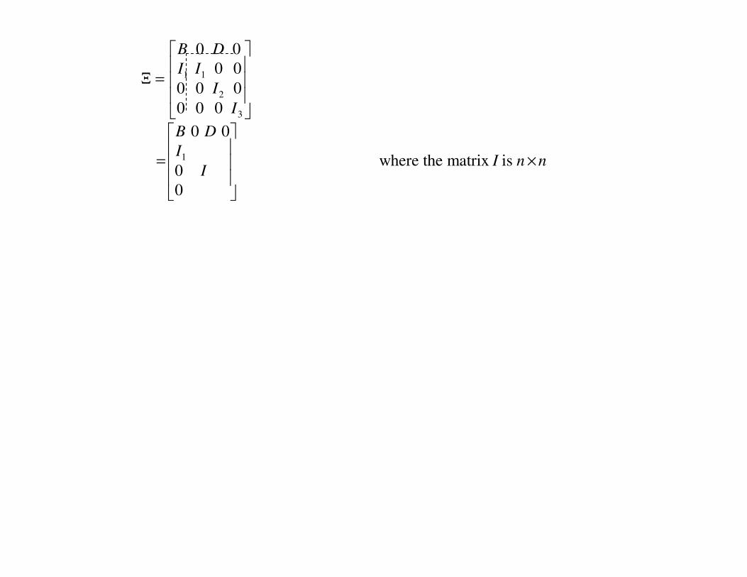
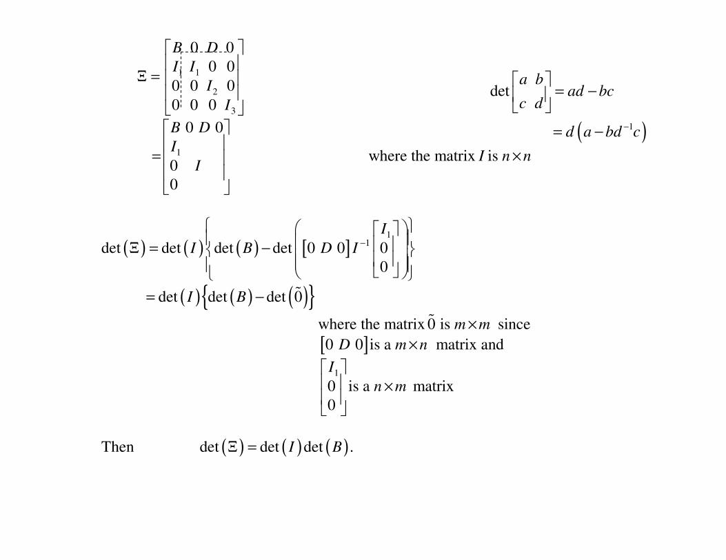
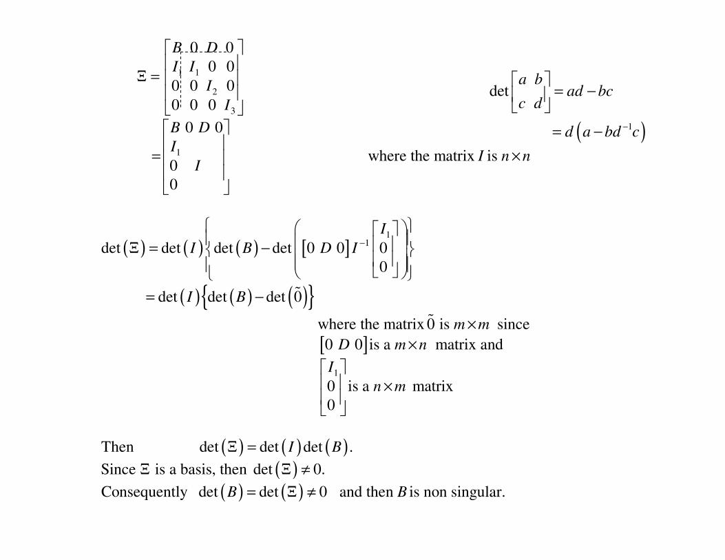
( ) ( ) ( ) [ ]
( ) ( ) ( ){ }
[ ]
1 1
2
3
1
11
1
0 0
0 0
0 0 0
0 0 0
0 0
where the matrix is 0
0
det det det det 0 0 0
0
det det det 0
where the matrix 0 is since
0 0 is a matrix and
0
0
B D
I I
I
I
B D
II n n
I
I
I B D I
I B
m m
D m n
I
−
Ξ =
= ×
Ξ = −
= −
×
×
�
�
( ) ( ) ( )( )
( ) ( )
is a matrix
Then det det det .
Since is a basis, then det 0.
Consequently det det 0 and then is non singular.
Then is a basis of .
n m
I B
B B
B A
×
Ξ =
Ξ Ξ ≠
= Ξ ≠
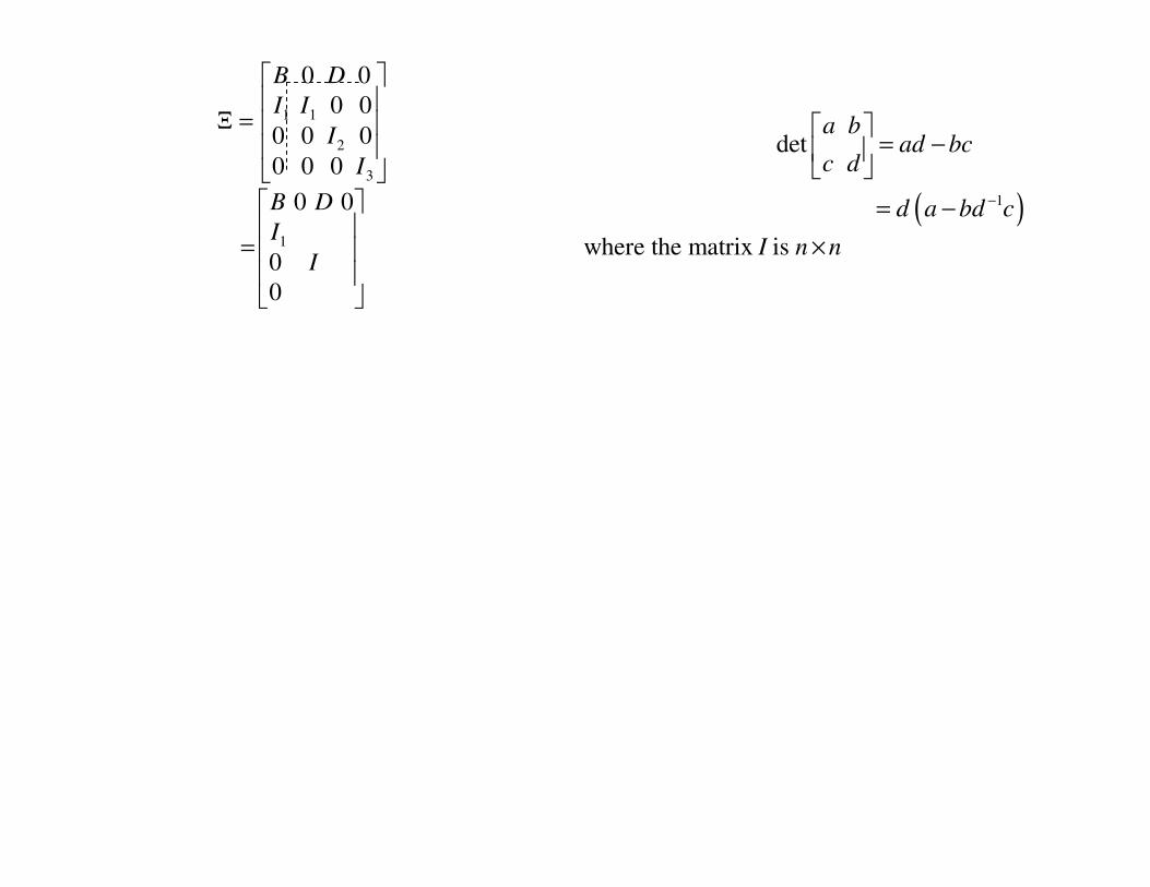
( )1
deta b
ad bcc d
d a bd c−
= −
= −

( ) ( ) ( ) [ ]
( ) ( ) ( ){ }
[ ]
1 1
2
3
1
11
1
0 0
0 0
0 0 0
0 0 0
0 0
where the matrix is 0
0
det det det det 0 0 0
0
det det det 0
where the matrix 0 is since
0 0 is a matrix and
0
0
B D
I I
I
I
B D
II n n
I
I
I B D I
I B
m m
D m n
I
−
Ξ =
= ×
Ξ = −
= −
×
×
�
�
( ) ( ) ( )( )
( ) ( )
is a matrix
Then det det det .
Since is a basis, then det 0.
Consequently det det 0 and then is non singular.
Then is a basis of .
n m
I B
B B
B A
×
Ξ =
Ξ Ξ ≠
= Ξ ≠
( )1
deta b
ad bcc d
d a bd c−
= −
= −
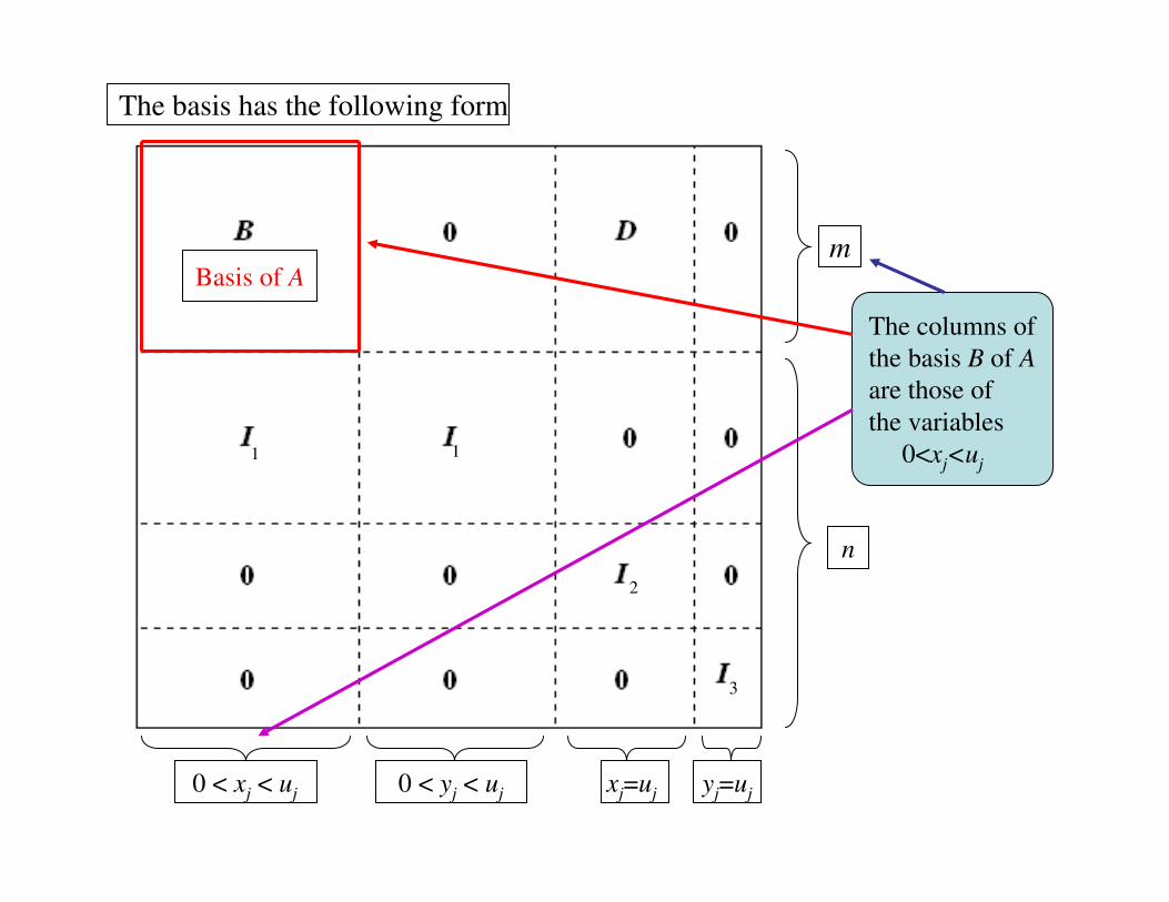
The basis has the following form
m
n
0 < xj < uj 0 < yj < uj xj=uj yj=uj
Basis of A
The columns of
the basis B of A
are those of
the variables
0<xj<uj1 1
2
3
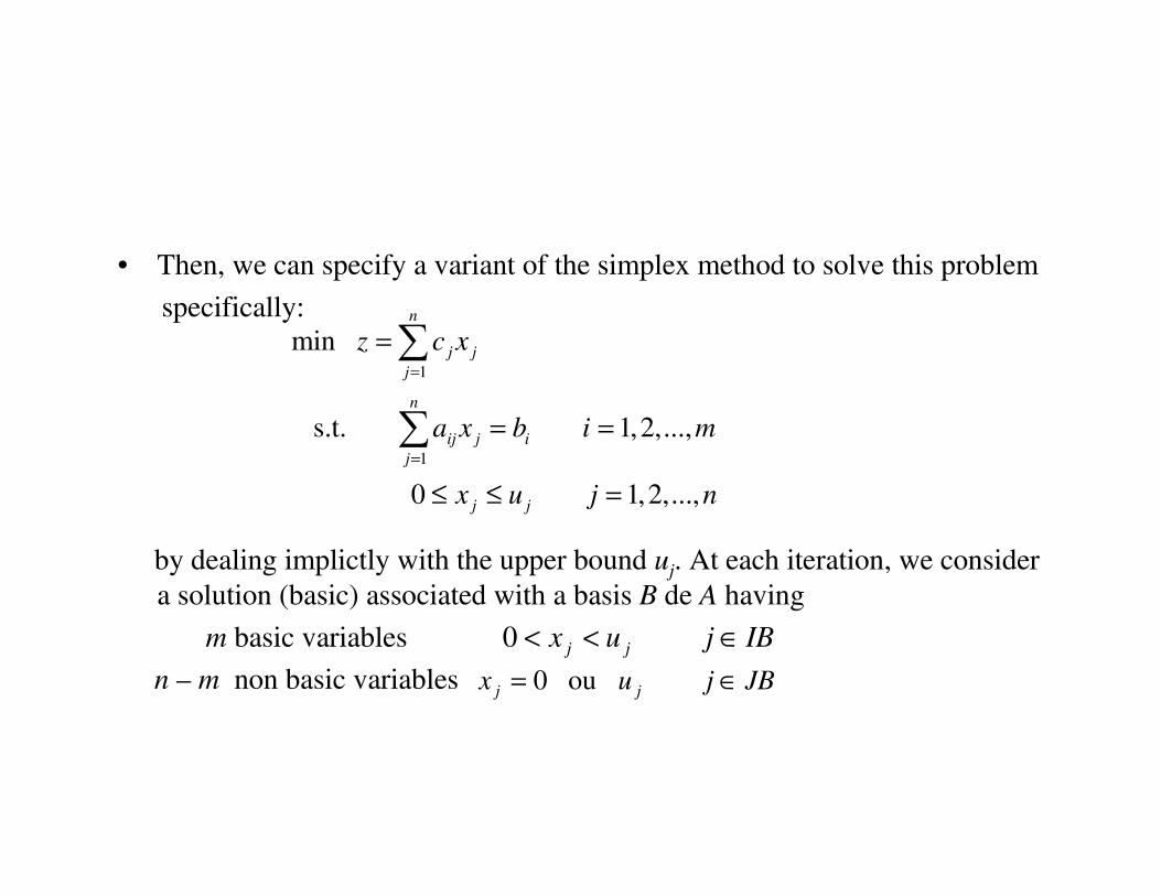
• Then, we can specify a variant of the simplex method to solve this problem
specifically:
by dealing implictly with the upper bound uj. At each iteration, we consider
a solution (basic) associated with a basis B de A having
m basic variables
n – m non basic variables
1
1
min
s.t. 1,2,...,
0 1,2,...,
n
j j
j
n
ij j i
j
j j
z c x
a x b i m
x u j n
=
=
=
= =
≤ ≤ =
∑
∑
JBjux jj ∈= ou0
IBjux jj ∈<<0
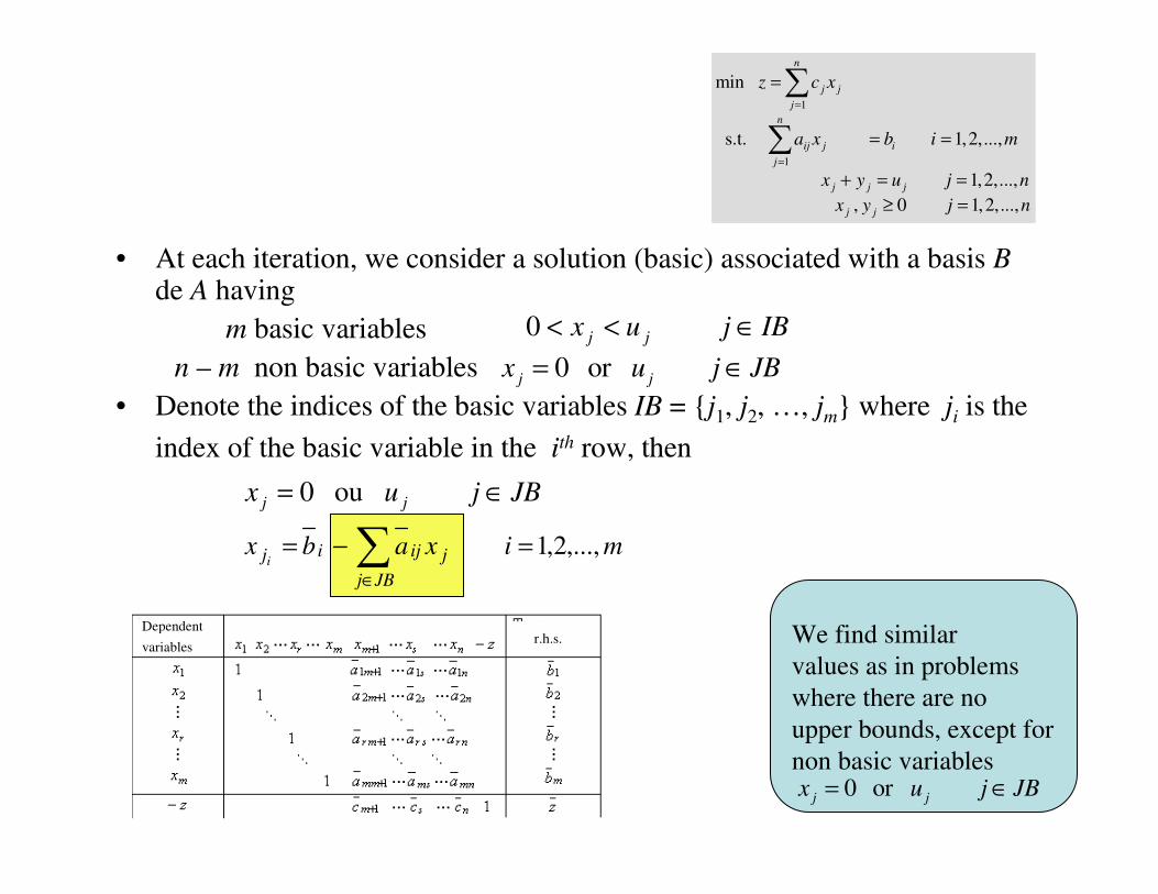
mixabx
JBj
jijiji,...,2,1=−= ∑
∈
• At each iteration, we consider a solution (basic) associated with a basis Bde A having
m basic variables
n – m non basic variables
• Denote the indices of the basic variables IB = {j1, j2, …, jm} where ji is the
index of the basic variable in the ith row, then
We find similar
values as in problems
where there are no
upper bounds, except for
non basic variables
IBjux jj ∈<<0
0 orj j
x u j JB= ∈
0 orj jx u j JB= ∈
1
1
min
s.t. 1,2,...,
1,2,...,
, 0 1,2,...,
n
j j
j
n
ij j i
j
j j j
j j
z c x
a x b i m
x y u j n
x y j n
=
=
=
= =
+ = =
≥ =
∑
∑
Dependent
variables r.h.s.
JBjux jj ∈= ou0
mixabx
JBj
jijiji,...,2,1=−= ∑
∈
We have to modify the entering criterion
and the leaving criterion accordingly to
generate a variant of the simplex algorithm
for this problem
We find similar
values as in problems
where there are no
upper bounds, except for
non basic variables
0 orj jx u j JB= ∈

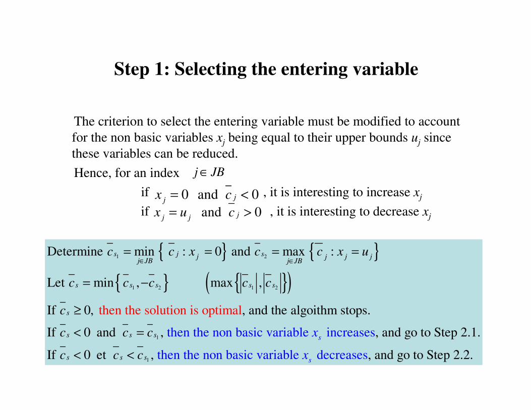
Step 1: Selecting the entering variable
The criterion to select the entering variable must be modified to account
for the non basic variables xj being equal to their upper bounds uj since
these variables can be reduced.
Hence, for an index
if , it is interesting to increase xj
if , it is interesting to decrease xj
JBj ∈
0 and 0jjx c= <
and 0jj jx u c= >
{ } { }
{ } { }( )
1 2
1 2 1 2
1
then the solution is optimal
Determine min : 0 and max :
Let min , max ,
If 0, , and the algoithm stops.
If 0 an then the non basic variable increasesd ,
s j sj j jjj JB j JB
s s s s s
s
s s ss
c c x c c x u
c c c c c
c
c c c x
∈ ∈= = = =
= −
≥
< =
1then the non basic variab
, and go to Step 2.1.
If le decre 0 et , , and go to Stases ep 2.2.s s s sxc c c< <
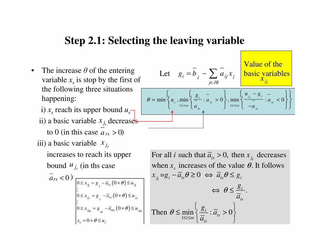
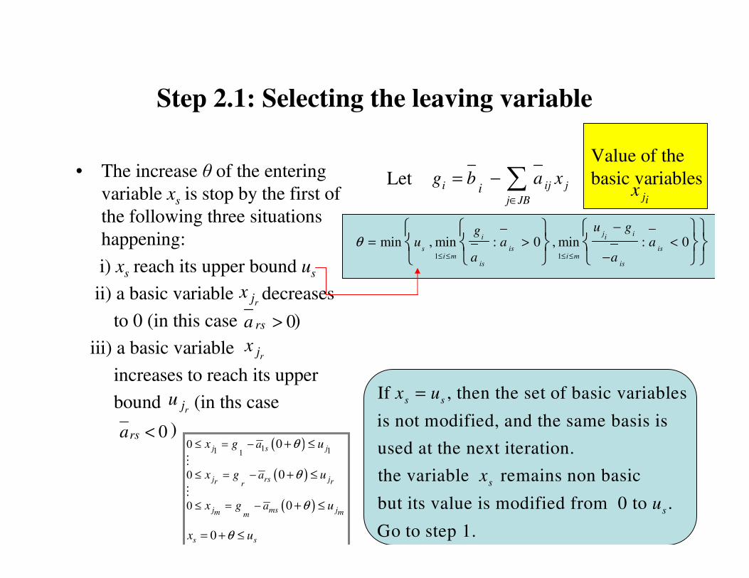
Step 2.1: Selecting the leaving variable
• The increase θ of the entering
variable xs is stop by the first of
the following three situations
happening:
i) xs reach its upper bound us
ii) a basic variable decreases
to 0 (in this case )
iii) a basic variable
increases to reach its upper
bound (in ths case
)
Let
rjx
0>rsa
rjx
rju
0rsa <
1 1
min , min : 0 , min : 0j ii i
is issi m i m
is is
u ggu a a
a aθ
≤ ≤ ≤ ≤
−
= > <
−
iji j
j JBi
g b a x∈
= − ∑Value of the
basic variables ij
x
1
For all such that 0, then decreases
when increases of the value . It follows
= 0
.
Then min : 0
is ji
s
j i is is ii
i
is
iis
i mis
i a x
x
x g a a g
g
a
ga
a
θ
θ θ
θ
θ≤ ≤
>
− ≥ ⇔ ≤
⇔ ≤
≤ >
( )
( )
( )
11 110
0
0
0
0
0
0
j s j
j rs jr rr
j ms jm mm
s s
a
a
a
x g u
x g u
x g u
x u
θ
θ
θ
θ
≤ = −
≤ = −
≤ = −
+ ≤
+ ≤
+ ≤
= + ≤
�
�

Step 2.1: Selecting the leaving variable
• The increase θ of the entering
variable xs is stop by the first of
the following three situations
happening:
i) xs reach its upper bound us
ii) a basic variable decreases
to 0 (in this case )
iii) a basic variable
increases to reach its upper
bound (in ths case
)
Let
rjx
0>rsa
rjx
rju
0rsa <
1 1
min , min : 0 , min : 0j ii i
is issi m i m
is is
u ggu a a
a aθ
≤ ≤ ≤ ≤
−
= > <
−
iji j
j JBi
g b a x∈
= − ∑
Si θ = ∞, alors le problème n’est pas
borné inférieurement et l’algorithme
s’arrête.
Value of the
basic variables ij
x
1
For all such that 0, then increses
when increases of the value . It follows
=
.
Then min : 0
is ji
s
j i is j is j ii i i
j ii
is
j iiis
i mis
i a x
x
x g a u a u g
u g
a
u ga
a
θ
θ θ
θ
θ≤ ≤
<
− ≤ ⇔ − ≤ −
−⇔ ≤
−
− ≤ <
−
( )
( )
( )
11 110
0
0
0
0
0
0
j s j
j rs jr rr
j ms jm mm
s s
a
a
a
x g u
x g u
x g u
x u
θ
θ
θ
θ
≤ = −
≤ = −
≤ = −
+ ≤
+ ≤
+ ≤
= + ≤
�
�
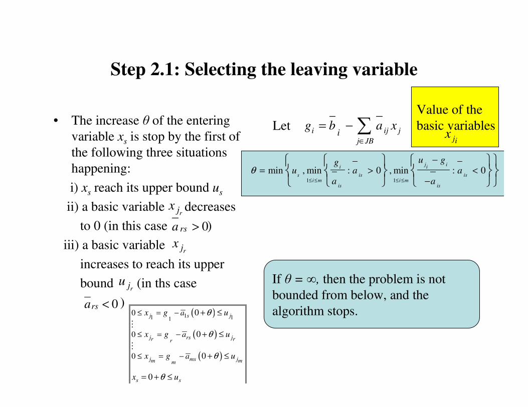
Step 2.1: Selecting the leaving variable
• The increase θ of the entering
variable xs is stop by the first of
the following three situations
happening:
i) xs reach its upper bound us
ii) a basic variable decreases
to 0 (in this case )
iii) a basic variable
increases to reach its upper
bound (in ths case
)
Let
rjx
0>rsa
rjx
rju
0rsa <
1 1
min , min : 0 , min : 0j ii i
is issi m i m
is is
u ggu a a
a aθ
≤ ≤ ≤ ≤
−
= > <
−
iji j
j JBi
g b a x∈
= − ∑
If θ = ∞, then the problem is not
bounded from below, and the
algorithm stops.
Value of the
basic variables ij
x
( )
( )
( )
11 110
0
0
0
0
0
0
j s j
j rs jr rr
j ms jm mm
s s
a
a
a
x g u
x g u
x g u
x u
θ
θ
θ
θ
≤ = −
≤ = −
≤ = −
+ ≤
+ ≤
+ ≤
= + ≤
�
�
Step 2.1: Selecting the leaving variable
• The increase θ of the entering
variable xs is stop by the first of
the following three situations
happening:
i) xs reach its upper bound us
ii) a basic variable decreases
to 0 (in this case )
iii) a basic variable
increases to reach its upper
bound (in ths case
)
Let
rjx
0>rsa
rjx
rju
0rsa <
1 1
min , min : 0 , min : 0j ii i
is issi m i m
is is
u ggu a a
a aθ
≤ ≤ ≤ ≤
−
= > <
−
iji j
j JBi
g b a x∈
= − ∑Value of the
basic variables ij
x
( )
( )
( )
11 110
0
0
0
0
0
0
j s j
j rs jr rr
j ms jm mm
s s
a
a
a
x g u
x g u
x g u
x u
θ
θ
θ
θ
≤ = −
≤ = −
≤ = −
+ ≤
+ ≤
+ ≤
= + ≤
�
�
If , then the set of basic variables
is not modified, and the same basis is
used at the next iteration.
the variable remains non basic
but its value is modified from 0 to .
Go to step 1.
s s
s
s
x u
x
u
=

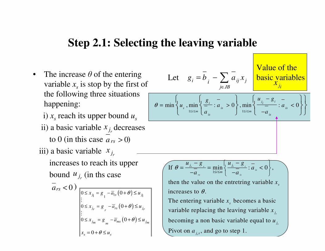
Step 2.1: Selecting the leaving variable
• The increase θ of the entering
variable xs is stop by the first of
the following three situations
happening:
i) xs reach its upper bound us
ii) a basic variable decreases
to 0 (in this case )
iii) a basic variable
increases to reach its upper
bound (in ths case
)
Let
rjx
0>rsa
rjx
rju
0rsa <
1 1
min , min : 0 , min : 0j ii i
is issi m i m
is is
u ggu a a
a aθ
≤ ≤ ≤ ≤
−
= > <
−
iji j
j JBi
g b a x∈
= − ∑Value of the
basic variables ij
x
( )
( )
( )
11 110
0
0
0
0
0
0
j s j
j rs jr rr
j ms jm mm
s s
a
a
a
x g u
x g u
x g u
x u
θ
θ
θ
θ
≤ = −
≤ = −
≤ = −
+ ≤
+ ≤
+ ≤
= + ≤
�
�
1If min : 0 ,
then the value on the entretring variable
increases to .
The entering variable becomes a basic
variable replacing the leaving variable
becoming a non basic
ir
is
rs is
r
i m
s
s
j
gga
a a
x
x
x
θ
θ
≤ ≤
= = >
variable equal to 0
Pivot on , and go to step 1.rj s
a
Step 2.1: Selecting the leaving variable
• The increase θ of the entering
variable xs is stop by the first of
the following three situations
happening:
i) xs reach its upper bound us
ii) a basic variable decreases
to 0 (in this case )
iii) a basic variable
increases to reach its upper
bound (in ths case
)
Let
rjx
0>rsa
rjx
rju
0rsa <
1 1
min , min : 0 , min : 0j ii i
is issi m i m
is is
u ggu a a
a aθ
≤ ≤ ≤ ≤
−
= > <
−
iji j
j JBi
g b a x∈
= − ∑Value of the
basic variables ij
x
( )
( )
( )
11 110
0
0
0
0
0
0
j s j
j rs jr rr
j ms jm mm
s s
a
a
a
x g u
x g u
x g u
x u
θ
θ
θ
θ
≤ = −
≤ = −
≤ = −
+ ≤
+ ≤
+ ≤
= + ≤
�
�
1If min : 0 ,
then the value on the entretring variable
increases to .
The entering variable becomes a basic
variable replacing the leaving variable
becoming a
i ir r
is
rs is
r
jj
i m
s
s
j
u gu ga
a a
x
x
x
θ
θ
≤ ≤
−− = = <
− −
non basic variable equal to
Pivot on , and go to step 1.
r
r
j
j s
u
a
Step 1: Selecting the entering variable
The criterion to select the entering variable must be modified to account
for the non basic variables xj being equal to their upper bounds uj since
these variables can be reduced.
Hence, for an index
if , it is interesting to increase xj
if , it is interesting to decrease xj
JBj ∈
0 and 0jjx c= <
and 0jj jx u c= >
{ } { }
{ } { }( )
1 2
1 2 1 2
1
then the solution is optimal
Determine min : 0 and max :
Let min , max ,
If 0, , and the algoithm stops.
If 0 an then the non basic variable increasesd ,
s j sj j jjj JB j JB
s s s s s
s
s s ss
c c x c c x u
c c c c c
c
c c c x
∈ ∈= = = =
= −
≥
< =
1then the non basic variab
, and go to Step 2.1.
If le decre 0 et , , and go to Stases ep 2.2.s s s sxc c c< <

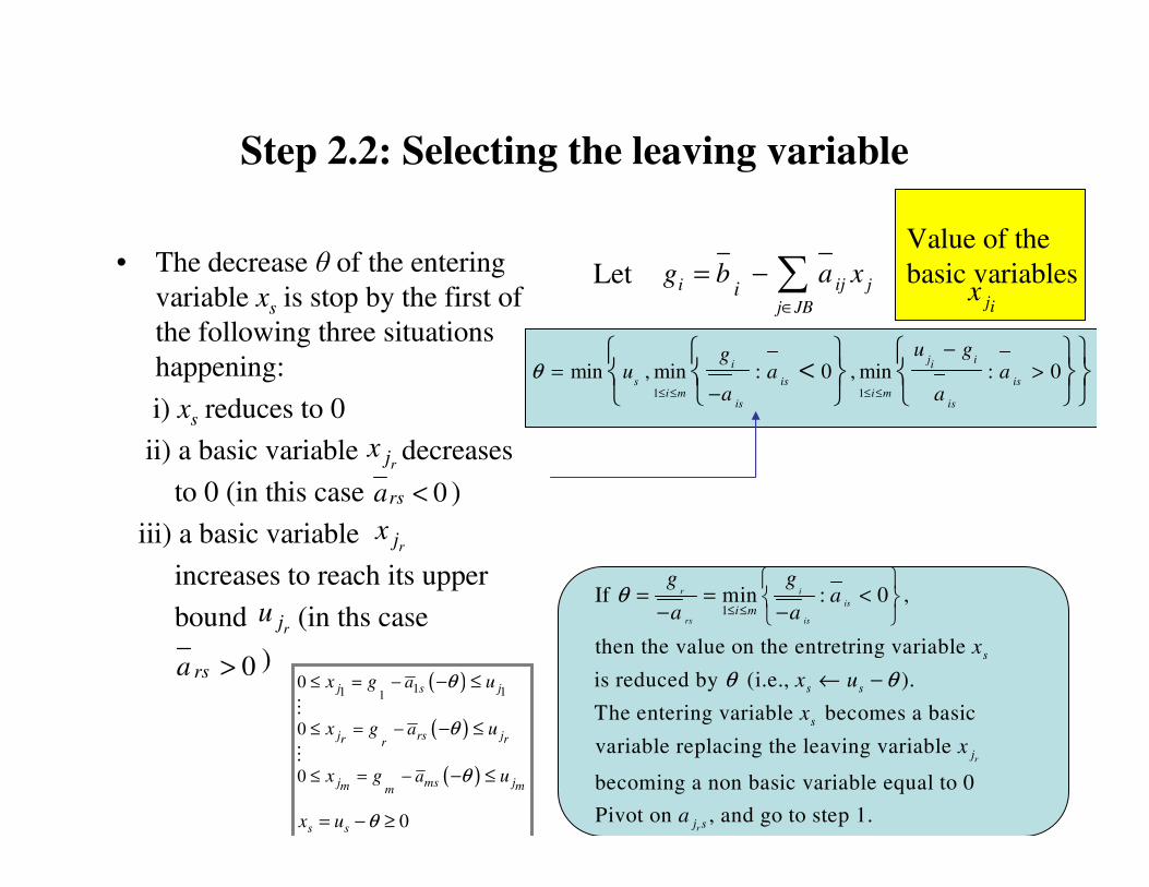
Step 2.2: Selecting the leaving variable
• The decrease θ of the entering
variable xs is stop by the first of
the following three situations
happening:
i) xs reduces to 0
ii) a basic variable decreases
to 0 (in this case )
iii) a basic variable
increases to reach its upper
bound (in this case
)
Let
rjx
0>rsa
rjx
rju
0rsa <
1 1
min , min : 0 , min : 0j ii i
is issi m i m
is is
u ggu a a
a aθ
≤ ≤ ≤ ≤
−= >
−
<
iji j
j JBi
g b a x∈
= − ∑Value of the
basic variables ij
x
( )
1
For all such that 0, then decreases
when decreases of the value . It follows
= 0
.
Then min : 0
is ji
s
j i is is ii
i
is
iis
i mis
i a x
x
x g a a g
g
a
ga
a
θ
θ θ
θ
θ≤ ≤
<
− − ≥ ⇔ − ≤
⇔ ≤−
≤ <
−
( )
( )
( )
11 110
0
0
0
j s j
j rs jr rr
j ms jm mm
s s
a
a
a
x g u
x g u
x g u
x u
θ
θ
θ
θ
≤ = −
≤ = −
≤ = −
− ≤
− ≤
− ≤
= − ≥
�
�

Step 2.2: Selecting the leaving variable
• The decrease θ of the entering
variable xs is stop by the first of
the following three situations
happening:
i) xs reduces to 0
ii) a basic variable decreases
to 0 (in this case )
iii) a basic variable
increases to reach its upper
bound (in ths case
)
Let
rjx
0>rsa
rjx
rju
0rsa <
1 1
min , min : 0 , min : 0j ii i
is issi m i m
is is
u ggu a a
a aθ
≤ ≤ ≤ ≤
−= >
−
<
iji j
j JBi
g b a x∈
= − ∑Value of the
basic variables ij
x
( )
1
For all such that 0, then increases
when decreasess of the value . It follows
=
.
Then min : 0
is ji
s
j i is j is j ii i i
j ii
is
j iiis
i mis
i a x
x
x g a u a u g
u g
a
u ga
a
θ
θ θ
θ
θ≤ ≤
>
− − ≤ ⇔ ≤ −
−⇔ ≤
− ≤ >
( )
( )
( )
11 110
0
0
0
j s j
j rs jr rr
j ms jm mm
s s
a
a
a
x g u
x g u
x g u
x u
θ
θ
θ
θ
≤ = −
≤ = −
≤ = −
− ≤
− ≤
− ≤
= − ≥
�
�

Step 2.2: Selecting the leaving variable
• The decrease θ of the entering
variable xs is stop by the first of
the following three situations
happening:
i) xs reduces to 0
ii) a basic variable decreases
to 0 (in this case )
iii) a basic variable
increases to reach its upper
bound (in ths case
)
Let
rjx
0>rsa
rjx
rju
0rsa <
1 1
min , min : 0 , min : 0j ii i
is issi m i m
is is
u ggu a a
a aθ
≤ ≤ ≤ ≤
−= >
−
<
iji j
j JBi
g b a x∈
= − ∑Value of the
basic variables ij
x
( )
( )
( )
11 110
0
0
0
j s j
j rs jr rr
j ms jm mm
s s
a
a
a
x g u
x g u
x g u
x u
θ
θ
θ
θ
≤ = −
≤ = −
≤ = −
− ≤
− ≤
− ≤
= − ≥
�
�
If , then the set of basic variables
is not modified, and the same basis is
used at the next iteration.
the variable remains non basic
but its value is modified from to 0.
Go to step 1.
s
s
s
u
x
u
θ =
Step 2.2: Selecting the leaving variable
• The decrease θ of the entering
variable xs is stop by the first of
the following three situations
happening:
i) xs reduces to 0
ii) a basic variable decreases
to 0 (in this case )
iii) a basic variable
increases to reach its upper
bound (in ths case
)
Let
rjx
0>rsa
rjx
rju
0rsa <
1 1
min , min : 0 , min : 0j ii i
is issi m i m
is is
u ggu a a
a aθ
≤ ≤ ≤ ≤
−= >
−
<
iji j
j JBi
g b a x∈
= − ∑Value of the
basic variables ij
x
( )
( )
( )
11 110
0
0
0
j s j
j rs jr rr
j ms jm mm
s s
a
a
a
x g u
x g u
x g u
x u
θ
θ
θ
θ
≤ = −
≤ = −
≤ = −
− ≤
− ≤
− ≤
= − ≥
�
�
1If min : 0 ,
then the value on the entretring variable
is reduced by (i.e., ).
The entering variable becomes a basic
variable replacing the leaving variable
b
ir
is
rs is
r
i m
s
s s
s
j
gga
a a
x
x u
x
x
θ
θ θ
≤ ≤
= = <
− −
← −
ecoming a non basic variable equal to 0
Pivot on , and go to step 1.rj s
a

Step 2.2: Selecting the leaving variable
• The decrease θ of the entering
variable xs is stop by the first of
the following three situations
happening:
i) xs reduces to 0
ii) a basic variable decreases
to 0 (in this case )
iii) a basic variable
increases to reach its upper
bound (in ths case
)
Let
rjx
0>rsa
rjx
rju
0rsa <
1 1
min , min : 0 , min : 0j ii i
is issi m i m
is is
u ggu a a
a aθ
≤ ≤ ≤ ≤
−= >
−
<
iji j
j JBi
g b a x∈
= − ∑Value of the
basic variables ij
x
( )
( )
( )
11 110
0
0
0
j s j
j rs jr rr
j ms jm mm
s s
a
a
a
x g u
x g u
x g u
x u
θ
θ
θ
θ
≤ = −
≤ = −
≤ = −
− ≤
− ≤
− ≤
= − ≥
�
�
1If min : 0 ,
then the value on the entretring variable
is reduced by (i.e., ).
The entering variable becomes a basic
variable replacing the leaving variabl
i ir r
is
rs is
jj
i m
s
s s
s
u gu ga
a a
x
x u
x
θ
θ θ
≤ ≤
−− = = >
← −
e
becoming a non basic variable equal to
Pivot on , and go to step 1.
r
r
r
j
j
j s
x
u
a

References
M.S. Bazaraa, J.J. Jarvis, H.D. Sherali, “ Linear Programming and Network Flows”, 3rd edition, Wiley-Interscience (2005), p. 217
F.S. Hillier, G.J. Lieberman, “Introduction to Operations Research”, Mc GrawHill (2005), Section 7.3
D. G. Luenberger, “ Linear and Nonlinear Programming ”, 2nd edition, Addison-Wesley (1984), Section 3.6