Applied Economics and Finance

Vol. 5, No. 3; May 2018

ISSN 2332-7294 E-ISSN 2332-7308

Published by Redfame Publishing

URL: http://aef.redfame.com

49

Bollinger Bands Trading Strategy Based on Wavelet Analysis

Shaozhen Chen1, Bangqian Zhang1, Gengjian Zhou1 & Qiaoxu Qin1

1Finance Department of International Bussiness School, Jinan University, Zhuhai, Guangdong Province, China

Correspondence: Qiaoxu Qin, Finance Department of International Business School, Jinan University, Qianshan Road

206#, Zhuhai City, Guangdong Province, Post No. 519070, China.

Received: March 6, 2018 Accepted: March 26, 2018 Available online: April 2, 2018

doi:10.11114/aef.v5i3.3079 URL: https://doi.org/10.11114/aef.v5i3.3079

Abstract

With the popularization of the concept of quantitative investment and the introduction of stock index futures in China,

the research on the quantitative trading strategies of stock index futures is emerging gradually. This paper takes the CSI

300 stock index futures as the research object and sets up the Bollinger Bands trading strategy to test it, while

considering the factors such as returns, retracement and income risk ratio, etc. Furthermore, the paper uses the wavelet

noise reduction to process the data of price and the Bollinger Bands trading strategy to test the processed data.

Compared with the results of the first test, the Bollinger Band trading strategy based on wavelet analysis has greater

returns, less risk and better applicability.

Keywords: Bollinger Bands trading strategy, wavelet analysis

1. Introduction

Quantitative transaction means using the computer software and mathematical model to practice investment philosophy

and achieve the investment strategy. Its advantages lie in discipline, system, timeliness, accuracy and decentralization.

With the continuous popularization of the concept of quantitative investment in China and the introduction of CSI 300

index futures launched by China Financial Futures on April 16, 2010, the quantitative trading operation of CSI 300

stock index futures in Chinese stock market has become increasingly popular.

Quantitative timing is a form of quantitative transactions, which uses quantitative methods to analyze various macro and

micro indicators and find the key information that affects the market trend and forecasts the future trend. Quantitative

timing strategy has many research perspectives, the most common of which is the trend timing. Madhavan (2002)

proposed the VMA strategy, which has the function of price forecasting, mean reversion and trending tracker. The test

showed the strategy could achieve greater profit. Wongsasutthikul (2012) built a “Hurst Trading” strategy based on

Hurst exponent. The empirical reasearch showed that during the period between 2002 and 2011, the Hurst Trading

strategy was able to outperform the traditional momentum strategy and the “Buy and Hold” strategy by a wide margin

on stock trading in the DJIA Index, SPX Index, and R2500 Index. Su (2015) developed PCA-SVM quantitative timing

strategy based on SVM model. The empirical results showed that the PCA-SVM strategy had greater stability and

higher profitability. Li (2016) focused on the trending strategies of the MA, the MACD, the DMA, and the TRIX.

Through the simulation test, the strategies all could obtain a good yield in the CSI 300 stock index futures market. Xie

(2016) built an improved R-Breaker strategy based on wavelet analysis and the strategy has a good return.

As the technical analysis indicators adopted for quantitative trading are based on the time series of stock index futures

(non-sationary time series), the use of the traditional time series model to process some non-stationary time series may

cause serious distortion, resulting in the occurrence of “false break” phenomenon (the misjudgment of trading point).

Therefore, the investors need to adjust the parameters and optimization to reduce the frequency of “false break”. The

wavelet analysis proposed by Grossman et al. (1984) could clearly reveal kinds of change periods hidden in the time

series, fully reflect the changing trend of the system in different time scales and evaluate the development trend of the

system qualitatively. As a result, the method of wavelet filtering could be combined with the existing quantitative

trading strategy to improve the accuracy of the trading. At present, about the research of wavelet denoising, the

domestic and foreign scholars mainly focus on the improvement and application of wavelet denoising algorithm.

Gençay et al. (2002) combined the neural network with wavelet denoising to construct a dynamic architecture and

proposed a test problem that can perform wavelet execution with multi-resolution. Edward et al. (2012) proposed a local

linear scale approximation (LLSA) algorithm based on the linear maximum overlap discrete wavelet transform

brought to you by COREView metadata, citation and similar papers at core.ac.uk

provided by Redfame Publishing: E-Journals

Applied Economics and Finance Vol. 5, No. 3; 2018

50

(MODWT), which made the denoising analysis suitable for high-frequency data mining. Liu et al. (2017) developed an

algorithm that could automatically correct the threshold according to the wavelet coefficient distribution of truncated

residuals, which enabled the wavelet threshold method to increase the wavelet denoising intensity without affecting the

signal.

In summary, the wavelet analysis is rarely applied in timing strategy. Therefore, this paper is trying to establish an

improved timing strategy based on wavelet analysis. Firstly, this paper takes the CSI 300 stock index futures as the

research object and sets up the Bollinger Bands trading strategy to test it, while considering the factors such as return,

retracement and income risk ratio, etc. Secondly, the paper uses the wavelet noise reduction to process the data of price

and the Bollinger Bands trading strategy to test the processed data. By comparing the results of the two tests, a more

robust trading strategy could be established, which has lower risk and higher returns. And the result of the research

could provide the investors with a new idea.

2. Theoretical Model

2.1 Bollinger Bands

Boiling Bands consist of three lines: the upper track, the middle track and the lower track;

The middle track = the average of the last n columns of closing prices of the underlying sequence;

The upper track = the middle track + k * the standard deviation of the closing price of the last n columns;

The lower track = the middle track–k * the standard deviation of the closing price of the last n columns;

Where k is a coefficient. Bollinger Bands can indicate support and stress positions, which can show both overbought

and oversold conditions and indicate the formation of a trend. When the selected k is large, the bandwidth of the

Bollinger Bands is large. If the stock price breaks the Bollinger’s upper track, we consider the market is overbought and

the investors should sell the stock. If the stock price breaks the Bollinger’s lower track, we consider the market is

oversold and the investor should buy the stock. When the selected k is small, the bandwidth of the Bollinger Bands is

relatively narrow. In this time, breaking the Bollinger’s upper track means the buying opportunity and breaking the

Bollinger’s lower track means the selling opportunity. However, the investors should treat this method cautiously when

using this method. Due to the presence of market noise disturbances, the “false break” always happens.

2.2 Wavelet Analysis Theory

2.2.1 Wavelet Basis Function

Generally, the wavelet basis function satisfies the following two conditions:

Formula (1): 0t dt

Formula (2): 2 1u du

Formula (1) shows that the positive and negative values of the basis function cancel each other out in the whole time

domain, and the function has the nature of “fluctuating” because the formula (2) has the non-zero value. Formula (2)

shows that the integral of the square of the function is finite over the entire time domain. Therefore, it requires that the

non-zero value of the function must be in a finite area.

The selection of wavelet basis function is the basis of wavelet analysis. Different transformations correspond to

different basis functions. The basis of Laplace transformation is a set of exponentials ne , the basis of Fourier

transformation is ω

e or cos ,sinωt ωt , and the wavelet transform has many kinds of wavelet basis function.

Common wavelet basis functions include: Harr wavelet, Daubechies wavelet, SymletsA wavelet, Morlet wavelet,

Biorthogonal wavelet, Coiflet wavelet, Mexican Hat wavelet, Meyer wavelet and so on. Different wavelet functions

have different specialization, and we can choose some of them according to the needs of the application.

2.2.2 Wavelet Decomposition

1) Fourier transform

For a continuous signal of time, we can find a set of continuous orthogonal bases ω

e , where ω is a real number.

Project the signal onto the bases, the coefficients in front of different basis functions can be obtained by the dot product

of the signal and the basis function.

wV v t e dt

These coefficients represent the information in the frequency domain. Corresponding to different frequencies ω , the

information of the time domain signal in the frequency domain can be obtained. Through the above Fourier transform,

Applied Economics and Finance Vol. 5, No. 3; 2018

51

we map the time-independent function to a frequency-independent function, thus completing the transformation from

time domain to frequency domain.

For discrete signals, we can find a set of orthonormal basis cos ,sinnπt nπt

l l, where l is a constant and n is an

integer. The signals in the time domain can be uniquely and linearly represented by this group:

0

1cos sin ,

2n n

n t n tf t a a b t

l l

The above equation can be understood as the inverse of the Fourier series. Perform the process of the dot product on a

basis function on both sides of the above formula. Since the basis functions are orthogonal to each other, leaving only

the dot product of the basis function itself on the right side, we can obtain the coefficient in front of the basis function,

and this process is Fourier Series conversion:

1

1

1cosn

n ta f t dt

l l

1

1

1sinn

n tb f t dt

l l

These coefficients contain the information that the frequency of the signal corresponds to n . Similarly, by changing

the frequency of the variable n , we can get the information of the time domain signal in the frequency domain, so as to

complete the signal's time domain-frequency domain conversion.

2) Construction of wavelet basis function

Set the following provisions: Space iV has two signals, and there is a relationship: 0 1 2V V V

Let iW be the orthogonal complement of iV with respect to 1iV , that is 1i i iV W V , the basis of 0V is 00φ , that

is, the space can be uniquely represented by 00φ linearly. The base of 1W is 00φ , that is 1W can be uniquely

represented by 00φ .

3) Wavelet transform

The wavelet transform can be used to calcualte the dot prodcut between the signal and the base function with the

knowledge of the analytic expression of the base function, but the formula of the wavelet is usually unknown. Therefore,

we usually calculate the wavelet transform in another way. The way is as follows:

Discrete Wavelet Transform (DWT) maps continuous time functions into a set of numbers, in which scale coefficients

and wavelet coefficients ( )v t correspond to the wavelet basis of the scale basis functions and wavelet basis functions

respectively. The first method of transformation is to calculate the dot product of the signal and the basis function,

which is as follows:

( ) | ( )

( ) | ( )

jk jk

jk jk

c v t t

d v t t

After getting the coefficients, we can reverse signal synthesis:

( ) ( ) ( )Jk Jk jk jk

k i j k

v t c t d t

Where J is the initial indicator (generally 0J ). The decomposition equation decomposes the given signal ( )v t

into its components jkc and jkd , that is to decompose the signal into corresponding coefficients of the scale part

(smoothed compared to the original signal) and the wavelet part. The synthesis equation uses these components to

synthesize the signal ( )v t , and the decomposed coefficients are turned into signals by combining with the

corresponding basis functions. The signal of scale part or the wavelet part can be separately synthesized as required.

The above calculation method of scale coefficient and wavelet coefficient require the knowledge of the concrete form of

scale function and wavelet function, so the calculation is more complex. A simpler and more general calculation method

is that if we know the scale coefficient of a layer and the coefficient of the filter, we can directly establish the

relationship between the scale function and its next layer scale function and wavelet. Denoting the jkc as ( )jc k , the

following equation could be obtained by proper derivation:

Applied Economics and Finance Vol. 5, No. 3; 2018

52

0 1( ) ( 2 ) ( )j j

m

c k h m k c m

1 1( ) ( 2 ) ( )j j

m

d k h m k c m

Here, we do not need to know the concrete form of the basis function. We only need to know the scale coefficient of the

1J th layer and the coefficients of filter 0h and filter 1h .

In the above decomposition process, we also used the following sampling process. For the 1J th scale function,

there are a total of 2 j coefficients. If we decomposed it to the Jth layer, we could get 2 j scale coefficients and

2 j wavelet coefficients. In this case, we need to sample these coefficients, and the method is to sample one per two

coefficients. Then the total number of final scale coefficients and wavelet coefficients are equal to the number of

coefficients of the 1J th layer’s scale function. The process is shown in Figure 1:

Figure 1. Wavelet decomposition process

In the above example, firstly we get the low-frequency and high-frequency coefficients (scale coefficients and wavelet

coefficients) by filtering the upper layer scale coefficients through low-pass and high-pass filters respectively. Secondly,

sample one per two coefficients obtained before and get the scale coefficients and wavelet coefficients. Finally,

decompose the coefficients continuously and we could get the following coefficient structure, which is shown in Figure

2:

Figure 2. Wavelet decomposition coefficient structure

Where, the number of coefficients is 1, 1, 2 and 4 respectively, which is the same as the number of scale coefficients in

the third layer. So far we get the wavelet decomposition coefficients and complete the whole process of wavelet

decomposition.

4) Wavelet reconstruction

The completion of the wavelet decomposition is only the first step in wavelet processing. The second step is to

reconstruct the decomposed scale coefficients and wavelet coefficients, that is, to use the coefficients to generate the

signals. We can reconstruct the scale coefficients or the wavelet coefficients to get the scale signal and the wavelet

signal. The former is smoother and could better reflects the signal trend after filtering out the high-frequency wavelet

signal, while the latter reflects the high signal frequency information and helps analyze the specific content of the

signal.

Wavelet reconstruction can be considered as the inverse of wavelet decomposition, that is, if we know the Jth scale

coefficients and the 3kC th layer wavelet coefficients and other related filters, we could get the original signal. The

specific process is as follows: The first step is to sample the scale coefficients and wavelet coefficient of the Jth layer,

that is to insert a zero between the adjacent coefficients(make the semaphore double). Secondly, convolute the

processed signal and the filter, superpose the two signal and obtain the 1J th scale function. At last, continue the

process until the first layer and we can get the original signal. The process is shown in Figure 3:

Applied Economics and Finance Vol. 5, No. 3; 2018

53

Figure 3. Wavelet reconstruction process

3. Empirical Analysis

This paper firstly uses the Bollinger Bands Trading Strategy to test the data of CSI 300 stock index futures. Considering

the existence of the “false break” in the model, this paper uses wavelet analysis to perform noise reduction on data and

establish a Bollinger Trading Strategy based on wavelet analysis.

3.1 Data Selection and Description

1)The research focuses on one-minute K-line data of CSI 300 stock index futures, which are standard and processed

financial data. They were from the Second Guangdong College Students Financial Modeling Competition and

Guangdong Shanghai Friendship Competition.

2) When evaluating the merits of the model, this paper selects four indicators including the final returns, the maximum

return test, the number of transactions and the income risk ratio.

3.2 Bollinger Strategy Test

3.2.1 Definition of Bollinger Bands Trading Rules

1) Financial time series for model testing: CSI 300 stock index futures (one-minute line).

2) Data time span: from April 16, 2010 to December 31, 2013.

3) Bollinger Bands index calculation:

The middle track =the average of the last n columns of closing prices of the underlying sequence.

The upper track =the middle track + k * the standard deviation of the closing price of the last n columns.

The lower track=the middle track – k * the standard deviation of the closing price of the last n columns.

4) admission rules:

Long: When the price breaks through the upper track, long entry immediately.

Short: When the price breaks through the down track, short entry immediately.

5)stop-loss rules:

Long position: In the case of long positions, if the price is adjusted downward from the highest point by a certain

percentage k, then the position will be closed.

Short position: In the case of short position, if the price is adjusted upward from the lowest point by a certain percentage

k, then the position will be closed.

6)Note:

Volume per transaction: 1 lot, and each transaction is limited to 1 pen.

Fees: 0.5%% of the total amount of turnover.

Where n is the transaction data per minute in 5 days, that is 1350. Based on the existing literatures, this paper sets

k1=k2=1.25.

3.2.2 Bollinger Bands Trading Strategy Test

After processing raw sequence data through Bollinger Bands Trading model, we could get the Table 1 and the Figure 4:

Table 1. Bollinger Bands trading strategy

Bollinger Bands trading strategy

Final profit (RMB) 269818

Number of transactions 465

The maximum retracement (RMB) 133753

Income risk ratio 0.4729

Applied Economics and Finance Vol. 5, No. 3; 2018

54

Figure 4. Profit curve

From Table 1, we can see that the profit based on Bollinger Bands Trading Strategy is about 270,000 RMB,

accompanied with a large number of trades, a large retracement and a relatively low income risk ratio. Besides, as

shown in Figure 1, we can see that overall profit of the strategy is rising, but some of the areas are oscillating violently

and exist big drop.

3.3 Bollinger Band Trading Strategy Based on the Wavelet Noise Reduction

3.3.1 The Processing of the Wavelet Noise Reduction

Based on the relevant materials, the wavelet processing steps are shown in Figure 5:

Figure 5. The steps of wavelet processing

3.3.1.1 Data Preprocessing

1) Data preparation

This paper takes the futures financial data used by the Bollinger Bands strategy as the raw data of wavelet processing

and plots the data as shown in Figure 6:

Figure 6. The exponential trend of the original data

2) Data preprocessing

The data is normalized to reduce the model error, and the raw data is mapped to the interval [0, 1]: For a set of data

ix , the ith data ix is transformed into ix ：

' min

max min

ii

x xx

x x

Where maxx is the maximum value and minx is the minimum value in the sequence ix . The normalized signal

trend after data processing is shown in Figure 7.

Applied Economics and Finance Vol. 5, No. 3; 2018

55

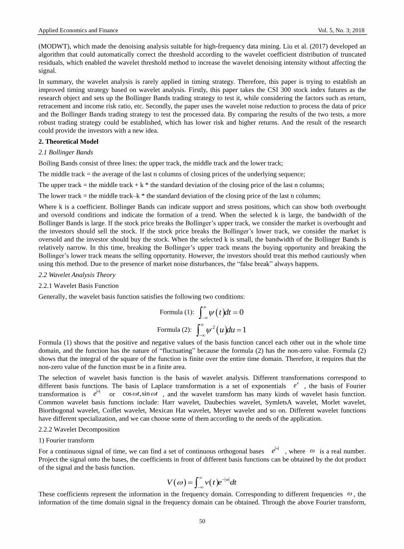
Figure 7. Normalized signal trend

3.3.1.2 Wavelet Noise Reduction

The purpose of wavelet noise reduction is to reserve the effective scale coefficient and wavelet coefficient as much as

possible and remove or lower the scale coefficients and the wavelet coefficients generated by noise.

This paper chooses sym wavelet as the wavelet basis function and chooses 4 as the vanishing moment of wavelet noise

reduction, that is sym4. When decomposing and reconstructing the denoised signal, this paper chooses 3 as the

vanishing moment(sym3). Because the number of decomposition layers will affect the denoising effect, this paper

chooses 3 as the number of the decomposition layer.

This paper performs threshold processing on the scale coefficients and the wavelet coefficients for each layer obtained

by decomposition. The following model is selected：

2log( )thr n Where n is the signal length, σ is the noise intensity, also known as signal to noise ratio.

Firstly this paper uses the MATLAB to calculate the threshold thr and obtain its value 0.0064, then reconstruct the

threshold-processed layer’s coefficients. As shown in Figure 8, take the one-minute signal line on December 23, 2012

and compare the signal before and after the noise reduction process, we can see that the processed signal is smoother.

Figure 8. The signals before and after the noise reduction

3.3.1.3 Wavelet Decomposition and Reconstruction

Wavelet decomposition and reconstruction have been mentioned in 3.3.1.2, here comes the multi-resolution

decomposition and reconstruction of the signal that has experienced the noise reduction. The structure of coefficient is

shown in Figure 9:

Applied Economics and Finance Vol. 5, No. 3; 2018

56

Signal(s)

ca1 cd1

ca2 cd2

ca3 cd3

ca3 cd3 cd2 cd1

Figure 9. Coefficient structure of three - layer signal wavelet decomposition

Figure 9 shows a process of three-layer multi-resolution decomposition on the denoised signal and the structure of

coefficients in each layers. In figure 9, the scale coefficient 3ca corresponds to the low-frequency part of the

coefficient and the wavelet coefficients 3cd , 2cd and 1cd correspond to the high frequency part of the coefficient.

After obtaining the third-level scale coefficients and the wavelet coefficients of each layer, this paper reconstruct the

coefficients of each layer and analyzed them respectively. As shown in Figure 10, there is a strong noise in the signal

which means that the usage of Bollinger Bands trading strategy to identify the buying and selling points are prone to

mistakes.

Figure 10. The scale signal of the CSI300 stock index futures and the reconstruction of the wavelet signals in each layer

3.3.2 Bollinger Bands Trading Strategy Test Based on Wavelet Analysis

After using the Bollinger Bands trading strategy to test the data that has been processed by the wavelet noise reduction,

we can get the Table 2 and the Figure 11 as follows:

Table 2. Bollinger Bands Trading Strategy Based on Noise Reduction Data

Bollinger Bands trading strategy based on wavelet analysis Final profit (RMB) 845256 Income risk ratio 373

The maximum retracement (RMB) 115440 Number of transactions 1.7163

Applied Economics and Finance Vol. 5, No. 3; 2018

57

Figure 11. Profit after noise reduction

Table 2 shows that the Bollinger Bands trading strategy based on wavelet analysis has fewer transactions and higher

profit, while the income risk ratio is close to 2. As shown in Figure 6, the overall profit shows a steady upward trend

with a small fluctuation after noise reduction.

3.4 Comparative Analysis of Different Trading Strategies

Different values of the indicators between the two trading strategy are shown in Table 3:

Table 3. the comparison between the strategies

Bollinger Bands trading

strategy Bollinger Bands trading strategy based

on wavelet analysis

Final profit (RMB) 269818 845256 Number of transactions 465 373

The maximum retracement (RMB) 133753 115440 Income risk ratio 0.4729 1.7163

As shown in Table 3, when compared with the original Bollinger Bands trading strategy, the Bollinger Bands trading

strategy based on wavelet analysis has greatly increased the final profit and the risk-return ratio, while significantly

reducing the number of transactions and the maximum retracement. This shows that the wavelet analysis is able to

reduce the judgment error of the Bollinger channel resulting from the “false break”, and it also reduces the transaction

loss and makes the model perform better. To some extent, the wavelet analysis has important enlightenment and

reference significance to other trend trading strategies.

4. Conclusion

This paper uses the CSI 300 stock index futures as the research object and selects four indicators including the final

profit, the number of transactions, the maximum retracement, and the income risk ratio as the criterions. By using the

Bollinger trading strategy and the Bollinger Bands trading strategy based on wavelet analysis to test the data of CSI 300

stock index futures, the results show that the Bollinger Bands trading strategy based on wavelet analysis is able to

effectively prevent the occurrence of the “false break”. Therefore, it can reduce the transaction errors and the number of

transactions and at the same time bring more profits with relatively smaller risks and better performance.

With the rapid development of financial innovation in China capital market, more and more varities of stock index

futures and short selling mechanisms will be introduced into the stock market, while the investors' trading ideas and

techniques will also change accordingly. Quantitative trading strategy will play a crucial role in this process. In

response to the problem of timing errors in buying and selling points caused by “false break” in the timing strategy of

Bollinger Bands, this paper proposes a method of using wavelet analysis to reduce noise. It can effectively reduce the

number of transactions caused by wrong signals, which shows great importance because the commission rate has been

greatly increased nowadays. What’s more, the method of noise reduction by wavelet analysis has important

enlightenment and reference significance to other timing strategies.

The wavelet analysis has two main applications including signal noise reduction and multi-scale analysis. In addition to

the application described in this paper, it can also be more widely used in quantitative transactions:

1) Signal noise reduction: the noise signals may contain unexpected market information from market, which can be

used to study unexpected situations in the market and help to guide rational investment. In addition, it can be used

not only in the price variable but also in other variables such as the transaction volume;

2) Multi-scale analysis: historical data can be analyzed on different time scales to analyze the performance of market

data such as prices in different market cycles, as well as to analyze past market trends.

Applied Economics and Finance Vol. 5, No. 3; 2018

58

References

Edward, W. S., & Thomas, M. (2012). A new wavelet-based denoising algorithm for high-frequency financial data

mining. European Journal of Operational Research, 217(3), 589-599. https://doi.org/10.1016/j.ejor.2011.09.049

Gençay, R., Selçuk, F., & Whitcher, B. J. (2002). Wavelet Denoising - An Introduction to Wavelets and Other Filtering

Methods in Finance and Economics – 6, 12(3), 202–234.

Grossmann, A., & Morlet, J. (1984). Decomposition of Hardy function into square integrable wavelets of constant shape.

SIAM J. Math. Anal., 15(4), 723–736. https://doi.org/10.1137/0515056

Li, Z. (2013). Quantitative investment trading strategy research. Tianjin University.

Liu, B., Huang, Q., & Zhang, W. et al (2017). Study on wavelet denoising method and its application to set background

error variance. Acta Physica Sinica, 66(2), 85-93. http://dx.doi.org/10.7498/aps.66.020505

Madhavan, A. N. (2002). VWAP strategies. Trading Spring, (1), 32-39.

Su, B. (2015). Quantitative timing based on PCA-SVM model. Tianjin University of Finance and Economics.

Wongsasutthikul, P. (2012). Hurst trading with an excursion into fractal space of returns. Cornell University.

Xie, D. (2016). Quantitative trading strategy overview and new strategy design. Zhejiang University.

Copyrights

Copyright for this article is retained by the author(s), with first publication rights granted to the journal.

This is an open-access article distributed under the terms and conditions of the Creative Commons Attribution license

which permits unrestricted use, distribution, and reproduction in any medium, provided the original work is properly

cited.