Connors Research Trading Strategy Series 

Bollinger Bands®  

Trading Strategies  

That Work By 

Connors Research, LLC 

Laurence Connors 

Cesar Alvarez 

   

2 | P a g e   

Copyright © 2013, Connors Research LLC. ALL RIGHTS RESERVED. No part of this publication may be reproduced, stored in a retrieval system, or transmitted, in any form or by any means, electronic, mechanical, photocopying, recording, or otherwise, without the prior written permission of the publisher and the author. This publication is designed to provide accurate and authoritative information in regard to the subject matter covered. It is sold with the understanding that the author and the publisher are not engaged in rendering legal, accounting, or other professional service. Authorization to photocopy items for internal or personal use, or in the internal or personal use of specific clients, is granted by Connors Research, LLC, provided that the U.S. $7.00 per page fee is paid directly to Connors Research, LLC, 1-973-494-7333. ISBN 978-0-9886931-9-7

Printed in the United States of America.

3 | P a g e   

Disclaimer

By distributing this publication, Connors Research, LLC, Laurence A. Connors and Cesar Alvarez (collectively referred to as “Company") are neither providing investment advisory services nor acting as registered investment advisors or broker-dealers; they also do not purport to tell or suggest which securities or currencies customers should buy or sell for themselves. The analysts and employees or affiliates of Company may hold positions in the stocks, currencies or industries discussed here. You understand and acknowledge that there is a very high degree of risk involved in trading securities and/or currencies. The Company, the authors, the publisher, and all affiliates of Company assume no responsibility or liability for your trading and investment results. Factual statements on the Company's website, or in its publications, are made as of the date stated and are subject to change without notice. It should not be assumed that the methods, techniques, or indicators presented in these products will be profitable or that they will not result in losses. Past results of any individual trader or trading system published by Company are not indicative of future returns by that trader or system, and are not indicative of future returns which be realized by you. In addition, the indicators, strategies, columns, articles and all other features of Company's products (collectively, the "Information") are provided for informational and educational purposes only and should not be construed as investment advice. Examples presented on Company's website are for educational purposes only. Such set-ups are not solicitations of any order to buy or sell. Accordingly, you should not rely solely on the Information in making any investment. Rather, you should use the Information only as a starting point for doing additional independent research in order to allow you to form your own opinion regarding investments. You should always check with your licensed financial advisor and tax advisor to determine the suitability of any investment. HYPOTHETICAL OR SIMULATED PERFORMANCE RESULTS HAVE CERTAIN INHERENT LIMITATIONS. UNLIKE AN ACTUAL PERFORMANCE RECORD, SIMULATED RESULTS DO NOT REPRESENT ACTUAL TRADING AND MAY NOT BE IMPACTED BY BROKERAGE AND OTHER SLIPPAGE FEES. ALSO, SINCE THE TRADES HAVE NOT ACTUALLY BEEN EXECUTED, THE RESULTS MAY HAVE UNDER- OR OVER-COMPENSATED FOR THE IMPACT, IF ANY, OF CERTAIN MARKET FACTORS, SUCH AS LACK OF LIQUIDITY. SIMULATED TRADING PROGRAMS IN GENERAL ARE ALSO SUBJECT TO THE FACT THAT THEYARE DESIGNEDWITH THE BENEFIT OF HINDSIGHT. NO REPRESENTATION IS BEING MADE THAT ANY ACCOUNT WILL OR IS LIKELY TO ACHIEVE PROFITS OR LOSSES SIMILAR TO THOSE SHOWN. Connors Research 10 Exchange Place Suite 1800 Jersey City, NJ 07302

4 | P a g e   

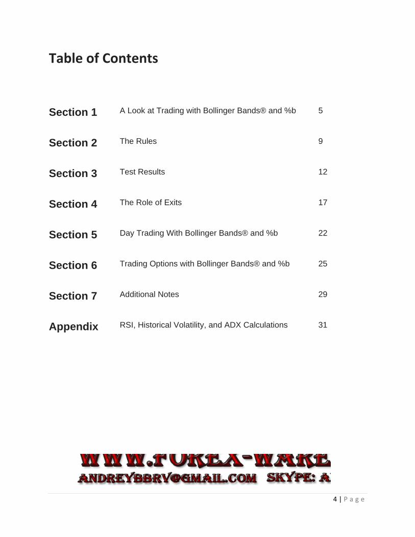
Table of Contents 

Section 1 A Look at Trading with Bollinger Bands® and %b 5

Section 2 The Rules 9

Section 3 Test Results 12

Section 4 The Role of Exits 17

Section 5 Day Trading With Bollinger Bands® and %b 22

Section 6 Trading Options with Bollinger Bands® and %b 25

Section 7 Additional Notes 29

Appendix RSI, Historical Volatility, and ADX Calculations 31

 

 

 

 

 

5 | P a g e   

Section 1

A Look at Bollinger 

Bands® and %b  

6 | P a g e   

Created by legendary money manager and researcher John Bollinger, Bollinger Bands® are one 

of the most popular indicators applied by traders throughout the world in nearly all markets. 

It’s rare today to see a chart not accompanied by Bollinger Bands® as they’ve become a must 

have visualization tool which allows traders to see how overbought or oversold a security is. 

There has been an abundance of information published on how to trade with Bollinger Bands®. 

Much of it though is discretionary in theory. The how‐to‐use Bollinger Bands® information 

usually pushes it back to the trader to interpret what the security’s price is doing relevant to its 

Bands.   

This Guidebook does not.  

What you will learn is how to exactly identify overbought and oversold key levels with Bollinger 

Bands® and applying them knowing what the historical returns have been when they reached 

specific levels.   

With the Trading with Bollinger Bands® Strategy Guidebook, you will learn how to identify the 

best historical entry and exit triggers, along with multiple levels of intraday pullbacks to 

increase the edges of the Bands. We’ll also teach you various exit points to allow for even more 

flexibility in your trading. 

We looked at every United States stock which has traded on average at least 250,000 shares a 

day priced above $5 a share from January 2001‐May 2012 (the date we started writing the 

Guidebook). This includes all stocks along with those that were bought out, delisted, etc. You 

are seeing Bollinger Bands®, and especially the %b component of Bollinger Bands® in play every 

day on all liquid stocks for over a decade. From this you will see that the %b component of 

Bollinger Bands® has had significant predictive ability to short‐term prices when it’s properly 

applied.  As a whole, you have one of the most robust quantified equity strategies for applying 

Bollinger Bands®. 

Before describing the strategy, let’s look at exactly what Bollinger Bands® are and also what we 

consider to be the genius within the Bollinger Bands®‐ the %b calculation ‐ which we will 

specifically focus on. 

7 | P a g e   

What Are Bollinger Bands®? 

Bollinger Bands® are used to measure the highness or lowness of the price relative to previous 

trades. 

For the strategies in this Guidebook, Bollinger Bands® consist of: 

  • an upper band at 1 times a 5‐period standard deviation above the moving average. 

  • a lower band at 1 times a 5‐period standard deviation below the moving average. 

The closer a security is to its lower level, the more oversold it is. The closer a security it is to its 

upper level, the more overbought it is. 

Most research and strategies revolving around Bollinger Bands® use this concept and then tend 

to add other filters to this to create a strategy. As was just mentioned, few if any provide exact 

rules with multiple years of test results. In this Guidebook we have gone further by doing this 

for you. 

In our opinion (which is backed by statistical results), the %b component of the Bollinger 

Bands® allows you to better pinpoint proper entry and exit levels when trading stocks. 

%b is an indicator derived from Bollinger Bands®, and quantifies a security's price relative to the 

upper and lower Bollinger Band.   

The default setting for %b is based on the default setting for Bollinger Bands® (5,1). The bands 

are set 1 standard deviation above and below the 5‐day simple moving average, which is also 

the middle band. The security price is the close (or the last trade for intraday readings). 

Here is the Calculation for %b 

%b = (Price ‐ Lower Band)/(Upper Band ‐ Lower Band) 

%b equals 1 when price is at the upper band 

%b equals 0 when price is at the lower band 

%b is above 1 when price is above the upper band 

%b is below 0 when price is below the lower band 

%b is above .50 when price is above the middle band (5‐day SMA) 

%b is below .50 when price is below the middle band (5‐day SMA) 

Ideally when buying a security we want the %b reading to be below 0.1 for multiple days. The 

lower the %b reading and the more days in a row below that reading, the more oversold the 

security is and the greater the historical edges have been.  This is the key to trading with 

8 | P a g e   

Bollinger Bands® and by applying a few additional filters, you are then able to build strategies 

with high average gains per trade and high success rates over the past 11+ years.   

You can plot the %b indicator at StockCharts.com (settings: 5,1). 

Let’s now go to the exact rules and parameters and then look at the historical test results.

9 | P a g e   

Section 2

The Rules 

10 | P a g e   

When you’re trading with Bollinger Bands® and especially the %b component of Bollinger 

Bands® you want to be as structured and rule‐based as possible. Let’s now go to the rules for 

trading in stocks.  

1.  The stock must be above $5 per share. 

2.  The stock’s average daily volume over the past 21 days (one trading month) must be 

at least 250,000 shares per day. This assures we’re in liquid stocks. 

3.  The stock’s 100‐day historical volatility is above 30.  (See the Appendix for a 

definition of historical volatility). 

4.  The stock’s 10 day Average Directional Index (ADX) is above 30. (See the Appendix for 

a definition of ADX). 

5.  The stock closes above its 200‐day moving average. 

6.  The %b of the stock must be under X (X=0.1, 0, ‐0.1) Y days in a row (Y = 2, 3, 4). A 

close under 0 has the stock closing under its lower band. 

7.  If the above rules are met, buy the stock tomorrow on a further intraday limit Z% 

below today’s closing price (Z= 4%, 6%, 8%, or 10%). 

8.  Exit the position when its %b closes above 1.0 (its upper band), exiting at the closing 

price. We’ll also show the test results exiting when the stock closes above a %b level of 

0.50, 0.75, on the first up close, using 2‐period RSI exits, moving average exits, and 

exiting the same day (day trade). The goal here is to empower you with as much 

knowledge as possible when exiting the trade. 

Let’s now go deeper into Rules 3‐8.  

Rules 3 and 4 assure that the stock has enough volatility in order to allow for larger moves. 

Rule 5 assures that the stock is in a longer‐term uptrend. 

Rule 6 is there to identify the pullback. A stock that closes below a %b level of 0.1 multiple days 

in a row is a good short‐term pullback. We want the %b component of the Bollinger Bands® to 

be under a low level multiple days in a row. The lower the %b level of a stock, the more the 

stock is oversold and the greater its returns have been over the next one to two weeks. 

Rule 7 helps make the %b pullback really stand‐out. Whereas most pullback methods may have 

small edges, this rule assures that the pullback is even deeper and because it’s occurring 

intraday, it’s often accompanied by a lot of fear. Money managers especially get nervous and 

11 | P a g e   

often tell their head traders to “just get me out” after they have made the decision to sell. This 

panic creates the opportunity. We want to buy the stock on an intraday basis on a further 

pullback intraday with a limit order. What we are doing is taking an already oversold stock as 

measured by the %b and then waiting for it to become even more oversold intraday. 

Rule 8 assures that we have a disciplined, quantized exit in place. Few strategies have 

quantified, structured, and disciplined exit rules. Rule 8 gives you the exact parameters to exit 

the trade backed by over a decade of historical test results. 

Let’s now look at the test results. 

12 | P a g e   

Section 3

Test Results 

13 | P a g e   

When traders ask what is a good edge (meaning the average gain per trade) on a short–term 

basis (three to ten trading days), the rule of thumb is ½% up to 2.5% per trade. This includes all 

trades. 

The average gain per trade is the number of winning trades times their average gain minus the 

losing trades times their average loss divided by the total trades. So, if is system has a total of 

100 trades and 60% make 2% on average and 40% lose 1% on average you have 120% minus 

40% divided by 100. In this example the average gain per trade is 0.80%. 

Short‐term edges on the long side often exist because of fear. This fear is a manifestation of the 

market participants and takes the form of market fear and/or individual stock fear. The greatest 

edges appear when fear is at the highest. When everyone becomes afraid, they sell their stocks 

mostly out of preservation. Think of the known phenomenon of fight or flight. When there is 

mass selling, traders and investors are in flight mode. And this is where securities become 

mispriced on a short‐term basis and the opportunities arise. 

There are a number of components to market fear. The two most prevalent are caused by large 

price sell‐offs, or shocks to the market. The other is caused by time. We’ve seen this over and 

over again in quantified testing. The longer the sell‐off, the greater the fear that sets in, and the 

greater the edges that exist. 

A third aspect is intraday fear. It’s one of the most powerful yet least written about aspects of 

trading. Take a stock (or market), sell it off multiple days and then hit it hard intraday. That 

intraday sell‐off is often pure panic. And when they panic, they sell at any price and create large 

opportunities for you. You’ll see this when we look at the Bollinger Bands® strategy and look to 

buy intraday at extreme intraday pullback levels. The historical returns (edges) are extremely 

high. 

Let’s now look at the top 20 returns per variation of The Bollinger Bands® Strategy. These are 

the returns for the 11+‐year period from January 2001‐May 2012 (the time this is being 

written). With these test results we’ll use an exit when the stock closes above its %b reading of 

1.0. In a later chapter we’ll look at the results using other exits.  

The gains and edges here have been substantial, especially for the largest intraday pullbacks; 

those that have pulled back 6% up to 10%. 

14 | P a g e   

Table 3.1. Top 20 Strategies Based on Average Gain Per Trade 

 

15 | P a g e   

Here is an explanation of each column: 

# Trades is the number of times this variation triggered from January 1, 2001‐May 31, 2012. 

Each variation has had hundreds and in some cases over 1000 signals trigger. 

Average % Profit/Loss is the average gain for all trades (including the losing trades). The top 20 

variations have shown gains on average from 4.55% per trade all the way up to 7.86% (an 

extremely high number for stocks). 

Average Days Held is the number of days on average the trade was held. In all cases it’s in the 6 

to 8 day range. 

% of Winners is the % of signals which closed out at a profit. The majority have been above 

70%, an extremely high level, especially in a world where most successful traders look to be 

correct 55%‐60% of the time. 

Exit Method is a %b close above 1.0. We’ll look at other exits as we move ahead. 

Entry Limit is the intraday pullback used to trigger an entry. This means that the buy trigger 

occurs the next day X% below the signal day. Therefore if today comes in with a signal, the 

signal is executed only if the stock pulls back further. In our testing we looked at 4%‐10% limits. 

As you can see 8% and 10% predominate the list and further reinforce the fact that the larger 

the intraday pullback, the greater the edges have been using Bollinger Bands®. 

%b Cut‐Off is the %b Level. We tested 0.1, 0.0 and ‐0.1. The test results predominantly show 

that the lower the %b level, the more oversold the stock is and the better the historical returns 

have been. 

Days Under is the number of days under the %b cut‐off level. We tested two, three, and four 

days under the %b cut‐off level. As you can see, the more days the stock is under its cut‐off 

level, the more oversold the stock is and the higher the average gains per trade have been. 

The two best performing variations have been 4 days under 0.0 or ‐0.1 with a 10% limit order. 

The ‐0.1 cut‐off level doesn’t occur as often and therefore the 0.0 level is preferred as it gives 

more trades. 

What you have here is 20 different variations of %b showing consistent behavior over more 

than a decade’s period of time. The key is to lock down the variation or variations that fit best 

for you and then apply them in a systematic structured trading manner. %b as applied with 

these rules has shown consistent healthy edges for over a decade. 

Let’s now look at the 20 highest performing variations by percentage correct using the same 

exit. 

16 | P a g e   

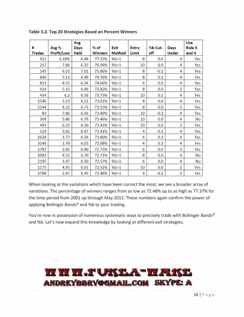
Table 3.2. Top 20 Strategies Based on Percent Winners 

 

When looking at the variations which have been correct the most, we see a broader array of 

variations. The percentage of winners ranges from as low as 72.48% up to as high as 77.37% for 

the time period from 2001 up through May 2012. These numbers again confirm the power of 

applying Bollinger Bands® and %b to your trading. 

You’re now in possession of numerous systematic ways to precisely trade with Bollinger Bands® 

and %b. Let’s now expand this knowledge by looking at different exit strategies. 

 

 

17 | P a g e   

Section 4

The Role of Exits 

18 | P a g e   

In this section, we’re going to expand your knowledge of trading with Bollinger Bands® by 

introducing various exit strategies. As you will see, these exit strategies improve the historical 

results even further and provide you with greater opportunities to trade with Bollinger Bands® 

and %b.  

We looked at seven different exit strategies.  

They are: 

1.  a %b reading of above 1.0. 

2.  a %b reading of above 0.75. 

3.  a %b reading of above 0.50. 

4.  a 2‐period RSI above 70. 

5.  a 2‐period RSI above 50. 

6.  closing price above the 5‐period simple moving average. 

7.  closing price above the 3‐period simple moving average. 

Here are the results of the best performing variations combined with the exits. 

19 | P a g e   

Table 4.1. Top 20 Strategies Based on Average Gain Per Trade 

 

A close above a %b reading of 1.0 is still the best performing variation. When you add in the 

other exits you now see all 20 variations averaging over 6% per trade. The robustness has 

increased and you now have multiple exit points you can use to exit your positions. 

20 | P a g e   

Table 4.2. Top 20 Strategies Based on Percent Winners 

 

Two main things stand out: 

1.       By looking at the additional exit strategies, the % correct goes up by a healthy amount. 

We now see strategy variations showing percent correct levels of 77.61% all the way up to 

82.76%. 

2.       The average holding period for the trades drops significantly, especially for exits such as a 

closing price above the 3‐period simple moving average. The edges are less than the other exit 

strategies but in many cases the holding period is cut in half. This further allows you to decide 

which variations and exits fit you best. 

21 | P a g e   

Summary 

As you can see, knowing how to exit a Bollinger Bands® trade is as important as knowing when 

to enter one. By looking at various precise exit points, you’re able to see more variations with 

high edges and a historically high probability of trading success. 

 

22 | P a g e   

Section 5

Day Trading with  

Bollinger Bands® 

23 | P a g e   

Even though this is not a day trading Guidebook, we wanted to show you the intraday edges 

that exist with specific variations. These variations can be automated for your trading. 

Successful day trading is mostly a game of pennies. The best firms and individual traders who 

day trade look to scalp for a small amount. Using Bollinger Bands® and %b as taught in the 

previous chapters show that intraday edges do exist. 

The larger day trading firms look for edges as little as 0.1% up to 0.5% per trade (they can trade 

for tiny commission amounts along with receiving rebates). Individual traders need larger edges 

and those edges are often difficult to find over longer‐term periods of time.  By using Bollinger 

Bands® though we can see that edges have existed for over a decade. 

Below you will see the 10 largest intraday historical edges ranging from 1.5% per trade up to 

1.87% per trade. 

Table 5.1. The Ten Largest Intraday Bollinger Band® Strategy Historical Edge 

 

The variation that intrigues us the most is the 7th one, which requires the setup day to only 

have two consecutive days with %b readings under 0.1, followed by buying the stock at a 10% 

limit and exiting on the close. 

There have been 4845 simulated trades since 2001 with over 65% of the signals being profitable 

(this is very high for any day trading strategy) and an average gain of 1.63% per trade (over 

three times higher than what the best trading firms strive for). Because these setups occur so 

often they offer traders ample opportunities throughout the year. 

24 | P a g e   

Summary 

With overnight positions the stocks need to be at extreme Bollinger Bands® and %b levels. For 

day trading this is not the case. Simply having a stock at a basic %b oversold level and then 

waiting for it to sell‐off intraday by 8%‐10% allows for numerous trades to trigger at high 

success rates with healthy intraday edges. 

25 | P a g e   

Section 6

Trading Options with 

Bollinger Bands® 

26 | P a g e   

Please note that the options section in the majority of the Connors Research Trading Strategy 

Series is the same because the strategy setups often involve large moves in brief periods of time. 

In our opinion, and confirmed from friends who are professional options traders (one with over 

three decades of experience); there is one best way to trade moves like these. 

Options trading has been a major growth industry over the past 5 years in the markets. This is 

because spreads have tightened, liquidity has increased and the ability to easily trade complex 

options has never been simpler. 

We’ll now focus on applying options trading to the short‐term market moves we have just 

learned.  Like everything else in this Guidebook, there are definitive rules as to how to execute 

an options trade when a strategy signal triggers. 

Here is what we know based upon the data: 

1.  The majority of the moves from entry to exit have been held a very short period of 

time (6‐7 trading days). 

2.  The average gains per trade have been large – well beyond the normal distribution of 

prices over that short period of time. 

3.  A high percentage of the moves have been correct. 

When we look at this type of behavior, it can lead to many strategies but one strategy stands 

out (and this has been confirmed by professional traders). The strategy is to buy front month, 

in‐the‐money long calls. 

Why front month in‐the‐money long calls?  Because they will move the closest to the stock 

itself. And the closer an option moves with the stock, the greater the gain will be on a 

percentage basis when the move is correct. 

Here are the rules. 

1.  A signal triggers. 

2.  Buy the front month in‐the‐money call. If you were to normally buy 500 shares of 

stock, buy 5 calls (every 100 shares should equal one call). 

3.  Exit the options when the signal triggers an exit on the stock. 

Let’s go further: 

1.  What does in‐the‐money exactly mean here? 

27 | P a g e   

In this case it’s defined as one to two strike prices in the money.  If the stock is at 48, buy the 40 

or 45 calls. 

2.  What does front month mean? 

Because the holding period is so short, you want to trade the options whose monthly expiration 

is the closest.  If the closest month is 7 trading days or less from the front month’s option 

expiration date (meaning the second Thursday before or closer) use the following month as the 

one to trade. 

3.  What happens if I’m in the position and it expires yet the signal for the stock is still valid? 

In this case, roll to the next month. You’re trading the stock signals so you want to have 

exposure to that signal. 

4.  What about liquidity and spreads? 

There’s some discretion here. There is no hard and fast rule as to what exactly liquidity means 

in options.  For example, compare the liquidity of your stock to SPY, which is extremely liquid 

compared to a blue chip stock. Both can be considered liquid, but the blue chips option will be 

less liquid than SPY. 

Assuming there is active volume in the options, look at the spreads.  If the option is trading 3.00 

bid ‐3.30 offer, the spread is 10%.  Can you really overcome a 10% spread?  Not likely. Now 

compare this to an option that’s trading at 3.25 bid – 3.30 offer.  This is far more acceptable 

and tradable. 

5.  What are the advantages of buying call options instead of the stock? 

Assuming the spreads and liquidity are there, the advantages are large: 

1.  Greater potential ROI on capital invested. 

2.  Less money tied up. 

3.  Less points at risk. This means if a stock signals at 50, it can lose up to 50 points. The 

options can only lose up to the premium you paid.  So, if you bought the 45 calls, the 

risk is only the premium. 

4.  There’s greater flexibility.  For example, let’s say the stock triggered a buy signal at 50 

and you paid 5.50 for the 45 calls. If the stock immediately moves higher (let’s say to 

56); you have choices here. You can exit, or you can roll into the 50 calls getting most 

28 | P a g e   

of your money out and now turning this into a nearly free trade if you believe that 

prices will continue to run. 

There are numerous examples like this and you can find these types of strategy opportunities in 

most options books. But trading anything exotic or different other than simply buying the calls 

is against the advice of the many professionals we posed this question to. 

In conclusion, options provide traders with a good alternative to buying the outright stock. The 

structured methodology for our strategies is: front‐month, in‐the‐money, with equivalent sizing 

(1 option per 100 shares), and exiting when the signal exits. 

The above options strategy, in many experts’ opinion, is the best and most efficient strategy 

based upon the historical data from these signals. 

29 | P a g e   

Section 7

Additional Thoughts 

30 | P a g e   

1.  As you have seen throughout this Guidebook, Bollinger Bands® and especially the %b 

component of the Bollinger Bands® have had large quantified edges when you apply them in a 

systematic manner. 

2.  There is preciseness here using Bollinger Bands® in this way. Use this preciseness to your 

advantage. 

3.  There are literally hundreds of potential variations for you to use. From the depth of the %b 

level, to the number of days below that level, to the size of the limit, and to the type of exit that 

can be applied. Look at the entire scope and then identify the variation or variations that fit 

best for your trading style. 

4.  What about stops (and we include the answer to this in all our Strategy Guidebooks)? 

We have published research on stops in other publications including in our book Short Term 

Trading Strategies That Work. 

What we have found is that stops tend to lessen performance, and in many cases they 

completely remove edges. Yes, it feels good when a stock keeps moving lower and lower and a 

stop got you out. On the other side, the research which is backed by up to two decades of test 

results on many short‐term trading strategies suggests that stops get hit often and accumulate 

many, many losses. Few trading strategies can overcome these aggregated losses.  

For many traders stops are a must. Psychologically it allows them to take trades, especially 

difficult trades. Whether you use them or not is a personal choice. On the whole though, the 

edges you see in this strategy and many other short‐term strategies are lower when stops are 

applied to them. Again this is a personal choice only you can make for yourself. We know 

successful traders in both camps. 

5.  Slippage and commission were not used in the testing. Factor them into your trading (the 

entries are at limit prices so slippage is not an issue) and make sure you are trading at the 

lowest possible costs. Most firms are now allowing traders to trade for under 1 cent a share, so 

shop your business, especially if you are an active trader. The online brokerage firms want your 

business. 

6.  As you have seen here with the Bollinger Bands® Strategy, there are large edges in stocks 

which sell‐off and then sell‐off further intraday. These trades are often accompanied by fear 

and uncertainty and this is when large edges appear. Seek out these trades because as you 

have seen, they’ve been lucrative for many years. 

We hope you enjoyed this addition to the Connors Research Trading Strategy Series. If you have 

any questions about this strategy please feel free to email us at info@connorsresearch.com

31 | P a g e   

Appendix

RSI, Historical Volatility, 

and ADX Calculations 

32 | P a g e   

2‐Period RSI 

The 2‐day RSI refers to the Relative Strength Index when set to read only the past two days of 

price action. 

The Relative Strength Index (RSI) is a popular momentum oscillator developed by J. Welles 

Wilder in the 1970s. The RSI compares the magnitude of a market’s recent gains to the 

magnitude of a market’s recent losses. 

A simple formula calculates this price action into a number between 1 and 100. Markets with 

RSIs closer to 1 are considered oversold. Markets with RSIs closer to 100 are considered 

overbought. 

RSI = (100 – (100/(1+RS))) 

RS = Average of x days up closes / Average of x days down closes 

The RSI is generally set for 14‐periods. However, for short‐term ETF trading, we have found that 

a shorter time period is much more effective. See “2‐day RSI”, “RSI(4)”. 

There is a good example and explanation of the RSI found using this link: 

http://stockcharts.com/school/doku.php?id=chart_school:technical_indicators:relative_strengt

h_index_rsi 

33 | P a g e   

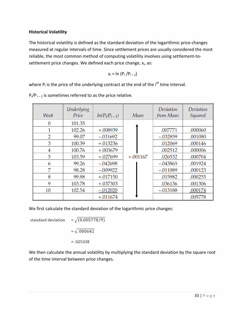
Historical Volatility 

The historical volatility is defined as the standard deviation of the logarithmic price changes 

measured at regular intervals of time. Since settlement prices are usually considered the most 

reliable, the most common method of computing volatility involves using settlement‐to‐

settlement price changes. We defined each price change, xi, as: 

xi = ln (Pi /Pi – 1) 

where Pi is the price of the underlying contract at the end of the ith time interval. 

Pi/P i – 1 is sometimes referred to as the price relative. 

 

We first calculate the standard deviation of the logarithmic price changes: 

 

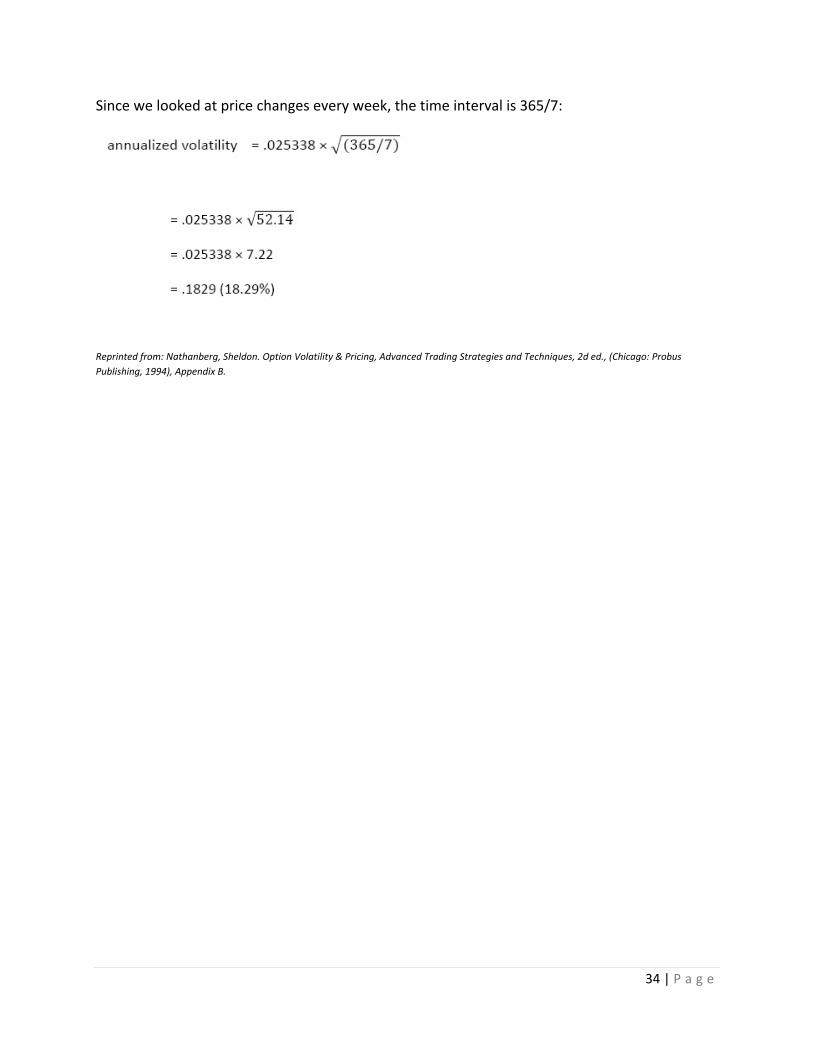
We then calculate the annual volatility by multiplying the standard deviation by the square root 

of the time interval between price changes. 

 

 

34 | P a g e   

Since we looked at price changes every week, the time interval is 365/7: 

 

 

 

 

Reprinted from: Nathanberg, Sheldon. Option Volatility & Pricing, Advanced Trading Strategies and Techniques, 2d ed., (Chicago: Probus 

Publishing, 1994), Appendix B. 

35 | P a g e   

Average Directional Index ‐ ADX 

ADX is an indicator used as a value for the strength of trend. ADX is non‐directional so it will 

quantify a trend's strength regardless of whether it is up or down.  You can find more 

information on the ADX at http://trd.mk/1C.  Also, you can click here to see how to calculate 

ADX http://trd.mk/1D or here http://trd.mk/1E.   

36 | P a g e   

More from the Connors Research Trading Strategy Series 

 

ETF Gap Trading Strategies That Work 

This Professional Approach to ETF Trading Brings You Results Quickly 

Quantitative Research Identifies Gap Strategies with Short‐Term Trades for Impressive Gains 

ETF Gap Trading Strategies That Work 

Gap Trading has proven to be a one of the longest‐standing, most successful trading strategies 

for professional traders. Over the past two decades many professional Money Managers at 

large funds, successful Commodity Advisors, and professional Equity Traders have stated they 

rely upon gaps as one of the reasons for their success. 

When traded correctly, ETF Gap Trading can be one of the most consistent strategies available 

for your trading. 

Now for the first time, we are making available to the public ETF Gap Trading: A Definitive 

Guide. 

Consistent Trading Results 

What you will learn with this strategy are dozens of gap variations which have been correct 

from 72.4% up to over 78% from 2006 to 2011.  

If you would like more information on the ETF Gap Trading Strategies That Work click here. If 

you would like to order and download it now so you can have immediate access to it please 

click here or call toll free 888‐484‐8220 ext. 1 (outside the US please dial 973‐494‐7311). 

   

37 | P a g e   

More from the Connors Research Trading Strategy Series 

 

Trading Stock Gap Trading Strategies That Work 

Gap Trading Is A “Core Strategy” For Most Successful Traders 

Do You Trade Stock Gaps? 

For three decades, gap trading has been one of the most popular and successful strategies for 

traders who have identified when and how to trade stock gaps. The problem is that there are 

literally thousands of gaps every year. So how does the average trader know which ones to 

trade, where to enter them and where to properly exit the positions? 

Now for the first time, you have the opportunity to learn what many professionals already 

know about gap trading: when it’s done correctly, it can be extremely lucrative. 

 “If I could only trade one strategy, it would be early morning gaps.” ‐‐ Kevin Haggerty, Former 

Head of Trading Fidelity Capital Markets  

Strong Results From How to Trade High‐Probability Stock Gaps ‐ 2nd Edition 

What you will learn with this strategy are dozens of short‐term set‐ups which have been correct 

greater than 68% of the time (a very high win percentage). And the average gain per trade (this 

includes all winning and losing trades) has averaged up to 6.16% per trade since 2001! 

If you rely on data, not opinion to make your trading decisions, and you want the ability to 

choose the best variations to trade your strategies, then this guide is for you. 

 If you would like more information on the Trading Stock Gap Trading Strategies That Work click 

here. If you would like to order and download it now so you can have immediate access to it 

please click here or call toll free 888‐484‐8220 ext. 1 (outside the US please dial 973‐494‐7311). 

 

38 | P a g e   

Educate Yourself on How to Succeed with High Probability Trading Systems ... 

The TradingMarkets Swing Trading College 

Do You Swing Trade? 

There are literally hundreds of books available on how to swing trade. Are you tired of looking 

at books and courses that tell you to “buy a pullback and sell it when it goes up”? 

You are going to need better, more precise information if you want to be successful with your 

swing trading. 

Now you can get the definitive answers to your questions. Answers that give you a high 

probability of success ‐‐ all quantified & backed by analysis of years of back‐tested, simulated  

historical results. 

You'll get these answers ‐‐ and the training you need ‐‐ at Swing Trading College ‐‐ the most 

popular education program offered by TradingMarkets for over 9 years running.  Swing Trading 

College is the comprehensive trading education program available to individual traders: we've 

had students come back to the classes two ‐‐ and even three times ‐‐ it's that good..  

The TradingMarkets Swing Trading College 

The TradingMarkets Swing Trading College is a complete training program that will teach you 

specific research, strategies, techniques, and tools necessary to swing trade quantitatively. The 

course agenda includes: 

1. How to Use Historical, Model‐Driven Results to Buy Pullbacks 

2. Swing Trading ETFs & Leveraged ETFs 

3. How and when to use Short Selling techniques 

4. Volatility Trading 

5. Quantified Options Income Programs 

6. Building Your "Personal Trading Business" 

o Setting Goals 

o Developing a Business Plan 

o Trading Psychology 

o Building a High‐Probability Swing Trading Portfolios 

 

You will also receive instruction in multiple quantified trading strategies, including: 

        S&P Selective Strategy 

39 | P a g e   

ETF Deep Pullbacks Strategy 

Short Selling Portfolio Strategy 

Daily VXX Strategy 

VXX Trend Following Strategy 

and more. 

If you would like more information on the TradingMarkets Swing Trading College click here. If 

you would like to order and download it now so you can have immediate access to it please 

click here or call toll free 888‐484‐8220 ext. 1 (outside the US please dial 973‐494‐7311).