Bloch waves and Bandgaps - San Jose State University

Document info Ch 6,

Bloch waves and Bandgaps

Chapter 6Physics 208, Electro-optics

Peter Beyersdorf

1

Ch 6,

Bloch Waves

There are various classes of boundary conditions for which solutions to the wave equation are not plane waves

Planar conductor results in standing waves

Waveguide and cavities results in modal structure

Periodic materials result in Bloch waves

2

E(z) = 2E0 sin (kzz) cos (ωt)

E(x, y, z) = Enm(x, y)e−ikz

!E(!r) =∫ 2π/Λ

0E( !K,!r)e−i "K·"rd !K

Ch 6,

Class Outline

Types of periodic media

dispersion relation in layered materials

Bragg reflection

Coupled mode theory

Surface waves

3

Ch 6,

Periodic Media

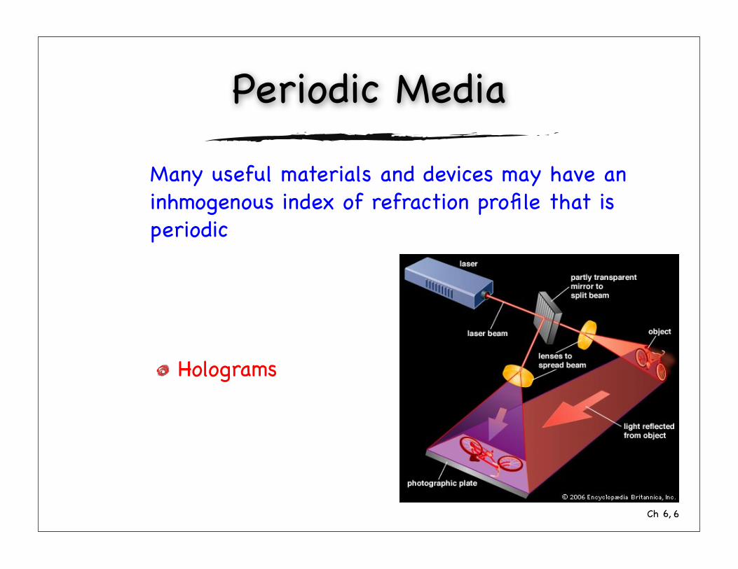
Many useful materials and devices may have an inhmogenous index of refraction profile that is periodic

Dielectric stack optical coatings

Diffraction gratings

Holograms

Acousto-optic devices

Photonic bandgap crystals

4

Ch 6,

Periodic Media




Holograms



5

Ch 6,

Periodic Media




Holograms



6

Ch 6,

Periodic Media




Holograms



7

Ch 6,

Periodic Media




Holograms



8

!E(!r) =∫ 2π/Λ

0E( !K,!r)e−i "K·"rd !K

Ch 6,

Bloch’s Theorem

Wave solutions in a periodic medium (Bloch waves) are different than in a homogenous medium (plane waves)

A correction factor E(K,r) accounts for the difference between plane wave solutions and Bloch wave solutions

Wave amplitude has a periodicity defined by the underlying medium, Ek(K,r)=Ek(K,r+Λ)

E(K,r) are normal modes of propagation

Λ

9

Ch 6,

Waves in Layered Media

For a wave normally incident on an isotropic layered material, we’ll find the “dispersion relationship” (ω vs K curve) for Bloch waves. This will tell us about the behavior of waves in the material.

We’ll see the periodic structure reflects certain wavelengths. This is referred to as Bragg reflection.

Λ

10

Ch 6,

Wave Equation in Layered Media

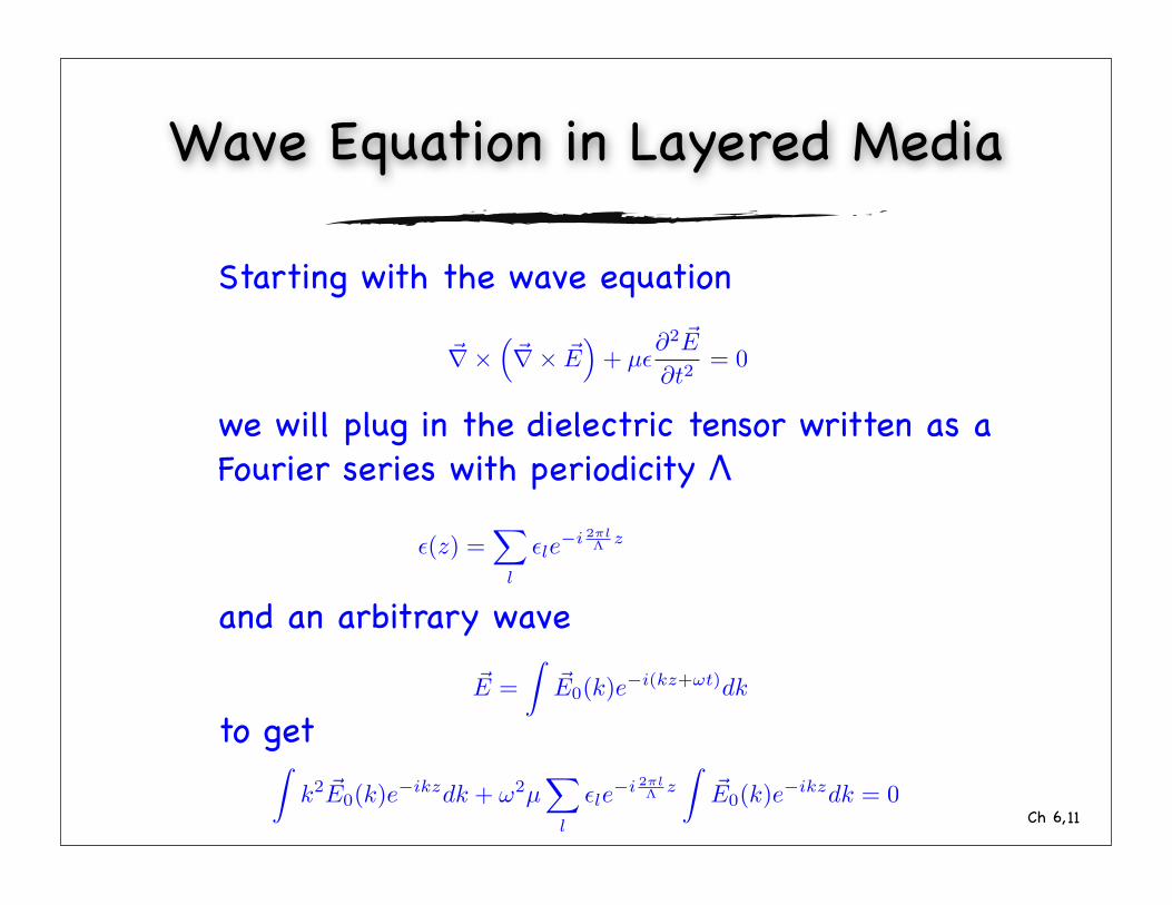
Starting with the wave equation

we will plug in the dielectric tensor written as a Fourier series with periodicity Λ

and an arbitrary wave

to get

ε(z) =∑

l

εle−i 2πl

Λ z

!E =∫

!E0(k)e−i(kz+ωt)dk

11

!∇×(

!∇× !E)

+ µε∂2 !E

∂t2= 0

∫k2 !E0(k)e−ikzdk + ω2µ

∑

l

εle−i 2πl

Λ z

∫!E0(k)e−ikzdk = 0

Ch 6,

k′ = k +2πl

Λ

for all k

and defining

with

gives

or

so

∫k2 !E0(k)e−ikzdk + ω2µ

∑

l

εle−i 2πl

Λ z

∫!E0(k)e−ikzdk = 0

∫ (k2 !E0(k)− ω2µ

∑

l

εl!E0(k −

2πl

Λ)

)e−ikzdk = 0

k2 !E0(k)− ω2µ∑

l

εl!E0(k −

2πl

Λ) = 0

12

∫k2 !E0(k)e−ikzdk − ω2µ

∫ ∑

l

εl!E0(k′ −

2πl

Λ)e−ik′zdk′ = 0


Ch 6,


for all k

Is an infinite set of equations. Consider equations for: kΛ/2π=0, 0.1, 0.2, 0.3, 0.4, 0.5, 0.6, 0.7, 0.8, 0.9, 1.0, 1.1, 1.2, 1.3 …

k2 !E0(k)− ω2µ∑

l

εl!E0(k −

2πl

Λ) = 0

coupled

Let K be the value value of k±2πl/Λ closest to ω2με0 in a series of coupled equations, where ε0 is the zeroth order Fourier coefficient of ε(z).The whole series of equations for -∞<k<∞ can be treated instead as a series of coupled equations for 0<K<2π/Λ. The solution to each set of equations for a value of K only contains terms at k=K±2πl/Λ, thus

K=0K=0.2π/Λ

K=0.4π/Λ

→ 13!E(z) =

∫!E0(k)ei(kz+ωt)dk !E(K, z) =

∑

l

!E0(K − l2π

Λ)ei(K−l 2π

Λ )z−iωt

Ch 6,

Bloch Waves in Layered Media

The Bloch waves are normal modes of propagation so

and each mode is composed of plane wave components of amplitude E(K±2πl/Λ). To find these amplitudes we consider the dispersion relation

Since this represents an infinite set of coupled equations, we will examine this expression and isolate the equations that couple most strongly to E0(K), ignore the rest and solve for E0(k)

k2 !E0(k)− ω2µ∑

l

εl!E0(k −

2πl

Λ) = 0

!E(z) =∫ 2π/Λ

0E(K, z)e−iKzdK

14

Ch 6,

Field Components in Layered Media

or

k2 !E0(k)− ω2µ∑

l

εl!E0(k −

2πl

Λ) = 0

k2 !E0(k)− ω2µεø !E0(k)− ω2µε1 !E0(k −2π

Λ)− ω2µε−1

!E0(k +2π

Λ)− . . . = 0

Allowing us to express the E0(K-2πl/Λ) amplitudes as

!E0(K) =1

K2 − ω2µεø

(ω2µε1 !E0(K − 2π

Λ) + ω2µε−1

!E0(K +2π

Λ)− . . .

)

!E0(K − 2π

Λ) =

1(K − 2π

Λ

)2 − ω2µεø

(ω2µε1 !E0(K − 2

2π

Λ) + ω2µε−1

!E0(K)− . . .

)

!E0(K +2π

Λ) =

1(K + 2π

Λ

)2 − ω2µεø

(ω2µε1 !E0(K) + ω2µε−1

!E0(K + 22π

Λ)− . . .

)

…

15

Ch 6,

Resonant Coupling of Waves

Momentum of forwards wave with wavenumber k is ℏk, for backwards wave it is -ℏk. Grating can be thought of as superposition of forwards and backwards going waves, with momenta ±ℏkg, where kg=2π/Λ. For light to couple between

forwards and backwards waves, momentum must be conserved ℏk+mℏkg=-ℏk

This is like a collision of a forward photon with m phonons producing a backwards photon

kg

k

-k

16

Ch 6,

Field Components in Layered Media

!E0(K) =1

K2 − ω2µεø

(ω2µε1 !E0(K − 2π

Λ) + ω2µε−1

!E0(K +2π

Λ)− . . .

)

!E0(K − 2π

Λ) =

1(K − 2π

Λ

)2 − ω2µεø

(ω2µε1 !E0(K − 2

2π

Λ) + ω2µε−1

!E0(K)− . . .

)

!E0(K +2π

Λ) =

1(K + 2π

Λ

)2 − ω2µεø

(ω2µε1 !E0(K) + ω2µε−1

!E0(K + 22π

Λ)− . . .

)

(K − l

2πΛ

)2! ω2µεø

K2 − ω2µεø = 0

In the case where ## # # # # # i.e. the forward wave momentum cannot be converted to the backward wave momentum by the addition of a kick from the grating in the layered material, only the l=0 term is significant and the dispersion relationfor any value of K is uncoupled to that for other values of K, and gives## # # # # meaning the phase velocity is that due to the average index of refraction for the medium

K2 !E0(K)− ω2µ∑

l

εl!E0(K − 2πl

Λ) = 0

17

Ch 6,

Coupling of Field Components

In the case where# # # # # # for some non-zero value of l=m this l=m term is also significant and for the dispersion relation

we need only consider two values of K, i.e. K and K-2πm/Λ.

l=0

l=-1

l=+1

!E0(K +2πl

Λ) =

1(K + 2πl

Λ

)2 − ω2µεø

(ω2µε1 !E0(K +

2π(l − 1)Λ

) + ω2µε−1!E0(K + 2

2πl

Λ)− . . .

)

!E0(K) =1

K2 − ω2µεø

(ω2µε1 !E0(K − 2π

Λ) + ω2µε−1

!E0(K +2π

Λ)− . . .

)

!E0(K − 2π

Λ) =

1(K − 2π

Λ

)2 − ω2µεø

(ω2µε1 !E0(K − 2

2π

Λ) + ω2µε−1

!E0(K)− . . .

)

!E0(K +2π

Λ) =

1(K + 2π

Λ

)2 − ω2µεø

(ω2µε1 !E0(K) + ω2µε−1

!E0(K + 22π

Λ)− . . .

)

K2 !E0(K)− ω2µ∑

l

εl!E0(K − 2πl

Λ) = 0

(K − l

2πΛ

)2≈ ω2µεø

18

Ch 6,

Dispersion Relation in Layered Media

A nontrivial solution to these coupled equations only exists if

k2 !E0(k)− ω2µ∑

l

εl!E0(k −

2πl

Λ) = 0The dispersion relation

Considering only terms with E(K) and E(K-2πm/Λ) gives

and for ε-m=εm* in a lossless medium, since

(K2 − ω2µεø

)#E0(K)− ω2µεm

#E0(K − 2πm

Λ) = 0

[(K − 2πm

Λ

)2

− ω2µεø

]#E0

(K − 2πm

Λ

)− ω2µε−m

#E0(K) = 0

∣∣∣∣K2 − ω2µεø −ω2µεm

−ω2µε−m

(K − 2πm

Λ

)2 − ω2µεø

∣∣∣∣ = 0

(K2 − ω2µεø

)((

K − 2πm

Λ

)2

− ω2µεø

)−

(ω2µ|εm|

)2 = 0 19

εm =1Λ

∫ Λ

0ε(z)e−i2πmz/Λdz

Ch 6,

Dispersion Relation in Layered Media

which can be solved for K, the Bloch wave vector for a wave of frequency ω

graph of dispersion relationship (figure 6.2)

(K2 − ω2µεø

)((

K − 2πm

Λ

)2

− ω2µεø

)−

(ω2µ|εm|

)2 = 0

20

K =mπ

Λ±

√√√√(mπ

Λ

)2+ εøµω2 ±

√

(|εm|µω2)2 +(

2πm

Λ

)2

εøµω2

Ch 6,

Bandgaps in Layered Media

When the Bragg condition is met (K-2πm/Λ=ω2ε0 μ)real solutions exist for# # # # # # # and

Solutions for

are complex, this region is called the forbidden band. At the center of the forbidden band where## # # # # # and## # # # # , i.e.

the dispersion relation gives

ω2 <K2

µ (εø + |εm|) ω2 >K2

µ (εø − |εm|)

K2

µ (εø + |εm|) < ω2 <K2

µ (εø − |εm|)

K2 − ω2µεø = 0(K − m

2πΛ

)2≈ ω2µεø ω2 =

(mπ)2

Λ2µεø

K =mπΛ

(1 ± i

|ε1|2εø

)

21

K =mπ

Λ±

√√√√(mπ

Λ

)2+ εøµω2 ±

√

(|εm|µω2)2 +(

2πm

Λ

)2

εøµω2

Ch 6,

Bandgap Properties

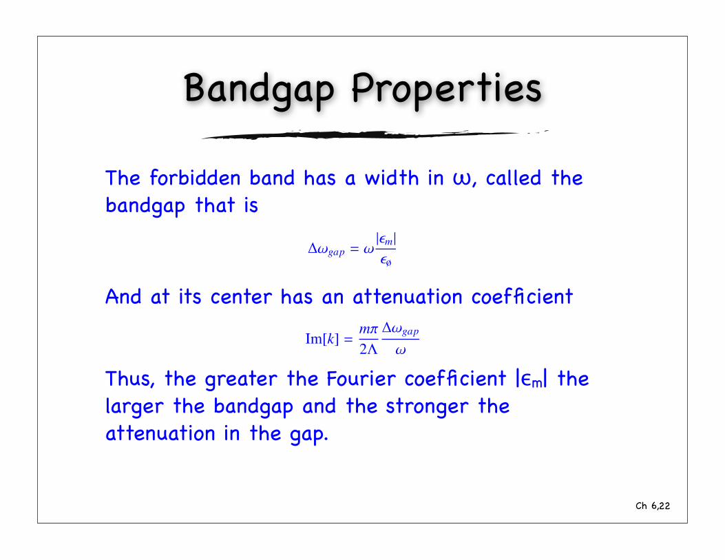
The forbidden band has a width in ω, called the bandgap that is

And at its center has an attenuation coefficient

Thus, the greater the Fourier coefficient |εm| the larger the bandgap and the stronger the attenuation in the gap.

∆ωgap = ω|εm|εø

22

Im[k] =mπ2Λ∆ωgap

ω

Ch 6,

Bloch Waveform

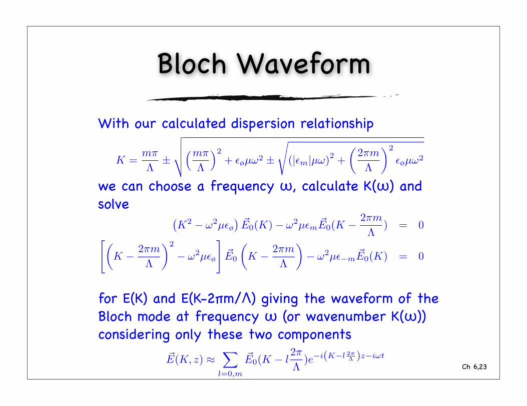
With our calculated dispersion relationship

we can choose a frequency ω, calculate K(ω) and solve

for E(K) and E(K-2πm/Λ) giving the waveform of the Bloch mode at frequency ω (or wavenumber K(ω)) considering only these two components

(K2 − ω2µεø

)#E0(K)− ω2µεm

#E0(K − 2πm

Λ) = 0

[(K − 2πm

Λ

)2

− ω2µεø

]#E0

(K − 2πm

Λ

)− ω2µε−m

#E0(K) = 0

K =mπ

Λ±

√√√√(mπ

Λ

)2+ εøµω2 ±

√

(|εm|µω)2 +(

2πm

Λ

)2

εøµω2

!E(K, z) ≈∑

l=0,m

!E0(K − l2π

Λ)e−i(K−l 2π

Λ )z−iωt

23

Ch 6,

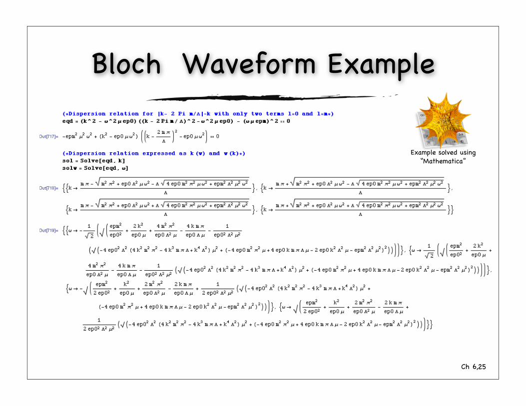
Bloch Waveform Example

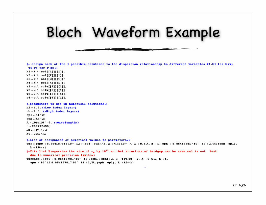
Consider a periodic structure consisting of alternating layers of high index and low index material(nh=1.8, nl=1.5).

Find the waveform in the material for a wave of wavelength λ=2Λ

nh nl

Λ=λ/2

24

Ch 6,


Example solved using “Mathematica”

25

Ch 6,


26

Ch 6,


0.9999 0.99995 1 1.00005 1.0001kêk0

0.60352

0.60354

0.60356

0.60358

0.6036

0.60362

DispersionRelation

Dispersion relation without exaggeration 27

Ch 6,


28

Ch 6,


0 1¥10-6 2¥10- 6 3¥10-6 4¥10- 6 5¥10-6

z HmL

- 20

- 10

0

10

20

Bloch wave 1

0 1¥10-6 2¥10- 6 3¥10-6 4¥10- 6 5¥10-6

z HmL

- 0.75

- 0.5

- 0.25

0

0.25

0.5

0.75

Bloch wave 2

29

Ch 6,

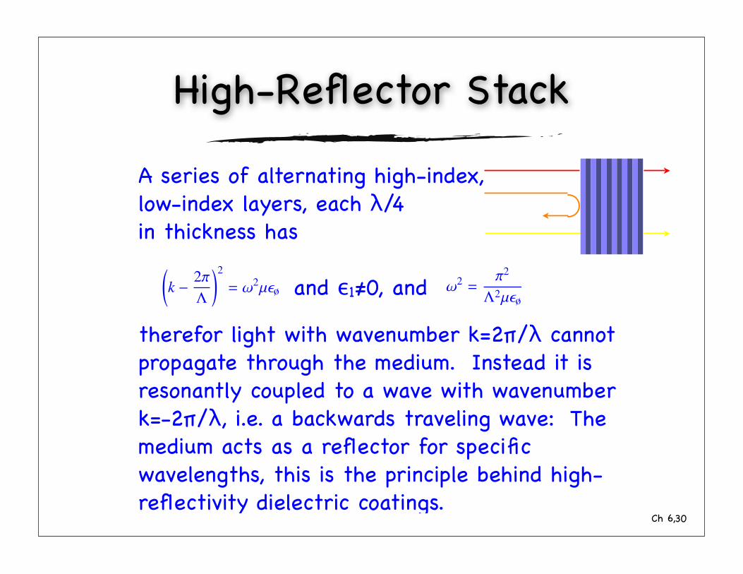
High-Reflector Stack

A series of alternating high-index, low-index layers, each λ/4 in thickness has

# # # # # # # and ε1≠0, and

therefor light with wavenumber k=2π/λ cannot propagate through the medium. Instead it is resonantly coupled to a wave with wavenumber k=-2π/λ, i.e. a backwards traveling wave: The medium acts as a reflector for specific wavelengths, this is the principle behind high-reflectivity dielectric coatings.

(k − 2πΛ

)2= ω2µεø ω2 =

π2

Λ2µεø

30

Ch 6,

Alternative Methods

In our previous method we solved the 1D wave equation for all frequencies of plane waves to get the dispersion relation.

Alternatively we can consider wave propagation in the material, impose boundary conditions at the interfaces and require self-consistent solutions to get the dispersion relation - We will apply this method for a solution in 2D to the dielectric stack problem

31

6.

∮B · dA = 0

∮E · ds = − d

dt

∫B · dA

∮εE · dA =

∑q

∮B

µ· ds =

∫J · dA +

d

dt

∫εE · dA

When an EM wave propagates across an interface, Maxwell’s equations must be satisfied at the interface as well as in the bulk materials. The constraints necessary for this to occur are called the “boundary conditions”

32

ε1, µ1 ε2, µ2

Boundary Conditions

zy

6.

∮B · dA = 0

∮E · ds = − d

dt

∫B · dA

∮εE · dA =

∑q

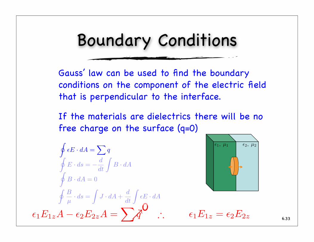
Boundary Conditions

Gauss’ law can be used to find the boundary conditions on the component of the electric field that is perpendicular to the interface.

If the materials are dielectrics there will be no free charge on the surface (q=0)

33∴→0

∮B

µ· ds =

∫J · dA +

d

dt

∫εE · dA

ε1, µ1 ε2, µ2

ε1E1z = ε2E2zε1E1zA− ε2E2zA =∑

q

6.

∮B · dA = 0

∮E · ds = − d

dt

∫B · dA

∮εE · dA =

∑q

Boundary Conditions

34

∮B

µ· ds =

∫J · dA +

d

dt

∫εE · dA

∴→0

ε1, µ1 ε2, µ2

Faraday’s law can be applied at the interface. If the loop around which the electric field is computed is made to have an infintesimal area the right side will go to zero giving a relationship between the parallel components of the electric field

E1x,y = E2x,yE2x,yL− E1x,yL = − d

dt

∫B · dA

6.

∮B

µ· ds =

∫J · dA +

d

dt

∫εE · dA

∮B · dA = 0

∮E · ds = − d

dt

∫B · dA

∮εE · dA =

∑q

Boundary Conditions

Gauss’ law for magnetism gives a relationship between the perpendicular components of the magnetic field at the interface

35∴

ε1, µ1 ε2, µ2

B1zA−B2zA = 0 B1z = B2z

6.

∮B · dA = 0

∮E · ds = − d

dt

∫B · dA

∮εE · dA =

∑q

Boundary Conditions

Ampere’s law applied to a loop at the interface that has an infintesimal area gives a relationship between the parallel components of the magnetic field. (Note that in most common materials μ=μo)

36

∮B

µ· ds =

∫J · dA +

d

dt

∫εE · dA

∴→0

→0

ε1, µ1 ε2, µ2

B1x,y

µ1L− B2x,y

µ2L =

∫J · dA +

d

dt

∫εE · dA

B1x,y

µ1=

B2x,y

µ2

6.

Reflection at a Boundary

37

Plane of the interface (here the yz plane) (perpendicular to page)

ni

nt

θi θr

θt

Ei Er

Et

Interface

x

y

z

“s” polarization (senkrecht, aka TE or vertical) has an E field that is

perpendicular to the plane of incidence

“p” polarization (parallel aka TM or horizontal) has an E field that is parallel to the plane of incidence

The reflection and transmission coefficients at an interface can be found using the boundary conditions, but they depend on the polarization of the incident light

E1x,y = E2x,y

B1z = B2z

H1x,y = H2x,y

D1z = D2z

Ch 6,

Unit Cell ConstructLabel the forwards and backwards going waves in the nth “unit cell”

an forward going wave at right side of nth unit cell inside material 1 of form

bn backward going wave at right side of nth unit cell inside material 1

cn forward going wave at right side of nth unit cell inside material 2

dn backward going wave at right side of nth unit cell inside material 2

a thickness of layer for material 1

b thickness of layer for material 2

Λ total thickness of unit celln number of unit cells to the right of some arbitrary origin

forward waves phase factor are expressed as e-ikz+iωt Λ

an

bn

cn

dn

n2 n1

Λ=a+b

ab

zy

38

Ch 6,

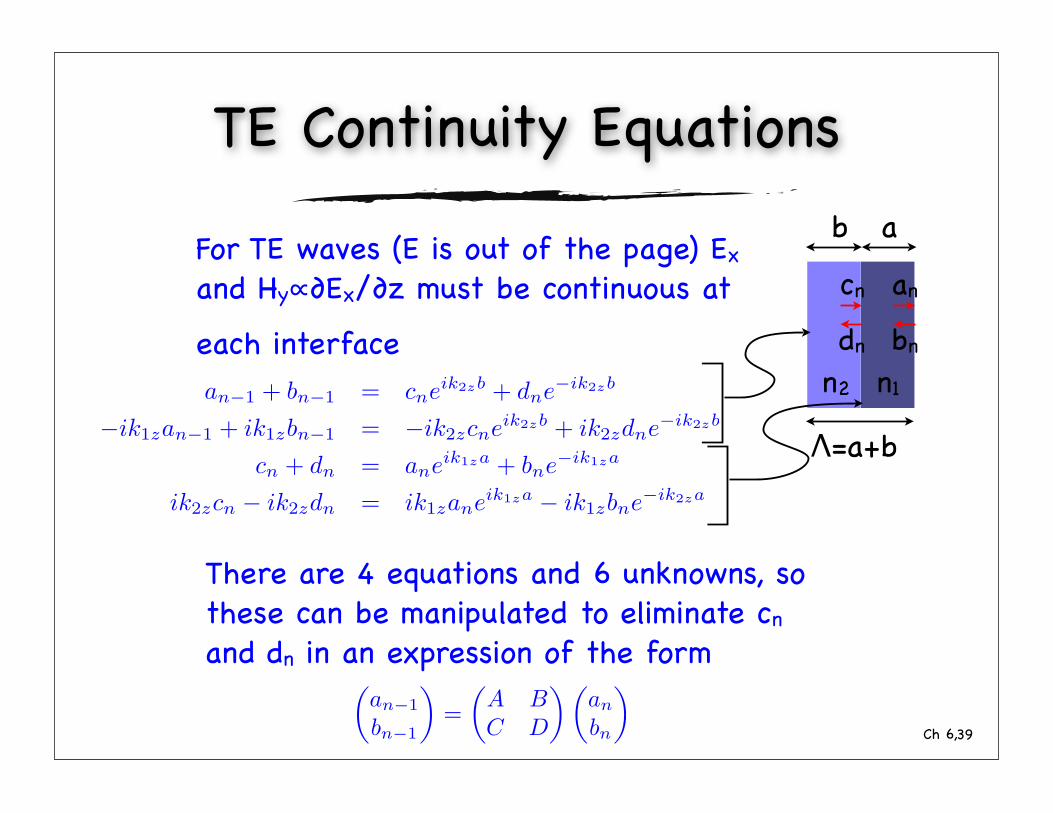
TE Continuity Equations

For TE waves (E is out of the page) Ex and Hy∝∂Ex/∂z must be continuous at

each interface

an

bn

cn

dn

n2 n1

Λ=a+b

ab

an−1 + bn−1 = cneik2zb + dne−ik2zb

−ik1zan−1 + ik1zbn−1 = −ik2zcneik2zb + ik2zdne−ik2zb

cn + dn = aneik1za + bne−ik1za

ik2zcn − ik2zdn = ik1zaneik1za − ik1zbne−ik2za

There are 4 equations and 6 unknowns, so these can be manipulated to eliminate cn and dn in an expression of the form

(an−1

bn−1

)=

(A BC D

) (an

bn

)

39

Ch 6,

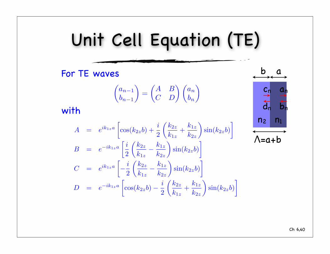
Unit Cell Equation (TE)For TE waves

with

an

bn

cn

dn

n2 n1

Λ=a+b

ab(

an−1

bn−1

)=

(A BC D

) (an

bn

)

A = eik1za

[cos(k2zb) +

i

2

(k2z

k1z+

k1z

k2z

)sin(k2zb)

]

B = e−ik1za

[i

2

(k2z

k1z− k1z

k2z

)sin(k2zb)

]

C = eik1za

[− i

2

(k2z

k1z− k1z

k2z

)sin(k2zb)

]

D = e−ik1za

[cos(k2zb)−

i

2

(k2z

k1z+

k1z

k2z

)sin(k2zb)

]

40

Ch 6,

Unit Cell Equation (TM)For TM waves

with

an

bn

cn

dn

n2 n1

Λ=a+b

ab(

an−1

bn−1

)=

(A BC D

) (an

bn

)

A = eik1za

[cos(k2zb) +

i

2

(n2

1k2z

n22k1z

+n2

2k1z

n21k2z

)sin(k2zb)

]

B = e−ik1za

[i

2

(n2

2k1z

n21k2z

− n21k2z

n22k1z

)sin(k2zb)

]

C = eik1za

[− i

2

(n2

2k1z

n21k2z

− n21k2z

n22k1z

)sin(k2zb)

]

D = e−ik1za

[cos(k2zb)−

i

2

(n2

1k2z

n22k1z

+n2

2k1z

n21k2z

)sin(k2zb)

]

41

Ch 6,

Multiple Cell PropagationFrom conservation of energy |an|2+ |bn|2= |an-1|2+ |bn-1|2 which means the ABCD matrix is “unimodular”.

For 2x2 matrices

For unimodular matrices the determinant is one,## # # # # # , so

an

bn

cn

dn

n2 n1

Λ=a+b

ab

(A BC D

)−1

=1

AD −BC

(D −B−C A

)

AD −BC = 1(

an

bn

)=

(D −B−C A

)n (a0

b0

)

42

Ch 6,

The propagating waves in the medium are bloch waves with an amplitude that is periodic in Λ and a phase given by Kz, so a bloch wave should obey

requiring

or

with the form# # # # # # # # # # where

giving

Bloch Wave Solutions

(A BC D

) (an

bn

)= eiKΛ

(an

bn

)

eiKΛ =A + D

2± i

√

1−(

A + D

2

)2

eiKΛ =A + D

2±

√(A + D

2

)2

− 1

K =1Λ

cos−1

(A + D

2

)cos ψ =

A + D

2

43

eiKΛ = cos ψ ± i sinψ = e±iψ

Ch 6,

Brewster’s angle

Contour plot Sign[Im[K(θ,ω]](stop bands are in black)

Material Bandgaps

44

Ch 6,

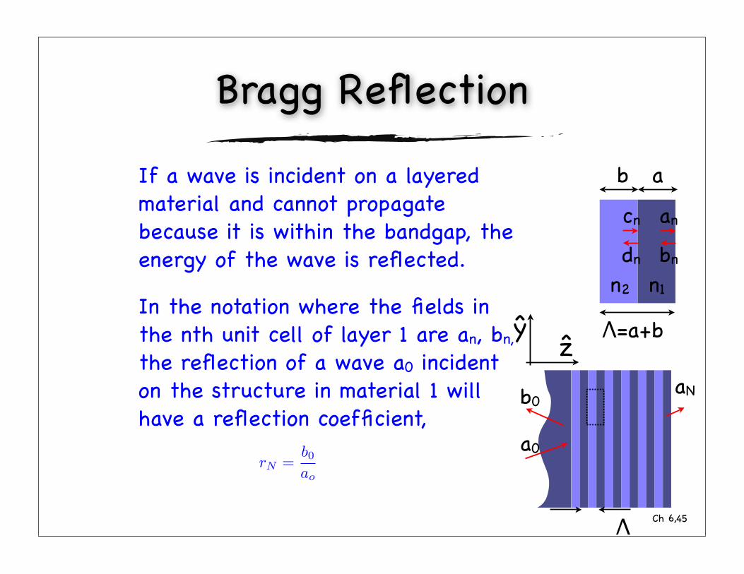
Bragg Reflection

If a wave is incident on a layered material and cannot propagate because it is within the bandgap, the energy of the wave is reflected.

In the notation where the fields in the nth unit cell of layer 1 are an, bn,

the reflection of a wave a0 incident on the structure in material 1 will have a reflection coefficient,

Λ

an

bn

cn

dn

n2 n1

Λ=a+b

ab

zy

aN

a0

b0

rN =b0

ao

45

Ch 6,

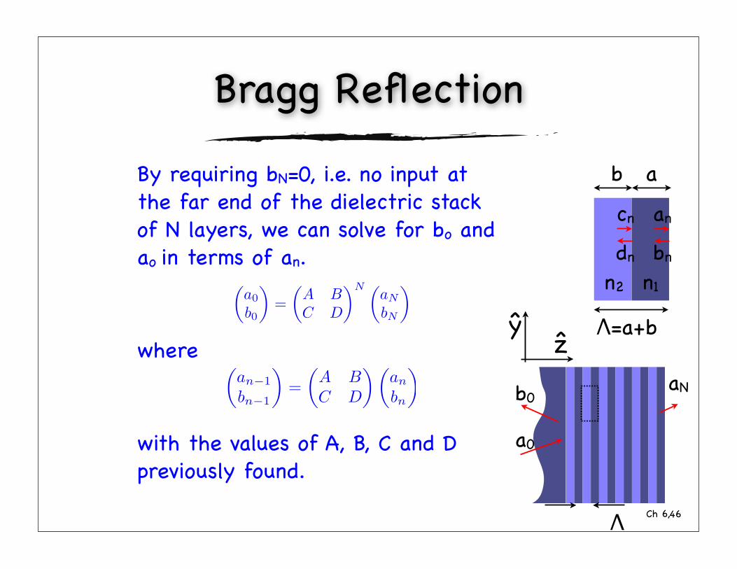
Bragg Reflection

By requiring bN=0, i.e. no input at the far end of the dielectric stack of N layers, we can solve for bo and ao in terms of an.

where

with the values of A, B, C and D previously found.

Λ

an

bn

cn

dn

n2 n1

Λ=a+b

ab

zy

aN

a0

b0

(a0

b0

)=

(A BC D

)N (aN

bN

)

(an−1

bn−1

)=

(A BC D

) (an

bn

)

46

Ch 6,

Bragg Reflection

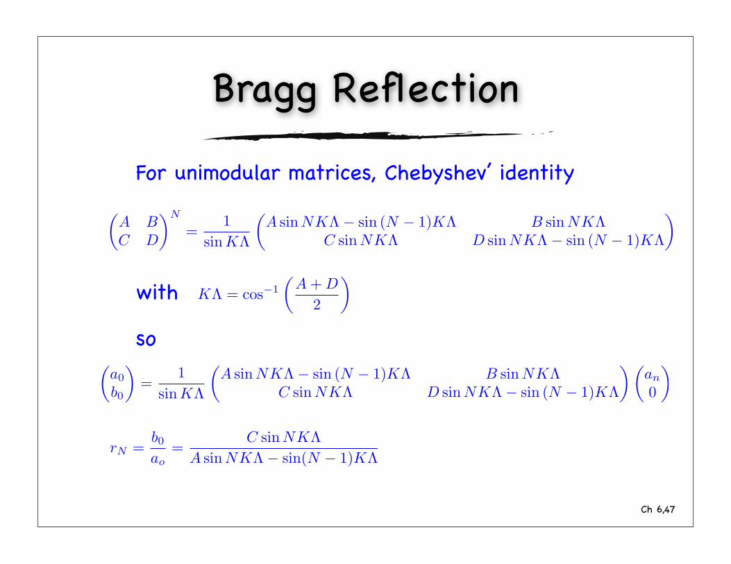
For unimodular matrices, Chebyshev’ identity

with

so

(A BC D

)N

=1

sinKΛ

(A sinNKΛ− sin (N − 1)KΛ B sinNKΛ

C sinNKΛ D sinNKΛ− sin (N − 1)KΛ

)

KΛ = cos−1

(A + D

2

)

(a0

b0

)=

1sinKΛ

(A sinNKΛ− sin (N − 1)KΛ B sinNKΛ

C sinNKΛ D sinNKΛ− sin (N − 1)KΛ

) (an

0

)

rN =b0

ao=

C sinNKΛA sinNKΛ− sin(N − 1)KΛ

47

Ch 6,

Structure Reflectivity in Air

Consider an infintesimal thickness of material 1 on top of the layered stucture. It has reflectivity ra1 on the air side (from air to material 1), and reflectivity rN on the structure side.

Ein Ec Et

Erl=0

andgiving

r,tr,t

so the reflectivity of the structure in air is

andEc = tEin − ra1rN Ec Er = ra1Ein + rNta1Ec

Ec =tEin

1 + ra1rNEr =

ra1 +

t2a1

1 + ra1rN

Ein

r =ra1 + rN

1 + ra1rN

48

Ch 6,

N=1 N=2

N=4 N=8

Spectral ReflectivitySpectral reflectivity RN at normal incidence of an N layer stack (quarter wave at ω0, nh=2.5, nl=1.5)

Rn = |rN |2 =∣∣∣∣

C sinNKΛA sinNKΛ− sin(N − 1)KΛ

∣∣∣∣2

49

Ch 6,

Summary

50

Ch 6,

References

Yariv & Yeh “Optical Waves in Crystals” chapter 6

http://www.tf.uni-kiel.de/matwis/amat/semi_en/kap_2/backbone/r2_1_4.html

51

Bloch waves and Bandgaps - San Jose State University

Documents

Transcript of Bloch waves and Bandgaps - San Jose State University