Bittensor: A Peer-to-Peer Intelligence Market

Yuma Rao

www.bittensor.com

Abstract

As with other commodities, markets could help us efficiently produce machineintelligence. We propose a market where intelligence is priced by other intelligencesystems peer-to-peer across the internet. Peers rank each other by training neuralnetworks which learn the value of their neighbors. Scores accumulate on a digitalledger where high ranking peers are monetarily rewarded with additional weightin the network. However, this form of peer-ranking is not resistant to collusion,which could disrupt the accuracy of the mechanism. The solution is a connectivity-based regularization which exponentially rewards trusted peers, making the systemresistant to collusion of up to 50 percent of the network weight. The result is acollectively run intelligence market which continual produces newly trained modelsand pays contributors who create information theoretic value.

The production of machine intelligence has come to rely almost entirely on a system of benchmarking,where machine learning models are trained to perform well on narrowly defined supervised problems.While this system works well for pushing the performance on these specific problems, the mechanismis weak in situations where the introduction of markets would enable it to excel. For example,intelligence is increasingly becoming un-tethered from specific objectives and becoming a commoditywhich is (1) expensively mined from data [1], (2) monetarily valuable [2], (3) transferable [3], and(4) generally useful [4]. Measuring its production with supervised objectives does not directly rewardthe commodity itself and causes the field to converge toward narrow specialists [5]. Moreover, theseobjectives (often measured in uni-dimensional metrics like accuracy) do not have the resolution toreward niche or legacy systems, thus what is not currently state of the art is lost. Ultimately, theproliferation of diverse intelligence systems is limited by the need to train large monolithic models tosucceed in a winner-take-all competition. Standalone engineers cannot directly monetize their workand what results is centralization where a small set of large corporations control access to the bestartificial intelligence [2].

A new commodity needs a new type of market1. This paper suggest a framework in which machineintelligence is measured by other intelligence systems. Models are ranked for informational produc-tion regardless of the subjective task or dataset used to train them. By changing the basis againstwhich machine intelligence is measured, (1) the market can reward intelligence which is applicableto a much larger set of objectives, (2) legacy systems can be monetized for their unique value, and(3) smaller diverse systems can find niches within a much higher resolution reward landscape. Thesolution is a network of computers that share representations with each other in a continuous andasynchronous fashion, peer-to-peer (P2P) across the internet. The constructed market uses a digitalledger to record ranks and to provide incentives to the peers in a decentralized manner. The chainmeasures trust, making it difficult for peers to attain rewards without providing value to the majority.Researchers can directly monetize machine intelligence work and consumers can directly purchase it.

1“The iron rule of nature is: you get what you reward for. If you want ants to come, you put sugar on thefloor.” - Charlie Munger

Preprint. Under review.

1 Model

We begin with an abstract definition of intelligence [6] in the form of a parameterized functiony = f(x) trained over a dataset D = [X,Y ] to minimize a loss L = ED[Q( y, f(x)) )]. Ournetwork is composed of n functions F = f0, ..., fj , ...fn, ’peers’ where each is holding zero or morenetwork weight S = [si] ’stake’ represented on a digital ledger. These functions, together with lossesand their proportion of stake, represent a stake-weighted machine learning objective

∑ni Li ∗ si.

f0 f1 f2 f3 f4 f5

L0 L1 L2 L3 L4 L5

D0 D1 D2 D3 D4 D5

Figure 1: Peer functions with losses Li and unique datasets Di.

Our goal is the distribution of stake to peers who have helped minimize this loss-objective (Figure-1). Our proposal achieves this through peer-ranking, where peers use the outputs of other peersF (x) = [f0(x)...fn(x)] as inputs to themselves f(F (x)) and learn a set of weights W = [wi,j ]where each wi,j is the locally calculated score attributed to the jth peer from the ith.

f0 f1 f2 f3 f4 f5

f0(x) f1(x) f2(x) f3(x) f4(x) f5(x)

y = f(F (x))

Figure 2: Inter-function connectivity.

f0 f1 f2 f3 f4 f5

w0,0 w1,1 w2,2 w3,3 w4,4 w5,5

w0,5, w5,0

Figure 3: Weight matrix.

Peers submit weight-updates to the digital ledger in the form of transactions which fill the blocksappended to the chain. Using these weights: (1) the digital ledger can compute ranks R = [ri] whichis the overall-score for each peer in the network and (2) proportionally inflate newly minted stake∆St = [∆si] to those peers. As inflation progresses, peers with significance to the overall objectiveare rewarded more and come to own a larger proportion of the network.

R = WT · S (1) St+1 = St + τ · R

||R||||S|| (2)

The immediate problem with this incentive system is that the computation of each weight wi,j inEquation (1) is non-auditable. It is not possible to enforce that weights be honestly reported withoutaccess to each function’s parameters, information we do not have on the distributed ledger. Instead,most if not all, participants will select weights which artificially increase their own rank – thisundermines the accuracy of the market.

2 Defining Consensus

Our solution begins with a convention: Messages from peer i to peer j are queued with respect tothe stake weight wi,j ∗ sj between them. Peers are thus persuaded to increase weights towards agame-theoretic equilibrium to better access the network. In the appendix we show how an informationtheoretic ranking arises at the system’s competitive equilibrium (See: appendix 12.1).

2

Figure 4: Similarity between a competitive peer-ranking and that found in coordinated environment.

However, competition provides only part of the solution: Peers with little competitive interest inattaining value from their neighbors may still collude to gain inflation without adding value to thenetwork. This is achieved by forming a ’cabal’, a set of one-or-more tightly connected peers whofalsely evaluate each other. Since there is no way to distinguish between weights which are correctlyset and those that are not, the default incentive mechanism rewards this behaviour.

f0 f1 f2 f3 f4 f5 f6 f7 f8 f9

HonestCabal

Figure 5: Disjoint cabal.

We can build protection against cabals through trust. Peers that are not trusted by the the majority ofthe network should attain less inflation. This way, assuming a cabal is smaller than the majority, itshould decay through time. To measure trust: (1) we compute a connectivity matrix C where cij isthe number of times in expectation peer i reaches peer j while traversing through the graph randomlyto some depth d and (2) use the tanh threshold function and cutoff κ to force each expectation onto−1 and 1.

C = tanh(

d∑k

(W −Wdg)k − κ) ≈

1 −1 −1 −1−1 1 −1 11 1 1 1−1 1 1 1

(3)

Note that, by this construction, (CT · S)i =∑nj sj · cj,i > 0 only for peers which are inwardly

connected to the majority. In conjunction with the sigmoid activation σ this score produces a newtrust based incentive method I 2 which exponentially rewards peers as trust increases. We write this,where ii ∈ Ii is the incentive for peer i, T is our trust vector T = σ(CT · S), and ranks R = WTSas follows:

I = WTS · σ(CTS) = R · T (4) St+1 = St + τ · I

||I||||S|| (5)

2Any function where x < 0→ δf(x)δx

> 1 works similarly for our purposes.

3

−0.4 −0.2 0 0.2 0.40

0.2

0.4

0.6

0.8

1

(CT · S)i

Ti

=σ

((CT·S

) i·1

0)

Figure 6: Sigmoid activation over our trust score Ti = σ(CT · S)i with temperature 10. (CT · S)i isnegative only when the proportion of stake which trusts peer i is less than 0.5 and positive otherwise.The sigmoid activation 1

1+e−x takes these values and produces an exponential scaling up to ourinflection point where a peer is connected to by the majority.

3 Reaching Consensus

Our new incentive function rewards connected peers, however, it may not solve the network problemif the honest network is disconnected. Loose, unused stake will detract from the weight of the honestnetwork in comparison to the cabal such that it may not gain enough inflation to overshadow itsadversary. Specifically, a dishonest graph will set weights optimally to ensure it is well connectedto itself, increasing the ranks of its members up to our inflection point at 0.5. It only needs attainenough inflation to compete with its largest competitor, not to entirety dominate the network.

δLδai

=

n∑k

rkci,k exp(tk)σ(tk)2

+wi,k(σ(tk)− 1

2)

tk =

k∑j

ajsjcj,k

(6)

Result: Gradient of peer iFunction gradienti(i,W,C, S,A) :

gradi = 0.0while k < in do

tk += A[j] ∗ S[j] ∗ C[j, k]endgradi += C[i, k] ∗R[k] ∗ etk ∗ σ(t+ k)2

gradi += W [i, k] ∗ (σ(tk)− 0.5)return gradi

end

Figure 7: Gradient computation for peer i with respect to a scaling factor ai and the chain’s lossfunction L . Note, for brevity, the stake values are assumed scaled si = si∑n

j sjand our sigmoid

temperature term is omitted.

To ensure that the honest graph can compete, we must force the bulk of stake to connect. We approachthis problem as a gradient-descent optimization with respect to a loss term L = −R · (T − 0.5)(Figure 7). Since the the cabal holds less than the majority of stake, the term (T − 0.5) is negativefor all of its peers. This way the loss can only be negative when the majority of incentives are beingdistributed to peers which are majority-trusted in the graph. The loss function L is optimized usinggradient decent with respect to a scaling factor over the stake A · S. As the blocks progress, we take

4

descent steps in the direction of our analytical gradient Equation (6), decreasing or increasing thescaling terms ai ∈ A ∈ [0, 1] towards our target point L < 0. (See: appendix 12.7)

In the worst case, the network is fully disconnected and we trivally minimize the chain’s loss atA = [0...0]. However, if the network contains a large connected component, the system convergestowards this dominant sub-graph. Self-interested peers can take the derivative of the consensusmechanism with respect to their scaling term ai. It makes sense for peers to ensure that their stake isnot scaled. At the same time, non-active peers will quickly lose staking power unless they continue tohelp consensus with outward connectivity. The result is a dual incentive which increases the inflationfor those that are well trusted and decreases the weight of disjoint stake.

4 Transactions and Token Inflation

A single token can be used to bootstrap the entire market. Inflation past this point is triggered bytransactions on the chain. Transaction fees can be pulled from the self-loop edge at each peer, thusthey are charged in the same token used as an incentive. Peers with no initial stake can still connectby solving a proof-of-work to make a subscription, or by having other peers subscribe them to thenetwork.

The proportion of inflation a peer may emit ei = τ(ai · si)∆t accumulates as time progresses. Thisway peers can always be sure to have enough fee to change their weights after a long enough wait.Peers with a large portion of stake can emit often with the fees being re-distributed back into theinflation pool. The emission is computationally cheap since the chain need only distribute the pendingemission outward and recompute trust scores when the weights are changed.

e0 = τ(c0 · s0)∆t

f0

f1 f3

f4 f5

f6 f7 f8

e 0∗ w

0,1

e0 ∗w0,3

e0 ∗ w0,4 e0 ∗ w0,5

e0 ∗w0,6

e 0∗w

0,7

e 0∗ w

0,8

Figure 8: Emission of new stake.

As inflation progresses, peers that make more transactions gain marginally more by maintaining theirconnectivity within the network. The need to continually submit transactions means that the largestsub-graph must perform work (i.e. monetary expense in the form of transactions) to continuallymaintain its dominance. Similar to Bitcoin, this limits the potential for long-term control-attacks onthe network: Only those that continue to work are rewarded with the highest proportion of inflation.

5 Tensor Standardization

A common encoding of inputs and outputs is required for the various model types and input typesto interact. The use of tensor modalities can be used to partition the network into disjoint graphs.At the beginning, the network can be seeded with a single modality TEXT, then expanded toinclude IMAGE, SPEECH, and TENSOR. Eventually, combinations of these modalities can be

5

added; for instance TEXT-IMAGE, to bridge the network into the multi-modality landscape. In-centives to connect modalities can be integrated with the same trust scaling suggested in section(2). Eventually, successful models should accept inputs from any modality and process them intoa useful representation. For consistency, we can use a standard output shape across the network[batch_size, sequence_dim, output_dim] similar to the common tensor-shapes produced by languageand image models – and extend this size as the network increase in complexity.

TEXT

IMAGE

TENSOR

f(x) [bs, seq, output]

[bs, seq]

[bs, seq, chans, rows, cols]

[bs, seq, input]

By working on abstract input classes we can ensure participants work towards a general multi-taskunderstanding [7]. Participants may use: (1) completely distinct computing substrates [8], (2) datasets[9], (3) models, and (4) strategies for maximizing their incentives in the market. It makes sense forpeers to work on unsupervised datasets where data is cheap and privacy not required.

6 Conditional Computation

As the network grows, outward bandwidth is likely to become a major bottleneck. The need to reducenetwork transfer and a method of selecting peers is required. Conditional computation can be usedwhere peers learn through gradient descent how to select and prune neighbors in the network. Forexample, a product key layer or a sparsely gated layer [10].

fi = fi(G(x)) (7)

G(x) =∑j

gj(x) ∗ fj(x) (8)

The conditional layer determines a sparse combination of peers to query for each example andmultiplicatively re-joins them, cutting outward bandwidth by querying only a small subset of peersfor each example. The method can drastically increase outward bandwidth [10] [11], allowing peersto communicate with many more neighbors in the graph. In essence, the layer acts as a trainable DNSlookup for peers based on inputs. Furthermore, being trainable with respect to the loss, it provides auseful proxy for the weights wi,j ∈W.

7 Knowledge Extraction

Dependence between functions ensures that models must stay online and cannot be run in production.Breaking this dependence can be achieved using distillation[6]: A compression and knowledgeextraction technique in which a smaller model – the student - mimics the behaviour of the remainingnetwork. The distillation layer is employed in conjunction with conditional computation (8) layer

6

where the student model learns to mimic the network using the cross-entropy (shown below as KL)between the logits produced by the gating network and the student’s predicted distribution [12].

distillation loss = KLD(dist(x), G(x)) (9)

Because the distilled model acts as a proxy for the network, models can be fully taken off-line andevaluated. Recursion through the network is also cut between components allowing for arbitrarynetwork graphs. If models go offline, their peers can use the distilled versions in-place. Private datacan be validated over the distilled models instead of querying the network. Eventually, componentscan fully disconnect from the network using the distilled models to do validation and inference offline.

fjfk fi

distk

DLi

Figure 9: Queries propagate to depth=1 before the distilled model is used.

8 Learning Weights

Our goal in this work is the production of a ranking r = [ri] over peers where score ri ∈ R representsa participant’s information-theoretic significance to the benchmark. Following LeCun and others[13; 14], it is reasonable to define this significance by equating it with the cost of removing each peerfrom the network. We can derive this score analytically where ∆F (x)i is a perturbation of the jth

peers’s inputs when the ith peer is removed from the network (Appendix 12.2):

ri ≈1

n

n∑j

∑x∈Dj

∆FT (x)i ·H(Qj(x)) ·∆F (x)i (10)

∆F (x)i = [0, ...0,−fi(x), 0, ...0]

Note, when the error function Qj is the twice-differentiable cross-entropy, then H(Qj) is its Fisher-information matrix, and ri ∈ R is suitably measured as each peer’s informational significance to thenetwork as a whole. However, information theoretic weights require the full Hessian of the error.In practice it is more reasonable to use a heuristic to propagate a contribution score from the errorfunction through to the inputs [14]. For instance, weights from the gating layer (Section 6) provide auseful differentiable proxy.

9 Running the Network

The steps to run a peer in the network are:

1. The peer defines its dataset Di, loss Li and parameterized function fi.2. At each training iteration, the peer conditionally broadcasts batches of examples from Di to

its peers x = [batch_size, sequence_length, input_size].3. The responses F (x) = [...fj(x)...] – each of common shape fj(x) =

[batch_size, sequence_length, output_size] – are joined using the gating function and usedas input to the local model fi.

7

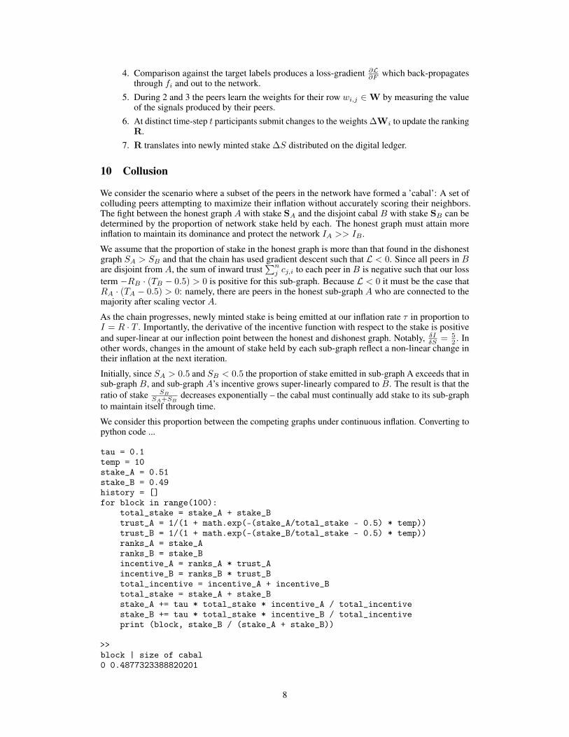
4. Comparison against the target labels produces a loss-gradient ∂L∂F which back-propagatesthrough fi and out to the network.

5. During 2 and 3 the peers learn the weights for their row wi,j ∈W by measuring the valueof the signals produced by their peers.

6. At distinct time-step t participants submit changes to the weights ∆Wi to update the rankingR.

7. R translates into newly minted stake ∆S distributed on the digital ledger.

10 Collusion

We consider the scenario where a subset of the peers in the network have formed a ’cabal’: A set ofcolluding peers attempting to maximize their inflation without accurately scoring their neighbors.The fight between the honest graph A with stake SA and the disjoint cabal B with stake SB can bedetermined by the proportion of network stake held by each. The honest graph must attain moreinflation to maintain its dominance and protect the network IA >> IB .

We assume that the proportion of stake in the honest graph is more than that found in the dishonestgraph SA > SB and that the chain has used gradient descent such that L < 0. Since all peers in Bare disjoint from A, the sum of inward trust

∑nj cj,i to each peer in B is negative such that our loss

term −RB · (TB − 0.5) > 0 is positive for this sub-graph. Because L < 0 it must be the case thatRA · (TA − 0.5) > 0: namely, there are peers in the honest sub-graph A who are connected to themajority after scaling vector A.

As the chain progresses, newly minted stake is being emitted at our inflation rate τ in proportion toI = R · T . Importantly, the derivative of the incentive function with respect to the stake is positiveand super-linear at our inflection point between the honest and dishonest graph. Notably, δIδS = 5

2 . Inother words, changes in the amount of stake held by each sub-graph reflect a non-linear change intheir inflation at the next iteration.

Initially, since SA > 0.5 and SB < 0.5 the proportion of stake emitted in sub-graph A exceeds that insub-graph B, and sub-graph A’s incentive grows super-linearly compared to B. The result is that theratio of stake SB

SA+SBdecreases exponentially – the cabal must continually add stake to its sub-graph

to maintain itself through time.

We consider this proportion between the competing graphs under continuous inflation. Converting topython code ...

tau = 0.1temp = 10stake_A = 0.51stake_B = 0.49history = []for block in range(100):

total_stake = stake_A + stake_Btrust_A = 1/(1 + math.exp(-(stake_A/total_stake - 0.5) * temp))trust_B = 1/(1 + math.exp(-(stake_B/total_stake - 0.5) * temp))ranks_A = stake_Aranks_B = stake_Bincentive_A = ranks_A * trust_Aincentive_B = ranks_B * trust_Btotal_incentive = incentive_A + incentive_Btotal_stake = stake_A + stake_Bstake_A += tau * total_stake * incentive_A / total_incentivestake_B += tau * total_stake * incentive_B / total_incentiveprint (block, stake_B / (stake_A + stake_B))

>>block | size of cabal0 0.4877323388820201

8

1 0.48495357843212472 0.48155115350942213 0.4773899015003984 0.47230934868432465 0.466122245746205876 0.458615908477375777 0.449558875400653768 0.438716437459128979 0.4258790087065162410 0.41090548935459825...90 0.000282725101061810191 0.0002571965388613131692 0.000233973024737379993 0.00021284643685656894 0.0001936274432965829395 0.000176143805861127496 0.0001602388369715894497 0.0001457699958275993698 0.0001326076112728088799 0.00012063371993464691

11 Conclusion

We have proposed an intelligence market which runs on a P2P network outside of a trusted environ-ment. Crucially, the benchmark measures performance as representational-knowledge productionusing other intelligence systems to determine its value. The fact that this can be done in a collaborativeand high-resolution manner suggests that the benchmark could provide a better reward mechanismfor the field in general.

To achieve this aim, the paper began with the definition of a P2P network composed of abstractlydefined intelligence models. We showed how this framework allowed us to produce a ranking foreach peer based on the cost to prune it from the network. Peers negotiated this score using a set ofweights on a digital ledger. However, the system was incomplete without mechanisms that preventedparticipants from forming dishonest sub-graphs.

To resolve this, we proposed an incentive scheme based on peer connectivity which exponentiallyrewarded peers for being trusted by a large portion of the network. This ensured that over timedishonest sub-graphs decay to irrelevance.

Following this, we showed (1) how peers reduced the network bandwidth by learning connectivityusing a differential layer and (2) how they could extract fully network-disconnected machine learningmodels to run in production. The result is an intelligence market which rewards participants forproducing knowledge and making it available to new learners in the system.

References[1] R. Schwartz, J. Dodge, N. A. Smith, and O. Etzioni, “Green ai,” 2019.

[2] OpenAI, “Openai licenses gpt-3 technology to microsoft,” OpenAI Blog, vol. 1, no. 1, p. 1, 2020.

[3] J. Devlin, M.-W. Chang, K. Lee, and K. Toutanova, “Bert: Pre-training of deep bidirectional transformersfor language understanding,” arXiv preprint arXiv:1810.04805, 2018.

[4] A. Radford, J. Wu, R. Child, D. Luan, D. Amodei, and I. Sutskever, “Language models are unsupervisedmultitask learners,” OpenAI Blog, vol. 1, no. 8, p. 9, 2019.

[5] F. Chollet, “On the measure of intelligence,” arXiv preprint arXiv:/1911.01547, 2019.

[6] G. Hinton, O. Vinyals, and J. Dean, “Distilling the knowledge in a neural network,” arXiv preprintarXiv:1503.02531, 2015.

9

[7] L. Kaiser, A. N. Gomez, N. Shazeer, A. Vaswani, N. Parmar, L. Jones, and J. Uszkoreit, “One model tolearn them all,” 2017.

[8] M. A. Nugent and T. W. Molter, “Cortical processing with thermodynamic-ram,” 2014.

[9] G. Lample and A. Conneau, “Cross-lingual language model pretraining,” 2019.

[10] N. Shazeer, A. Mirhoseini, K. Maziarz, A. Davis, Q. Le, G. Hinton, and J. Dean, “Outrageously largeneural networks: The sparsely-gated mixture-of-experts layer,” 2017.

[11] M. Riabinin and A. Gusev, “Learning@home: Crowdsourced training of large neural networks usingdecentralized mixture-of-experts,” arXiv preprint arXiv:/2002.04013, 2020.

[12] L. C. J. W. T. Sanh, Victor; Debut, “Distilbert, a distilled version of bert: smaller, faster, cheaper andlighter,” arXiv preprint arXiv:1910.01108, 2019.

[13] Y. LeCun, D. J. S, and S. S. A, “Optimal brain damage,” Advances in Neural Information ProcessingSystems 2 (NIPS), 1989.

[14] R. Yu, A. Li, C.-F. Chen, J.-H. Lai, V. I. Morariu, X. Han, M. Gao, C.-Y. Lin, and L. S. Davis, “Nisp:Pruning networks using neuron importance score propagation,” 2017.

[15] D. Balduzzi, W. M. Czarnecki, T. W. Anthony, I. M. Gemp, E. Hughes, J. Z. Leibo, G. Piliouras, andT. Graepel, “Smooth markets: A basic mechanism for organizing gradient-based learners,” 2020.

[16] P. Dütting, Z. Feng, H. Narasimhan, D. C. Parkes, and S. S. Ravindranath, “Optimal auctions through deeplearning,” 2017.

12 Appendix

12.1 Ranking Accuracy

We consider the accuracy of the ranking mechanism when peers make self interested updates to the weightson chain. The peers are under incentive pressure to both minimize their loss and stay connected within thelargest sub-graph. Since the mechanism is suitably mathematical we model each peer’s payoff function as adifferentiable utility function of the weights U(L(W))

Pi(W) = Ui(Li(W)) (11)

A peer’s utility term reflects that peers subjective interest in minimizing their loss U(L(W)). Since reducingthe magnitude of weights connecting this peer to others will decrease its ability to extract knowledge, we canmodel our utility function as a change in inputs. To model this change we use a shifted threshold i.e. inputs fromneighbors are masked when weights drop bellow the average set by other peers µj = ( 1

n)∑ni si ∗ wi,j which

in turn reflect a change in the loss function of peer i.

FW(x) = [f0(x) ∗ σ(si ∗ wi,0 − µ0), ..., fn(x) ∗ σ(si ∗ wi,n − µn)] (12)

σ =1

1 + e−xT

(13)

To derive the change in loss given a change in weights we use an input perturbation (FW − FW0) where W0 isthe initial choice of weights. The same perturbation equation seen Section 7 returns the change in loss under aHessian term H(L(F )) (see 12.3):

∂L

∂W=

∂

∂W

[(FW − FW0)T ·H(L(F )) · (FW − FW0)

](14)

We make a further linear assumption about the utility function Ui(W ) = α ·Li(W ) to give us a fully differentialfunction for a peer’s utility. This construction is a smooth market [15] where we can explore the competitiveequilibrium using gradient descent 3 with steps ∆Wi = ∂Pi

∂Wi.

Wt+1 = Wt + λ∆W (15)

3Making gradient steps in this game is a regret-free strategy (see 12.6) and achieves the best expected payoffin hindsight.

10

∆W =

[∂P0

∂w0; · · · ;

∂Pn∂wn

](16)

We evaluate the the accuracy of the peer ranking method by generating statistics from the above empiricalmodel. We first select mechanism parameters [λ, α, n] and generate an initial randomized network state [W0,S]with n random positive semi-definite n× n hessian terms [H] one for each peer. Given the initialization weapply the descent strategy (16) by computing the gradient terms from (14) and converge the system to theimplied equilibrium using a standard gradient descent toolkit. The discovered local minimum is the competitiveequilibrium where participants cannot vary from their choice of weights and stand to gain [16]. At this pointwe compute the competitive ranking R∗ and compare it to the idealized score R derived from the hessians asdiscussed in Section 7. We measure the difference between the two scores as a spearman-rho correlation andplot example trials bellow.

Figure 10: Correlations between the competitive rank and coordinated rank for α ∈ {1, 10, 25, 50}.We note that we see an increased relationship between the idealized rank and those discovered by themarket improves increasingly through the parameter α.

12.2 Deriving the idealized ranking

We approximate the change in the benchmark B =∑ni Li at a local minimum and under a perturbation

∆F (x)i = [...,−fi(x), ...] reflecting the removal of the ith peer.

∆B = B(F + ∆Fi)− B(F ) =

n∑i

Li(F + ∆Fi)− Li(F ) (17)

Li(F + ∆Fi)− Li(F ) ≈ ∂Li∂F·∆Fi +

1

2∆FTi ·H(Li) ·∆Fi +O(∆F 3

i ) +O(∆F 3i ) (18)

Equation (17) follows from the definition of the benchmark and Equation (18) follows from a Taylor series underthe perturbation ∆F (x)i. Note that the first term ∂Li

∂Fis zero at the local minimum and the higher order term

O(∆F 3i ) can be ignored for sufficiently small perturbations. These assumptions are also made by [13] and [14].

Note that Li is an expectation over the dataset Di, and all terms are evaluated at a point x so we have:

∆B ≈ 1

2

n∑i

∑x∈Di

∆FTi (x) ·H(Qi(x)) ·∆Fi(x) (19)

Here the hessian over the error function H(Qi(x)) and the summation over the dataset∑x∈Di

have beenappropriately substituted. The constant factor 1

2can be removed and this leaves our result.

12.3 Deriving the weight convergence game.

12.4 Theorem

For choice of Hessians H(L(F )) the network convergence-game can be described with the following linearrelationship between gradient terms:

∂P

∂W= α · ∂L

∂W+

∂r

∂W(20)

11

With the gradient of the loss:

∂L

∂W=

∂

∂W[(FW − FW0)T ·H(L(F )) · (FW − FW0)] (21)

12.5 Setup

We analyze the system by characterizing the behaviour of participants via their payoff in two terms:

1. The utility attached to that participant’s loss as a function of their weights is U(L(W)). U is assumedroughly linear for small change in the weight matrix, U(L) = α ∗ L, with ∂U

∂L = α, and α is assumedpositive and non-zero.

2. The network is converged to a local minimum in the inputs ∂L∂F

= 0.

From the payoff formulation in 6.3 we write:

P (W) = α · L(W) + r(W) (22)

Note, the utility function and emission were measured in similar units and so α is the price of each unit changein loss. The analysis just supposes such a score exists, not that it can be computed. Participants are selectingtheir weights by making gradient steps ∆Wi = ∂Pi

∂Wias to maximize their local payoff. For brevity we omit the

subscript i for the remainder of the analysis. Consider a Taylor expansion of the loss under a change ∆F in theinputs.

L(F + ∆F ) = L(F ) +∂L∂F

∆F +1

2∆F ·H(L(F )) ·∆F +O(∆F 3) (23)

The first linear term ∂L∂F

is zero at the assumed minimum and the higher order terms are removed for sufficientlysmall perturbations in F . We then perform a change of variable F = FW0 , and ∆F = FW1 −FW0 where W0

are the weights at the minimum and W1 are another choice such that FW0 and FW1 are those inputs maskedby W0 and W1 accordingly. Substituting this into Equation (29):

L(FW1) = L(FW0) +1

2(FW1 − FW0)T ·H(L(F )) · (FW1 − FW0) (24)

The function L(FW1) is simply an approximation of the loss for any choice of weights W1 given that thenetwork has already converged under W0. Finally, by the α-linear assumption of the utility we can attain thefollowing:

∂U

∂W= α · ∂L

∂W≈ α

2

∂

∂W[(FW − FW0)T ·H(L(F )) · (FW − FW0)] (25)

Note that we’ve dropped the subscript W1 for brevity, L(FW0)) is constant and therefore not depending on thechoice of weights, and the fraction 1

2can be safely subsumed into the unknown α. The remaining term ∂r

∂Wis

derivable via the ranking function in Section 1. This leaves the result:

∂P

∂W≈ α · ∂L

∂W+

∂R

∂W(26)

∂L

∂W=

∂

∂W[(FW − FW0)T ·H(L(F )) · (FW − FW0)] (27)

12.6 Deriving the ex-post zero-regret step.

Consider the system described above. A set of n peers are changing the weights in the ranking matrix Witeratively using gradient descent with learning rate λ. Wt+1 = Wt + λ∆W. Here, the change of weights is∆W = [∆w0, ...,∆wn] where each ∆wi is a change to a single row pushed by peer i. Each peer is attemptingto competitively maximize it’s payoff as a function of the weights Pi(W).

12

12.6.1 Definition

The ex-post regret for a single step is the maximum difference in loss between the chosen step ∆wi and allalternative ∆w∗i . The expected ex-post regret is this difference in expectation, where the expectation is takenover all choices ∆wj’s chosen by other participants [16].

rgti = E∆wj [max∆w∗

i

[Pi(∆w∗i )− Pi(∆wi)]] (28)

12.6.2 Theorem

For sufficiently small λ, the expected ex-post regret for strategy ∆wi = ∂P∂wi

is 0.

12.6.3 Proof

Consider Taylor’s theorem at the point W for the payoff function P under a change in weights W∗ =W+λ∆W. There exists a function h(W∗) such that in the limit as, W∗ →W we have the exact equivalence:

P (W∗) = P (W) +∂P

∂W(W∗ −W) + h(W∗) (29)

Let P (W∗) represent the payoff when the weight change of the ith row is ∆Wi = ∂P∂Wi

, and let P (W∗) beany other choice. Since λ→ 0, we have W∗ →W and by the definition of regret we can write:

rgti = E∆Wj [max∆W∗

i

[∂P

∂W(W∗ −W)− ∂P

∂W(W∗ −W)]] (30)

This follows by subtracting Equation (29) with choice W∗ and W∗. Next, substituting W∗ −W = −λ∆Wand expanding ∂P

∂W∆W = [ ∂P

∂W0∗∆W0, ...

∂P∂Wn

∗∆Wn] into the equation above leaves:

∂P

∂W(W· −W)− ∂P

∂W(W· −W) = λ(

∂P

∂Wi·∆W∗

i −∂P

∂Wi·∆Wi∗)+

λ

n∑j 6=i

(∂P

∂Wj·∆W∗

j +∂P

∂Wj·∆Wj∗)

(31)

The constant λ can be removed and the second term depends only on weights of other rows Wj 6=i. Since theseare independent and evenly distributed these can be removed under the expectation E∆Wj . He have:

rgti = E∆Wj [max∆W∗

i

[∂P

∂Wi·∆W∗

i −∂P

∂Wi·∆Wi∗]] (32)

Finally, we use the the fact that for vectors a, b and angle between them θ, the magnitude of the dot productis |a||b|cosθ. This is maximized when the vectors are parallel θ = 0 and cos(θ) = 1. In our case, wehave the maximum when ∆Wi = κ ∗ ∂P

∂Wifor some constant κ > 0. Thus P (∆W∗) is maximize when

∆W∗i = κ ∗ ∂P

∂Wi. Since P (∆W∗) = P (∆W∗) in the maximum, this proves the point.

12.7 Simulating the Loss Convergence

Bellow is python code for simulating the stake-convergence of a disjoint competing sub-graph against themajority graph.

import matplotlib.pyplot as pltfrom scipy.sparse import randomfrom sklearn.preprocessing import normalizeimport numpy as npnp.set_printoptions(precision=3, suppress=True)

def random_weight_matrix( n, density ):

13

rows = []for _ in range( n ):

row_i = random(1, n, density=density).A # Each row has density_Arow_i = normalize(row_i, axis=1, norm=’l1’) # Each row sums to 1.rows.append(row_i)assert np.shape(row_i)[1] == nassert np.isclose(np.sum(row_i), 1.0, 0.001)

W = np.concatenate(rows)assert np.shape(W)[0] == n and np.shape(W)[1] == nreturn W

def random_stake_vector( n ):S = np.random.uniform(0, 1, size=(n, 1))S = (S / S.sum())S = np.reshape(S, [1, n])S = np.transpose(S)return S

def sigmoid(x):return 1 / (1 + np.exp( -x ))

def get_gradient( n, W, R, S, A, C ):gradient = []for i in range(n):

grad_i = 0.0for k in range(n):

inner = 0.0for j in range(n):

inner += A[j] * S[j] * C[j, k]grad_i += C[i, k] * R[k] * np.exp(inner) * sigmoid(inner) * sigmoid(inner) + W[i, k] * (sigmoid(inner) - 0.5)

gradient.append(grad_i)

return np.concatenate(gradient)

def cabal_decay(nA:int = 5,nB:int = 100,n_blocks:int = 2000,tau:float = 0.01,learning_rate:float = 0.05

):r""" Measures the proportion of stake held by a disjoint sub-graph ’cabal’ as a function of steps.

Args:nA (int):

Number of peers in the honest graphnB (int):

Number of peers in the disjoint graphn_blocks (int):

Number of blocks to run.temperature (float):

temperature of the sigmoid activation function.tau (float):

stake inflation rate.learning_rate (float):

scaling term learning rate.

Returns:history (list(float)):

Dishonest graph proportion."""

n = nA + nB# Randomized Matrix of weights. We create the subgraphs by concatenating two disjoint

14

# and random square matrices.W = np.concatenate((

np.concatenate((random_weight_matrix(nA, 0.9), np.zeros((nA,nB)) ), axis=1),np.concatenate((np.zeros((nB,nA)), random_weight_matrix(nB, 0.9)), axis=1)),axis=0) ; print (’W \n’, W)

# Randomized Vector of stake.# Subgraph A gets 0.51 distributed across values 1->n_a.# Subgraph B gets 0.49 distributed across values 1->n_bS = np.concatenate((

random_stake_vector(nA)*0.51,random_stake_vector(nB)*0.49),axis=0) ; print (’S \n’, np.transpose(S))

# Scaling vector. A is multiplied by S before each iteration# to attain our scaled stake.A = np.ones(n) ; print (’A \n’, A)

# Matrix of connectivity. We use the true absorbing markov chain calculation# In practice this is too difficult to compute and opt for a depth d cut off.Wdiag = np.zeros((n,n))Wdiag[np.diag_indices_from(W)] = np.diag(W)Q = W - WdiagC = np.maximum(np.linalg.pinv(np.identity(n) - Q), np.zeros((n,n)))C = np.where(C > 0, 1, -1) ; print (’C \n’, C)

# Iterate through blockshistory = []for block in range(n_blocks):

# Scale the stake against our vector A.S_scaled = S * np.reshape(A, (n,1))#; print (’S * A \n’, S_scaled)

# Compute the ranks W^t S.R = np.matmul(np.transpose(W), S_scaled) / np.sum(S_scaled) #; print (’R \n’, R)

# Compute our trust scores sigmoid( (C^T S) * temperature )T = 1 /( 1 + np.exp(-np.matmul(np.transpose(C), S_scaled))) #; print (’T \n’, T)

# Compute our chain loss.loss = -np.dot(np.transpose(R), (T - 0.5) ) # ; print (’loss \n’, loss[0][0])

# Our loss is negative, so we emit more stake.if loss < 0.0:

# Compute our incentive function.I = R * T

# Distribute more stake.S = S + tau * (I/np.sum(I))

# Measure the size of our cabal.S_Honest = np.sum(S[:nA])S_Cabal = np.sum(S[nB:])ratio = S_Cabal / (S_Honest + S_Cabal)history.append(ratio)

# Our loss is positive, so we update our scaling terms.else:

# Compute the gradient of our scaling terms.grad = get_gradient( n, W, R, S, A, C ) #; print (’Grad \n’, grad)

# Update our scaling terms, being sure not to have negative values.A = np.minimum(np.maximum( A + learning_rate * grad, np.zeros_like(A) ), 1)

15

plt.plot(history)

cabal_decay()

16