Biologically and Physically-Based Rendering of Natural - DSpace
259
University of Calgary PRISM: University of Calgary's Digital Repository Graduate Studies Legacy Theses 1998 Biologically and physically-based rendering of natural scenes Baranoski, Gladimir V. Guimaraes Baranoski, G. V. (1998). Biologically and physically-based rendering of natural scenes (Unpublished doctoral thesis). University of Calgary, Calgary, AB. doi:10.11575/PRISM/18305 http://hdl.handle.net/1880/26230 doctoral thesis University of Calgary graduate students retain copyright ownership and moral rights for their thesis. You may use this material in any way that is permitted by the Copyright Act or through licensing that has been assigned to the document. For uses that are not allowable under copyright legislation or licensing, you are required to seek permission. Downloaded from PRISM: https://prism.ucalgary.ca
Transcript of Biologically and Physically-Based Rendering of Natural - DSpace
University of Calgary
PRISM: University of Calgary's Digital Repository
Graduate Studies Legacy Theses
1998
Biologically and physically-based rendering of natural
scenes
Baranoski, Gladimir V. Guimaraes
Baranoski, G. V. (1998). Biologically and physically-based rendering of natural scenes
(Unpublished doctoral thesis). University of Calgary, Calgary, AB. doi:10.11575/PRISM/18305
http://hdl.handle.net/1880/26230
doctoral thesis
University of Calgary graduate students retain copyright ownership and moral rights for their
thesis. You may use this material in any way that is permitted by the Copyright Act or through
licensing that has been assigned to the document. For uses that are not allowable under
copyright legislation or licensing, you are required to seek permission.
Downloaded from PRISM: https://prism.ucalgary.ca
THE UNTVERSITY OF C-4LGARY
Biologically and Physically-Based Rendering of Natural Scenes
Gladimir V. Guimarges Baranoski
-4 DISSERTATION
SUBblITTED TO THE F-4CULTY OF GRADUATE STUDIES
IN P-4RTIAL FULFILLMENT OF THE REQUIREMENTS FOR THE
DEGREE OF DOCTOR OF PHILOSOPW
DEPARTMENT OF COMPUTER SCIENCE
C-ALGARY, ALBERT-4
NOVEMBER, 1998
@ Gladimir V. Guimariies Baranoski 1998

National Library Bibliothèque nationale du Canada
Acquisitions and Acquisitions et Bibliographie Services services bibliographiques
395 WeIlington Street 395. rue Wellington OttawaON KIAON4 OttawaON KIAON4 Canada Canada
The author has granted a non- L'auteur a accordé une licence non exclusive licence dowing the exclusive permettant à la National Library of Canada to Bibliothèque nationale du Canada de reproduce, loan, distribute or seU reproduire, prêter, distn'buer ou copies of this thesis in microform, vendre des copies de cette thèse sous paper or electronic formats. la forme de microfiche/nlm, de
reproduction sur papier ou sur fomat électronique.
The author retains ownership of the L'auteur conserve la propiété du copyright in this thesis. Neither the droit d'auteur qui protège cette thèse. thesis nor substantial extracts fkom it Ni la thèse ni des extraits substantie1s may be p ~ t e d or otherwise de celle-ci ne doivent être imprimés reproduced without the author's ou autrement reproduits sans son permission. autorisation,
Abstract
Physicall-based rendering met hods represent the core of current realist ic image syn-
thesis frameworks. These methods, through a plausible simulation of the processes
of light propagation and interaction wit h ob jects, have contributed considerably to
the improvement of photorealistic rendering. The state of art research in this area
includes the simulation of natural phenomena and the incorporation of biological
aspects affecting light propagation in natural environrnents. The search for more
efficient rendering solutions is also of major interest for the rendering community.
In t his dissertation bio logically and p hysically- based models for light interaction
with plant leaves are presented. Moreover, since the light that reach a plant leaf may
be propagated directly from a light source or indirectly, due to multiple interactions
with other objects in the environment, global illumination issues are also addressed,
more specifically related to the radiosity method. This method is cornmoniy used to
account for the indirect mechanisms of light transfer. For this reason, faster solutions
for radiosity systems are also inwstigated in this dissertation.
The fundamental aspects of physically-based rendering as well as the main factors
affecting the light propagation by plant leaves are first presented to form a technical
background for the research that follows. -4n algorithmic reflectance and transmit-
tance model for plant tissue is presented next. Its accuracy is evaluated through
cornparisons with real measured data. For applications involving several foliar primi-
tives a nondeterministic algorithm for the reconstruction of isotropic reflectance and
transmittance functions is przsented as well as a simplified model for light interaction
with foliar tissues. Both models and the reconstruction dgonthm have a formulation
based on standard Monte Carlo methods.
The study of the spectral properties of the racliosity systems has not been exten-
sively explored by computer graphics and illuminating engineering researchers despite
its importance. These properties are investigated with the purpose of finding faster so-
lutions for radiosity problems. Besides t his theoretical study, t the Chebyshev method
for solving systems of linear equations is introduced to the rendering literature. This
met hod is particularly suitable for environments with high average reflectance and
occlusion commonly occurring in environmental design and remote sensing applica-
tions. Tests show that this method outperforms the iterative methods usually applied
to solve the radiosity systems under these conditions-
Finally. this dissertation closes with an outline of aspects that are worthy of
further investigation or extension. Among these aspects, the investigation of the
physical meaning of eigenvalues and eigenvectors in the global illumination context
is highlighted. P r e l i m i n ~ experiments are presented in the appendices.

Acknowledgement s
First of all. I rvould like to give my warmest thanks to twc =es. special women. My
mother? Eledi. me to say that she gave me %ings3. She's right; and 1 am deepb
indebted to her because of this. My wife, Adriane, knows better than anybody else
hom tough this pursuit of a Ph.D. degree nras. Her patience, confidence and love were
crucial in key moments of my program. This degree belongs to her too. Thanks a
lot!
My main achievements during this penod in North -4merica were not academic. 1
am talking about my kids, Patrïcia and Gabriel. So, 1 want to give my sincere thanks
to the friends who looked after them many times. Without their help in some difficult
moments, this joumey would have been much tougher.
1 am very grateful to Jon Rokne, my supervisor, for liis unconditional support
and friendship that made this journey nuch more enjoyable and fniitful. In fact, I
am not sure if 1 would have made to the other end of the tunnel without his heip. I
consider ~nyself very fortunate for having worked, during my graduate studies, with
supervisors who always consider the best interest of their students.
1 also enjoyed working with Randall Bramley and Peter Shirley a t Indiana Uni-
versity. They provided a valuable background for my doctorate research. While a t
Indiana, 1 also enjoyed the friendship and support of Younghee Lee7 Chih-Yi Chen,
-4lan Keahey, Shankar Swamy, Tom Loos, Rajesh Kamath ("Rom5rio") and Paulo
&f aciel.
1 am also grateful to all graphics jungle colleagues. My special thanks to Daniel
Dimian, whose fnendly conversations about sports, soccer, movies, and even cornputer
graphics, were much appreciated. My special thanks also to Radomir Mech and Dale
Brisinda, who many times listened to my complaints and gave me the opportunity to
release some steam.
1 want to thank rny defense cornmittee: Peter Ehlers, Przemyslaw Prusinkiewicz.
Brian Wyvill and Alain Fournier. Their comments and suggestions helped me to
improve the qua!ity of this dissertation.
I a h want to show rny appreciation to my k o c k defense" committee: Robson
Lemos. Mark Tigges, Dave Wilson, Jalal Kawash. Guangwu Su , Radek Kanvorvski
and Xikun Liang. Their confidence on the "eve of the battle" had a positive effect
on my own attitude.
Dunng graduate studies one often needs something to keep one's sanity. Soccer
and running mere my main "therapeutic" activities. 1 therefore thank my soccer
buddies and the Human Performance Laboratory (KPL) guys. My special thanks to
Marco Aureélio Vaz, who provided valuable logistics support during the early stages
of m ~ ; program and introduced me to the HPL relay team, and to the team's captain,
Joanne Archambauit.
Many people have provided valuable insights and feedback for the research pre-
sented in this dissertation: James -4rv0, Wayne Eberly, Richard Levy, Laslo Neu-
mann, Fred Baret, hf ichael Chelle, S tephane Jacquemoud, Rui Bastos, Zan Ashdown,
Manuel Menezes de Oliveira Xeto, Shirley Bray ... 1 thank al1 of them for their con-
tributions. My speciai thanks to Ken Girard of the Department of Biology for being
so generous with his time gronring the soybean plants used in this research. 1 am also
grateful to the Joint Research Center of the European Commission and the Advanced
Techniques Unit of the Space Applications Institute (Italy) for granting me access to
the LOPEX data set used in my experiments.
1 could not have performed my doctorate program without hanc ia l support.
Therefore, 1 want i;o express my sincere gratitude for the financial support provided
by the Brazilian National Council of Research (CNPq) , the Department of Computer
Science and the Faculty of Graduate Studies of the University of Calgary.

vii
3.4 Global Illumination Applications in Vegetation ........................... 53 3.5 Summary ............................................................ 56
Chapter 4 . The Algorithmic BDF Model for Plant Tissue 57 4.1 Outline of the Algorithmic BDF Model .................................. 58 4.2 Scattering Profile ...................................................... 60 4.3 .JLbsorption ............................................................ 63 4.4 Implementation Overview and S u m m a l of Parameters ................... 66 4.5 Testing Issues ........................................................ 67
4.5.1 Simulation of Devices for Measurement of Appearance ......... 68 .......................................... 45.2 Testing Parameters 73
4.6 Results and Discussion ................................................. 74 ............................................................. 4-7 Summary 79
Chapter 5 . A Nondeterministic Reconstruction Approach 81 5.1 The Reconstruction Approach .......................................... 82
1 Data Generation .................... .. ..................... 82 5-12 Reconstruction .............................................. 84 5.1.3 Searching ................................................... 85
5.2 Testing Parameters and Procedures ..................................... 87 5.3 Results and Discussion ................................................. 88 3.4 Summary ............................................................. 92
Chapter 6 . A Simpfified Model for Light Interaction with Plant Tissue 94 ............. 6.1 The Simplified Mode1 .................................. ,. 95
................... 6.2 Implernentation Overvietv and Summary of Parameters 97 6.3 Testing Issues ......................................................... 99 6.4 Results and Discussion ................................................ -102 6.5 Summary ............................................................ -109
Chapter 7 . Eigem.4 nalysis for Radiosity Systems 111 7.1 The Radiosity System of Linear Equations ............................... 112
7.1.1 Mathematical Formulation ................................... 112 7.1.2 Analysis in blatrix Terms .................................... I l 7
7.2 Solutions for Radiosity Systems ......................................... 120 7.2.1 The Gauss-Seidel Method ................................... -122 7.2.2 The Successive Overrelaxation Method ....................... 122
...... 7.2.3 The Progressive Rehement Method .. ................. -123 7.2.4 The Overshooting Approach ................................ -124
7.3 Eigenvalues and Eigenvectors ........................................... 125 7.3.1 Definition and Basic Properties ............................. -125
.......................... 7.3.2 Relationship with Iterative Methods 126 7.4 Proof that -111 Eigenvalues of the Radiosity Coefficient Matrk are Real and
Positive ............................................................... 127 ........................ 7.2 Eigenvalues Est imates for Radiosity Applications -129
7.6 Surnmary ............................................................. 130
Chapter 8 . Searching for Fast Solutions for Radiosity Systems 132 ................................................. 8.1 Residual Polynornials -135
........................................ 8.2 The Conjugate Gradient Method 136 8.2.1 Fundamentals ............................................... 136 5.2.2 Application to the Radiosity Problem ........................ -139
................................. 8 .2.3 Convergence Considerations -141 ................................................ 8.3 Chebyshev Polynomials 142
8.4 The Chebyshev Method ........................... .. ................... 143 ............................................... 8.4.1 Fundamentais 143
8.4.2 Application to the Radiosity Problem ......................... 145 8 - 4 3 Convergence Considerations .................................. 147
..................................... 8.5 Testing Parameters and Procedures 147 .................................. 8.5. 1 Performance Measurement -148
.................................................. 8.5.2 Test Cases 148 8.5.3 Convergence Checking ....................................... 150
......................................... 8.6 Testing Results and Discussion 151 .................................. 8.6.1 Steps of Iteration us Time -152
8.6.2 Effects of Reflectance and Occlusion on the Convergence ...... -157 ............................................................ 8.7 Summary -163
Chapter 9 . Conclusions 165 9.1 Summary of Contributions ............................................ -165 9.2 Further Research ..................................................... -171
References 175
Appendix A . Monte Carlo Techniques for Directional Sampling 201 ..................... Al Importance Sarnpling and Warping Transformations - 2 0 1
......................................... A.2 Probability Density Functions -203 A.3 Warping Functions .................................................... -206 A.4 Summary ............................................................. 208
Appendix B . Accuracy of Methods for Form Factor Computation 209 B.1 Impications of the Form Factor Numerical Errors ....................... -210 B.2 Statement of the ~Methods ............................................. -210
B.3 Cornparison Cnteria . . . . . . . . . . . . . . . . . . . . . . . . . . . . . . . . . . . . - - . - . - . . . - - - - . -212 B.4 Results . . . . . . - . - . . . . . . . . - . . . . . . . . - . . - - - . . - . . - . . - . - - - . . - - . - - - - - . . - . - - . -214 B.5 Sumrnary . . . . . . . . . . . . . . - - - . - - - - - - - - - . - - . . - . . - . - - . . . . . . . - - - . - - - . . - . . - . -218
Appendix C. Experiments with Eigenvectors 219 C.l Esperiments Set-Up . . . . . . . . . . . . . . . . . . . . . . . . . . . . . . . . . - . - . - - . . - . . - . - . . - 220 C.2 Mathematical Background.. . . . . . . . . . . . . . . . . . . . . . . . . . . . - . - - - - . . - . - - - . - - - 221 C.3 Eigenvectors Corresponding to the Smallest Eigenvalue of the Radiosity
373 Matrices . . . . . . . . . . . . . . . . . . . . . . . . . . . . . . . . . . . . . . . . . . . . . . . . . . . . . . . . . . . . . . . . C.4 Eigewectors Corresponding to the Largest Eigenvalue of the Radiosity
Uatrices . . . . . . . . . . . . . . . . . . . . . . . . . . . - . . . . . . . . . . . . . . - . . - . - - - . . . . . . - . . . . - 224 C.5 Eigenvectors Corresponding to the Largest Eigenvalue of the Symrnetric
Radiosity Matrices . . . . . . . . . . . . . . . . . - - - - - . . . . . . . . . - - . . . . . - - . . . . . . . . . . - . -227 (2.6 Eigenvectors Corresponding to the Smallest Eigenvalue of the Symrnetric
Radiosity Matrices . . . . . . . . . . . . . . . . . . . . . . . . . . . . . . . . . . . . . . . . - . - . - . . . . . . . -233 C.7 Discussion and Summary . . . . . . . . . . . . . . . . . - - . . . . . . . . . . - . . . - . . . . . . . . . . . . -235
Appendix D. Finding an Optimal Scding Parameter 237
Index
List of Tables
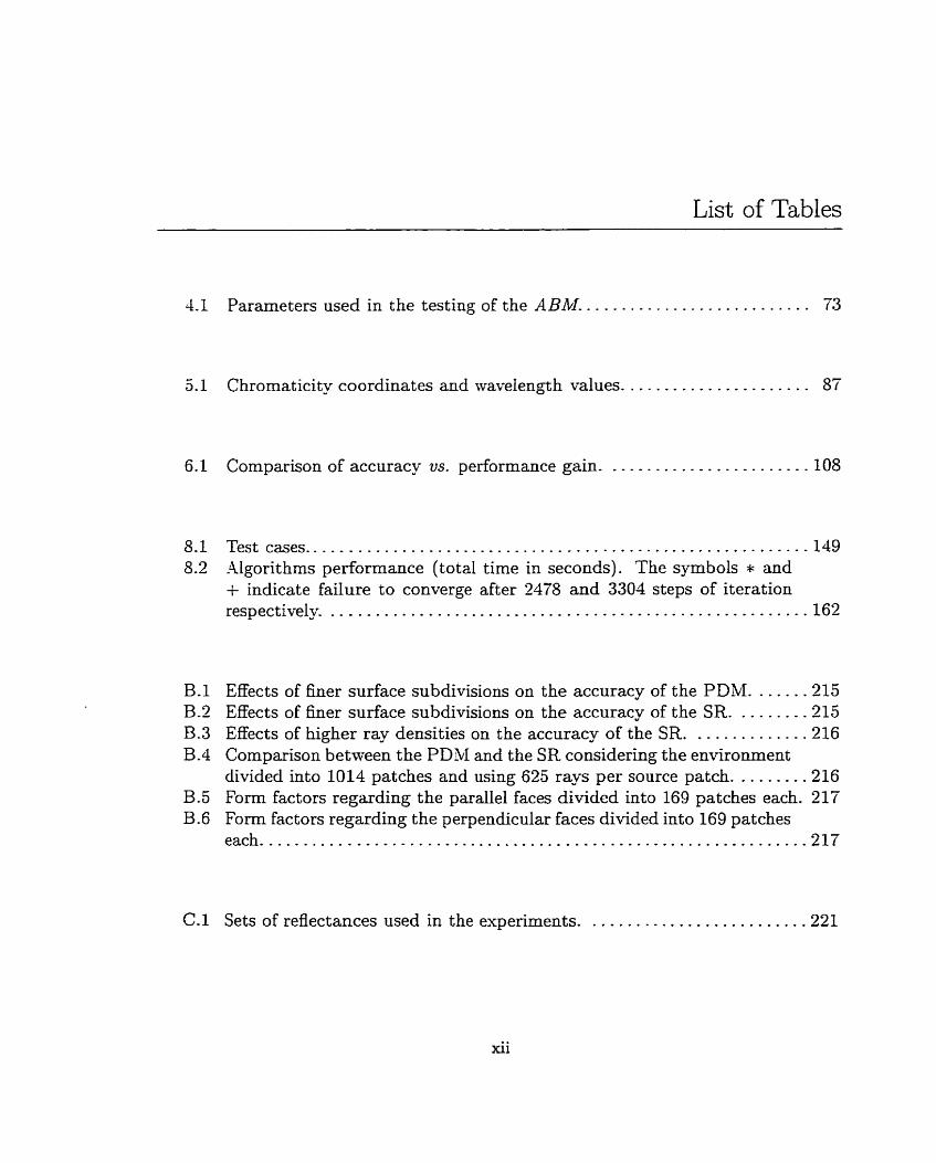
4.1 Parameters used in the testing of the ABM .......................... 73
1 Chromaticity coordinates and waveiength values ...................... 87
6.1 Cornparison of accuracy us . performance gain ........................ 108
.......................................................... 8.1 Test cases 149 5.2 Algorithms performance (total time in seconds) . The symbols * and
+ indicate failure to converge after 2478 and 3304 steps of iteration ....................................................... respectiveiy 162
B.l Effects of finer surface subdivisions on the accuracy of the PDM . . . . . . -215 B.2 Effects of finer surface subdivisions on the accuracy of the SR ........ -215 B.3 Effects of higher ray densities on the accuracy of the SR .............. 216 B.4 Cornparison between the PDM and the SR considering the environment
divided into 1014 patches and using 625 rays per source patch ........ -216 B.5 Form factors regarding the pardel faces divided into 169 patches each . 21'7 B.6 Form factors regarding the perpendicular faces divided into 169 patches
each ............................................................... 217
C.1 Sets of reflectances used in the experiments ......................... - 2 2 1
xii
List of Figures
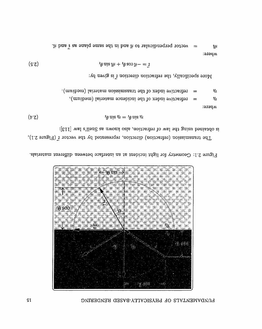
2.1 Geometry for light incident at an interface between different materials. 15 2.2 Reciprocity of the BDF. ............................................ 19 2.3 Loss of iight a t wavelength X in a medium of thickness h. ............. 22 2.4 Geometry for computing L, as an integral over d l the surfaces nrithin
the environment .................................................... 24 2.3 Geometry for computing L, in terms of al1 directions visible to a point
................................................................ x.. 25 2.6 a) Ideal diffuse and ideal specular distribution of reflected and trans-
rnitted light. b) General distributions of reflected and transmitted light. 26 ........................................... 2.7 Shadowing and masking. 33
3.1 T_vpical cross-section of foliar tissues. ................................ 40 3.2 -4rtist's conception of a typical epidermis tissue (Courtesy of Daniel
Dimian, The University of Calgary). ................................. 41 3.3 Cumes of reflectance and transmittance of a soybean leaf obtained
using the ABM (Chapter 4) a t a wavelength of 550nm and considering ...... the front (adaxial epidermis) of the leaf towards the Iight source. 44
4.1 Interfaces and tissues considered by the ABM. ....................... 59 4.2 Perturbations performed by the ABM on the rays distributions at the
four interfaces in the upwards and downwards directions of propagation considering the adaxial surface on the top and the abaxial surface on the bottom. a) Interface 1. b) Interface 2. c) Interface 3. d) Interface 4. 62
4.3 Mesophyll luop. a) Ray coming from outside interacts with interface 1. b) Refracted ray fIom interface 1 interacts with interface 2. c) Reffected ray from interface 2 interacts with interface 1. d) Ray coming from interface 3 interacts with interface 2. ........................... 63
4.4 Absorption spectra of chlorophylls e + b used in the testing of the ABM. 74
Cornparison of spectral curves of a soybean Ieaf computed with the ABM with measured spectral curves provided by L OPEX, for an angle of incidence of 8" and 1C16 rays. a) Absolute spectral reflectance. b) -- .................................... Absolute spectral transmit.tance. (3
Spectrophotometric curves of a soybean leaf obtained using the ABM and considering its front surface (adaxial surface) towards the light and its back surface (abaxial surface) towards the light, for an angle of incidence of 8" and 106 rays. a) Absolute spectral reflectance. b) Absolute spectral transmittance. .................................... 76 BDF of a soybean leaf a t a wavelength of 530nm (which corresponds approximately to the reflectance and transmittance peaks), for angles of incidence of lJO, 30" and 45", in the plane given by the incidence direction and the normal of the specimen, 107 rays, and the collecter sphere divided into 20 patches along its latitude and 40 patches along its longitude. .................................................. 77
Number of interactions per ray and per wavelength for 104 rays. a) Graph for zero to fifty interactions per ray, b) Zoom in of the region with high frequency of interactions per ray. .......................... 78
...... Collecter sphere and virtual goniophotorneter coordinate system. 83 Example of pre-processing on S. a) Original row. b) After sorting. c) The corresponding entries in U. .................................. 84 a) Example of mapping bom T to H. a) T's row. b) The corresponding row entries in H. c) A&er post-processing. ..........................- 86 Comparison of BDF curves a t wavelength of 608nm (red region) for a front lit specimen obtained using the ABM (solid lines) with curves obtained using the reconstruction approach (dotted lines). ............ 89 Comparison of BDF curves at wavelength of 551nm (green region) for a fiont lit specimen obtained using the ABM (solid lines) with curves obtained using the reconstruction approach (dotted lines). ........... 89 Cornparison of BDF curves a t wavelengtii of 455nm (blue region) for a front lit specimen obtained using the ABM (solid lines) wïth curves obtained usiog the reconstmction approach (dotted lines). ............ 90 Comparison of images obtained using: a) the ABM in-line, and b) the nondeterministic reconstruction approach. ........................... 90
xiv
Scattering distribution performed by the simplified model to represent the three components of a foliar specimen's SPF: a) surface reflectance
...................... b) subsurface reflectance and c) transmittance. 96 Graphs corresponding to the entries of the table of absolute spectral reflectances and transmittances for a soybean leaf.. .................. -100 Graphs corresponding to the entnes of the table of absolute spectral reflectances and trammittances for the veins of a soybean leaf. ....... -101 BDF curves for a front lit leaf obtained at the wavelengths associated with the RGB channels (Table 6.1)- a) and c ) Using the ABiW b) and cl) Using the simplified model. ..................................... -103 Top row: front lit leaves (1'' set) using the ABM (a) and the simplified model (b). Middle row: back lit leaves (Yd set) using the ABM (c) and the simplified model (d). Bottom row: Images with ambient light only (3rd set) and using the A BM (e) and the simplified model ( f ) . For d l three scenes we used cc = 0.01. ................................. -104 Convergence graphs for: a) lS' set, b) 2"d set and c) 3rd set, showing the percentage of ra-s that still need to be propagated after each depth of propagation. ................................................... -106 Number of rays propagated a t each depth of propagation for: a) lst set, b) Yd set and c) 3'd set.. ....................................... 107
.................. Geometry of the form factor between two patches.. -114 -4 typical radiosity coefficient matrix, i. e. present ing diagonal domi- nance and relative low density. ..................................... -118 An image generated using the radiosity method.. .................... -119 Sketch of a Sun and shade simulation for a building. ................. -121
Monic Chebyshev polynomials. ..................................... -143 Sketch of the test scene (face 3 is frontal). .......................... -149 Case A (p,,, = 0.24, 6 = 53%) with performance measured in steps of iteration ........................................................... 152 Case A (p., = 0.24, 6 = 53%) with performance measured in CPU tirne. ............................................................. 153 Case B (p,, = 0.46, 6 = 53%) with performance measured in steps of iteration. ......................................................... 154 Case B (p,,, = 0.46, 6 = 53%) with performance measured in CPU time. ............................................................. 155
Yumber of times that patches are selected by progressive refinement (PR) and overshootinq (FEDA) methods to shoot out radiosity in order to solve the system regarding test case E (p., = 0.ï88; b = 70%). Patches are sorted on ascending order of selection times. . . . . . . . . . . . . -156 Case C (p,, = 0.77, b = 53%) with performance measured in CPU time. ...........t..r.............-....-..-...-.................... 157 Case D (pu,, = 0.88, 6 = 53%) with performance measured in CPU time. ............................................................. 138 Case E (p,, = 0.78, b = 70%) with performance measured in CPU time. ............................................................. 159 Case F (puvg = 0.89, 6 = 70%) with performance measured in CPU time. ............................................................. 160 Eigenvalue distribution as the overall reflectance increases. . . . . . . . . . . . . 161 Chebyshev polynomials for scenes with different average reflectances. . . 161 Eigenvalue distribution as the density of the radiosity matriu decreases due to the increase on the level of occlusion in the scene.. . . . . . . . . . . . . -162
B.1 Geometry regarding a deterministic rnethod for f o m factor computa- tion using a Gaussian distribution of sample points. . . . . . . . . . . . . . . . . . - 2 1 1
B.2 Geornetry regarding a nondeterrninistic method for form factor com- putation using a random distribution of sample points. . . . . . . . . . . . . . . -212
B.3 Sketch of the test environment (face 3 is frontal). . . . . . . . . . . . . . . . . . . . . .213
C.1 Images corresponding to the solution (radiosity) vectors of the linear systems associated with: a) set 1 and b) set 2. . . . . . . . . . . . . . . . . . . . . . . .221
C.2 The directed graph of a square matrix K E C3x3- - - . . . . - - - - - - . . . . . . . . -223 C.3 Eigenvectors us of the matrices G associated with: a) set 1 and b) set 2.224 C.4 Images obtained using as solution vectors the eigenvectors of the
matrices G associated with: a) set 1 and b) set 2; and images obtained using as solution vectors the vectors of reflectances associated with: c) set 1 and d) set 2.. . . . . . . . . . . . . . . . . . . . . . . . . . . . . . . . . . . . . . . . . . . . . . . . . -225
6.5 Eigenvectors v~ of the matrices G associated with: a) set I and b) set 2.226 C.6 Images obtained using as solution vectors the eigenvectors u~ of the
matrices G associated with: a) set 1 and b) set 2. . . . . . . . . . . . . . . . . . . . -226 C.7 Eigenvectors u~ of the symmetric matrices GS associated with: a) set
1 and b) set 2. . . . . . . . . . . . . . . . . . . . . . . . . . . . . . . . . . . . . . . . . . + . . . . . . . . . . -227
C.8 Images obtained using as solution vectors the eigenvectors v~ of the matrices Gs associated with: a ) set 1 (mith 7 = 1.0): b) set 2 (with
......... y = 1.0): c) set 1 (with y = 2.2) and d) set 2 (wïth 7 = 2.2). -228 C.9 Zoom in of the cornponents of the eigenvectors u~ regarding the non
............ emitter patches and associated with a ) set 1 and b) set 2. .229 C.10 Images obtained using as solution vectors the adjusted versions of the
eigenvectors v~ regarding the matrices Gs associated with: a) set 1 (with y = 1.0): b) set 2 (with y = 1.0): c) set Z (with y = 2.2) and d) set 2 (mith = 2.2). .............................................. -230
C.11 Eigenvectors v~ of the s ~ i m e t r i c matrices Gs (with the reflectance of the emitter patches set to 0.9) associated with: a) set 1 and b) set 2. . -231
C.12 Images obtained using as solution vectors the eigenvectors v~ of the matrices Gs (with the reflectance of the emitter patches set to 0.9)
.. associated with: a) set 1 (with y = 2-2) and b) set 2 (with -f = 2.2). -232 C.13 Images obtained using as solution vectors the vectors L' associated
with: a) set 1 and b) set 2. ........................................ -232 C.14 Eigenvectors vs of the svymmetric matrices GS associated with: a) set
1 and b) set 2. .................................................... -233 C.15 Images obtained using as solution vectors the eigenvectors vs of the
matrices GS associated Mth: a) set 1 and b) set 2; and images obtained using as solution vectors the vectors P associated with: c) set 1 and d ) s e t 2............................................................234
xvii
CHAPTER 1
Introduction
Computer graphics involves the creation. storage. and manipulation of models and
synthetic images of objects. These images are used in areas as diverse as education,
science, engineering, medicine and entertainment [Xi]. Initially the main goal was
mostly to generate visually pleasing images. As the field developed this goal was
modified to include physical realism. Although there are applications, such as image-
for the entertainment industry, for which the aesthetic aspects are important, there
are also applications, such as illuminating engineering, for rvhich there is an increasing
demand for realistic images that can provide a physically truthful representation of
an object or an environment.
In order to add physical realism to a synthetic image the physical environment
has to be investigated. -4 substantial amount of computer graphics research has
been devoted to the simulation of light transport, i-e. the large-scale interaction of
light and matter [7], through rendering algorithms. In this context, the problem of
determining the appearance of an environment by simulating the transport of light
within it, which includes the problems of light emission, propagation, scattering and
absorption, is k n o m as global illumination [T, 2111.
This dissertation deals primarily with the research of physical models and numer-
ical methods for the simulation of light transport aiming a t realistic image synthesis
applications. In the following section a historical survey of the global illumination
methods used in computer graphics is presented. Then the interplay between the local
and global aspects of light transport is briefly discussed. Finally this chapter closes
with an outline of the theoretical and practical contributions and mith an overview
of the contents of this dissertation.
1.1 Historical Survey
The roots of the global illumination methods ased in computer graphics can be
traced back to the turn of the Iast centu~ïy- In 1900, Planck introduced the idea
that energy cornes only in discrete quantities, which is considered the beginning of
quantum mechanics, a revolutionary theory for submicroscopic phenornena [113]. In
1905: building on Planck's idea. Einstein post ulated t hat energy along an incident
bearn is quantized into small packets or "particles", later called photons [144] : whose
individual energy is given in terms of their wavelength and Planck's constant [86, 1131.
The concept of photons is fundamental for geometrical optics [113, 1491: also called
ray optics, which involves the study of the particle nature of light. -4lso in 1905,
Schuster [192] published a paper on radiation through a foggy atmosphere, and later,
in 1906, Schwarzschild published a paper on the equilibriurn of the Sun's atmosphere
[159]. These two astrophysical works are considered the beginning of the radiative
transfer theory [?. 45; 1791
In geometrical optics the large-scale behavior of light, such as reflection and re-
fraction, is described by assuming light to be cornposed of non-interacting rays, each
of them carryïng a certain amount of energy. The first algorithm for ray tracing was
presented by Appel [6]. Whitted 12361 extended this algonthm by incorporating many
of the principles of geometrical optics. This improved algonthm became the substrate
for a group of global illumination methods such as path tracing. This stochastic ray
tracing based method was introduced in the graphics literature by Kajiya [131] along
with a general physical framework for the global illumination problem known as the
rendering equation (further discussed in Section 2.4).
The radiative transfer theory combines principles of geometrical optics and ther-
modynamics to characterize the flow of radiant energy at scales large compared with
its wavelength and during time intervals large compared to its frequency [Tl. This
theory is the substrate of another group of global illumination methods, namely the
radiosity based methods (further discussed in Chapters 7 and 8)' introduced in the
computer graphics literature by Goral et al. [94]. The introduction of these methods is
considered the first step towards a more accurate approach to the global illumination
problem, known as physically-based rendering [136].
LYTRODUCTION 3
There are phenomena at the level of electromagaetism. such as interference: diffrac-
tion and polarization [113. 1981, that cannot be explained by geornetrical optics or ra-
diative transfer t h e o - These phenomena are addressed by physical optics [113, 1491,
mhich involves the study of the wave nature of light. Despite this limitation, geo-
metrical optics and radiative transfer t heory are the two levels of physical description
largely used in the simulation of visual phenomena aimed at image sy-nthesis applica-
tions. As mentioned by Glassner [86], this is a pragmatic choice, since the simulation
of phenomena such as interference, diffraction and polarization usually requires enor-
mous cornputational resources to produce results of significantly higher error fidelity
and complexity t han t hose attainable by geometrical optics. Models derived from
physical opt ics t heory [Il21 can be incorporated into a global illumination algorit hm
operating in the radiative transfer level [207]. When physical optics phenomena are
relevant for a given image sy-nthesis application they are usualIy handled as special
cases [164, 2141 or modeled using rendering algorithms based on geometrical optics
[219].
Ray tracing and radiosity based methods have been extended and combined to
solve different parts of the global illumination problem since their introduction in
cornputer graphies. R a - tracing based methods are particularly suit able for applica-
tions involving specular (mirror-like) reflections and refractions of light, but present a
high computational cost for applications involving multiple diffuse scatterings of light.
Radiosity methods, on the other hand, are particularly suitable to handle multiple
diffuse interactions of light? but present a high computational cost for handling the
high frequency signals associated with specular reflections and refractions of light.
The different approaches proposed to combine ray tracing and radiosity methods,
known as hybrid or rnuitipass rnethods, take advantage of the strengths of ray tracing
and radiosity while insuring that a single type of light transport is not accounted
for more than once [86]. For a comprehensive review of these methods the reader is
referred to the reference works by Cohen and Wallace [57], Sillion and Puech [211]
and Glassner [86]. Nthough these methods are resgonsible for the generation of very
realistic images, they usually do not accommodate materials that present properties
intermediate to those expected from ideal specular and ideal diffuse materials.
INTRODUCTION 4
It may be noteworthy to point out that, despite the latest achievements in render-
ing, it is not feasible. with the current technology. to give a viewer the same impression
Frorn a synthetic image as from Merving a real scene. Among the factors that preclude
this are aspects bey-ond the scope of this dissertation such as hardware limitations,
characteristics of the human visuai system and cognitive aspects of perception. -4s
pointed out by Shirley [198], these aspects have forced cornputer graphics researchers
to aim considerably lower than completely duplicating the perceptual response.
Nevertheless, the physical accuracy and the computationai trade-offs involved in
the processes of image synthesis are the dominant aspects of the current physicall-
based rendering research. Physical accuracy not only ensures the correctness of the
resulting images, but also makes the images predictive [7], a key requisite for prac-
t ical applications such as architectural and environmental design. Furt hermore, the
use of physical principles makes the rendering processes more intuitive, since- as
pointed out by Arvo [7], it is far easier to control a simulation using familiar physical
concepts than through arcane parameters. However, an accurate simulation of the
behavior of light in an environment, using current technology, is still computation-
ally espensive. Rather than sacrificing the quality of the synthetic images or simply
increasing the complesity of the rendering algorithms, the current trend in this field
is to push the boundaries of both accuracy and efficiency, and to extend the applica-
t ion of physically-based rendering met hods to materials with complex modes of light
interaction.
1.2 Interplay between Local and Global Illumination
In studying the core problem of physically-based rendering, global illumination, it
is often useful to distinguish its kvo components, direct and indirect illumination. By
direct illumination we mean the light from a light sourceL that arrives a t an object
without interacting with any other object dong its path [86]. By indirect illumination
me mean the light that undergoes at least one and possibly multiple interactions
rvith other objects before arriving at a given object. The rendering algorithms that
'Typical Iight sources or luminaires include thermal radiators, such as Barnes or incandescent
filaments, fluorescent bulbs and decaying phosphors [86].
INTRODUCTION
explicitly gather illumination information only from direct light sources are usually
called local illumination models and the rendering aigonthms that include estimates
of indirect illumination are usuaily called global illumination models [86].
Although these two terms local and global describe the extremes of a continuum,
one can not overlook the interplay behveen them. As pointed out by Fournier [76]?
the only may the light acts at the rendering level is locally. through intricate phenom-
ena, such as reffection. transmission and absorption of the incident light, which are
physically represented by reflectance and transmittance models (discussed further in
Section 2.6). In addition, considering that well-separated objects in an environment
can influence one another's appearance, either by blocking light in the case of direct
illumination; or by scattering light in the case of indirect illumination [ i l , direct and
indirect illumination are glo bally interconnect ed.
1.3 Outline of Contributions
In this dissertation original contributions to the study of local and global aspects
of light interaction wit h biological materials are made. These contributions range
from the development of reflectance and transmittance models for plants to the in-
troduct ion of faster solutions for radiosity systems.
The propagation2 to of light by most natural materials cannot be described as be-
ing purely specular or perfectly difise. Plants form a large class of natural materials
that fit this characteristic and for mhich there is a lack of physically and biologically-
based reflectance models aiming at rendering applications. Rather than proposing a
general purpose reflectance model, we intend to present reflectance models specifically
designed to take into account the biological factors that affect light propagation by
pIants.
The proposed models present different levels of complexity to increase their ef-
ficiency according to the rendering problem at hand. We consider this modeling
approach compatible with the current trends of seeking for practical solutions that
'Instead of explicitly mention reflection and transmission we will use the term propagation when
we refer to both processes in this dissertation.
INTRODUCTION 6
allow us to render materials with cornplex modes of reflection faster without under-
mining the accuracy of the simulations. In addition, it is also consistent with the
radiative transfer modeling approaches used in the study of vegetation as stated by
Asrar and Mynemi [12] :
We view the two types of modeling activities (i. e. simple us. detailed mod-
els) as cornplementary. Development of simple models could be pursued
either in parallel or as a follow-on to the development of more sophisti-
cated radiative transfer models.
The contributions to the global aspects of the simulation of light transport are the-
oretical and pract ical. As mentioned by -4rvo 171 : every global illumination problem
involves the solution of some linear system at some level. Moreover, several funda-
mental operators that anse in global illumination can be unifonnly approximated by
matrices; which suggests that functional analysis might be a useful tool for providing
a bet ter t heoretical foundation for global illumination [9]. This suggestion is followed
in this dissertation in the forrn of an investigation of the spectral properties of the
radiosity matris. We combine the results of this investigation wit h the introduction
of a numericd method which provides faster soiutions for radiosity systems associ-
ated with high average reflectance environments. Fie also discuss a more accurate
approach to evaluate the performance of the iterative solvers used in the radiosity
conte*.
The connection between the contributions of this dissertation to the local and
global aspects of the simulation of iight transport resides in the importance of radiosity
algorithms for radiative transfer in vegetation, which was appropriately expressed by
Asrar and Mynemi [12]:
The radiative transfer models that are currently in use for the study of
vegetative surfaces account only for the direct and diffuse components of
the incident solar energy, and the diffuse components that rnay emanate
from the vegetation and underlying soi1 surface. ... The concept of radios-
ity would permit accounting for al1 sources of radiation that may arrive a t
a surface independent of sensor position. ... The frontiers of research in
INTRODUCTION 7
this area are wide open and deserve the attention of the radiative transfer
modeling community concerned with the subject of vegetat ion canopies.
Sloreover, although the development and improvement of radiosity algorithms for
rendering applications mas not primarily aimed at organic materials, their use in the
field of radiative transfer in vegetation has grown rapidl- which is esemplified b -
related works not o d y in computer graphics [138: 1381, but a l s ~ in remote sensing
[35: 84, 891. As a result of this trend, the development of faster solutions for ra-
diosity systems has also become relevant to applications involving plant canopies: as
described in a recent paper by Chelle et al. [45].
1.4 Dissertation Overview
In this dissertation we will focus on the physical aspects of the light transport and
ive will describe light propagation in terms of geometrical optics. As mentioned in
Section 1.1, geometrical optics is usually used in cornputer graphics instead of physical
optics, since, from a practical point of view, it is more efficient to mode1 light as rays
rather than waves. We can think of a wave as just a ray with an energy, and the
wavelength of light, a physical optics parameter important for rendering applications,
can be included in geometrical optics by associating a wavelength with each ray
[198]. Furthermore, as pointed out by Shirley [198] and -4rvo [7], in many situations
physical optics effects are not visuaUy important, and do not dominate the scenes
that we commonly wish to simulate. For instance, the Light sources commonly used
in rendering applications are usually incoherent, and effects related to phase, such as
interference, are usually masked [7]. Also, diffraction phenornena are noticeable for
long wavelength radiation, but have a fairiy small effect for visible light [198].
In addition, in the experirnents presented in this dissertation we m-ill assume that
the energies of different wavelengths are decoupled. In other words, the energy asso-
ciated with some region of the space, or surface, at wavelength XI is independent of
the energy a t A2 [86]. We will also assume that objects within an environment ex-
change energy directly with no atmospheric attenuation. As mentioned by Arvo [ï],
atmospheric effects over tens of meters are insignificant under normal circumstances.
INTRODUCTION 8
Finall. participating media such as smoke. fog or water Nil1 not be addressed in this
dissertation,
Many of the techniques and results reported in this dissertation have been pre-
sented at cornputer graphics conferences [14- 15' 17' 18: 191. The main body of this
document is organized as folloms:
e Chapter 2 introduces relevant aspects of physical-based rendering t hat are
used t hroughout this dissertation. including the formulation of the light trans-
port yield by the rendering equation and the definition of important refiectance
and transmittance terms. -1 bnef survey of reflectance models used in corn-
puter graphics is also presented along n i th an ovenriew of global illumination
applications aimed at vegetation.
Chapter 3 presents the main factors affecting the interaction of light with plant
tissues, with a particular emphasis to leaves since they are the most important
plant surface interacting with light. An o v e ~ e w of the most important re-
flectance models for plants, mostly oriented to remote sensing applications, is
also presented. .Ut hough the requirements are different in computer graphics,
sorne of the intuitive concepts used in remote sensing models can be incorpo-
rated into models aimed at image synthesis applications.
Chapter 4 introduces a new algorithmic reflectance and transmittance mode1
for plant tissue aiming at image synthesis applications. The mode1 accounts
for the three components of light propagation in plant tissues: namely surface
reflectance: subsurface refiectance and transmittance, and rnechanisms of Light
absorption by pigments present in these tissues. Its design is based on the
available biological information. The model is controlled by a small number of
biologically meaningful parameters, and its formulation is based on standard
Monte Car10 techniques. The spectral curves of reflectance and transmittance
computed using the model are compared with measured curves ftom actual ex-
periments for real specimens. The formulation and techniques used to simulate
the virtual measurement devices used in the testing of the models proposed in
Chapters 4 to 6 are also presented in this chapter.
INTRODUCTION 9
Chapter 5 introduces a nondeterministic reconstruction algorithm for isotropic
reflectance and transmittance functions that can be used as an alternative for
deterministic approaches, such as spherical harrnonics [44, 2071 or wavelets
[X. 139, 140. 141: 2351: in applications involving isotropic materials. This al-
gorithm. also based on standard Monte Carlo methods, is general enough to be
not only appiied to the rendering of plants, but also to access arbitrary isotropic
reflectance and transmit tance functions. The reconstructed spectral curves ob-
tained through this algorithm are compared with spectral curves provided by
the model introduced in Chapter 4 in order to determine their accuracy-
Chapter 6 introduces a simplified model for light interaction with plant tissue
aiming at applications demanding higher performance. It accounts for the main
biological characteristics of these materials needed to preserve their rendering
quality, while avoiding undue complexity in order to increase their rendering
efficiency. The model's formulation is also based on Monte Carlo techniques,
and it can be incorporated into global illumination frameworks nithout a signif-
icant computational overhead. Its accuracy and performance is also examined
through cornparisons with the mode1 introduced in Chapter 4.
Chapter 7 discusses some important characteristics of the radiosity system of
linear equations and presents tools used in the investigation of its spectral prop-
erties. Particular emphasis is given to the definition and basic properties of the
eigenvalues and eigenvectors of the system along with their relationship to the
iterative methods used to solve the radiosity system. The major original con-
tribution introduced in this chapter is the analytical proof that al1 of the eigen-
values of the radiosity matrix are real and positive. This fact, among other
implications, permits the computation of tight estimates for the eigeuvalues
of the radiosity matrix, which are used to obtain faster solutions for radiosity
systems.
Chapter 8 introduces a numerical method to the graphics literature that con-
verges faster than the methods usually used in the radiosity problems associated
with environments with high average reflectance. We compare the performance
INTRODUCTION 10
of this method to other iterative solvers. and show that the performance eval-
uation approach based on a small nuaber of iterations. as opposed to small
amounts of time, commonly used in this area of research. can lead to incorrect
conclusions. We also show numerically the important relationship between the
characteristics of a given environment; such as average reflectance and level of
occlusion. and the spectral characteristics of the corresponding radiosity matrk.
We focus this discussion on the impact of this relationship on the convergence
of the iterative methods used to solve the radiosity system.
Finally? Chapter 9 summarizes the results and main contributions of this disser-
tation. A list of open questions is also presented along with possible directions
for future research.
The references and appendices follow the main body of this document. The ap-
pendices are organized as follows:
Appendix A presents some fundamental Monte Carlo definitions and techniques
used in this research as well as the concise derivation of functions used to gen-
erate scattered directions in rendering applications.
Appendiu B compares a deterministic method for form factor computation with
a nondeterministic one. This cornparison is focused on their numerical accuracy
regarding selected geometries, using the corresponding analytical form factors
as accuracy standards.
Appendiv C shows some interesting features of using the eigenvectors of the
radiosity matrix as solution vectors in graphics settings. The information gat h-
ered from these experiments is expected to contribute to the understanding of
physical meaning of the eigenvectors in the radiative transfer context, which, in
turn, may lead to faster solutions for global illumination problems.
Finally, AppendLu D proposes a parameter to scale the eigenvector correspond-
ing to the largest eigenvalue of the symmetric radiosity matrix. The purpose
of this scding operation is to use the resulting scaled eigenvector as an initial

INTRODUCTION 11
approximation for the solution vector of a radiosity system. The use of such an
initial approximation may also result in faster solutions for global illumination
problems, particularly t hose associated wit h radiosity systems.
Fundament als of P hysicdly-Based Rendering
In this chapter we will concentrate on the fundamental aspects of physicdy-based
rendering that will be used throughout this dissertation. Physically-based rendering
involves simulating the behavior of light, starting from luminaires, i. e. area light
sources, trav-eling through the environment, interacting with different objects, and
finally reaching the viewer. Reflect ance and t ransmittance models are used to describe
how the light interacts with different objects. These models must satis- certain
physical requirements to avoid excluding important physical effects and to maint ain
the energy consistency needed for global illumination calculations [235]. These issues
Mil also be examined in this chapter.
The sections of this chapter are organized as follows:
Section 2.1 presents basic laws of optics airning a t rendering applications.
Section 2.2 describes important spectral radiometric terms along with their
properties.
Section 2.3 presents the laws that describe the absorption of transmitted light
in homogeneous materials.
Section 2.4 outlines the basic formulation of light transport yield by the render-
ing equation.
Section 2.5 presents the basic mechanisms of light transfer, the tenninology used
to describe the reflective and refractive behavior of the surfaces and a notation
proposed by Heckbert [117] to represent these mechanisms.
FUNDA-MENTALS OF PHYSICALLY-BASED RENDERING 13
Section 2.6 introduces a concise overview of reflectance and transrnittance mod-
eIs used in cornputer graphics.
Final13 Section 2.7 summarizes the contents of this chapter.
2.1 Basic Optics
Throughout t his dissertation we will use the following terminology suggested by
Meyer-Arendt [Z61]. Terms ending in -ion, such as reflection, transmission and ab-
sorption, describe a process. Tenns ending in -ivity, such as reflectivity, transmissivity
and absorptivity, refer to a general property of a material. Terms ending in -ance,
such as reflectance, transmittance or absorptance, refer to properties of a given object
or surface..
Reflection is the process in which Iight a t a specific wwelength incident on a
material is propagated outward by the material without a change in wavelength.
Similarly, transmis~ion is the process in which light at a specific wavelength incident
on the interface between materials passes through the interface and into the other
material without a change in wavelength [86].
Hall [103] suggested that reflection and transmission can be broken into two com-
ponents, a coherent component and an incoherent or scattered component [%3]. The
coherent component is reflected using the law of reflection and transmitted using
the law of refraction, which are described later. The incoherent component is re-
flected and transmit ted in al1 directions based upon a statistical probability function
associated wit h surface properties ( Appendix A).
Absorption is a general term for the process by which the Iight incident on a
material is converted to another form of energy, usually to heat. Al1 of the incident
light is accounted for by the processes of reflection, transmission and absorption [5].
The reflection and transmission (refraction') of light at the smooth surfaces of
pure materials is described by the Fresnel equations [86, 113, 1981. Before getting to
LRc?fraction, or the coherent component of transmission, can be defined as the bending or the
change in the direction of the light rays as they pass kom one medium to another [122]. This bending
is deterrnined by the change in the velocity of propagation associated with the different indexes of refraction of the media [71].
FUNDAlZ/IENTALS OF PHYSICALLY-BASED RENDEFUNG 14
the specifics of the Fresnel equations. ho~vever~ we shall review some relevant physical
parameters, definitions and laws.
Materials such as conductors (metals) : semi-conduct ors and dielectrics are charac-
terized by their complex index of refraction, :V(X), which is composed of a real and an
imaginal term. The real term corresponds to the real index of refraction (refractive
indes: for short). which measures how much an electromagnetic wave slows don711 rel-
ative to its speed in vacuum [86]. The imaginary terni corresponds to the extinction
coefficient. mhich represents hom e a s i - an electromagnet ic wave can penetrate into
the medium [86]. The resulting expression for N(X) is given bp-:
where:
X = wavelengt h,
77 = real index of refraction as a function of A:
P = extinction coefficient as a function of A,
j = imagina. unit ( j = m) . Semi-conductors are conductors tvit h a small extinction coefficient. Dielectrics are
essentially non-conductors whose extinction coeficient is by definition zero [198]. For
notational simplicity, we will remove the esplicit dependency on X in the remaining
equations presented in this section.
The reflection direction, represented by the vector 7 (Figure Tl) , for light incident
at an interface is obtained using the law of reflection [1l3]. This states that the angle
of the reflection direction, O,, is equal to the angle of incidence, Bi, and d l be in
the same plane as the incident direction, represented by the vector z, and the surface
normal, represented by the vector 2
Considering the geometry described in Figure 2.1 and applying the law of reflection
stated above, the reflection direction, r', is given by:
FUNDAMENTALS O F PHYSICALLY-BASED RENDERING 16
Equation 2.5 can be erpanded to yield the expression presented by Heckbert [114]:
i= [-:(Te 5) - d=] 6+ ZT rit (2.6)
The incident rays are not only reflected and/or transmitted (refracted) at an
interface between dielectrics, but also attenuated. This attenuation is given by the
Fresnel coefficients for reflection and transmission (refraction), which are cornputed
through the Fresnel equations. For a complete derivation of these equations, the
reader is referred to the texts by Hecht and Zajac [Il31 and Glassner [86]. The Fresnel
equations for a smooth interface between two dielectrics ( p = 0) can be simplified to
the following expressions collected by Kajiya [130]:
In the previous equations RL and Ril are the Fresnel coefficients for reflection of
light polarized in directions perpendicular to (1) and parallel (11) to the interface.
Similady, TL and TiI are the Fresnel coefficients for transmission (refraction) of light
polarized in directions perpendicular to (1) and parallel (II) to the interface.
The Fresnel coefficient for reflection, or reflectivity [161], R, for polarized light is
the weighted sum of the polarized components, in which the weights must to sum
to unity [86]. In this dissertation we are interested in the Fresnel coefficients for
unpolarïzed light. In this case, the Fresnel coefficient for reflection is simply the
average of the two coefficients RL and RI,. Then, the equation used to cornpute this
FUNDAMENTALS OF PHYSICALLY-BASED RENDEFUNG
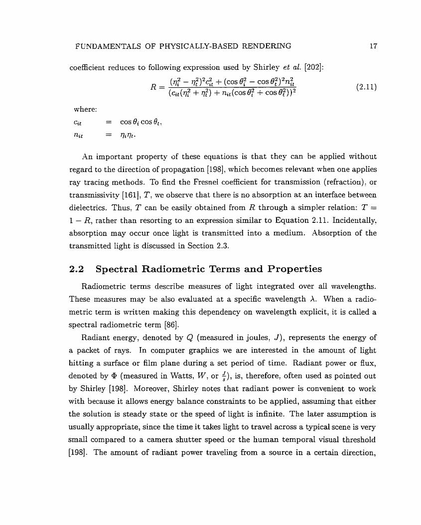
coefficient reduces to following expression used by Shirley et al. [202]:
($ - $ ) 2 c f t + (COS 0; - cos R =
(Q (7: + 7:) + nit (COS 0; + cos 07) )2
where:
ctt = COS Oi COS et: nit - - q'i 7it -
An important property of these equations is that they can be applied without
regard to the direction of propagation [198], which becomes relevant when one applies
ray tracing methods. To find the Fresnel coefficient for transmission (refraction), or
transmissivity [161], T: Rie observe that there is no absorption a t an interface between
dielectrics. Thus: T can be easily obtained from R through a simpler relation: T =
1 - R, rather than resorting to an expression similar to Equation 2.11. Incidentally?
absorption may occur once light is transmitted into a medium. Absorption of the
transrnitted Iight is discussed in Section 2.3.
2.2 Spectral Radiometric Terms and Properties
Radiometric terms describe measures of light integrated over al1 wavelengths.
These measures may be also evaluated at a specific wavelength A. When a radio-
metric term is written making this dependency on wavelength explicit, it is called a
spectral radiometric term [86].
Radiant energy, denoted by Q (measured in joules, J), represents the energy of
a packet of rays. In computer graphics we are interested in the amount of light
hitting a surface or film plane during a set period of tirne. Radiant power or flux,
denoted by Q (measured in Watts, W y or t), is, therefore, often used as pointed out
by Shirley [198!. Moreover, Shirley notes that radiant power is convenient to work
with because it allows energy balance constraints to be applied, assuming that either
the solution is steady state or the speed of light is infinite. The later assumption is
usually appropriate, since the tirne i t takes light to travel across a typical scene is very
small compared to a camera shutter speed or the human temporal visual threshold
[198]. The amount of radiant power traveling from a source in a certain direction,
FUNDh'IfLEINTALS OF PHYSICALLY-BASED RENDERING 18
per unit of solid angle2, is called the radiant intensity and denoted by I (measured
The underlying purpose of the rendering process is to determine the colors of the
surfaces mithin an environment. The color of a given surface d l depend on how much
light is ernitted. reflected? absorbed and transmitted by the surface. Since radiant
intensity depends on the area of the light source, it is not convenient to approximate
color, which is independent of surface area. As pointed out by Shirley [198], the
radiometric quantity that more closely approximates the color of a surface, through
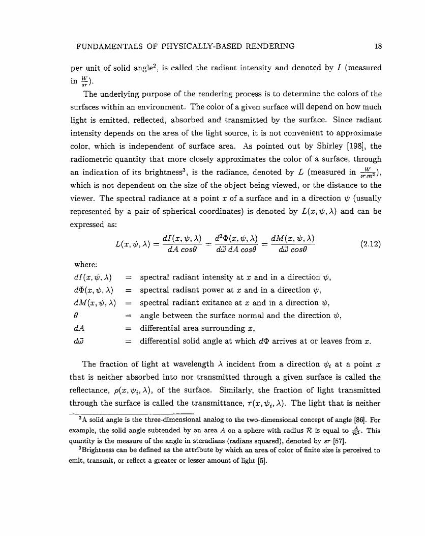
an indication of its brightness3, is the radiance, denoted by L (measured in 5): which is not dependent on the size of the object being viewed, or the distance to the
viem-er. The spectral radiance at a point x of a surface and in a direction 11i (usually
represented by a pair of spherical coordinates) is denoted by L(x, ILJ, A) and can be
espressed as:
where:
d i ( x , A) = spectral radiant intensity at x and in a direction Si,
( x , A) = spectral radiant power at x and in a direction Si,
d ( x A) = spectral radiant exitance at x and in a direction d~,
6 = angle between the surface normal and the direction @,
d A = differential area surrounding x,
dc5 = differential solid angle at which d@ arrives a t or leaves from x.
The fraction of light at wavelength X incident Tom a direction a t a point x
that is neither absorbed into nor transmitted through a given surface is called the
reflectance, p(x, Qi; A), of the surface. Similarly, the fraction of light transmitted
through the surface is called the transmittance, ~ ( x , Gi7 A). The light that is neither
?A solid angle is the three-dimensional analog to the two-dimensional concept of angle [86]. For
ewarnple, the solid angle subtended by an area A on a sphere with radius R is equal to &. This
quantitÿ is the rneasure of the angle in steradians (radians squared), denoted by sr [57]. 3B~ghtness can be defined as the attt-ibute by which an area of color of finite size is perceived to
emit, transmit, or reflect a greater or lesser amount of light [5].
FC'NDAMENTALS OF PHYSICALLY-BASED RENDERING 19
refiected nor transmitted by the surface is absorbed. The parameter that describes the
amount of absorbed light is absorptance [5 ] . The sum of the reflectance, transmittance
and absorptance is one.
The reflectance and the transmittance do not describe the distribution of the
reflected and transmitted light. The bidirectional rehctance distribution function
( B R D F ) , f,: and the bidirectional transmittance function (BTDF)? ft7 are used to
overcome this limitation. -4s suggested by Glassner [86], these functions can be com-
bined into the bidirectional surface-scattering distribution function ( B S S D F , or simplÿ
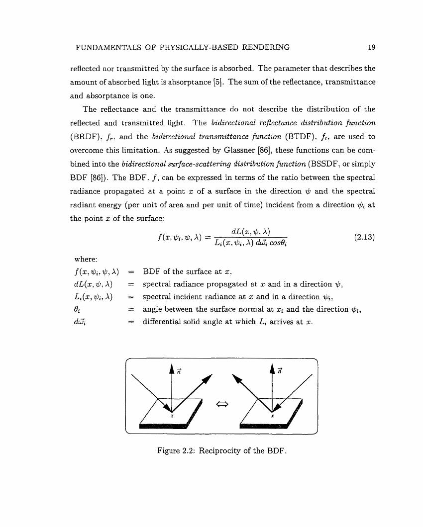
BDF [86]). The BDF: f , can be expressed in terms of the ratio between the spectral
radiance propagated a t a point x of a surface in the direction + and the spectral
radiant energy (per unit of area and per unit of time) incident from a direction a!+ at
the point x of the surface:
where:
( x , ) = BDF ofthe surface at x.
dL(x, lu, A) = spectral radiance propagated at x and in a direction @?
Li(x, qi, A) = spectral incident radiance at x and in a direction yi,;
6 = angle between the surface normal at xi and the direction 11,:
&+' = differential solid angle at which Li arrives at x.
Figure 2.2: Reciprocity of the BDF.

FUNDAMENTALS OF PKYSICALLY-BASED RENDERING 20
An important property of the BDF is its symmetry or reciprocity condition: which
is based on Helmholtz Reciprocity Rule4 [52]. This condition states that the BDF
for a particular point and incoming and outgoing directions remains the same if
these directions are exchanged (Figure 2.2). It allowso for instance; the "Eonvard"
simulation of light rays traveling from a viewer to a light source: which is used by
global illumination methods such as path tracing [131. 1981. Quantitatively, this
condition can be espressed as:
Xnother important property of the BDFs is that they must be normalized, Le.
conserve energ. This means that the total energi propagated in response to some
irradiation must be no more than the energy received [86]. In other words, for any
incoming direction the radiant power propagated over the hemisphere can never be
more than the incident radiant power [136]. Any radiant power that is not propagated
is absorbed. Formally, in the case of reflection of Light, the so-called directional-
hemispherical reflectance [5] should therefore be less than or at most equal to 1:
P ( X , $i, 27;. A) = / f,(x, &, Q, A) COS BdW 5 1, VILi E incoming directions outgoing T$
(2.15) where:
f ( , , A) = BRDF of the surface at x, e = angle betwveen the surface normal and the outgoing direction w,
& = differential solid angle at which the radiance is reflected.
-4 similar relation given in terms of the directional-hemispherical transmit tance
[5] and the BTDF is used for the transmission of light. Reflectance and transmittance
models, or simply BDF models, that are energy-consenring and reciprocal are consid-
ered physically plausible5. This is a crucial requirement for physically-based rendering
4The original statement of Helmholtz Reciprocity Rule does not include non-specdar reflection
of any sort [52, 2251. Recently Veah [225] derived a reciprocity condition for general BDFs using
Kirchhoff's laws regardhg radiative transfer [205]. 5Lewis [146, 1471 uses the term "plausiblen to describe BDF models whose existence does not
violate the laws of physics.
FUNDAMENTAILS OF PHYSICALLY-BASED RENDERING 2 1
frameworks aimed at global illumination applications: and it will be further addressed
in Section 2.6.
Sometimes. when energy transport or energy balance is of concern as opposed to
lighting at a point, it is more convenient to work with the radiant pomer (radiant flux)
[5] than nith the radiance [198]. Under these circumstances, it is more natural to
describe the surface reflection and transmission properties in terms of the probability
distribution of the reflected and transmitted light. This term is called the scattering
probability function ( S P F ) [197, 1981. It describes the amount of energy scattered in
each direction tb: at a point x of a surface and at wavelength X as:
where:
dI(x, +, A) = spectral radiant intensity reflected at z and in a direction 1u,
p(x, Sii, A) = reflectance of the surface at x:
d , Q i A) = spectral radiant power incident at x and in a direction lCti-
The term p(x, @,, A) appears in the numerator when we are dealing with reflection
of light. It scales the function to a valid probability density funct ion ( P D F ) (see
Appendiu A) over the solid angle through which the reflected light leaves the surface
[19i , 1981. In the case of transmission of light, a similar expression is used, in which
p(x, ?Iri, A) is replaced by r(x, qi, A).
2.3 Absorption in a Homogeneous Medium
In this section we will focus on the Losses affecting the transrnittance in a ho-
mogeneous medium, i.e. a material in which the physical properties that affect light
propagation are assumed to be identical everywhere. The losses affecting the trans-
mittance in a inhomogeneous medium can be simulated through successive application
of the laws for homogeneous medium [4]. Another alternative is to think of an in-
hornogeneous matenal as a structure composed of two or more homogeneous layers
[188]. The reader interested in the spectrophotometry regarding the transrnittance in
inhomogeneous materials is referred to the text by MacAdam [151].
FUNDA-WNTALS OF PHYSICALLY-BASED RENDERING
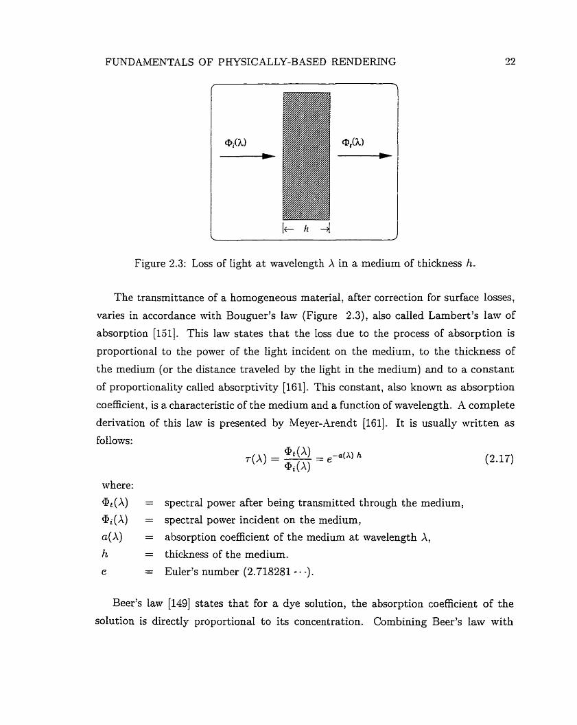
Figure 2.3: Loss of light a t wavelength A in a medium of thickness h.
The transmit tance of a homogeneous material, after correction for surface losses,
varies in accordance with Bouguer's Iaw (Figure 2.3), also called Lambert's law of
absorption [ltil]. This law states that the loss due to the process of absorption is
proportional to the power of the light incident on the medium, to the thickness of
the medium (or the distance traveled by the light in the medium) and to a constant
of proportionality called absorptivity [161]. This constant, also k n o m as absorption
coeficient, is a characteristic of the medium and a function of wavelength. -4 complete
derivation of this law is presented by Meyer-Arendt [161]. It is usually written as
follows:
where:
@,(A) = spectral power after being transmitted through the medium,
a i ( A ) = spectral power incident on the medium,
a(X) = absorption coefficient of the medium a t wavelength A,
h = thickness of the medium.
e = Euler's number (2.718281 . -) .
Beer's lam [149] states that for a dye solution, the absorption coefficient of the
solution is directly proportional to its concentration. Combining Beer's law with
FUNDAMENTALS OF PHYSICALLY-BASED RENDEEUNG 23
Bouguer's law [151] for samples of thickness h and concentration c results in the
following expression for the transmit t ance of a homogeneous mat erial:
where:
a(,\) = absorption coefficient of the medium at wavelength A,
c = concentration of the solution,
h = thickness of the medium,
e = Euler's number (2.718281 - - -).
Sometimes it is more convenient to specify the absorption of a medium by means
of the extinction coefficient [Mg], p, which is given by:
where:
a(A) = absorption coefficient of the medium a t wavelength A,
A, = wavelength of light in the medium.
2.4 Rendering Equation
Three major global illumination approaches have been used in rendering to simu-
late the light transfer mechanisms: ray tracing, radiosity and hybrid methods. Kajiya
[131] unified the discussion of global illumination methods with the rendering equa-
tion. This equation, also known as transport equation, can be expressed in terms of
radiances (Equation 2.20) on t h e basis of the ray law (the radiance is constant along
a line of sight between objects [198]), and the definition of the BDF. In a simplified
form it is given by:
total emitted propagated
Equation 2.20 states that the radiance of a point z on a surface, in a direction 3 and at wavelength X is given by the sum of the emitted radiance component, Le, and
FUNDAMENTALS OF PHYSICALLY-BASED RENDERING 24
the propagated radiance component. L,. Csually Le is known from the input data,
and the computation of L, constitutes the major cornputational
/ *
problem.
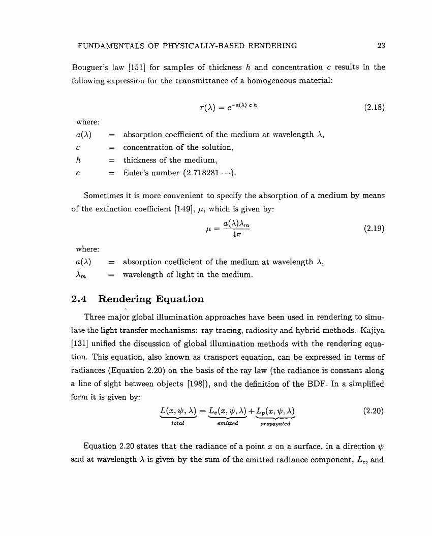
Figure 2.4: Geometry for computing L, as an integral over all the surfaces within the
environment.
The term L, can be written as an integral over al1 the surfaces within the environ-
ment (Figure 2.4) , resulting in the formulation presented in the follonring equation:
where:
f (x, , A) = BDF of the surface a t x,
L x , A) = spectral incident radiance at x and in a direction Si, Bi = angle behveen the surface normal a t x and the direction î/I,,
O, = angle between the surface normal a t xj aand the direction $iii,
d-4, = differential area surroundhg Xj7
V ( X , xj) - - visibility term.
The visibility t .em V(x . xj) used in the Equation 2.21 is one if a point xj of a
certain surface cari %eeY' a point x of another surface, and zero otherwise. This
equation is commonly used by deterministic rendering methods based on standard
numerical techniques [136]. In the context of global illumination t hese techniques are
used to solve the high dimensional integrals and large systems of eqiiations usually
associated mith the application of the radiosity method (Chapters 7 and 8).
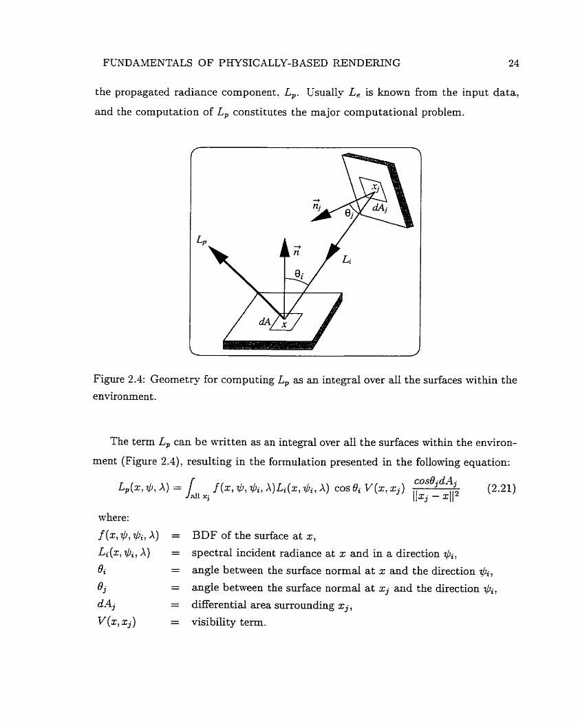
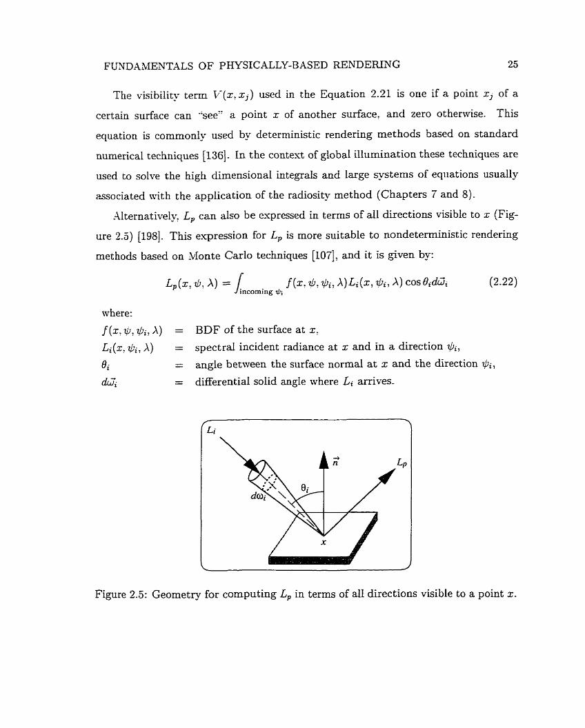
Alternati~ely~ L, can also be expressed in terms of al1 directions visible to x (Fig-
ure 2.3) [198]. This expression for L, is more suitable to nondeterministic rendering
methods based on Monte Car10 techniques [ l o i ] , and it is given by:
L, ( x : a9, A ) = / f ( x , Qi, X)Li(x, Ii,, A ) cos BidG (2.22) incoming iIt;
where:
f (xY +, $i, A ) = BDF of the surface at x:
Li(xY di , A) = spectral incident radiance at x and in a direction @i:
4 = angle between the surface normal a t x and the direction +i,
& = differential solid angle where Li arrives.
Figure 2.5: Geometry for computing L, in t e m s of al1 directions visible to a point x.
FUNDAMENTA4LS OF PHYSICALLY-BASED RENDERING 36
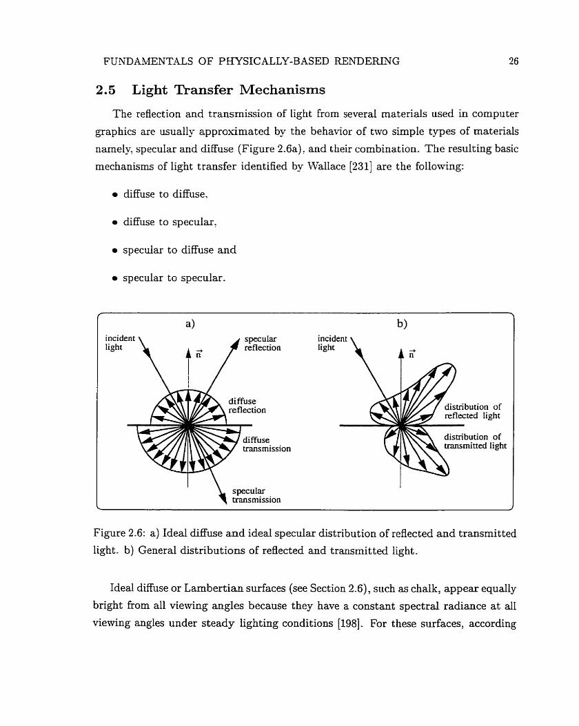
2.5 Light Transfer Mechanisms
The reflection and transmission of light fiom several materials used in computer
graphics are usually approsimated by the behavior of two simple types of materials
namely. specular and diffuse (Figure 2.6a), and their combination. The resulting basic
mechanisms of light transfer identified by Wallace [231] are the following:
diffuse to diffuse.
diffuse to specular,
specular to diffuse and
specular to specular-
r
distribution of
Figure 2.6: a) Ideal diffuse and ideal specular distribution of reflected and transmitted
light . b) General distributions of reflected and transmitted light .
Ideal diffuse or Lambertian surfaces (see Section 2.6), such as chalk, appear equally
bright from al1 viewing angles because they have a constant spectral radiance a t all
viewing angles under steady lighting conditions [198]. For these surfaces, according
FUNDAMENTALS OF PHYSICALLY-BASED RENDERTNG 27
to Lambert's cosine laiv of reflection [75]; the amount of radiant intensity seen by the
viewer is directly proportional only to the cosine of the angle of incidence of the light.
Specular surfaces: however. reflect light unequally in different directions. A perfect
specular surface; such as a rnirror, reflects Light only in the direction of retlection,
mhich corresponds to the viewer7s direction mirrored about the surface normal.
Act uai surfaces: honiever: present reflectance and transmit tance characteristics
which are quite varied and have a comples directional pattern (Figure 2.6b). Usu-
ally these surfaces are not adequately approximated by diffuse, specular, or cornbined
models [86]. Surfaces that approach closely the conditions of coherent (specular-like)
reflection are ordinarily said to be glossy, and those that approach closely the condi-
tions of incoherent (difise-like) reflection are said to be matte [El]. Surfaces that
allow some light to pass through are called transparent or translucent. The term
transparent is commonly used for surfaces that e-xhibit propagation characteristics
t hat can be bet ter approximated bÿ coherent transmission. The term translucent
is commonly used for surfaces whose propagation characteristics are better approxi-
mat ed by incoherent transmission.
The spectral energy distribution of the propagated light, measured in terms of
reflectance and transmittance, and the spatial distribution of that light, measured in
terms of BRDF and BTDF, mork together to establish the measurement of appearance
of an object [93]. This term is used to identify the family of measurements that are
necessary to characterize both the color and the surface finish of an object [122]. The
variations in the spectral energy distribution affect appearance characteristics such
as hue, lightness and saturation, which are described by Hunter and Harold [122] as
follows:
hue - attribute of color perception by means mhich an object is judged to be
red, yellonr, green, blue, purple and so forth,
lightness - perception by which white objects are distinguished from gray objects
and light from dark colored objects,
saturation - attribute of color perception that expresses the degree of departure
from the gray of the same lightness.
The changes in the spatial distribution affect appearance characteristics such as
gloss. reflection haze, transmission haze, luster and translucency. The reflection haze
corresponds to the scattering of reflected light in directions near that of specular
reflection by a specimen having a glossy surface [122]. The transmission haze corre-
sponds to the scattering of light within or at the surface of a nearly clear specimen,
responsible for cloudy appearance seen by transmission [1'22]. Finallu, the luster, or
contrast gloss. as described by Hunter and Harold [122], corresponds to the gloss
associated with contrasts of bright and less bright adjacent areas of the surface of an
object. Luster increases with increased ratio between light reflected in the specular
direction and that refiected in diffuse direction which are adjacent to the specular
direction.
Besides the interactions of direct light with individual objects, in order to perform
a general examination of light transfer mechanisms it is also necessary to account for
the indirect lighting. In this context, a notation suggested by Heckbert [Il71 can be
used to describe the direct and indirect light interactions with different objects in
an environment. He uses symbols to represent the various events experienced by a
photon. To avoid confusion with the radiometric terms used in this dissertation, we
will use boldface fonts to represent these symbols:
L - emission of a photon from a light source,
E - photon arriving a t the eye (intersection rvith the image plane),
V - photon interacting with a volume,
S - photon specularly reeected and/or transmitted,
D - photon diffusively reflected andior transmitted.
The sequence is written left to right over time, in such a way that L is the first
character and E is the last. Glassner [86] suggested the use of elements of the standard
cornputer-science regular expression symbology [Il91 to represent combined expres-
sions. As pointed out by Sillion and Puech [207], this notation approach can also be
used to characterize the shortcomings of the rendering methods [211]. For example,
FUNDAMENTALS OF PHYSICALLY-BASED RENDERING 29
distributed ray tracing [61] can in theory capture al1 possible paths followed by a
photon. which are represented by L(S ID)*E (where the verical bar 1 denotes a selec-
tion among members. and the asterisk superscript * represents O or more repetitions).
However. the diffiise information is rarely carried out explicitly by this method, due
to its high computational cost. Moreover, since this method is particularly suitable to
handle near-specular reflection and transmission. the term S can be replaced by the
glose t errn G. Thus. its characteristic expression is more appropriately represented
by L[D]G*E (where the square brackets indicate that the term D may be included
or not) [86].
In order to simulate various physical effects in the same scene, such as highlights
(view-dependent concentrations of light on a surface caused by non-diffuse refl ectors) , color-bleeding (diffuse reflection of light of one colored surface affecting the appearance
of another surface) and caustics (view-independent concentrations of Iight on a surface
caused by non-diffuse reflectors): one has to resort to multipass or hybrid algorithms
[JO, 116, 199, 2101.
The main idea behind these algorithms is that al1 the different paths of light trans-
fer that will be handled are determined beforehand, and each type of path is handled
only once [86]. For example, most of these algorithms start with a pass performed
by a radiosity method (Chapters 7 and 8) to determine the multiple diffuse inter-
reflections in the environment. Additional passes are performed by other rendering
methods to handle the other mechanisms of light transfer- Usually these passes are
performed by ray tracing methods such as visibility tracing [236], path tracing [131]
and photon tracing [174, 1751. The radiosity method takes into account the direct
light transfer paths from the light source, which are d s o accounted for by other ren-
dering methods. Then, it is necessas. to make sure that these direct paths are only
computed once. Usually their contribution is removed from the radiosity solution,
and computed again in one of the other passes, e.g. using photon tracing [198].
When applying the notation described earlier to these algorithms, usually each
tvpe of light transfer path or mechanism is represented by a specific characteristic
expression [86]. For example, Chen et al. [50] developed a hybrid algorithm in which
they considered four types of light transfer paths. The first type contains no diffuse
FUNDAMENTALS OF PHYSICALLY-BASED RENDERING 30
elements, and it is represented by LS*E. The second corresponds to a single diffuse
element with no specular surfaces between itself and the light: and it is represented by
LDS'E. The third is sirnilar to the previous, but with one or more specular elements
between the light and the d i f i se element, and it is represented by LSiDS*E (where
the plus-sign superscript + represents one or more repetitions). The fourth type
corresponds to a general case, nith two or more diffuse elements, and it is represented
by L(SID)*DS*DS*E.
2.6 Overview of Reflectance Models
The expression reflectance model is restrictive, since there are reflectance models
that handle transmittance as well. We will retain this term in this section for consis-
tency with graphics literature, explicitly mentioning the transrnittance components
when they become relevant. Moreover, since the reflectance models are in fact used
to determine the BRDF of the surfaces, we can often find the terrn BRDF model in
the literature. CVe suggest the term BDF model, which encapsulates the BTDF of
the surfaces as well.
Ueually reflectance models are divided into two families: empirical and theoretical
models [103, 189, 2331. The term empirical is somewhat misleading, since usually
these modeIs are not based on experimental data. In addition, they usually include
ad hoc terms in their formulation. Because of these aspects, we will henceforth refer
to these rnodels as ad hoc models. These models, although computationally simple,
are not physically plausible (Section 2.2) and lack the requirements needed for global
illumination calculations, namely energy conservation and reciprocity.
Theoretical models, on the other hand, are designed to attempt the fulfillment
of these requirements. These models may, in tum, be divided into two groups: an-
alytical and non-analytical models [189]. Analytical models provide an analytical
formulation to compute the BDF. Non-analytical models, on the other hand, use
an algorithmic process to compute the BDF for a selected number of incoming and
outgoing directions.
The sirnplest and oldest reflectance model is the Lambert model [86]. I t is named
after Lambert, who in 1760 introduced the cosine law of reflection (Section 2.5).
FUNDAMENTALS OF PHYSIC ALLY-BASED RENDERING 31
In computer graphics and computer vision Lambert's cosine law of reflection has
very often been assumed for diffuse-reflecting dielectric surfaces [239]. Recentl~; a
diffuse-reflective model for smooth dielectric surfaces was developed and used in ex-
perimental measurements by Wolff [239] to determine the range of applications of
Lambert's cosine law of reflection. These measurements showed that this law is a
good approximation (nithin approximately 3% accuracy) across illuminated smooth
dielectric ob jects svhen the angle of incidence and the viewing angle are simultane-
ously less than 50°- These measurements also showed that outside of this range large
deviations start to occur.
After the Lambert model, several reflectance models have been proposed by re-
searchers from different fields, such as physics, engineering, remote sensing (Chapter 3)
and computer graphics. In this section we will focus the discussion on reflectance
models aimed a t rendering applications? with a particular emphasis on works that are
considered milestones in this area. More comprehensive surveys on this topic can be
found in the papers by Schlick [188, 1891 and in the book by Glassner [86].
2.6.1 Ad Hoc and Transitiond Models
In 1973 Phong introduced a model [176], known as the Phong model, in which
an ad hoc exponentiated cosine is used to simulate specular highlights. Aftenvards,
Blinn [29] proposed a variant of the Phong model based on similar approximations,
but slightiy faster. \Vhile the Phong model does not have a physical basis, it can be
restricted to conserve energy. The BRDF resulting frorn these restrictions has been
used in global illumination calculations [123]. Lewis [146, 1471 has shown, however,
that this "Phong-like" BRDF does not satisfy the reciprocity condition.
In order to obtain a plausible BRDF, Lewis suggested modifications to the orig-
inal Phong model to make it reciprocal and constrained to conserve energy. These
changes originated a theoretical reflectance model Icnown as modified Phong model
(138, 1461. The plausible BRDF described by the modified Phong model has been
used to derive approximated PDFs for Monte Carlo integration through importance
sampling (see -4ppendix A). The scattering distributions derived fiom these PDFs,
in turn, have being used by nondeterministic physically-based rendering algorithms
[136] to simulate non-Lambertian phenomena [8, 7, 198: 199, 2031.
FUNDAMENTALS OF PHYSICALLY-BASED R E N D E W G 32
Some of the ad hoc models are called transitional models [103], since they began
a transition towards the energy equilibrium in rendering applications. The models
proposed by Kay and Greenberg [133] and Hall and Greenberg [104] are examples
of such models. The first model addresses attenuation of light passing through a
material while traveling between intersections. The second introduces an incoher-
ent transmission term to provide bet ter representation of light sources seen t hrough
objects.
2.6.2 Analytical Models
Torrance and Sparrom [222], working in the optical physics area, developed a
geometric refiectance model for specdar reflection based on a previous mork by Beck-
mann and Spizzichino [23]. Their model assumes that the surface is made of highly
reflective rnicroscopic facets distributed in v-grooves. The random distribution of the
facets allows the modeling of isotropic surfaces. -4 surface is qualified as isotropic
when the reflected light intensity at a given point is independent of the surface ori-
entation dong this normal a t this point. In other words, an isotropic surface has a
BRDF that is independent of rotation about the normal [233].
The normal vector to one of the two flat sides of a given groove is used, together
with the lighting direction and the viewing direction, to compute the fraction of
incoming light which is neither shadowed on the way in (shadowing), nor obscured
in the way out (masking). If the groves are randomly distributed over the surface,
shadowing and masking functions can be statistically estimated. Figure 2.7 shows
the effects of self-shadowing and self-masking by a rough surface. Therefore, using
these functions, the BRDF can be determined for a given distribution of dopes of the
facets.
The rnodel proposed by Torrance and Sparrow was applied to computer graphics
by Blim [29] and modified by Cook and Torrance [59] to take better account of colored
light. The Cook and Torrance model has been used to create very realistic pictures
of rnetallic and plastic objects. Besides having a physical basis, these models have in
cornmon the handling of isotropy. Several natural surfaces, such as forest canopies,
oceans, snow and sand, however, exhibit anisotropy. This means that if an element
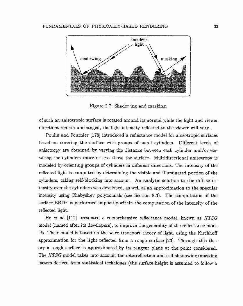
FUNDALMENTALS OF PHYSICALLY-BASED RENDERING
incident
Figure 2.7: ShadoNing and masking.
of such an anisotropic surface is rotated around its normal while the light and viewer
directions rernain unchanged; the light intensity reflected to the viewer mil1 Vary.
Poulin and Fournier [178] introduced a reflectance model for anisotropic surfaces
based on covering the surface with groups of small cylinders. Different levels of
anisotropy are obtained by varyïng the distance between each cylinder and/or ele-
vating the cylinders more or less above the surface. Multidirectional anisotropy is
modeled by orienting groups of cylinders in different directions. The intensity of the
reflected light is computed by determining the visible and illuminated portion of the
cylinders, taking self-blocking into account . An analytic solution to the diffuse in-
tensity over the cylinders was developed, as well as an approximation to the specular
intensity using Chebyshev polynomials (see Section 8.3). The coniputation of the
surface BRDF is performed implicitly within the computation of the intensity of the
reflect ed light . He et al. [112] presented a comprehensive reflectance modei, known as HTSG
model (narned after its developers), to improve the generality of the reflectance mod-
els. Their model is based on the wave transport theory of light, using the Kirchhoff
approximation for the light reflected from a rough surface [23]. Through this the-
ory a rough surface is approximated by its tangent plane at the point considered.
The HTSG model takes into account the interreflection and self-shadowîng/masking
factors derived from statistical techniques (the surface height is assumed to follow a
FUNDAMSNTALS O F PHYSICALLY-BASED mNDEFUNG 34
Gaussian distribution). They propose a BRDF consisting of three components: spec-
ular, directional-diffuse and uniform-diffuse. The first two components result from
the surface reflection process, due to specular reflection by the mean surface and
diffraction scat tering by the surface roughness respectively The t hird component is
attributed to multiple surface and/or subsurface reflections.
The HTSG model compares favorably with esperimental measurernents of re-
0ected radiation for metals. non-metals, and plastics, with smooth and rough surfaces.
The norrnalization mas, however: not adequately- treated in t his mode1 (2331. Furt her-
more, cornparisons between the reflectance model and absolute BRDF measurements
to demonstrate normalization empiricalIy were not made either. The authors claimed
that the data for the BRDF of rea1 surfaces is hard to corne bq; and they are sup-
ported in their da im by Shirley [198] and Ward [233] among other computer graphics
researchers.
-4s pointed out by Ward [233], a reflectance rnodel without symrnetry (reciprocity
of the BRDF described in Section 2.2) cannot be physical because the simulated
surface reflects light difFerently in one direction than the other. -41~0, without proper
normatization, a reflectance model does not yield a correct energy balance and, thus,
can no t produce phj-sically meaningful results. The models for anisotropic surfaces,
presented above, either fail to satisfy the one or the other of two physicai requirernents
or are sornewhat expensive to evaluate.
Waxd (2331 presented a mathematical model of anisotropic reflectance which was
extended from an isotropie Gaussian reflectance model similar to the model presented
by Cook and Torrance [59]. The BRDFs are computed through empirical formulas
that may incorporate Fresnel efTects. According to Ward, one of the advantages of
this model over more complex reflectance models, such as the HTSG model, is its sim-
plicity- It adapts to stochastic sampling techniques, which allows its implementation
through the Monte Carlo methods [107]. However, although this mode1 is accurate
for many surfaces, satisfying both reciprocity and normalization, there are still many
materials, such as translucent biological surfaces, that do not fit in the scope of the
model.
FUNDAMXNTALS OF PHYSICALLY-BASED RENDERING
2-6.3 Non-Analflical Models
The first model using an algorithmic approach was presented by Kajiya [130]. It is
also based on the wave transport theory of light, using the Kirchhoff appro-ximation
for reflection from a rough surface [23]. -4 numencal integration of the Kirchhoff
equation is done for each pair of directions in order to describe the reflection and
refraction of light from surfaces with anisotropic characteristics. This mode1 presents
some restrictions related to the self shadowing and multiple scattering, and it is
not considered computationally practical. It has the merit, however: of rederiving
the general formula for scattering from a rough surface in a form more suitable for
computer graphics.
Cabral et al. [44] proposed a model to generate anisotropic reflectance functions,
where the facets are created from a height field. The reflection of each facet is studied,
including the block factor for incident and reflected light, in order to compute the
surface BRDF. Cabral et al. c l a h that the anisotropy can be averaged out if desired
for isotropic surfaces. Sphericd harmonies series [86] are used to represent the BRDFs.
As with Kajiyak, this model is not considered to be computationally practical.
Westin et al. [235], extending the idea originally presented by Cabral e t al. [44],
proposed a general approach for approximating BDF for a large class of geometries.
While the two non-analytical models presented above can afford, a t best, to appros-
imate reciprocity. Westin et al. enforce the reciprocity by ensuring the symmetry of
the matris used to store the BDFs. The approach proposed by Westin et al. consists
of using a Monte Carlo ray tracing technique to simulate optical scattering. Moreover,
it provides the means of creating a milliscale BDF from microscale scattering events.
BDFs for complex surfaces can be simulated hierarchically by using the results of one
simulation in generating the BRDF for the next larger scale. This approach can be
applied to both isotropic and anisotropic materials such as brushed metals, velvet and
woven textiles. Oftentimes, however, the experimental data needed to describe this
hierarchical arrangement is not available, and the results may be difficult to validate
[109]. Although only three local scattering modes are described, namely specular
reflection, specular transmission and diffuse reflection, Westin et al. assert that their
approach allows the incorporation of other scattering modes as well.
FUNDAMENTALS OF PHYSICALLY-BASED RENDERING 36
Hanrahan and Krueger [IO91 proposed a similar6 model to simulate subsurface
scat tering and transmission from layered surfaces. known as the H- K multiple-layer
model [86]. This intuitive idea of a layered surface model has appeared several times
in physics [188], remote sensing (see Chapter 3) and cornputer graphics [188, 1981.
The algorithm to compute the BDF is based on the linear transport theory and
uses a Monte Carlo sampling scheme. The model esplicitly evaluates the reffection
and transmission of light at media boundaries, like in the ocean mode1 proposed by
Sishita et al. [171]. It assumes that the reflected radiance fiom a surface has two
components. One arises due to surface reflectance and the other due to subsurface
volume scattering- It also assumes that the transmitted radiance has two components.
One represents the amount of light transmitted through the layer without scattering
inside the layers, but accounting for absorption, and the other is due to scattering
in the volume. Similady. the BRDF and BTDF have also two components, and the
relative contributions of the surface and subsurface terms are modulated by Fresnel
coefficients. The physical plausibility of this approach was not demonstrated either
analytically or esperirnentaliy in spite of its physical basis.
The H-K multiple-layer model has the merit of addressing issues related to both
inorganic and organic rnaterials. However, its generality causes the overlook of impor-
tant specific characteristics and properties of organic materials, such as the absorption
of light by pigments. Moreover, the reflectance and transmittance are not computed
directly, but implicitly introduced into the model as the aibedo. In the context of
this model the albebo represents the ratio between the scattering cross section7 and
the sum of the scattering cross section and the absorption cross section. If the albedo
is close to zero, absorption is more likely to occur than scattering. In the testing
of the model on a plant leaf, Hanrahan and Krueger obtained the albedo values of
a leaf from an image acquired from a digital scanner. Although spectral ciirves of
reflectance and transmittance available in the literature could be used instead, for a
6We use the term similar in this context to refer to the fact that both algorithmic models, the
mode1 proposed by Westin et al. and the H-K rnodel, address subsurface phenomena and use Monte
Carlo techniques. 'In this context cross section may be interpreted as the probability per unit length of an inter-
action of a particular type [109].
FUNDAMENTALS O F PHYSICALLY-BASED RENDERING 37
large group of natural materials, specially- plant leaves, these spectral curves are only
available for a few illuminating and viewing angles.
Gondek et al. [93] have also proposed a mode1 which attempts to characterize the
reflectance functions of a material by modeling its subsurface microstructure. Their
model is mainly aimed a t paints. Gondek et al. define a substrate filled with small
pigment-particle microspheres. These particles are modeled as dielectric spectral
filters, and the attenuation of the transmitted light is poverned by Bouguer:s law
(Section 2.3). This mode1 serves to demonstrate some of the refiective properties that
real paints eshibit and simulate interference effects. More specifically: t his model is
used to predict thin film amplitude splitting interference. This phenornenon occurs
when a wave is divided through reflection and transmission? and later recombines
[93]. Gondek et al. state that, in order to turn their model into a true design tool,
comparisons must be perforrned against esperimental data taken from real surfaces
for which the surface and the subsurface geometries are known.
Schramm et al. [190] extended the model proposed by Gondek et al. to include
subsurface refraction and multilayer interference effects. They employed their mode1
to explore surface reflect ance prop erties of an iridescent hummingbird feat her and pa-
per. In the last case, measurements were taken to attempt to match actual reflectance
properties of the material. The results of these measurernents showed that the model
captured both the anisotropic refiectance functions caused by fiber orientation, and
the reflectance in the incident direction (backscatter or retroreflectanceg).
2.7 Summary
The rendering equation represents the kernel of global illumination met hods. In
order to solve this equation it is necessary to determine the reflection/transmission
behavior of the surfaces. This behavior is described by the BDF of the surfaces, which
is a combination of the BRDF and BTDF, or alternatively by the S P F (Section 2.2).
Severai models have been proposed to represent these macroscopic reflectance and
asdaces that present a high degree of retroreflection are sometimes said to have "negative gloss" [l28]. The reflectance of highway signs is an extreme example of retroreflection or "negative gloss" . Commercial surfaces such as paint, plastics, papers and textiles, no matter matte or glossy, show some degree of retroreflection.
FUNDAMENTALS OF PHYSICALLY-BASED RENDEFUiPJG 35
transmit t ance properties of surfaces. Theoretical models, in particular. are designed
to be physically plausible to enable p hysically- based rendering.
Despite the efforts in this area, the current modets still present limitations and, in
several cases. a low accuracy/cost ratio. -lot al1 t heoretical models fulfill the physical
requirements, namely normaiization and reciprocitl Very Eew are controlled by a
small number of simple and rneaningful parameters, and present a formulation Rith
a low computational cost. Another unsatisfactory point of the current models, as
mentioned by Schlick [189]; is the formulation of the BDF as a linear combination
with constant weights between the diffuse and specular components. For example: to
make the modified Phong Mode1 consenTe energy and be reciprocal at same time, the
BDF is formulated using this approach [146, 1471.
The justification for using this linear combination of weights is that, for several
rnaterials: the diffuse and the specular components corne from different physical phe-
nomena [189]. For example. a poiished surface, such as varnished wood, can be
thought of as a diffuse reflector covered with a thin dielectric coating. The light is
reflected from the coating in a coherent way (specular reflection) and reflected from
the substrate in an incoherent way (diffuse reflection). As noticed by Shirley [198],
such a linear combination with constant weights is incorrect because proportions of
diffuse and specular components are usually not constant, but rather a function of
the incident angle.
Finally, very few reflectance models used in rendering address issues specifically
associated with organic materïals. It is important to note, however, that researchers
from other fields have advanced further in this area. In the next chapter w-e present
reflectance models for plants, the organic materials within the scope of this disser-
tation, proposed by biologists and remote sensing researchers. Some of the concepts
and the biological data used in these models are relevant for this dissertation. We
believe that the incorporation of this information is essential to develop and validate
biologically and physicallÿ-based BDF models for rendering applications.
Interaction of Light with Plant Tissue
One of the major difficult ies in biologically and p hysically-based rendering is the
lack of available experimental data to be used as input or for testing parameters.
Appropriately Ward [233] pointed out that good science requires both theory and
data, and one is of little use mithout the other. Fortunately. in the case of plants,
there is a reasonable amount of information that c m be incorporated into rendering
applications.
Most of this information consists of experimental data for plant leaves, which are
the most important plant surface interacting with light [126]. .Mthough other plant
surfaces, such as stems and petals, present similar optical and structural character-
istics [80, 1341: the ways in which they absorb and propagate light and thus acquire
their color have not been fully investigated. Recently Biolley and Jay [26j presented
a work on the colorirnetry of roses. However, there is still a noticeable lack of under-
standing of the relationships between petal structure and pigment distribution [134].
For these reasons, we are going to focus on light interaction mith foliar tissues in this
châp ter.
A large amount of research has been performed in botany and remote sensing
regarding the reflectance and transmittance characteristics of leaves. Most of this
research considers the entire light spectrurn. However, since, for rendering purposes,
we are mainly interested in the visible region of the light spectrum, we are going to
stress the phenornena associated with this region in this chapter.
The remainder of this chapter is organized as follows:
Section 3.1 presents a structural description of foliar tissues.
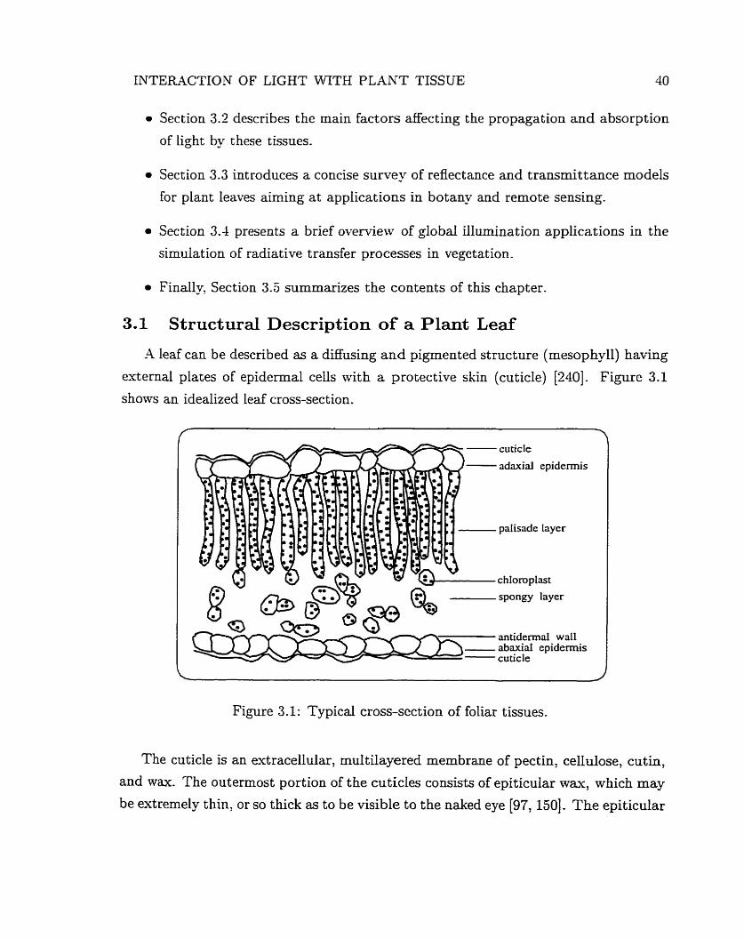
INTERACTION OF LIGHT WTTH PLANT TISSUE 40
Section 3.2 describes the main factors affecting the propagation and absorption
of light by these tissues.
0 Section 3.3 introduces a concise survey of reflectance and transmittance models
for plant leaves aiming a t applications in botany and remote sensing.
Section 3.1 presents a brief overview of global illumination applications in the
simulation of radiative transfer processes in vegetation.
Finaily, Section 3.3 summarizes the contents of this chapter.
3.1 Structural Description of a Plant Leaf
-4 Ieaf can be described as a diffusing and pigmented structure (mesophyll) having
extenial plates of epidermal cells with a protective skin (cuticle) [240]. Figure 3.1
shows an idealized leaf cross-sect ion.
cuticle
adaxial epidermis
palisade layer
chIoroptast
spongy layer
antidermai walI abaxial epidermis cuticle
.' Figure 3.1 : Typical cross-section of foliar tissues.
The cuticle is an extracellular, multilayered membrane of pectin, cellulose, cutin,
and wax. The outermost portion of the cuticles consists of epiticular wax, which may
be extremely thin, or so thick as to be visible to the naked eye [97,150]. T h e epiticular
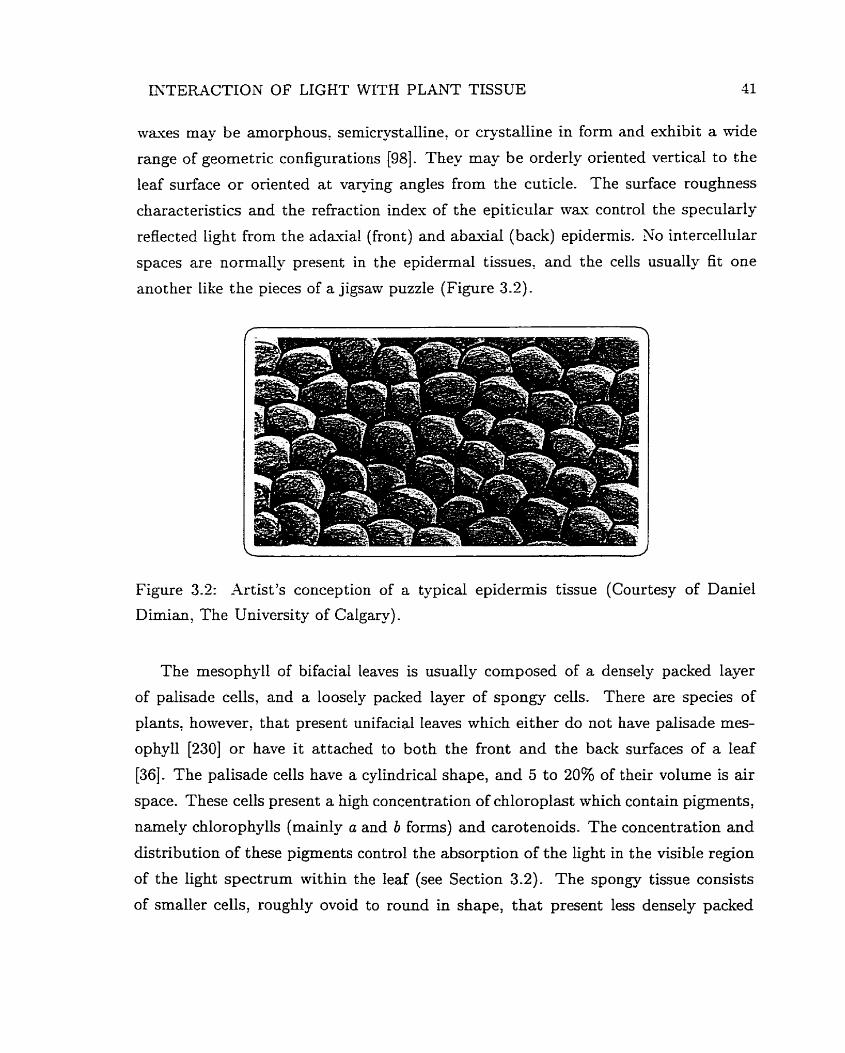
INTERACTION OF LIGHT WITH PLANT TISSUE 41
maves may be amorphous, semicrystalline: or crystalline in form and exhibit a wide
range of geornetric configurations [98]. They may be orderly onented vertical to the
leaf surface or onented a t v a ~ n g angles from the cuticle. The surface roughness
characteristics and the refraction index of the epiticular wax control the specularly
reffected light from the adaxial (front) and abaxial (back) epidermis. 30 intercellular
spaces are normal- present in the epidermal tissues: and the cells usually fit one
another Iike the pieces of a jigsanr puzzle (Figure 3.2).
Figure 3.2: Artist7s conception of a tipical epidermis tissue (Courtesy of Daniel
Dimian, The University of Calgary).
The mesophy11 of bifacial leaves is usually composed of a densely packed layer
of paiisade cells, and a loosely packed layer of spongy cells. There are species of
plants, however, t hat present unifacial leaves which either do not have palisade mes-
ophyll [230] or have it attached to Ooth the front and the back surfaces of a leaf
[36]. The palisade cells have a cylindrical shape, and 5 to 20% of their volume is air
space. These cells present a high concentration of chloroplast which contain pigments,
namely chlorophylls (rnainly a and b forms) and carotenoids. The concentration and
distribution of these pigments control the absorption of the light in the visible region
of the light spectrum within the Ieaf (see Section 3.2). The spongy tissue consists
of smaller cells, roughly ovoid to round in shape, that present less densely packed
INTERACTION OF LIGHT WITH PLANT TISSUE 42
chloroplasts, with 50 to 80% of their volume occupied by air space [240]. The spaces
between the mesophyll cells are also filled with air.
3.2 Factors Affecting the Propagation of Light
The reflection, transmission and absorption of light by leaves is affected by some
important leaf characteristics:
Interna1 Structure and Thickness
The intra-leaf scattering caused by refractive index differences between cel-
lular organelles, walls, hydrated cells, and adjacent intercellular air spaces is
cornpounded or amplified by the irregular shapes and organization of the cells
within the leaf [223]. -4s pointed out by Grant [97], differences in the reflectance
curves among species, as well as changes with maturation and senescence, have
also been attributed to differences in the leaf internal structure. These differ-
ences directly affect the thickness of the leaves. Experiments by wooley [240]
showed that, although the reflectance of a leaf is not strongly dependent on the
leaf t hickness, the transmit t ance is strongly affected by t his foliar characteristic.
Allen e t al. [3] assert that the differences in internal structure are substantial
between sun and shade Leaves of the same plant species. Clearly, even greater
differences can be expected between leaves from different species.
Pigments Composition, Concentration and Distribution
Experiments [223, 2401 showed that the reflectance of leaves is relatively low in
the visible portion of the light spectrum (400nm to 700nm), and that absorp-
tance dominates. Most of the absorption in this region is caused by pigments
presented in the leaf tissue. Pigments are materials that exhibit selective reflec-
tion and selective absorption [86]. The usual pigments found in leaves are the
chlorophylls and the caratenoids. -4s pointed out by Devlin and Baker [66], the
chlorophylls are by far the most important and abundant of these pigments, and
they are usually concentrated in the palisade mesophyll. There are several forms
of chlorophyll [228], and the dominant ones are chlorophylls a and b. Although
the relative pigment concentrations Vary within the species, most of the plants
INTERACTION OF LIGHT WITH PLANT TISSUE 43
contain two to three times more chlorophyll a than b [187]. These two forms
of chlorophyll present similar absorption spect ra (curve showing the absorption
coefficient of the material at various wavelengths): and sorne researchers com-
bine them into a single curve due to the high correlation between them [125].
The carotenoids are a group of pigments which. in higher plants. are usually
red. orange, yellow. or brown and are associated with chlorophyll in the chloro-
plasts [187]. Their yellow colors are evident in many autumn leaves from mhich
the chlorophyll has disappeared. Senescent leaves present also brown pigments
called tamis. However, to the best of our knowlodge, there is not yet a method
to determine the concentration of brown pigments [125].
Water Content
The concentration and distribution of water affects the absorption of light in
the infrared region, but have no significant effect on the absorption of light
in the visible region [223]. However, as ivater is Lost from a fully turgid leaf,
the reflectance increases. Different patterns in this increase are seen in different
types of leaves. Wooley [240] hypothesized that the reason might be the changes
in intercellular air spaces.
Surface Features
A small amount of incident light is initially reflected fiom the iipper cuticular
surface for angles of incidence srnaller than 45" [240]. Grant [97] states that
the presence of hairs in some species increases the reflectance, by presenting
numerous light scattering interfaces which decreased the amount of light en-
tering the leaf, thereby decreasing absorption. The reflectance curves of leaves
are also affected by their venation system [240]. It is likely that their increased
thickness and lower concentration of pigments affect the reflection and trans-
mission of light [98]. However, biological data regarding these characteristics of
the venation systems is scarce.
Grant et al. [97] describe leaves as having bot h specular and diffuse characteristics.
The specular (non-Lambertian) character of the leaf reflectance arises at the surface
of the leaf. For some viewing directions, the surface reflectance may be so large
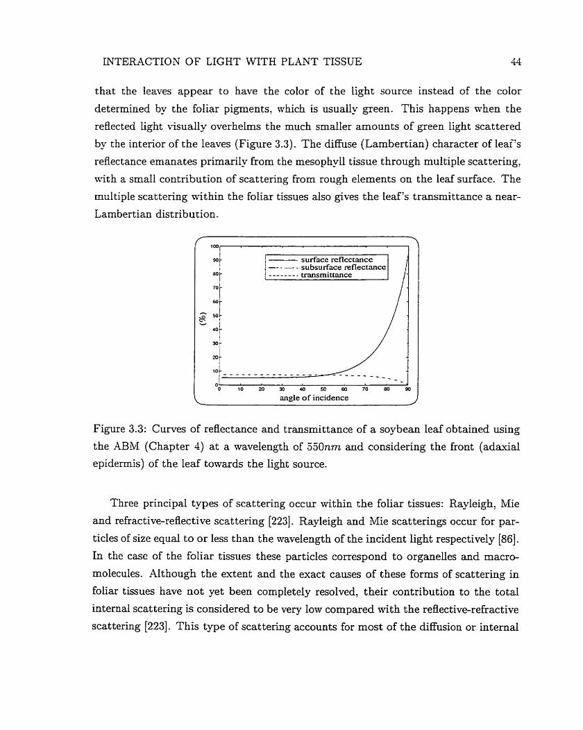
INTEMCTION OF LIGHT \VITH PLANT TISSUE 44
that the ieaves appear to have the color of the light source instead of the color
determined by the foliar pigments, which is usually green. This happens when the
reflected light cisually overhelms the much smaller amounts of green light scattered
by the interior of the leaves (Figure 3.3). The diffise (Lambertian) character of leaf's
reflectance emanates primarily from the mesophyll tissue through multiple scattering,
with a small contribution of scattering from rough elements on the leaf surface. The
multiple scat tering wit hin the foliar tissues aIso gives the Leaf's transmit t ance a near-
Lambertian distribution-
surface reflectance subsurface reflectance uansmittance
angle of incidence
Figure 3.3: Curves of reflectance and transmittance of a soybean leaf obtained using
the ABM (Chapter 4) at a wavelength of 550nm and considering the front (adaxial
epidermis) of the leaf towards the light source.
Three principal types of scattering occur within the foliar tissues: Rayleigh, Mie
and refractive-reflective scattering [223]. Rayleigh and Mie scatterings occur for par-
ticles of size equal to or less than the wavelength of the incident light respectively [86].
In the case of the foliar tissues these particles correspond to organelles and macro-
molecules. -4lthough the extent and the exact causes of these forms of scattering in
foliar tissues have not yet been completely resolved, their contribution to the total
interna1 scattering is considered to be very Iow compared with the reflective-refractive
scattering [223]. This type of scattering accounts for most of the difision or internai
INTERACTION OF LLGHT WITK PLANT TISSUE 45
scattering, and it is mainl- caused by the arrangement of tissues. and the refractive
indes differences, which? for the most part. are associated wïth air-ce11 wall interfaces
regarding cells whose dimensions are quite large compared with the wavelength of
light such as the palisade and spongy cells.
In species having bifacial leaves the adaxial epidermis is attached to the mesophyll
over most of its inner surface (Figure 3.1), so that once light has passed the outer
epidermal surface. it can easily pass into the center of the leaf. The light entering
or leaving the abaxial surface of a leaf must, however: p a s through two serniplanar
interfaces, namely the air-abaxial epidermis and the air-antidermal wall interfaces
(Figure 3.1). Thus light from a source on the back side of a leaf can penetrate the
back epidermis and be reflected back by the inside surface of the epidermis without
encountering the mesophyll. It is largely because of this aspect that the back of the
leaves is often pale. Moreover, these structural differences make the abaxial surface
of a leaf a greater barrier to the escape of the oblique light than the adaxial surface.
These factors explain why leaves that differ markedly in the structure of their two
sides show corresponding differences in their reflectance and transmittance curves
[24O].
Experiments performed by Wooley on maize leaves [240] showed that these leaves
reflect Iight more diffusively in a pIane perpendicular to the veins than in a plane
parallel to the veins. This aspect suggests that the anisotropy of pIant leaves is
associated Nith the venation systems. -4s described by Esau [72], a leaf may have
a single vein or two or more. Single-veined leaves are found among conifers', while
multiveined leaves are common in higher ferns2 and angiosperms3. Although the
major venation system of these species can be divided in two main types of patterns,
'Conifers correspond to one of the major groups of gyrnnosperms (vascuiar and flowerless plants
characterized by the presence of seeds). They typicaily bear cones and needle-like Ieaves, e.g. pine
and redwood [24]- 'Ferns form the most wideIy known group of pteridophytes (vascular and flowerless plants which
do not produce seeds)- They present feathery fronds formed by large leaves, u s u d y deeply parted
or divided, e.g. wood fem [24]- 3Angiosperms, or fiowering plants, dominate large areas of the land surface and represent the
climax of vascular plant evolution. They are very diversified in their form and range in size fkom
few milIimiters in diameter (aquatic Lemna) to over 90 meterç in height (Eucalyptus) [36].
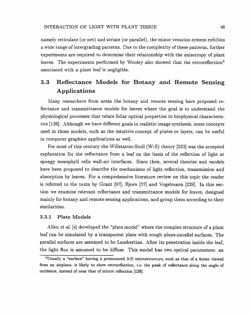
INTERACTION OF LIGHT WITH PLANT TISSUE 46
namely reticulate (or net) and striate (or parallel) the minor venation system exhibits
a wide range of intergrading patterns. Due to the cornplesïty of these patterns, further
experiments are required to determine their relationship svith the anisotropy of plant
leaves. The esperiments performed by Wooley aiso shonred that the retroreflection'
associated with a plant leaf is negligible.
3.3 Reflectance Models for Botany and Remote Sensing
Applications
Many researchers from areas like botany and remote sensing have proposed re-
flectance and transmittance modeIs for leaves where the goal is to understand the
physiological processes t hat relate foliar optical propert ies to biophysical characteris-
tics [126]. Although we have different goals in realistic image synthesis, some concepts
used in those models, such as the intuitive concept of plates or layers, can be useful
in cornputer graphics applications as well.
For most of this century the Willstatter-Stol1 (W-S) theory [223] was the accepted
exphnation for the reflectance from a leaf on the basis of the reflection of light a t
spongy mesophyll cells wall-air interfaces. Since then, several theories and models
have been proposed to describe the mechanisms of light reflection, transmission and
absorption by leaves. For a comprehensive literature review on this topic the reader
is referred to the texts by Grant [97], Bjorn [27] and Vogelmann [229]. In this sec-
tion we examine relevant reflectance and transmittance models for leaves, designed
mainly for botany and remote sensing applications, and group them according to their
similarit ies.
3.3.1 Plate Models
Allen et al. [4] developed the "plate model" where the complex structure of a plant
leaf can be simulated by a transparent plate with rough plane-parallel surfaces. The
parallel surfaces are assumed to be Lambertian. After its penetration inside the leaf,
the light flux is assumed to be diffuse. This model has two optical parameters: an
4Usually a "surface" having a pronounced 3-D microstructure, such as that of a forest viewed
from an airphne, is likely to show retroreflection, Le. the peak of refiectance dong the angIe of
incidence, instead of near that of mirror reflection [128].
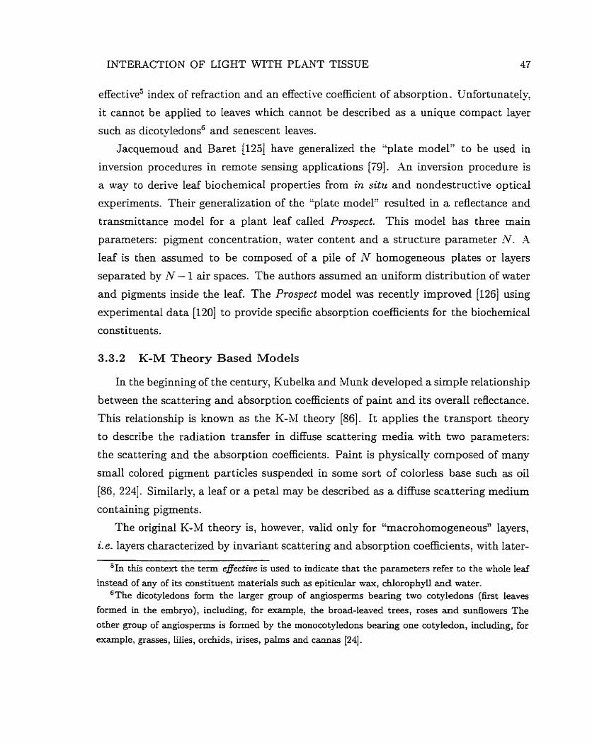
INTERACTION OF LIGHT WITH PLANT TISSUE 47
effective5 index of refraction and an effective coefficient of absorption. Unfortunatel-
it cannot be applied to leaves which cannot be described as a unique compact layer
such as dicotyledons6 and senescent leaves.
Jacquemoud and Baret [Es] have geoeraiized the "plate model" to be used in
inversion procedures in remote sensing applications [Tg]. An inversion procedure is
a way to derive leaf biochemical properties from in situ and nondestructive optical
expe~ments. Their generalization of the "plate model" resulted in a reflectance and
transmittance mode1 for a plant leaf called Prospect. This mode1 has three main
parameters: pigment concentration, water content and a structure parameter N. -4
Ieaf is then assumed to be composed of a pile of iV homogeneous plates or layers
separated by N - 1 air spaces. The authors assumed an unifonn distribution of water
and pigments inside the leaf. The Prospect model was recently improved [126] using
experimental data [120] to provide specific absorption coefficients for the biochemical
constituents.
3.3.2 K-M Theory Based Models
In the beginning of the c e n t u q Kubelka and Munk developed a simple relationship
between the scattering and absorption coefficients of paint and its overall reflectance.
This relationship is known as the K-;LI theory [86]. It applies the transport theory
to describe the radiation transfer in diffuse scattering media with two parameters:
the scattering and the absorption coefficients. Paint is physically composed of many
srnall colored pigment particles suspended in some sort of colorless base such as oil
[86, 2241. Similarly, a Leaf or a petal may be described as a diffuse scattering medium
containing pigments.
The original K-M theory is, however, valid only for "macrohomogeneous" layers,
i-e. layers characterized by invariant scattering and absorption coefficients, with later-
% tthis context the term effective is used to indicate that the parameters refer to the whole leaf
instead of any of its constituent materials such as epiticular m-aq chlorophyU and water. 'The dicotyledons form the larger group of angiosperms bearing two cotyledons (first leaves
formed in the embryo), including, for example, the broad-leaved trees, roses and sunîîowers The other group of angiosperms is formed by the monocotyIedons bearing one cotyledon, including, for
example, grasses, Hies, orchids, irises, palms and cannas [24].
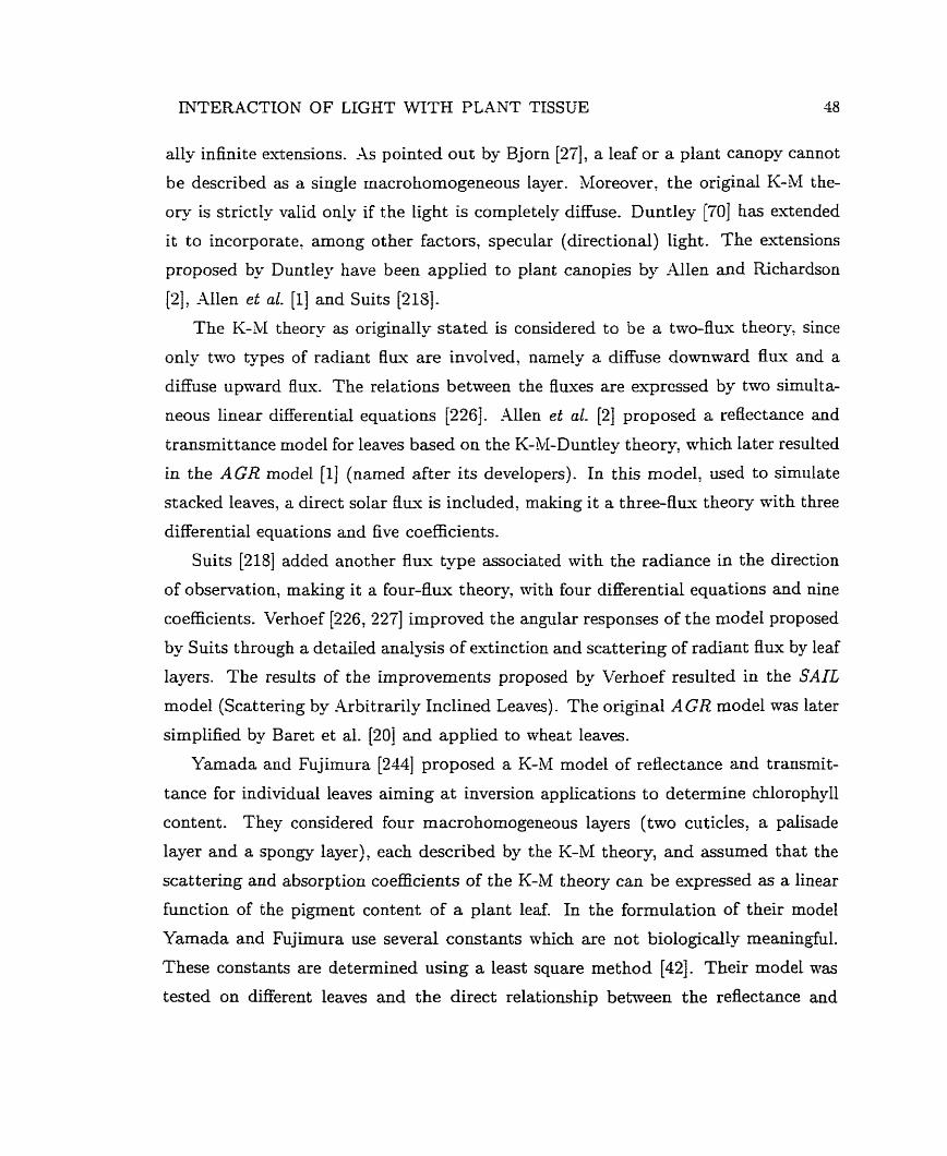
INTERACTION O F LIGHT WITH PLANT TISSUE 48
ally infinite extensions. -1s pointed out by Bjorn [Z], a leaf or a plant canopy cannot
be described as a single macrohomogeneous layer. Moreover. the original K-M the-
ory is strictly valid only if the light is completely diffuse. Duntley [70] has extended
it to incorporate, among ot her factors, specular (directional) light . The extensions
proposed by Duntley have been applied to plant canopies by Allen and Richardson
[2], Allen et al. [Il and Suits [218].
The K-hl theory as originally stated is considered to be a two-flux theov: since
only tnro types of radiant flux are involved, namely a diffuse downward flu'r and a
diffuse upward flux. The relations between the f lues are expressed by two simulta-
neous linear differential equations [226]. Allen et al. [2] proposed a reflectance and
transmittance model for leaves based on the K-Id-Duntley theos; which later resulted
in the AGR rnodel [Il (narned after its developers). In this model, used to simulate
stacked leaves, a direct solar flux is included, making it a three-flux theory with three
differential equations and five coefficients.
Suits [218] added another flux type associated with the radiance in the direction
of observation, rnaking it a four-flux theory, with four differential equations and nine
coefficients. Verhoef [226, 2271 improved the angular responses of the rnodel proposed
by Suits through a detailed analysis of extinction and scattering of radiant flux by leaf
layers. The results of the irnprovernents proposed by Verhoef resulted in the SAIL
model (Scattering by Arbitrarily Inclined Leaves). The original AGR rnodel was later
simplified by Baret et al. [20] and applied to wheat leaves.
Yamada and Fujimura [244] proposed a K-M model of reflectance and transmit-
tance for individual leaves aiming a t inversion applications to determine chlorophyll
content. They considered four macrohomogeneous layers (two cuticles, a palisade
layer and a spongy layer), each described by the K-M theory, and assumed that the
scattering and absorption coefficients of the K-M theory can be eAxpressed as a linear
function of the pigment content of a plant leaf. In the formulation of their model
Yamada and Fujimura use several constants which are not biologicalb meaningful.
Shese constants are deterrnined using a least square method [42]. Their model was
tested on different leaves and the direct relationship between the reflectance and
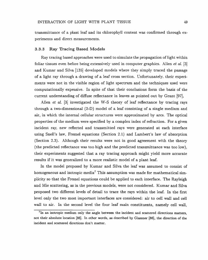
INTEMCTION OF LIGHT WITH PLANT TISSUE 49
transmittance of a plant leaf and its chlorophyll content svas confirmed through ex-
periments and direct measurements.
3.3.3 Ray Tracing Based Models
Ray tracing based approaches svere used to simulate the propagation of light within
foliar tissues even before being estensively used in computer graphies. Allen et al. [3]
and Kumar and Silva [135] developed models where they simply traced the passage
of a light ray through a drasving of a leaf cross section. Unfortunatel?: their experi-
ments svere not in the visible region of light spectrum and the techniques used were
computationally expensive. In spite of thac their conclusions form the basis of the
current understanding of diffuse reflectance in leaves as pointed out by Grant [97],
Allen et al. [3] investigated the W-S theory of leaf reflectance by tracing rays
through a two-dimensional (243) model of a leaf consisting of a single medium and
air, in which the interna1 ceilular structures were approximated by arcs. The optical
properties of the medium were speczed by a complex index of refraction. For a given
incident ray, nem reflected and transmitted rays were generated a t each interface
using Snell's lasv, Fresnel equations (Section 2.1) and Lambert's law of absorption
(Section 2.3). Although their results were not in good agreement svith the theory
(the predicted reflectance svas too high and the predicted transmittance was too low),
their experiments suggested that a ray tracing approach might yield more accurate
results if it svas generalized to a more realistic model of a plant leaf.
In the mode1 proposed by Kumar and Silva the leaf was assumed to consist of
homogeneous and isotropic media7 This assumption \vas made for mathematical sim-
plicity so that the Fresnel equations could be applied to each interface. The Rayleigh
and Mie scattering, as in the previous models, were not considered- Kumar and Silva
proposed two different levels of detail to trace the rays within the leaf. In the first
level only the two most important interfaces are considered: air to cell wall and ce11
wall to air. In the second level the four leaf main constituents, namely ce11 wall,
71n an isotropic medium only the angle between the incident and scattered directions matters,
nct their absolute Iocation [86]. In other words, as described by Glaçsner [86], the direction of the
incident and scattered directions don't matter.
INTERACTION O F LIGHT WITH PLANT TISSUE 50
chloroplasts: ce11 Sap and air. give raise to the folloming eight optical interfaces in the
leaf. all of which were considered in the ray tracing:
air to cell.
ce11 Sap to ce11 wall,
chloroplasts to ce11 wall,
cell Sap to chloroplasts,
ce11 wall to chloroplasts:
ce11 wall to ce11 Sap and
ce11 wall to air.
Their experiments showed that considering only ce11 wall to air and air to ce11
wall interfaces is likely to give less diffuse reflectance and transmittance than that
given by considering al1 the eight interfaces. Kumar and Silva also claimed that their
model can be used to simulate the optical phenornena in the visible region of the light
spectrum t hrough the use of appropriate indexes of refraction of the leaf constituents
in the visible region.
Recently Govaerts et al. [96] proposed a Monte Car10 ray tracing based model
to simulate the propagation of light in a typical dicotyledon leaf. In their simulation
approach the three-dimensional (3-D) interna1 cellular structure of various leaf tissues
is explicitly geometrically modeled. -4 typical foliar ce11 is defined by Govaerts et al. as
a set of concentric objects filled with three different media, namely ce11 wall material,
water and chlorophyll, and the different shapes of these cells are approximated by
primitive objects such as spheres, ellipsoids and cylinders. Although the modeling
of individual cells may improve the accuracy of the simulations, the complexiS of
the resulting (3-D) geometrical model is likely to place a substantial demand on
computational resources to trace the ray paths.
INTERACTION OF LIGHT WITH PLANT TISSUE 51
In their model, each ce11 constituent is characterized by an index of refraction
and an absorption coefficient. The interaction of light with various ce11 constituents
is also simulated using the Fresnel Equations (Section 2.1). The absorption testing
assumes a homogeneous distribution of pigments, and it is performed probabilistically,
using a n expression based on Beer's law (Section 2.3), and considering the incident
rays perpendicular to the interfaces. Although the results presented by the model
proposed by Govaerts et al. seemed to qualitatively approximate the spectral curves
of a plant leaf. direct cornparisons with Cumes obtained experimentally would be
needed to determine the quantitative accuracÿ of their results.
3.3.4 Radiat ive Transfer Theory Based Models
Tucker and Garret [223] proposed a stochastic leaf radiation model based upon
leaf structure: pigment composition and concentration of water content. The radia-
tive interactions within a leaf are considered as a random walk process [107], using
the Markov chainS approach. Their stochastic model compartmentalizes a leaf to rep-
resent the radiation states, cell parts, and interna1 scattering. The radiation states,
namely reflected, absorbed, and transmit ted, are represented by siu compartments:
solar input;
reflection from cuticle;
absorption in the palisade celIs;
diffuse reflected radiation;
absorption in the spongy cells;
diffuse transmit ted radiation.
Although the model predictions for leaf spectral absorption, reflection, and trans-
mission closely agree with measured values for the non-visible region of the light
*A sequence of raodom variables, xo , xi, xz , ..., generated such that at each time t > 0, the next
state xt+l is sampled fiom a distribution P(xttl 1 xt), which depends only on the curent state of
the chain, xt, is c d e d a Markov chain [85].
INTEMCTION OF LIGHT W T H PLANT TISSUE 52
spectrum, the simulation results did not account for the high degree of absorption
mhich occurs in the visible region. Yevertheless? t his model provides a technically
sound approach for simulating light interactions with plant leaves. Tucker and Gar-
ret daim that the success in their modeling approach depends upon the calculation
and justification of accurate probabilities to represent the flows between and within
states.
kla et al. [150] also used the radiative transfer t h e o ~ combined with wave optics
to develop a model in which a leaf is modeled as a slab of water with a irregular
surface and containing randomly distributed scatterers. They assume that the surface
roughness is of relatively great size compared with the incident wavelength and it
undulates on a large scale. This assumption allowed them to apply the Kirchhoff
rough surface scattering theory 1231 to describe the leaf surface reflectance. Ma et
al. assumed that the scatterers inside the leaf are spherical to enable them to apply
a scat tering function derived from the Mie scat tering t heory. The optical scat tering
within a leaf was simulated by combining the multiple scattering with the Kirchhoff
rough surface theory.
Ma et al. solved the radiative transfer equations with Stokes vectors and boundary
conditions [45] numerically using Fourier expansion, a discrete-ordinate technique and
an eigenvalue-eigenvector method [124, 1521. Instead of providing spectral curves of
refl ectance and transmittance, the model proposed by Ma et al. determines optical
parameters for different plant leaves, such as optical thicknessg, surface roughness
and refractive indexes. These parameters can, in turn, be incorporated into standard
reflectance and transmittance models. Ma et al. also considered the depolarization of
the polarized incident beam used in their experiments. Although Ma et al. claimed
that they have modeled a leaf as a slab of water because the high water content of
fresh leaves, as mentioned earlier, the role of the absorption pigments in the optical
phenornena occurring within a leaf cannot be overlooked.
' ~ h e optical thickness, as presented by Ma et al. is given by the product of the distance dong
z axis (thickness) by the particle number density and the total scattering cross section per particle.
INTEFUCTION O F LIGHT W T H PLANT TISSUE
3.4 Global Illumination Applications in Vegetation
In the previous sections we addressed issues mainly related t O the interaction
of light wïth individual leaves. In this section m-e provide an overview of global
illumination applications for radiat ive t ransfer in regions of vegetation such as forest
canopies or crops. Radiation transport in plant canopies have been extensively st udied
for interpreting remote sensing data [l63], such as satellite images used t o survey land
use and resources, and for predicting vegetation productivity, lit ter decomposition
processes and nutrient cycles within an ecosystem (791.
From the point of viem of a satellite regions of vegetation are "surfaces" n i th a
characteristic BDF that detennines their appearance under various observation con-
ditions [57]. In order to determine the BDF of a region of vegetation, such as a forest
canopy, a model of this vegetation canopy can be constructed and evaluated through
cornputer simulations [88]. Simplified models used in these applications usually treat
a canopy as a system of homogeneous volume elements with a certain density. A
model of radiative transfer is then used to compute the radiation transport between
these volumes [jï, 881.
For heterogeneous environments the radiative transfer processes are simulated us-
ing Monte Carlo methods [181, 1821, which were introduced to plant canopy radiative
transfer studies by Tanaka [220]. The application of these methods is done through
the simulation of solar radiation transfer processes as an aperiodic Markov chain of
collisions between photons and foliar tissues. Ross and Marshak [182] provide a de-
tailed review of works in this area and their contributions to the development of a
plant canopy radiative transfer theory.
As mentioned by Ross and Marshak, besides its suitability to the simulation of
radiative transfer in 3-D inhomogeneous canopies, the use of Monte Carlo methods
involves additional advantages. I t allows the consideration of the detailed architecture
of individual plants, the shape and the area of the Ieaves, the penumbral effects by
penetration of direct solar radiation. Moreover, it also permits the calculation of
the statistical characteristics of fluxes and intensities. However, t o obtain results
of acceptable accuracy a great number of trials is needed, which may increase the
computational costs considerably.
INTERACTION OF LIGHT WITH PLANT TISSUE 54
Recently. remote sensing researchers and plant biologists started to resort to global
illumination approaches developed or improved by the computer graphics community
as alternative solutions to simulate radiation transport in plant canopies. Among
these approaches is the radiosity method (Chapters 7 and 8). Gerst and Borel [84]
and Borel et al. [35] have applied this method to simulate radiative transfer in canopies
with several thousand of leaves, and Goel et al. [S9] have applied it to simulations of
radiative transfer in cornfields-
As mectioned by Borel et al. [35] , the strength of the radiosity method for these
applications is the capability of describing quantitatively and physicaliy correctly
the interactions of radiation with ma- surfaces that may be arranged in a complex
structure such as a plant canopy. Among the drawbacks of this method one can high-
light the difficulties to handle non-Lambertian phenomena. Moreover, t his met hod
may demand large computational resources for certain applications, e-g. scenes with
millions of primitives. Fortunately: one can take advantage of techniques used in
computer graphics, such as the clustering of objects hierarchically into volumes [206]
and the application of hierarchical radiosity methods [56, 110, 111, 1961, t o minimize
the computational costs.
Methods combining different global illumination techniques have also been used to
perform radiative transfer simulations in plant canopies. Govaerts [95] used a Monte
Carlo ray tracing algorithm; and Chelle [47] proposed an hybrid approach in which
the radiosity method is used for elements of a region of vegetation close to a point of
interest and the SAIL mode1 (Section 3.32) is used for elements distants from this
point of interest. This approach \vas called nested radiosity for plant canopies [48].
Recently, Mech [158] used a radiosity via ray tracing algorithm [201], also based on
Monte Carlo methods, to compute the arnount of light reaching plant organs in a
given environment - The Monte Carlo ray tracing based algorithms can be applied to complex envi-
ronments and are easy to implement. A large number of rays, however, is usually
required in order to converge to an accurate solution. Moreover, if there are lighting
and reflectance changes in the environment the entire process of "shooting" rays to
determine the energy balance in the environment must be repeated. For this case,
INTEIWCTION OF LIGHT WITH PLANT TISSUE 55
the application of the standard radiosity may be more appropriate. We exanine this
issue in more detail in Chapter 8.
Recently May et al. [155] proposed a plane-parallel radiance transport approach
for global illumination in vegetation. In this approach the radiance transport problem
is reduced to one dimension (1-D) by assuming that the radiance depends angularly
on light flow directly on the unit sphere: but positionally only on zy the height above
the ground. The resulting partial differential equations are solved by the Runge-Kutta
method [QI. Max et al. claim that it is a good approximation for dense vegetation,
although it is not suitable for isolated trees.
One of the problems of applying global illumination methods for radiative transfer
in regions of vegetation, such as forest canopies and crops, is the scarce amount of an-
alytical or experirnental results to evaluate these methods under these circurnstances.
Usually the results regarding a proposed approach are compared with the results
provided by a different approach based on similar assumptions. If they present a
good agreement, the accuracy of the proposed approach is considered satisfactory, al-
though they may be both far from the real solution. Nevertheless, since most of these
approaches consider the volume elements or leaves as presenting only Lambertian
charact eristics, the incorporation of physically and biologically-based models includ-
ing non-Lambertian effects and absorption for these elements is likely to increase the
overall accuracy of these approaches.
The efficiency of the radiative transfer methods for plant canopies is directly asso-
ciated with the efficiency of the global illumination algorithms used in these applica-
tions. Improvements on these algorithms would reduce the computational overhead
of these applications. For instance, computing the radiosity at al1 positions necessary
to account for all sources of radiation in a vegetation canopy usually involves the
iterative solution of a large Linear system. Clearly the investigation of faster solutions
for these systems (Chapters 7 and 8) would improve the efficiency of the radiative
transfer approaches for plant canopies, not only for remote sensing purposes 1481, but
also for rendering purposes.
INTERACTION OF LIGHT WITH PLANT TISSUE 56
3.5 Summary
In this chapter me have surnmarized the main aspects of light interaction with
plants. In order to simulate the mechanisms of photon transport within the foliar
tissues- it is necessary to account for the biological and structural characteristics of
these tissues and their components. Factors like the presence of pigments and the
interna1 distribution of the tissues have a significant impact on how leaves propagate
and absorb light.
Several rnodels have been proposed by remote sensing researchers and plant biol-
ogists to describe the reflectance and transmit tance characteristics of leaves- These
models present different levels of complexity and propose different techniques to de-
scribe and sirnulate light propagation within the foliar tissues. Although these models
have not been designed for rendering applications, they provide valuable information
that can be incorporated in the design of models airning at these applications.
A substantial amount of research has also been done to describe and simulate
the radiative transfer processes in vegetation. Although most of the research on this
topic has been restricted to remote sensing applications, the fundamental aspects
involved in these processes are also relevant for the rendering of natural scenes. Xot
surprisingly global illumination methods used in rendering applications have been
incorporated by remote sensing researchers in their studies of radiative transfer in
plant canopies.
The local and global levels of light interaction with plants, namely the reflectance
models for individual leaves and the radiative transfer processes for canopies, are
directly connected. New developments or improvements on either level, or in both,
will have a direct influence on the accuracy and eEciency of the rendering methods
for natural scenes. In the next chapters we intend to address these issues and present
our contributions.
CHAPTER 4
The Algorithmic BDF Mode1 for Plant Tissue
Although many physicaliy plausible BDF models have been proposed in the computer
graphics literature (Section 2.2). there is still a lack of models aimed a t biological ma-
terials. In this chap ter we address this issue through the presentation of an algorithmic
BDF model (ABM) that accounts for biological factors that affect light propagation
and absorption in plant tissues. The model is oriented to leaves, since, as mentioned
earlier, they are the most important plant surface interacting with light. However,
it c m be esitended to other plant surfaces like petals and stems since they present
similar optical and structural characteristics [80, 1341.
Many BDF models used in computer graphics rely on values of reflectance and
transmittance either set by the user or obtained from the literature. Although spec-
tral reflectance and transmittance curves are available for leaves [81, 98, 1001, they
are restricted to a narrow range of illuminating and viewing angles. Thus, it be-
cornes necessary to design a BDF rnodel for plant tissue in which the reflectances and
transmittances are calculated by the model itself.
An exact geometrical model of a plant tissue would rnodel individual cells and
their interior details explicitly. The geometrical model used by Govaerts et al. [96]
(Section 3.3.3) is an example of such an approach. The drawbacks of using such a
detailed geometrical rnodel in the simulation of light interaction witith foliar tissues
are the large number of parameters involved, which rnakes control difficult, and its
significant implementation overhead. Our strategy is to use a higher level of abstrac-
tion, which allows Our BDF rnodel to be controlled by a small number of biologically
meaninghil parameters and enables its easy incorporation into global illumination
frameworks.
THE ALGORITHMIC BDF MODEL FOR PLANT TISSUE 58
The implementation of the ABM is based on an algorithmic process using Monte
Carlo methods [107. 1321. Thus. the BDF of a foliar tissue can be calculated and
used on the fly during the rendering process, or computed off-line and stored to
be reconstructed during rendering (Chapter 5 ) or used for validation purposes. We
compare the results obtained using the ABM wit h available esperimental data.
The remainder of this chapter is organized as follows:
Section 4.1 introduces the algorithmic BDF model.
Section 4.2 presents the algorithms used to simulate the scattering profile of the
foliar tissues.
Section 4.3 describes the algorithms used to account for the absorption within
t hese tissues.
Section 4.4 presents an overview of the model's implementation and a summary
of its parameters.
Section 4.8 presents the procedures and parameters used to test the ABM,
focusing on the cornputer simulation of measurement devices.
Section 4.6 discusses the results and performance issues.
The chapter closes with a summary of the main characteristics of the ABM.
4.1 Outline of the Algorithmic BDF Mode1
In the ABM light propagation is described in terms of ray optics. The foliar
tissues are assumed to be isotropic due to the lack of experimental data on factors
affecting the anisotropy of plant leaves (Chapter 3). Moreover. the refractive-reflective
scattering is assumed to be the dominant form of scattering within the foliar tissues,
mhich is consistent with the literature regarding this topic (Chapter 3).
Instead of geometrically modeling many cells individually, the propagation of light
Nithin these tissues is simulated as a stochastic process whose states are associated
with the air-ce11 wall interfaces represented in Figure 4.1. Once a ray hits a leaf at
interface 1 or interface 4 (state 1 or state 4), it can be reflected back to the environment
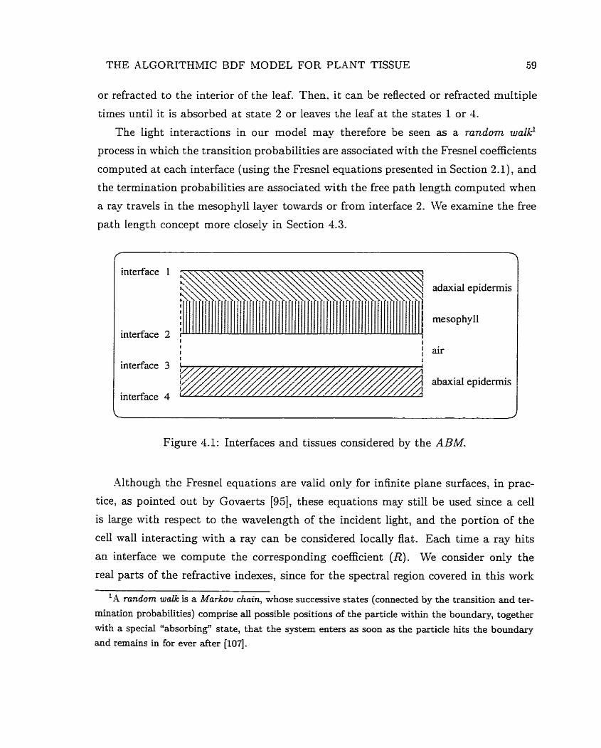
THE ALGORITHMIC BDF MODEL FOR PLANT TISSUE 59
or refracted to the interior of the leaf. Then, it can be reflected or refracted multiple
times until it is absorbed at state 2 or leaves the leaf at the states I or 4.
The light interactions in our mode1 may therefore be seen as a random walk-'
process in which the transition probabilities are associated rvith the Fresnel coefficients
computed at each interface (using the Fresnel equations presented in Section 2 4 , and
the termination probabilities are associated with the free path length computed when
a ray travels in the mesophyli layer towards or from interface 2. \Ye examine the free
path Iength concept more closely in Section 4.3.
adaxial epiderrnis
mesophy Il
1 air
Figure 4.1: Interfaces and tissues considered by the ABM.
-4lthough the Fresnel equations are valid only for infinite plane surfaces; in prac-
tice, as pointed out by Govaerts [95], these equations may still be used since a ce11
is large with respect to the wavelength of the incident light, and the portion of the
ce11 wall interacting with a ray can be considered locally flat. Each time a ray hits
an interface rve compute the corresponding coefficient (R). We consider only the
real parts of the refractive indexes, since for the spectral region covered in this work
'-4 nindorn walk is a Markou chain, whose successive states (connected by the transition and ter-
mination probabilities) comprise ail possible positions of the particle within the boundary, together
with a special "absorbing" state, that the system enters as soon as the particle hits the boundary
and remains in for ever after [107].
THE ALGORTTHMIC BDF MODEL FOR PLAIT TISSUE 60
(400nm to 700nm). and for the materials considered, the cornples parts are so small
that they can be neglected [95, 96: 173. 2411.
Using these sirnplifjt-ing assumptions the equation used to compute the Fresnel co-
efficients at each interface- assuming unpolarized light [198], reduces to Equat ion 2.11.
Xfter computing the Fresnel coefficient at an interface- we generate a uniform random
number E [O, 11. If the randorn number F is smaller than or equal to the Fresnel
coefficient R. Ive generate a reflected ray F. o theNse we generate a refiacted ray
The reflected ray is obtained usîng the law of reflection (Equation 2.3). The refracted
ray is obtained using Snell's law (Equation 2.6).
The ABM takes into account the three components of the BDF of plant tissues:
surface reflectance, subsurface reflectance and trammittance. They are affected by the
surface roughness, the interna1 scat tering and the light absorption in the mesophyll
tissue. In the next sections we describe how we address these issues.
4.2 Scattering Profile
Brakke et al. [38] have noted that the scattering profile of a plant leaf can be
approximated by an exponentiated cosine function. We have used a similar approach
to simulate the distribution of the rays reflected or refracted at the foliar tissues.
A rough surface, like a leaf epidermis, can contain more than one distinct scale of
roughness. The contour of the epidermal malls represents large surface features with
respect to the wavelength of the incident Iight. The microdetails of the epiticular
waxes represent the small surface features relative to the wavelength of the incident
light . For the plant epidermis the large-scale roughness Nil1 dominate scattering in the
specular direction, as pointed out by Grant [97], and the small-scale roughness will
control scattering away from the specular direction. The epiticular waxes exhibit
a wide range of geornetric configurations, and their contribution to the overall re-
flectance is not as significant as the overall shape of the epidermal cells. For these
reasons we decided to concentrate our simulation efforts on the large scale features.
Govaerts et a l [96] have shown that the epidermal cells can be appro'rirnated by
oblate ellipsoids. An oblate ellipsoid has semi-axes al , a2 and as, with al = a2 and
THE ALGORITHlLIIC BDF MODEL FOR PLANT TISSUE 61
al > a3 [212]. For the plant cells -ive consider a 1 and a? as the axes in the plane of
the foliar tissues, with values corresponding to average radius of the cell. a,. Lnlike
the oblateness definition used bu Covaerts et al. we define the oblateness of the ce11
as *. The dimensions of the epidermal cells of several species of plants can be found a3
in the literature [33: 95; 1331.
To simulate the effects of the shape of the epiderrnai cells on the reflected rays
at the air-epidermal cells interface, we perturb the rays using a warping function
(Equat ion 4.1). This function corresponds to a PDF based on an exponentiated cosine
distribution (Xppendix A)' and the exponent is given by the oblateness of the epi-
dermal cells. The perturbation is performed through angular displacements, a, and
Pe. The angle a, corresponds to the polar angle with respect to the ideai reflection or
ideal transmission direction. The angle Pe corresponds to the azimut ha1 angle around
the ideal reflection or ideal transmission direction. These angles are given by:
where:
ci and fZ = uniformly distributed random numbers E [O, 11,
ob = oblateness of the epidermal cells.
Therefore, Ieaves with large epidermal cells' oblateness will have a surface reflectance
closer to a specular distribution than leaves with srnall epidermal cells' oblateness. As
pointed out by Shirley [204], the energy conservation properties of a PDF based on
an exponentiated cosine function become Iess physical as the exponent gets smaller,
and the resulting behavior becomes that of a rnirror when the exponent becomes
larger. By associating this exponent with a biological meaninghil parameter, we set
boundaries for the values assumed by this exponent and, consequently, reduce the
chances of violating the energy conservation properties of this PDF. Based on the
dimensions of the epidermal cells for several species of plants found in the literature,
an appropriate range for the oblateness would be [1.4,5].
When light passes to the mesophyll its direction of travel is randomized and it
becomes diffuse. We simulate the distribution of the rays in this tissue using another
warping function (Equation 4.2). In this case the PDF corresponds to a diffuse
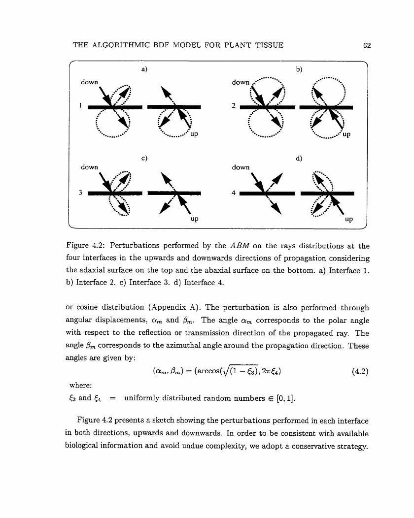
THE ALGORITHMIC BDF MODEL FOR PLANT TISSUE 62
down 4
down
Figure 4.2: Perturbations performed by the ABM on the rays distributions at the
four interfaces in the upwards and downwards directions of propagation considering
the adaxial surface on the top and the abaxial surface on the bottom. a) Interface 1.
b) Interface 2. c) Interface 3. d) Interface 4.
or cosine distribution ( Appendiu A). The perturbation is also performed through
angular displacements, a, and 0,. The angle cu, corresponds to the polar angle
with respect to the reflection or transmission direction of the propagated ray. The
angle 0, corresponds to the azimut hal angle around the propagation direction. These
angles are given by:
(%, Pm) = (arccos( Jm, 2rC*) (4-2)
where:
& and c4 = uniformly distributed randorn numbers E [O, 11.
Figure 4.2 presents a sketch showing the perturbations performed in each interface
in both directions, upwards and downwa.rds. In order to be consistent with available
biological information and avoid undue complexity, we adop t a conservative strategy.
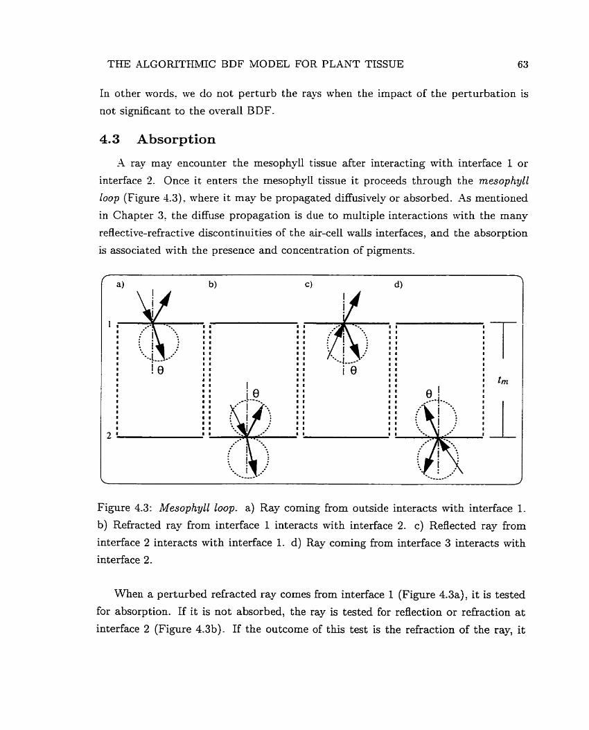
THE ALGORTTHNIIC BDF MODEL FOR PLANT TISSUE 63
In other words, we do not perturb the rays when the impact of the perturbation is
not significant to the overall BDF.
4.3 Absorption
-4 ray may encounter the mesophyll tissue after interacting with interface 1 or
interface 2. Once it enters the mesophyll tissue it proceeds through the mesophyll
loop (Figure 4.3): where it may be propagated diffusively or absorbed. -4s mentioned
in Chapter 3, the diffuse propagation is due to multiple interactions with the many
reflective-refract ive discontinuities of the air-ce11 walls interfaces, and the absorption
is associated with the presence and concentration of pigments.
Figure 4.3: Mesophyll loop. a) Ray coming from outside interacts vi th interface 1.
b) Refracted ray from interface 1 interacts with interface 2. c) Reflected ray from
interface 2 interacts with interface 1. d) Ray coming from interface 3 interacts mith
interface 2.
When a perturbed refracted ray cornes from interface 1 (Figure 4.3a), it is tested
for absorption. If it is not absorbed, the ray is tested for reflection or refiaction a t
interface 2 (Figure 4.3b). If the outcome of this test is the refraction of the ray, it
THE ALGORITHMIC BDF MODEL FOR PLANT TISSUE 64
is perturbed and transmitted to interface 3, othenvise the reflected ray is perturbed
and tested for absorption. If it is not absorbed, it may be reflected back to the
mesophyll a t interface 1 (Figure 4.3c), restarting the mesophyll loop, or refracted to
the environment.
FVhen a ray cornes from interface 3 (Figure 4.3d). it is also tested for reflection or
refraction a t interface 2. If the outcome of the test is a reflected ray, it is perturbed and
sent back to ioterface 3 without accounting for absorption. Othenvise, the refiacted
ray is perturbed and tested for absorption. If the ray is not absorbed, it proceeds in
the mesophyll loop.
The absorption of light in dye solutions varies with the thickness of the sample
and the concentration of pigments in accordance with a combination of Beer's law and
Bouguerk law (Section 2.3). This combination, however, assumes that the incident
ray- is perpendicular to the interface between the incident medium and the transmis-
sion medium. Allen e t al- [4] have included an additional term to this combination
to account for different angles of incidence. The resulting expression states that the
transmissivity of a plate along a slant ray is given by:
where:
44 C
h
8
absorption coefficient,
concentration of pigment,
thickness of plate,
angle of slant ray with respect to normal direction.
The absorption testing performed by the ABM is based on Equation 4.3, and
assuming a homogeneous distribution of pigments. It is performed probabilistically
every time a ray starts a run in the mesophyll tissue. It consists of the estimation of
the ray geometrical path length2, p, through the following expression:
*In this context the ray geometrical path length represents the spatial distance covered by a slant
ray transmitted through a medium until it is absorbed or Ieaves the medium.
THE ALGOFUTHMIC BDF MODEL FOR PLANT TISSUE
1 p = -- ln(<) cos O a= (4
where:
< = uniformly distributed random number E [O' 11 a, (A) = effective absorption coefficient of pigments,
O = angle between the ray direction and the normal direction.
The effective absorption coefficient. as described by Jacquemoud and Baret [125]
is given by:
ai(X) = specific absorption coefficient of a given pigment i (s), G = concentration of a given pigment i (2).
If p is greater than the thickness of the pigmented medium, t, (both expressed in
n): then the ray is propagated: otherüvise it is absorbed. The thickness value used
in this comparison does not correspond to the total thickness of the leaf, but to a
fraction of it. Since the palisade tissue presents a higher concentration of pigments
thao the spongy tissue, and it is largely responsible for the interna1 scattering, we
suggest to use its thickness (around 45% of the total thickness) for most cases. For
species t hat present an undifferentiated mesophyll tissue, e-g. characterized by the
presence of spongy cells only [81, 2301, we suggest using the entire thickness of the
mesophyll tissue (around 73% of the thickness).
A comprehensive set of leaf optical experiments, called L OPEX [120], provides
the pigment concentrations and thickness values for 120 leaf samples representative
of more than fifty species. The absorption spectra of chlorophyll and carotenoids
pigments can be found in the literature [34, 43, 53, 66, 125, 187, 193, 228, 247, 2481.
FVe examine this issue in more detail in Section 4.5.2. Additional information on
optical parameters of foliar tissues is available in a survey by Gausman and Allen [81].
THE ALGOFUTHMIC BDF MODEL FOR PLANT TISSUE 66
4.4 Implementation Overview and Summary of Parameters
The ABM was irnplemented using the C++ language and the ggLibrary [202],
a set of C++ utilities designed to be used in computer graphics applications. Ln
the ggLibrary materials are classified as families, such as metals and dielectrics, and
grouped by parameters that affect t heir behavior, following the ray tracing framework
for global illumination proposed by Shirley et al. [200]. A set of routines specific for
each family computes the BDF for that family.
In the case of the ABM, the new family corresponds to the pIant tissues: and each
of its four states is implemented through a different routine. These routines are called
recursively by a controlling routine until the ray is either absorbed or abandons the
foliar tissues, The parameters used in the ABM are the following:
vc - refractive indes of the external cutinized wall of the epidermis: used in the
Fresnel computations in states 1 and 4;
ob - oblateness of epidermal cells: used in the perturbation of the rays in state 1
(Figure 4.2a), in state 3 (Figure 4.2~): and in state 4 (Figure 4.2d);
vm - refractive index of the mesophyll ce11 wall: used in the Fresnel computations
in state 2
t , - thickness of mesophyll tissue: used in the absorption testing perfomed in
state 2 ( measured in cm);
c - concentration of pigments: also used in the absorption testing performed in
state 2 (measured in 5);
7. - refractive index of the antidermal wall: used in the Fresnel computations
in state 3.
The refractive indexes corne from experiments described in the literature [82, 125,
2411. The remaining parameters are also available in the literature, as mentioned
earlier. The user may also adjust the optical parameters, e-g. tm, depending on the
conditions a t hand. For example, for some species, a leaf in the sunlit and a leaf in
the shady portions of a tree, rnay present differeuces of thickness of around 25% [3].
THE ALGORITHMIC BDF MODEL FOR PLANT TISSUE 67
Notice that we use the same parameters for the adaxial and abaxial epidennis. This
approach is accurate for most cases, but for some species it may be more appropriate
to use a set of parameters with slightly different values.
We use the absorption spectra of chlorophyll a and b provided by Jacqueznoud
and Baret [125] in the absorption computations. Although these curves refer to
pigments comrnonly present in the foliar tissues of most species, they may be adjusted
according to the lengthening of the optical path of a given plant leaf. also called
ratio of intensification [43] or factor of intensification [183]. This factor represents
a combination of light that passes through plant tissues mithout encounterïng an
absorber (sieve effect) and the light that is scattered and haç an increased path
length (detour effect). As mentioned by Vogelmann [229], these two phenomena have
opposite outcornes: the sieve effect lowers absorption (specially at or near wavelengths
for which the absorption has a maximum value), whereas the detour effect increases
absorption (specially a t or aear wavelengths for vvhich the absorption has a minimum
value). Nonetheless, in dispersive samples, such as plant leaves, the absorption is
enhanced by the combination of these two effects [183].
The factor of intensification of a plant leaf depends on the chlorophyll content.
The greater the chlorophyll content, the shorter the length of the optical path. For
example, McCleudon and Fukshansky [la71 made estimates of factors of intensification
for plant leaves of nine different species with a chlorophyll content between 40 and
7 0 3 , and the resulting value, i -e . the mean and the standard deviation, was 2.30 I
0.25.
4.5 Testing Issues
One possible approach for validating a BDF mode1 is visual inspection by compar-
ing images generated using the mode! with images generated using previous models.
This approach is not suitable in our case, since the graphics literature lacks models
aimed at plants. Recall that, although the multiple-layer model proposed by Hanra-
han and Krueger [IO91 can be applied to plants (Section 2.6.3), it does not compute
the reflectances and transmittances by itself, which are introduced to the model as
THE ALGORITHMIC BDF MODEL FOR PLANT TISSUE 68
input parameters. Therefore. comparing such a model with the -4BM, rvhich actually
computes the reflectances and transmit t ances3, is not appropriate.
Another alternative would be to compare images generated using the ABM with
photographs of real plants. In this case- since the computer generation of images
is highly dependent on rendering parameters, the validation of the ABM could be
biased b - errors generated by other stages of the rendering pipeline, such as geomet-
rical modeling, spectral modeling and directionai sampling. As appropriately stated
by Dekbung and Fournier [ 6 / ] , the shape of a n object, the lighting, and the viewing
position c m al1 greatly affect how much BDF properties affect an image, and at-
ternpting to measure how much effect these properties wiviil have on generated images
would necessitate a separate investigation.
Since our goal at this point of our research is not necessarily to generate the best
possible image of a plant, but to contribute to its synthesis respecting the laws of
physicsl we chose to test our model as a separate unit of the rendering pipeline and
compare the results with the best available experimental data. In order to perform
a comprehensive validation of a BDF model it would be necessary to consider al1
possible illuminating and viewing geometries. The wry large number of measurernents
needed as well as the lack of e?rperimental data for all possible geometries precludes
the use of this approach.
Judd and Wyszecki [128] pointed out that in many goniophotometric measure-
ments the most interesting and informative data for practical sarnples are taken in
the plane given by the direction of the incident light and the normal of the spec-
irnen. Therefore, due to the practical reasons mentioned above and the isotropie
characteristic of the ABM, we chose to use this plane in its testing.
4.5.1 Simulation of Devices for Measurement of Appearance
We are interested not only in the spectrophotometric curves of reflectance, p,
and transmittance, T , but also in the goniophotometric BDF curves, given in terms
of BRDF, f,, and BTDF, ft. The spectrophotometric measurements are taken to
3The reflectances and transmittance computed by the ABM can be used as input parameters
by other models, including, but not limited to the 8-K multiple-layer model. We examine this
possibility in more detaii in Chapter 6.
THE ALGORITHMIC BDF MODEL FOR PLANT TISSUE 69
determine the spectral energy distribution of the propagated light and the gonio-
photometric measurements are made to find the spatial distribution of that light-
As mentioned in Section 2.5. while tbese two groups of measurements can be per-
formed separately. they work together to establish the measurement of appearance of
an object (Section 2.5).
Xctual measurements of p and T are performed using spectrophotorneters4 equipped
with an integrating sphere, and the actual measurements of fr and ft are performed
using goniophotometers (122, 1281. These devices are important basic tools for fun-
damental research in colorimetry [l5 11, solar engineering [Pl] ; rernote sensing [63] and
plant biochemistry [34].
An integrating sphere is usually used to measure the hemispherical reflectance
factor, which is defined as the ratio of the BILX reflected by a sample under speci-
fied conditions of irradiation and collection to that reflected by the ideal completely
reflecting isotropically diffusing surface under identical conditions of irradiation and
viewing [246]. However, the numerical values of reflectance (Section 2.2) and re-
flectance factor are identical under the conditions of hemispherical collection [86].
For absolute measurements, the sphere wall is the standard, and the integrat-
ing sphere theory [87] compensates for the absolute reflectance of the sphere wall by
mathematically treating the wall reflectance as unity. Hence, as pointed out by Zer-
laut and Anderson [246], the hemispherical measurements made Mth such integrating
spheres are the absolute reflectance (or the absolute transmittance) subject to small
errors associated with aperture losses, small values of non-uniformity of sphere wall
reflectance, sample mounts and so on.
Besides the BDF computations, the measurernent of light distributions of speci-
mens performed by goniophotometers also allows the verification of reciprocity and
anisotropy properties of these specimens. Moreover, this device can also be used to
measure the glossiness (Section 2.5) of a specimen given by its gloss factor. In this
case the measurement is made relative to a perfect mirror surface instead of a perfect
diffuser surface [128].
4The spectrophotometers can also be used to determine the absorption characteristics of a spec-
imen as a function of wavelength [161].
THE ALGORITHMIC BDF MODEL FOR PLANT TISSUE 70
The reflectance, transmittance and BDF measurements for testing purposes de-
scribed in this dissertation were performed using computer simulations of a spec-
trophot omet er and goniopho tometer, hencefort h called virtual measurement devices.
The use of such virtual devices gives us control over the spectral data generation
and allows us to capture a BDF at different sampling resolutions as pointed out by
Lalonde and Fournier [141]. Moreover. it also allows us to avoid measurernent er-
rors such as perturbations in the incident and viewing angles due to the fact that
specimens tend not to lie flat on the specimen holders of real rneasurement devices.
In our simulation of a spectrophotometer with integrating sphere the rays are
shot from an emitter placed above the specimen following an incident solid angle:
2. Considering a total number of iV rays fired towards the specimen for a given
wavelength A, one can assume that each ray carries the same amount of pon-er, a. If the total power to be shot is <Pi, then, as stated by Shirley [198, 2001, the power
carrïed by each ray is given by:
Recall that reflectance describes the ratio of reflected power to incident power, and
transmittance describes the ratio of transmitted power to incident power. Considering
this ratio, if rn, rays are reflected towards the upper hemisphere, Q,, the spectral
reflectance of the specimen with respect to a given wavelength X of the incident light
WU be given by:
Therefore, since we can simply count the number of rays reflected to the upper
hemisphere to determine a specimen7s absolute spectral reflectance, we do not need
to use an integrating sphere in our virtual spectrophotometer in order to collect the
reflected rays. The absolute spectral transmittance is calculated similarly considering
the lower hemisphere.
In our simulation of a goniophotometer we use a slightly difFerent arrangement.
Instead of considering the entire upper and lower hemisphere as collectors, we use
THE ALGORITHMIC BDF MODEL FOR PLANT TISSUE 71
several radiance detectors represented by the patches of a collecter sphere placed
around a specimen. Csing this arrangement: the BRDF regarding a direction associ-
ated with a given radiance detector placed in the upper hemisphere is determined in
ternis of radiant power. More spe~ifically~ it is given by the ratio between the radiant
power reaching the detector? a': after interacting with the specimen, and the incident
radiant power, a' [17: 951.
The corresponding expression used to compute the BRDF for light incident at
wavelength A: considering the solid angle regarding the direction of incidence, & and
the solid angle regarding the direction associated Mth
aven by:
the radiance detector, w',, is
where:
GP = projected solid angle regarding the direction associated with the
radiance detector.
In turn: the projected solid angle GP is given by:
where:
d-4,. = area of the radiance detector,
L = distance from the specirnen to the radiance detector,
$7- = angle between the direction associated with the radiance detector and the specimen normal.
Recall that the radiant power reaching the radiance detector can be written as:
Thus, replacing Equation 4.6 and Equation 4.10 in Equation 4.8, the expression to
compute the BRDF reduces to:
THE ALGOFUTKWC BDF MODEL FOR PLANT TISSUE 72
Similarly, the BTDF is calculated considering radiance det ect ors placed in the lower
hemisp here.
The origins of the rays are random points uniformly chosen from a disk used
to represent the surface of the emitter. The coordinates of the points are given by
the pair (O: Z) , which is computed using the following warping function suggested by
Shirley [198]:
where:
Ci and & = uniformly distributed random numbers E [O. 11.
R = radius of the disk.
The targets of the rays are random points uniformly chosen from a pair of triangles
used to represent the specimen. To choose a random point q on a triangle defined by
the vertices q ~ ; ql and 92 we use the following expression:
where p and 7 are obtained using another warping function suggested by Shirley
[ N B ] :
(P: 7) = (1 - ,/l - t37 (1 - P)&)
where:
c 3 and c4 = uniformly distributed random numbers E [O, 11.
The precision of real rneasurement devices is estimated by the ability of the in-
strument to repeat a measurement of a given specimen as mentioned by Judd and
Wyszecki [128]. For instance, a spectrophotometer is considered to be of high preci-
sion if the spectral measurement , reflectance or transmittance, is repeated to achieve
a tolerance better than b ( X ) = f 0.001. In our simulations we select the number of
rays N to be shot using this tolerance value to avoid undesirable fluctuations in the
measurement S.
THE ALGOFUTHMIC BDF MODEL FOR PLANT TISSUE 73
4.5.2 Testing Parameters
The set of leaf optical experirnents cited in Section 4.3? LOPEX [120], includes
measured spectral curves of reflectance and transmittance. In order to compare our
resul ts with these measured Cumes? we attempt to reproduce the actual mea-surement
conditions used in the L OPEX as faithfully as possible. We use the same area for the
specirnen, 40mm2, and the same angle of incidence, 8": with respect to the normal of
the specimen. Our emitter has a radius of 8mm, and it is positioned a t a distance of
30mm from the center of the specimen. Shese values correspond respectively to the
area of the apertures and radius of the integrating sphere of the spectrophotometer
used by LOPEX
We selected, without loss of generality, a leaf from the soya species (Glycine max,
Soja hispida), cornmonly k n o m as a soybean leaf: because of its standard foliar
characteristics and the large variety of experirnental data available for comparison
[do, 98, 100. 120, 156, 232, 2401 besides LOPEX. The parameters used in our testing
experirnents are presented in Table 4.1. The refractive indexes were obtained from
the ivork by Wooley [241], and the oblateness corresponds to the average dimensions
of the epidermal cells of plant leaves belonging to the dicotyledons group (a, = 12.5,
a3 = 2.5), which are available in the texts by Govaerts et al. [96] and Norman [172].
Table 4.1: Parameters used in the testing of the ABM.
The concentration of chlorophyll was obtained directly from LOPEX, and the
thickness was cornputed using 45% of the total soybean leaf thickness, also provided by
LOPEX, as proposed in Section 4.3. The cornbined absorption spectra of chlorophylls
a + 6 used in the testing of the ABM (Figure 4.4) is based on the curve provided by
Jacquemoud and Baret [125], but adjusted according to a factor of intensification of
2.13 [157, 1831 and values of free path length (Section 4.3) given in m.
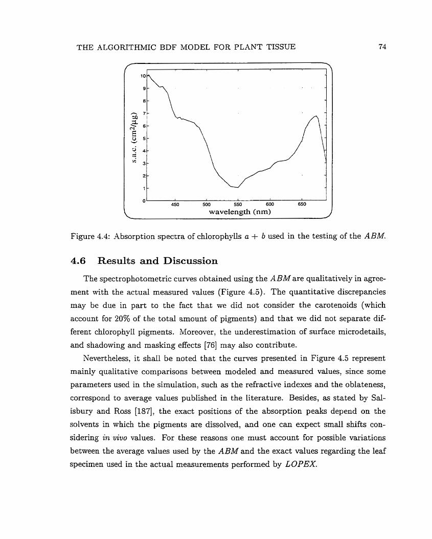
THE ALGORITHMIC BDF MODEL FOR PLANT TISSUE
wavelength (nm)
Figure 4.4: Absorption spectra of chlorophylls a + b used in the testing of the ABM.
4.6 Results and Discussion
The spectrophotometric curves obtained using the A BM are qualitatively in agree-
ment with the actual measured values (Figure 4.5). The quantitative discrepancies
may be due in part to the fact that we did not consider the carotenoids (which
account for 20% of the total amount of pigments) and that Ive did not separate dif-
ferent chlorophyll pigments. Moreover, the underestimation of surface microdetails,
and shadowing and masking effects [76] may also contribute.
Nevertheless, it shall be noted that the curves presented in Figure 4.5 represent
mainly qualitative comparisons between modeled and measured values; since some
parameters used in the simulation, such as the refractive indexes and the oblateness,
correspond to average values published in the literature. Besides, as stated by Sal-
isbury and Ross [187], the exact positions of the absorption peaks depend on the
solvents in which the pigments are dissolved, and one can expect srna11 shifts con-
sidering in vivo values. For these reasons one must account for possible variations
between the average values used by the ABM and the exact values regarding the leaf
specimen used in the actual measurements performed by LOPEX.
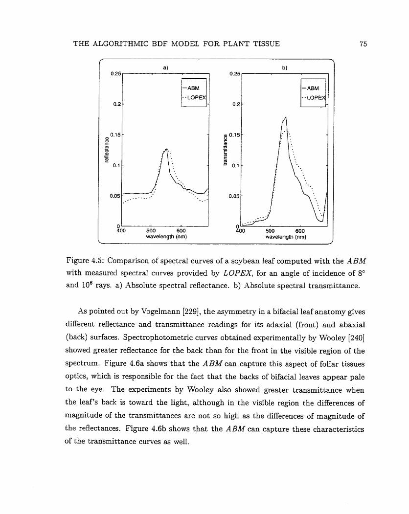
THE ALGORITHPvIIC BDF MODEL FOR PLANT TISSUE
- - LOP d'
O 400 500 600
wavelength (nm) wavelength (nm)
Figure 4.5: Cornparison of spectral curves of a soybean leaf computed with the ABM
with rneasured spectral curves provided by LOPEX, for an angle of incidence of 8"
and 106 rays. a) Absolute spectral refiectance. b) Absolute spectral transmit tance.
As pointed out by Vogelmann [229], the asymmetry in a bifacial leaf anatomy gives
different reflectance and transmittance readings for its adaxial (front) and abaxial
(back) surfaces. Spectrophotometric curves obtained experimentally by Wooley [240]
showed greater reflectance for the back than for the front in the visible region of the
spectrum. Figure 4.6a shows that the ABM can capture this aspect of foliar tissues
optics, which is responsible for the fact that the backs of bifacial leaves appear pale
to the eye. The expenments by Wooley also showed greater transmittance when
the leaf's back is toward the light, although in the visible region the differences of
magnitude of the transmittances are not so high as the differences of magnitude of
the reflectances. Figure 4.6b shows that the ABM can capture these characteristics
of the transmittance curves as well.
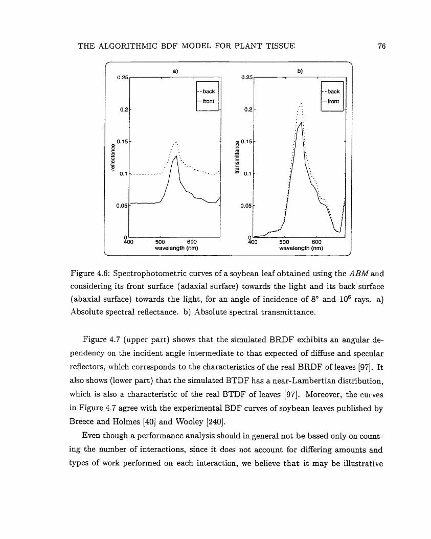
THE ALGOEUTHMIC BDF MODEL FOR PLANT TISSUE
a) O -25
- - back
-front 0.2 - C
wavelength (nm)
l--L 0- 400 500 600
wavelength (nm)
Figure 4.6: Spectrophotometnc curves of a soybean leaf obtained using the ABM and
considering its front surface (adaxial surface) towards the light and its back surface
(abaxial surface) towards the light, for an angle of incidence of 8" and 106 rays. a)
Absolute spectral reflectance. b) Absolute spectral transmittance.
Figure 4.7 (upper part) shows that the simulated BRDF exhibits an angular de-
pendency on the incident angle intemediate to that expected of d i f i se and specular
reflectors, which corresponds to the characteristics of the real BRDF of Ieaves [97]. It
also shows (lower part) that the simulated BTDF has a near-Larnbertian distribution,
which is also a characteristic of the real BTDF of leaves [97]. Moreover, the curves
in Figure 4.7 agree with the experimental BDF curves of soybean leaves published by
Breece and Holmes [40] and Wooley [240].
Even though a performance analysis should in general not be based only on count-
ing the number of interactions, since it does not account for differing amounts and
types of work performed on each interaction, we believe that it may be illustrative
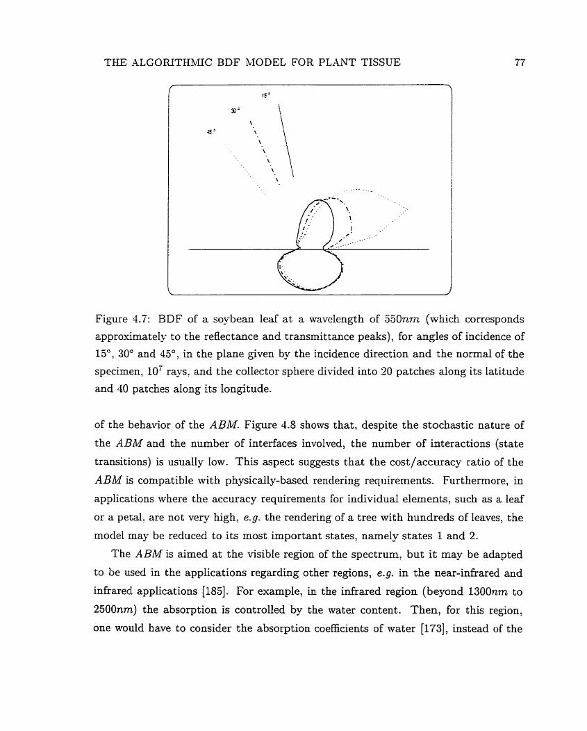
THE ALGORZTHMIC BDF MODEL FOR PLANT TISSUE
Figure 4.7: BDF of a soybean leaf at a wavelength of 5JOnm (which corresponds
approximateIy to the reflectance and transmittance peaks), for angles of incidence of
15", 30" and 45", in the plane given by the incidence direction and the normal of the
specimen; loi rays? and the collecter sphere divided into 20 patches along its latitude
and 40 patches along its longitude.
of the behavior of the ABM. Figure 4.8 shows that, despite the stochastic nature of
the ABM and the number of interfaces involved, the number of interactions (state
transitions) is usually low. This aspect suggests that the cost/accuracy ratio of the
ABM is compatible with physically-based rendering requirements. Furthemore, in
applications where the accuracy requirements for individual elements, such as a leaf
or a petal, are not very high, e.g. the rendering of a tree with hundreds of leaves, the
mode1 may be reduced to its most important states, namely states 1 and 2.
The ABM is aimed at the visible region of the spectrum, but it may be adapted
to be used in the applications regarding other regions, e.g. in the near-infrared and
infrared applications [185]. For example, in the infrared region (beyond 1300nm to
2500nm) the absorption is controlled by the water content. Then, for this region,
one would have to consider the absorption coefficients of water [173], instead of the
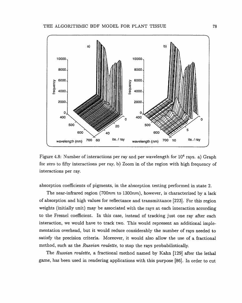
THE ALGORTTE1IUIIC BDF MODEL FOR PLANT TISSUE
wavelength (nm) 700 60 ite. / ray wavelength (nm) 700 ite. 1 ray
Figure 4.8: Number of interactions per ray and per wavelength for 104 rays. a ) Graph
for zero to fifty interactions per ray, b) Zoom in of the region with high frequency of
interactions per ray.
absorption coefficients of pigments, in the absorption testing performed in state 2.
The near-infrared region (700nm to 1300nm), however, is characterized by a lack
of absorption and high values for reflectance and transmittance [223]. For this region
weights (initially unit) may be associated with the rays a t each interaction according
to the Fresnel coefficient. In this case, instead of tracking just one ray after each
interaction, we would have to track two. This would represent an additional imple-
mentation overhead, but it would reduce considerably the number of rays needed to
satisfy the precision criteria. Moreover, it would also allow the use of a fractional
method, such as the Russian roulette, to stop the rays probabilistically.
The Russian roulette, a fractional method named by Kahn [129] after the lethal
game, has been used in rendering applications with this purpose [86]. In order to cut
,THE ALGORITHMIC BDF MODEL FOR PLANT TISSUE 79
down the number of particles (rays)? we select one whose weight is below some thresh-
old due to multiple bounces during the random walk. Shen we use some probability
P [62] to discard it (i. e. we say the particle is absorbed) or to allow it t o continue. In
the later case its weight is multiplied by (1 - P ) -'. This procedure can be repeated
(with the same or different values for P ) until the number of particles is reduced to
a manageable size [10'7].
4.7 Summary
In this chapter ive have presented a plausible and biologicall-based BDF model
for plant tissue. the ABM. This model is controlled by a small number of biologically
meaningful parameters and presents a cost/accuracy ratio that suffices for physically-
based rendering applications. We examine this issue in more detail in the next chap-
ters. Moreover, the ABM can easily fit into global illumination frarneworks due to its
simple formulation based on standard Monte Car10 rnethods.
Differently from other BDF models available in the cornputer graphics literature'
the ,4BM does not rely on inputed values of reflectance and transmittance. Indeed,
these values are computed by the ABM itself. This aspect and its design specifically
tailored to foliar tissues make its comparison ni th other models used in rendering
applications troublesome. The comparison of images generated using the ABM with
photographs of reai plants would not be appropriate either, since it could be biased
by errors introduced in other stages of the rendering pipeline. For these reasons, we
have tested it as a separate unit of the rendering pipeline through comparisons with
real measured data. In order to perform these comparisons we have irnplemented
virtual measurement devices.
Our simulations show that the spectral curves obtained using the ABM are in
good agreement with measured values. The surface reflectance readings provided
by the ABM may be improved through the simulation of wax configurations and
incorporation of shadowing and masking effects. Moreover, although there is little
experimental data on the anisotropy of plant tissues, the incorporation of factors
affecting it, such as the presence of venation and hair, could îurther improved the
spectral curves provided by the ABM.
THE ALGORITHMIC BDF MODEL FOR PLANT TISSUE 80
It is important to note that we did not perfonn an ad hoc adjustrnent of the
parameters to obtain the spectral curves through the ABM. In other words, we have
used values as close as possible to the red values associated with the specimen tested.
These values were obtained from the remote sensing and botany Iiterature. PVe have
also attempted to reproduce. as faithfull-y as possible, the real experïmental conditions
in nrhich the actual measured curves ivere obtâined.
In this chapter ive have also pointed out suggest.ions to improve the efficiency of
the ABM and to extend its range of applications. In the next chapters we examine
alternatives to reduce the computational costs involved in the simulations of light in-
teraction witith foliar tissues. We also compare the images obtained using the ditferent
proposed approaches, including the ABAL
A Nondeterministic Reconstruction Approach
The in-Iine application of a BDF model, such as the ABM may add a significant
computational overhead to the rendering process. For some applications, e.g. a scene
with many leaves with the same biophysicd characteristics, it is more convenient
to measure the BDF, store its values in memory and reconstruct it d u i n g rendering
saving valuable time. As mentioned in the previous chapter, the BDF of a surface can
be measured using a measurement device known as a goniophotometer, or through a
computer simulation of such a device, rvhich is called a virtual goniophotometer. In
both cases, a large number of measurements is usually required to represent the BDF
accurat ely.
Fortunately, we can often exploit some characteristics of materials and BDF mod-
els used in rendering applications to reduce the nurnber of measurements, without
decreasing the accuracy of the BDF curves provided by these models significantly. An
example is given by plant leaves. -4s mentioned in Chapters 3 and 4, currently there
is not enough information to support the design of a biologically-based anisotropic
BDF model for these materials. Therefore, since in practice we are working with an
isotropic BDF model, we need to use only one directional input parameter, which
reduces the number of measurements considerably.
In this chapter an approach to reconstruct isotropic BDFs is presented. It consists
of pre-computing the BDF for a given material uçing an appropriate BDF model, and
storing its corresponding spectral and directional values. Afterwards, these values are
used to reconstruct the BDF during rendering. Instead of applying a deterministic'
this conteut we use the terms deterministic and nondeterministic according to how the dif-
ferent approaches select the PDF used to generate the outgoing distribution of rays associated with
a given BDF.
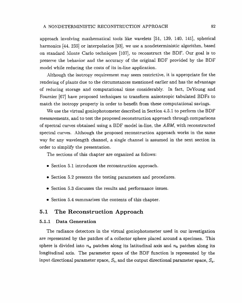
A NONDETERMINISTIC RECONSTRUCTION APPROACH 82
approach involving mathematical tools like wavelets [S. lo 139: 140: 1111 : spherical
harmonies [U. 2331 or interpolation [93]: we use a nondeterministic algorithm? based
on standard Monte Carlo techniques [107], to reconstmct the BDF. Our goal is to
presen-e the behavior and the accuracy of the original BDF provided by the BDF
model while reducing the costs of its in-line application.
.Ut hough the isotropy requiremeat may seem restrictive, it is appropriate for the
rendering of plants due to the circumstances mentioned earlier and has the advantage
of reducing storage and computational time considerably In fact, DeYoung and
Fournier [67] have proposed techniques to transform anisotropic tabulated BDFs to
match the isotropy property in order to benefit from these computational savings.
We use the virtud goniophotometer described in Section 4.5.1 to perform the BDF
measurements, and to test the proposed reconstruction approach t hrough cornparisons
of spectral curves obtained using a BDF model in-line: the ABM, with reconstructed
spectral curves. Although the proposed reconstruction approach works in the same
way for any wavelength channel, a single channel is assumed in the next section in
order to simplify the presentation.
The sections of this chapter are organized as follows:
Section 5.1 introduces the reconstruction approach.
Section 5.2 presents the testing parameters and procedures.
Section 5.3 discusses the results and performance issues.
Section 5.4 summarizes the contents of this chapter.
5.1 The Reconstruction Approach
5.1.1 . Data Generation
The radiance det ectors in the virtual goniophotometer used in our investigation
are represented by the patches of a collecter sphere placed around a specimen. This
sphere is divided into na patches along its latitudinal axis and nb patches along its
longitudinal axis. The parameter space of the BDF function is represented by the
input directional parameter space, Si, and the output directional paramet er space, S,.
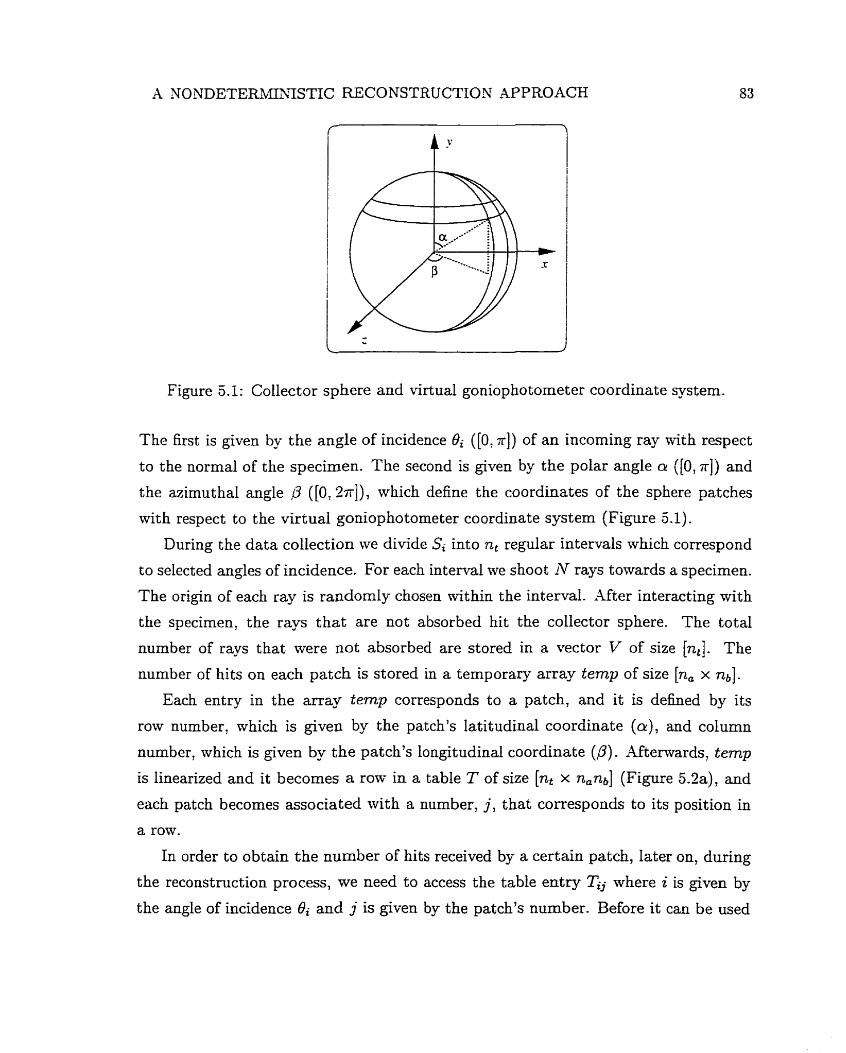
A NONDETER~IIL'NISTIC RECONSTRUCTION APPROACH
Figure 3.1: Collect or sphere and virtual goniophotometer coordinate system.
The first is given by the angle of incidence Bi ([O, T]) of an incoming ray with respect
to the normal of the specimen. The second is given by the polar angle <Y ([O, T I ) and
the azimuthal angle ,i3 ([O: %TI), which define the coordinates of the sphere patches
nrith respect to the virtual goniophotometer coordinate system (Figure 3.1).
During the data collection we divide Si into nt regular intervals which correspond
to selected angles of incidence. For each interval we shoot N rays towards a specimen.
The origin of each ray is randornly chosen within the interval. After interacting with
the specimen, the rays that are not absorbed hit the collecter sphere. The total
number of rays that were not absorbed are stored in a vector V of size [nt]. The
number of hits on each patch is stored in a temporary array temp of size [na x nb].
Each entry in the array temp corresponds to a patch, and it is defined by its
row number, which is given by the patch's latitudinal coordinate (a), and colurnn
number, which is given by the patch7s longitudinal coordinate (O). -Utemards, temp
is linearized and it becomes a rom- in a table T of size [Q x n,nb] (Figure 5.2a), and
each patch becomes associated with a number, j, that corresponds to its position in
a row.
In order to obtain the number of hits received by a certain patch, later on, during
the reconstruction process, we need to access the table e n t v Tij where i is given by
the angle of incidence Bi and j is given by the patch's number- Before it can be used
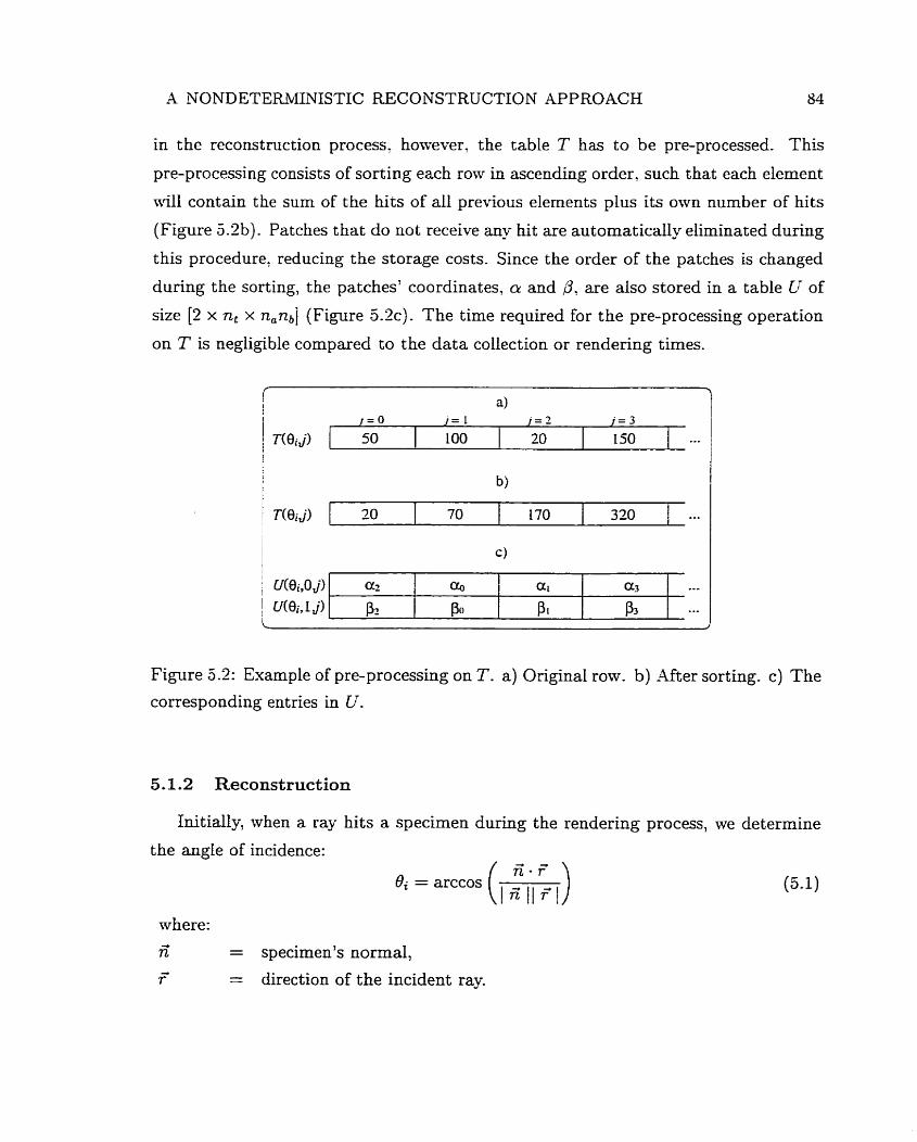
A NONDETEFtblINISTIC RECONSTRUCTION APPROACH 84
in the reconstruction process, howet-er. the table T has to be pre-processed. This
pre-processing consists of sorting each row in ascending order, such that each element
ni11 contain the sum of the hits of al1 previous elements plus its own nurnber of hits
(Figure 3 .a). Patches t hat do not receive an-- hit are automatically eliminated dunng
this procedureo reducing the storage costs. Since the order of the patches is changed
during the sorting, the patches' coordinates, ar and P , are also stored in a table U of
size [2 x nt x nanb] (Figure 5 2 ) . The time required for the pre-processing operation
on T is negligible compared to the data collection or rendering times.
Figure 5.2: Example of pre-processing on S. a) Original row. b) After sorting. c) The
corresponding entries in U.
5.1.2 Reconstruction
Initially, when a ray hits a specimen dunng the rendering process, we determine
the angle of incidence: 5 - 7
Bi = arccos (, ) fi Il r ' l
where:
5 = specimen's normal,
r' = direction of the incident ray.
-4 NONDETERMiN?STIC RECONSTRUCTION APPROACH 85
Then. we generate a uniformly distributed random number < E [O, NI. If this
random number E is greater than the number of non-absorbed rays stored in V(Bi) we
proceed to the neln ray: saving valuable time. Othenvise, we proceed to the kernel of
the algorit hm. where the reconstruction of the BDF takes place.
In the kernel we perfom a search in the array T to determine the smallest
T(Oi, j ) > E. In this way the elements associated with the largest numbers of hits
will have the highest probabilities of being selected. Once we determine the rom ele-
ment T(&, j ) : we use j to obtain the patch's coordinates a. and ,O stored in U(Bi7 0: j )
and U(Oi, 1' j ) respectivek Then the direction of the outgoing ray is given by the
angles a, and 13,:
where:
Ci and G = uniformly distnbuted random numbers E [O? 11.
These angles: in tum, correspond to aogular displacements with respect to the
g-axis and the z-axis of the virtual goniophotometer coordinate systern (Figure 5.1).
Considering t hat the incident rays are generated during the rendering using a different
coordinate system, namely the coordinate system associated with a virtual camera,
the generation of the outgoing ray has to be preceded by an appropriate coordinate
system transformation ('753.
5.1.3 Searching
The searching process mentioned above can be performed using binary search,
which has a worst case cost of L~!og~(n,n~)J + 1 comparisons. However, initial ex-
periments showed that this strategy was not fast enough for our application. We,
therefore, decided to use instead a hashing technique in which the colurnn indexes of
T are mapped to another table H of size [nt x G] (Figure 5.3a).
For an entry of T represented by T(i, j) the mapping is performed using the
following approach:
H(i7v ) = j (5-3)
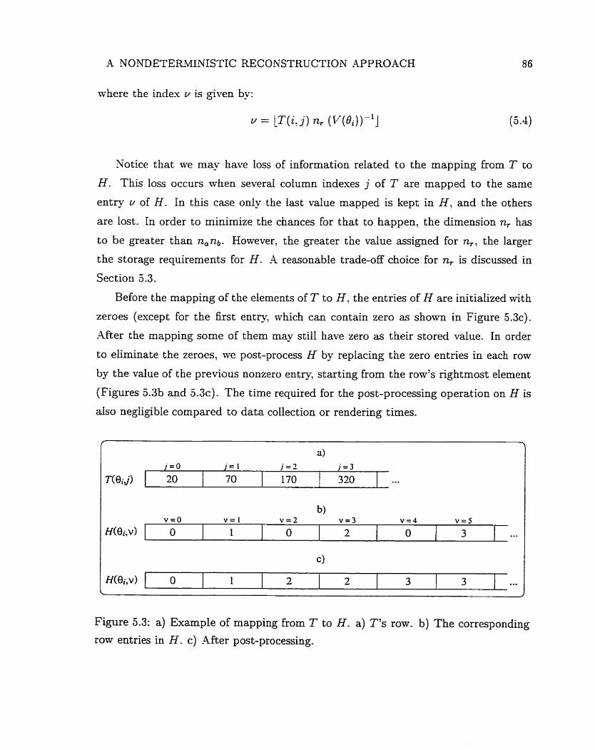
A NONDETERMINISTIC RECONSTRUCTION APPROACH
where the index v is giwn by:
u = iS(i. j ) n, (V(Bi))-'J
Notice that we may have Ioss of information related to the mapping from T to
H. This loss occurs mhen several column indexes j of T are mapped to the same
entry u of H . In this case only the last value mapped is kept in H ! and the others
are lost. In order to minimize the chances for that to happen, the dimension n, has
to be greater than n,nb. However: the greater the value assigned for n,; the larger
the storage requirements for H . A reasonabie trade-off choice for n, is discussed in
Section 5.3.
Before the mapping of the elements of T to H , the entries of H are initialized with
zeroes (except for the first entry, which can contain zero as shown in Figure 5.3~) .
After the mapping some of them may still have zero as their stored value. In order
to eliminate the zeroes, we post-process H by replacing the zero entries in each row
by the value of the previous nonzero entry, starting £rom the row's rightmost element
(Figures 5.3b and 5 . 3 ~ ) . The time required for the post-processing operation on H is
d s o negligible compared to data collection or rendering times.
Figure 5.3: a) Example of mapping from T to H. a) S's row. b) The corresponding
row entries in h-. c) After post-processing.
,4 XONDETERMINISTIC RECONSTRUCTION APPROACK 87
During the reconstruction. we use table H instead of table T . to access the coor-
dinates of a patch associated with <. The patchTs position in U is stored in H(Oi: y)'
and the index v is computed using the following expression:
5.2 Testing Parameters and Procedures
The data used in our testing esperiments corresponds to a soybean leaf's BDF,
mhich was computed using the ABM (Chapter 3)- The coliector sphere used by the
virtual goniophotometer was divided into 20 patches along its latitudinal
(na = 20) and 40 patches along its longitudinal axis (nb = 40). The d a t a collec-
tion was performed in intervals of 1" for Si (nt = 180). The testing measurements
were made using 10% incident rays per interval, and considering the plane given by
the incident light and the specimen's normal.
Lilley et al. [148] mention that to provide the correct color in high quality com-
puter graphies, the CIE XYZ values should be converted to the RGB color space
of a monitor using the SMPTE2 monitor chromaticity coordinates. In fact, many
monitors used in the current workstations use these coordinates. Thus, we decided
to sample the absorption spectra of chlorophyll (Figure 4.4) in the dominant wave-
lengths corresponding to these coordinates (Table 5.1) in order to generate the cunres
and the images presented in the next section. Note that the dominant wavelength
regarding the green channel corresponds approximately to the wavelength for which
the absorption of light by chlorophyll is minimum (Figure 4.4).
,Y y wavelengt h
Red 0.630 0.340 608nm
Green 0.310 0.595 551nrn
Blue 0.155 0.070 455nm
white (D65) 0.313 0.329
Table 5 -1 : Chromaticity coordinates and wavelength values.
'Society of Motion Picture and Television Engineers.
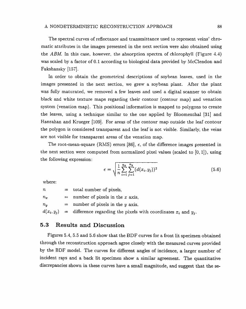
A NONDETERMINXSTIC FU3CONSTRUCTION APPROACK 88
The spectral curves of reflect ance and transmitt ance used to represent veins' chro-
matic attributes in the images presented in the next section were also obtained using
the ABM. In this case. hoivever, the absorption spectra of chlorophyll (Figure 4.4)
\vas scaled by a factor of 0.1 according to biological data provided by McClendon and
Fukshanslq [lu].
In order to obtain the grometrical descriptions of soybean leaves, used in the
images presented in the next section, we gresv a soybean plant. After the plant
\vas full- maturated. we removed a fem leaves and used a digital scanner to obtain
black and white texture maps regarding their contour (contour map) and venation
system (venation map). This positional information is mapped to polygons to create
the leaves, using a technique similar to the one applied by Bloomenthal [31] and
Hanrahan and Krueger [log]. For areas of the contour map outside the leaf contour
the polygon is considered transparent and the Ieaf is not visible. Similarly, the veins
axe not visible for transparent areas of the venation map.
The root-mean-square (RMS) errors [86], E , of the difTerence images presented in
the
the
nest section were computed from normalized pixel values (scaled to 0 : I I ) , using
following expression: 1 7 nr n~
where:
n = total ~ u m b e r of pixels,
nz = number of pixels in the x axis,
n~ = number of pivels in the y &es,
d(x i , yj) = difference regarding the pixels with coordinates xi and y j .
5.3 Results and Discussion
Figures 5.4,5.5 and 5.6 show that the BDF curves for a front lit specimen obtained
through the reconstruction approach agree closely with the measured curves provided
by the BDF model. The c w e s for different angles of incidence, a larger nurnber of
incident rays and a back lit specimen show a similar agreement. The quantitative
discrepancies shown in these curves have a small magnitude, and suggest that the se-
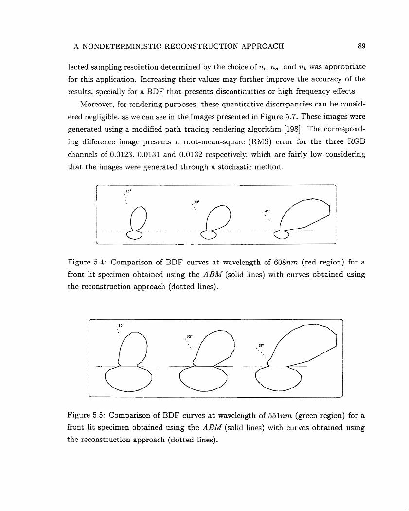
A NONDETERMINISTIC RECONSTRUCTION APPROACH 89
lected sampling resoiution determined by the choice of nt , na, and nb was appropriate
for this application. Increasing their values may further improve the accuracy of the
results. specially for a BDF t hat presents discontinuities or high frequency effects.
14 oreover, for rendering purposes, t hese quantitative discrepancies can be consid-
ered nepligible. as rve can see in the images presented in Figure 5.7. These images were
generated using a modified path tracing rendering algorithm [19S]. The correspond-
ing difference image presents a root-mean-square (RMS) error for the three RGB
channels of 0.0123: 0.0131 and 0.0132 respectively, which are fairly low considering
that the images were generated through a stochastic method.
Figure 5.4: Comparison of BDF curves at wavelength of 608nm (red region) for a
front lit specimen obtained using the ABM (solid lines) with curves obtained using
the reconstruction approach (dotted lines).
Figure 5.5: Comparison of BDF curves at wavelength of 551nm (green region) for a
front lit specimen obtained using the ABM (solid lines) with curves obtained using
the reconstruction approach (dotted lines).
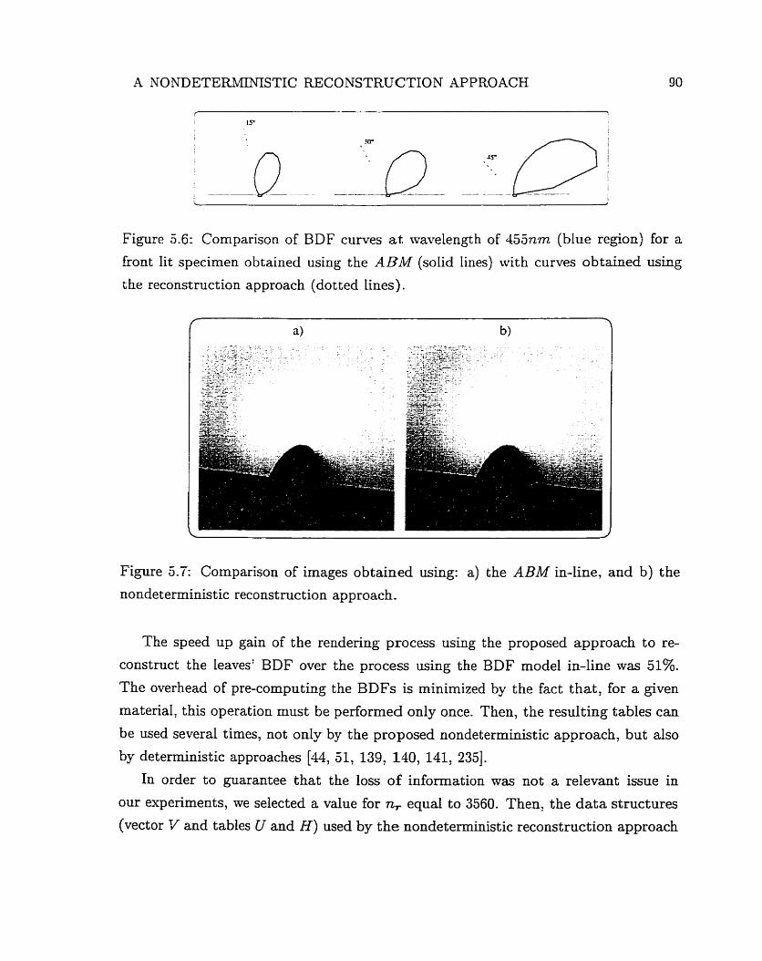
A NONDETERMINISTIC RECONSTRUCTION APPROACH
Figure 5.6: Cornparison of BDF curves at wavelength of 45572772 (blue region) for a
front lit specirnen obtained using the ABM (solid lines) with curves obtained using
the reconstruction approach (dot ted lines).
Figure 5.7: Cornparison of images obtained using: a) the ABM in-line, and b) the
nondeterministic reconstruction approach-
The speed up gain of the rendering process using the proposed approach to re-
construct the leaves' BDF over the process using the BDF mode1 in-line was 51%.
The overhead of pre-computing the BDFs is minimized by the fact that, for a given
material, this operation must be performed only once. Then, the resulting tables can
be used several times, not only by the proposed nondeterministic approach, but also
by deterministic approaches [44, 51, 139, 140, 141, 2351.
In order to guarantee that the loss of information was not a relevant issue in
our experiments, we selected a value for n, equal to 3560. Then, the da ta structures
(vector V and tables U and H) used by the nondeterministic reconstruction approach
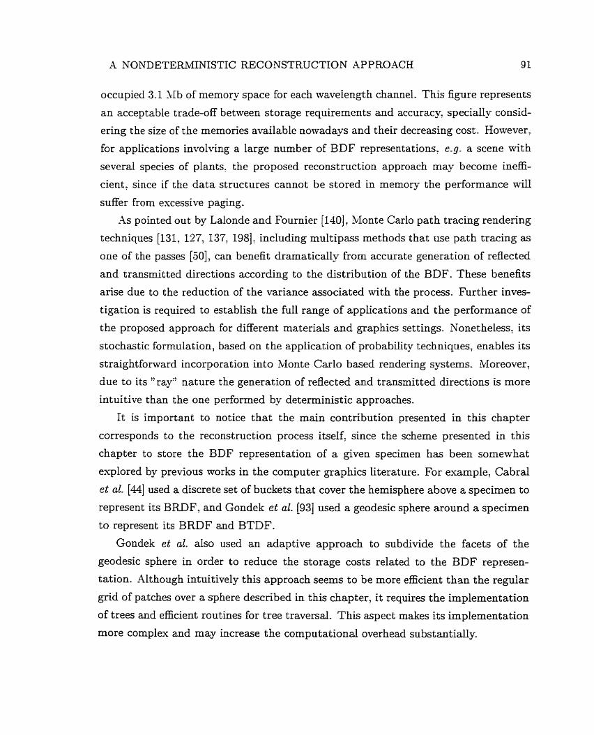
A NONDETERMINISTIC RECONSTRUCTION APPROACH 91
occupied 3-1 Mb of memory space for each wavelength channel. This figure represents
an acceptable trade-off between storage requirements and accuracy, specially consid-
ering the size of the memories available nowadays and their decreasing cost. However,
for applications involving a large number of BDF representations, e-g. a scene with
several species of plants, the proposed reconstruction approach rnay become ineffi-
cient, since if the data structures cannot be stored in mernory the performance Nil1
suffer from excessive paging.
-4s pointed out by Lalonde and Fournier [140], Monte Carlo path tracing rendering
techniques [131, 127, 137, 1981: including multipass methods that use path tracing as
one of the passes [SOI, can benefit dramatically from accurate generation of reflected
and transmitted directions according to the distribution of the BDF- These benefits
anse due to the reduction of the variance associated with the process. Further inves-
tigation is required to establish the full range of applications and the performance of
the proposed approach for different materials and graphics settings. Nonetheless, its
stochastic formulation, based on the application of probability techniques, enables its
straightfonvard incorporation into Monte Carlo based rendering systems. Moreover,
due to its '' ray" nature the generation of reflected and transrnitted directions is more
intuitive than the one performed by deterministic approaches.
It is important to notice that the main contribution presented in this chapter
corresponds to the reconstruction process itself, since the scheme presented in this
chapter to store the BDF representation of a given specimen has been somewhat
explored by previous works in the computer graphics literature. For example, Cabral
et al. [44] used a discrete set of buckets that cover the hemisphere above a specimen to
represent its BRDF, and Gondek et al. [93] used a geodesic sphere around a specimen
to represent its BRDF and BTDF.
Gondek et al. also used an adaptive approach to subdivide the facets of the
geodesic sphere in order to reduce the storage costs related to the BDF represen-
tation. Although intuitively this approach seems to be more efficient than the reguiar
grid of patches over a sphere descnbed in this chapter, it requires the implementation
of trees and efficient routines for tree traversal. This aspect makes its implementation
more cornplex and may increase the computational overhead substantially.
A NONDETERWSTIC RECONSTRUCTION APPROACH 92
Recall that during the pre-processing of the storage data structure, described
in Section 5.1.1. the patches that do not receive any hit are eliminated, implicitly
discarding elements of the grid that are not relevant for the BDF representation of a
given specimen. In other words, the storage scheme presented in this chapter. based
on a regular grid of patches, also allows an adaptive reduction of the memory costs
depending on the BDF representation a t hand.
un for tu na tel^., experimental data regarding performance and storage requirements
regarding the application of deterministic approaches is usually not readily available
in the literature. This aspect makes the cornparisons of the computational costs
involving the application of the proposed nondeterministic reconstruction approach
and the deterministic ones more difficult. -4 comprehensive assessrnent of their ad-
vantages and drawbacks would require a separate investigation, which, in turn, would
likely involve the implementation of the different reconstruction techniques and t heir
application to different test cases. We discuss this issue in more detail in Chapter 9.
5.4 Summary
We have presented a nondeterministic approach, based on standard Monte Carlo
techniques, for accessing arbitrary isotro pic reflect ance and transmittance functions.
The results obtained so far show that the reconstructed BDF curves present a high
degree of accuracy and the proposed reconstruction approach may provide a noticeable
gain in performance while keeping computational costs within reasonable limits.
As mentioned in Chapter 3, we might increase the accuracy of the spectral curves
provided by the ABU, e-g. b - adding features to account for masking and shadowing
effects. In this case the use of the reconstruction approach described in this chapter
could result in higher speed ups. But would the increase in image quality be suffi-
ciently noticeable to justify the increase on the model's complexity and the risk of
losing it dunng the reconstruction process? The answer to this question is not simple,
and involves the evaluation of several aspects related to the rendering process which
are beyond the scope of this thesis.
At this point of our research, instead of refining the ABM and relying solely on
reconstruction approaches to minimize its computational overheads, we decided to

A NONDETERi'MINISTIC RECONSTRUCTION APPROACH 93
follow a different path through the deveiopment of an alternative model. In this
alternative rnodel? presented in the next chapter. the processes of light interaction
with foliar tissues are simplified to a level in which the quality of the images is not
significantly affected, and the gains in performance are sufficiently high to justi- the
reduction in accuracy

A Simplified Mode1 for Light Interaction with Plant Tissue
The accuracy of simulations of light interaction with plants depends on the reflectance
and transmittance models for foliar tissues. The use of physically-based models is im-
portant for ensuring that rendering methods used in these simulations do not violate
the laws of ph-sics [146]. Moreover: these models have to be biologically-based in
order to appropriately account for the natural processes involved in these simula-
tions. Simplicity is also an important requirement for a reflectance model, since, as
pointed out by Ward [233], a model may otherwise become computationally irnprac-
tical. Thus, it is necessary to design practical reflectance and transmittance models
that a l h v us to render these materials fast nithout undermining the image quality.
In this chapter we present a simplified mode1 for light interaction u i th plant
tissue, which aims to provide a balance between two seerningly conflicting goals,
namely accuracy and efficiency. This model accounts for the three components of
plant tissues' BDF (surface reflectance, subsurface reflectance and transmittance),
and uses pre-cornputed reflectances and trammittances as scale factors in a stochastic
simulation of the scattering profile of these tissues. The use of these scale factors
replaces the time consuming random malk process used by the ABM to simulate the
randomization and the absorption of light within the foliar tissues. Moreover, this
approach reduces the number of rays needed to achieve a desired accuracy level in
the results.
These scale factors are computed off-line using the ABM. since the spectral curves
provided by this model have already been compared mith experimental data of real
foliar specimens, showing a good agreement (Section 4.6). Although the proposed
simplified model is oriented to leaves, like the ABM it can easily be extended to
A SIMPLIFIED MODEL FOR LIGHT INTERACTION WTTH PLANT TISSUE 95
other plant surfaces like petals and stems. We compare the results obtained using
the proposed simplified model with results obt ained applying the A BM in-line.
The remainder of this chapter is organized as follows:
Section 6.1 presents the proposed simplified model for light interaction with
plant tissue.
Section 6.2 provides an overview of aspects related to the implementation of the
simplified mode1 and a summary of its parameters.
Section 6.3 describes the testing parameters and procedures.
Section 6.4 examines the testing results, focusing on cornparisons n i th the A BM.
Finally, Section 6.5 closes t his chapter with a summary of the main character-
istics of the proposed simplified model.
6.1 The Simplified Mode1
In the simplified model light propagation is also described in terms of rajr optics,
and the interaction of light with the foliar tissues is described in terms of their SPF
(Section 2.2). As pointed out by Glassner 1861, the BDF (or, in this case, the SPF) is a
difficult function to work with due to its dependence on several variables. Fortunately,
we can make some simplifjmg assumptions about the foliar tissues that give us a more
computationally convenient expression to manipulate.
First, we assume that the physical properties describing the light propagation
are identical everywhere within the foliar tissues, i.e. they can be considered as ho-
mogeneous interacting media [96]. This assumption allows us to leave out the po-
sitional argument. Second, since the anisotropy of plant leaves is considered to be
associated with their venation system (Section 3.2), and considering that the biolog-
ical data regarding these systems is scarce to support the design of a biologically-
based anisotropic reflectance model for these materials, we also assume that they
are isotropic. This assumption allows us to work with only one parameter for the
incidence direction qi, which is given by the angle of incidence, Bi, of an incident ray
tMth respect to the normal of a leaf-
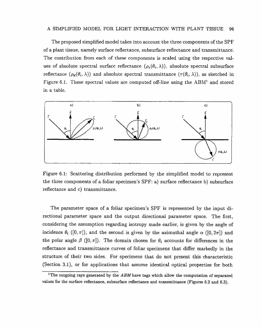
A SMPLIFIED MODEL FOR LIGHT INTERACTION WITH PLANT TISSUE 96
The proposed simplified model takes into account the three components of the SPF
of a plant tissue, namely surface reflectance: subsurface reflectance and transmit tance.
The contribution h m each of these components is scaled using the respective val-
ues of absolute spectral surface reflectance (p , (Bi , A ) ) , absolute spectral subsurface
reflectance (pd(Bi A ) ) and absolute spectral transmittance (r(& A ) ) as sketched in
Figure 6.1. These spectral values are computed off-line using the ABM1 and stored
in a table.
Figure 6.1: Scattering distribution perforrned by the simplified model to represent
the three components of a foliar specimen's SPF: a) surface reflectance b) subsurface
reflectance and c) transmit tance.
The parameter space of a foliar specimen's SPF is represented by the input di-
rectional parameter space and the output directional parameter space. The first,
considering the assumption regarding isotropy made earlier, is given by the angle of
incidence Bi ([O, TI), and the second is given by the azimuthal angle rr ([O, Zn]) and
the polar angle 13 ([O, n]). The domain chosen for Oi accounts for differences in the
reflectance and transmittance curves of foliar specimens that differ markediy in the
structure of their two sides. For specimens that do not present this characteristic
(Section 3 4 , or for applications that assume identical optical properties for both
The outgouig rays generated by the A BM have tags which d o w the computatian of separated
values for the surface reflectance: subsurface reflectance and transmittance (Figures 6.2 and 6.3).
A SIMPLIFTED MODEL FOR LIGHT INTERACTION W T H PLANT TISSUE 97
sides [135], the domain of Bi can be narrowed to [O. $1. - Initially, to account for the surface component of a foliar specimen's SPF for a
given incident ray, Rie obtain the corresponding reflected ray using the lam of reflection
(Section 2.1). Then. to simulate the effects of the epidermal cells' shape on the
reflected rays at the air-+epidemal cells interface, nre perturb the refiected rays using
a warping function (Equation 4.1) based on an exponentiated cosine distribution
(Appendiu A) employed by the ABM
-4s mentioned earlier, mhen light passes to the interna1 foliar tissues its direction
of travel is randomized and it becomes diffuse. This randomization of the incident
rays results in a near-Lambertian distribution for the subsurface reflectance of a fo-
liar specimen, and a near-Lambertian distribution for its transmittance. In order to
simulate the distribution of rays regarding these two components, tve perturb the nor-
mai of the foliar specimen instead of the incident ray- The orientation of the normal
used in the perturbation depends on the incidence g e o m e t - If the incident ray hits
the foliar specimen's front (adaxial epidermis) we use the normal for the subsurface
reflectance component and its opposite vector for the transmittance component. O th-
envise, ive use the normal and its opposite vector the other way around. For these
perturbations me use a warping function (Equatioo 4.2) based on a cosine distribution
(Appendiu A), also employed by the ABM.
6.2 Implementation Overview and Summary of Parameters
The simplified model was also implemented Cf+ in order to take advantage of
the object oriented features of this programming language. This model, like the
ABM, can be incorporated as a self-contained class in a graphics Library, such as the
ggLibrary [202], and be used by different global rendering methods.
Since the values for spectral reflectance and transmittance are pre-computed, the
set of model parameters is reduced to the oblateness of the epidermal cells, ob, used in
the perturbations of the reflected rays, and the angle of incidence, Bi, used to access
the table of absolute spectral reflectances and transmittances. The angle of incidence
is computed using Equation 5.1.
A SIMPLIFIED MODEL FOR LIGHT INTERACTION WITH PLANT TISSUE 98
The images presented in Section 6.4 were generated using a modified version of
Kajiya's path tracing [131, 1981. For the computation of the direct light contribution
ive selected the scale factors pd(Bi, A) and T(&, A ) according to the position of the
light source mith respect to the foliar specimen. This selection was made using the
angle of the shadow ray with respect to the specirnen's normal' 8,: and applying the
"B,,X) if 00 < 8, 5 900 K
- for light corning from below 90" < 8, < 180"
if 90° < Bi < lSOO A
tFfhile the ABM uses an elcplicit mechanism to simulate the absorption of light,
the simplified model relies on the absorption probabilities implicitly associated with
the scaling factors. In order to perform fair cornparisons between these two mod-
els (Section 6.4): we use an adaptive tree-depth control [104] based on cumulative
ray attenuation (attenuation, for short) in our implementation of the modified path
tracing algorithm. In this context the attenuation of a given ray is obtained through
the product of reflectances and/or transmittances of the surfaces which are hit in the
rafs path [198].
During rendering this attenuation is compared with a cutoff attenuation threshold,
qc, to control the depth of the tree during the ray tracing. If the attenuation is smdler
than cc, the ray's path is terminated. For a given scene we select a value for c, to limit
the maximum depth of both trees (one associated with the process using the simpiified
model aod the other with the process using the ABM) to the same percentage of rays
to be propagated (0.01%). We examine this issue in more detail in the next section.
Since the attenuation has three values corresponding to the three RGB channels, we
convert it to luminance in order to compare it 6 t h a selected cc. This conversion is
A SIMPLIFIED MODEL FOR LIGHT INTERACTION W T H PLANT TISSUE 99
made using the folloning SLIPTE formula [148]:
6.3 Testing Issues
For our experiments me selected foliar data regarding a soybean leaf (Section 4.5.2).
The spectral measurements needed to compute the table of absolute spectral re-
flectances and transmittances were made using a virtual spectrophotometer (Sec-
tion 4-51) and 106 rays in regular intervals of 1" for the angIe of incidence Bi ([O, x]).
The comparisons regarding the foliar specimen's BDF presented in the ne- section
were performed using a virtual goniophotometer (Section 4.5.1) with a collecter sphere
divided into 20 patches along its latitude and 40 patches along its longitude, and using
108 rays to generate each BDF curve associated with a given wavelength.
For the reasons presented in the previous chapter, we sarnpled the absorption
spectra of chlorophyll (Figure 4.4) in the dominant wavelengt hs corresponding to
SMPTE monitor chromaticity coordinates (Table 5.1). Shen, applying the ABM.
we compute the table of absolute spectral reflectances and transmittances used to
generate the curves and images presented in the next section. Figure 6.2 presents the
graphs correspondings to the entries of t his table.
The table of absolute spectral reflectances and transmittances for the veins, as
described in the previous chapter, also obtained using the ABM and the SMPTE
monitor chromaticity coordinates, but with the absorption spectra of chlorophyll (Fig-
ure 4.4) scaled by a factor of 0.1 according to biological data provided by McClendon
and Fukshansky [lST]. Figure 6.3 presents the graphs corresponding to the entries of
this table.
We used the geometrical descriptions of soybean leaves presented in Section 5.2
to generate the images presented in the next section. For a given graphics setting the
measurements regarding both models were performed on the same machine. More-
over, the models were implemented using the same software guidelines to avoid dif-
ferences that could affect the timing. The root-mean-square (RMS) errors [86] of
the difference images, presented in the next section, were computed from normalized
pixel values (scaled to [O, 11) , and using Equation 6.2.

A SIMPLIFIED ,MODEL FOR LIGHT INTERACTION WITH PLANT TISSUE 100
T
Red (b608nm) - Front Lit t
Green (A755 hm) - Front Lit
- - Red (k608nm) - Back Lit
Green ( M 5 1 nm) - Back Lit
0 2
9.1
angle of incidence (Hi )
Blue ( k 4 5 5 n m ) - Front Lit
- 1
1 - - - - 8
- as,
O- . <
o ~ o z o m 1 ~ w m ; o m ~ d angle of incidence (8i)
Blue (k455nrn) - Back Lit
a7
angle of incidence (8i) - /
Figure 6.2: Graphs corresponding to the entries of the table of absolute spectral
reflectances and transmittances for a soybean leaf.
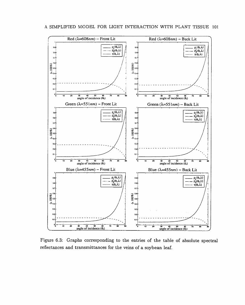
A SIMPLIFIED MODEL FOR LIGHT INTERACTION WITH PLANT TISSUE
r
Red (k=608nm) - Front Lit Red (As608nm) - Back Lit
Green ( k 5 5 lnm) - Front Lit
angle of incidence (8i)
BIue ( M 5 5 n m ) - Front Lit
01 O I C 2 0 Y J U ) M ü O M 6 0
ringle of incidence (Bi)
Green ( k 5 5 Inm) - Back Lit
o.2t - - - - - - - - - - - - - - - - - - - - - - y-. f
Blue ( M 5 5 n r n ) - Back Lit 1 l
0.9 - 18-
0
angle of incidence (8;) mgle of incidence (8i) J
Figure 6.3: Graphs corresponding to the entries of the table of absolute spectral
reflectances and transmittances for the veins of a soybean leaf.
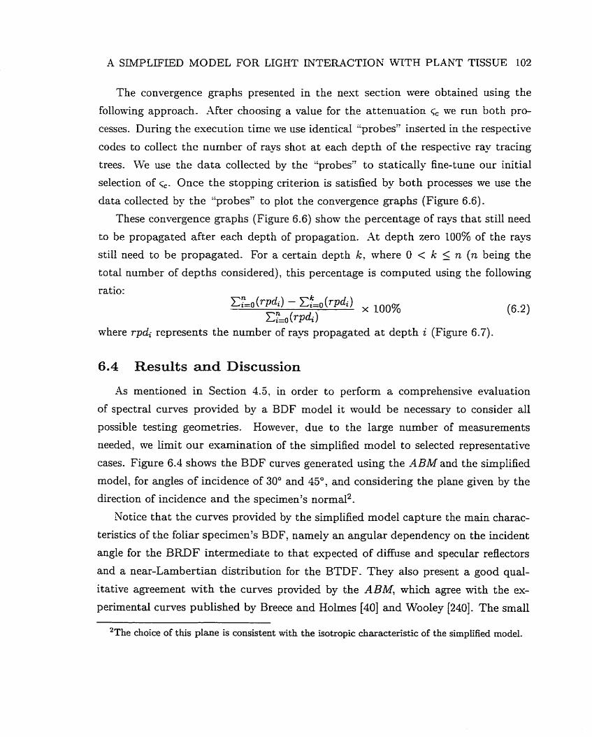
A SIMPLIFIED MODEL FOR LIGHT IIL'TERACTION WTTH PLANT TISSUE 102
The convergence graphs presented in the next section were obtained using the
following approach. -Ifter choosing a value for the attenuation G we run both pro-
cesses. During the execution time we use identical "probes" inserted in the respective
codes to collect the number of rays shot at each depth of the respective ray tracing
trees. We use the data collected by the "probes" to statically fine-tune our initial
selection of c,. Once the stopping criterion is satisfied by both processes we use the
data collected by the "probes" to plot the convergence graphs (Figure 6.6).
These convergence graphs (Figure 6.6) show the percentage of rays that still need
to be propagated after each depth of propagation. At depth zero 100% of the rays
still need to be propagated. For a certain depth k: where O < k 5 ri (n being the
total number of depths considered), this percentage is computed using the following
ratio:
where rpdi represents the number of rays propagated a t depth i (Figure 6.7).
6.4 Results and Discussion
As mentioned in Section 4.5, in order to perform a comprehensive evaluation
of spectral curves provided by a BDF model it would be necessary to consider al1
possible testing geometries. However, due to the large number of measurernents
needed, ive limit our examination of the simplified model to selected representative
cases. Figure 6.4 shows the BDF curves generated using the ABM and the simplified
model, for angles of incidence of 30" and & O , and considering the plane given by the
direction of incidence and the specimen's normal2.
Notice that the curves provided by the simplified model capture the main charac-
teristics of the foliar specimen's BDF, namely an angular dependency on the incident
angle for the BRDF intermediate to that expected of diffuse and specular reflectors
and a near-Lambertian distribution for the BTDF. They also present a good qual-
itative agreement M t h the curves provided by the ABM, which agree with the ex-
perimental curves published by Breece and Holmes [40] and Wooley [240]. The small
2The choice of this plane is consistent with the isotropic characteristic of the simplified model.
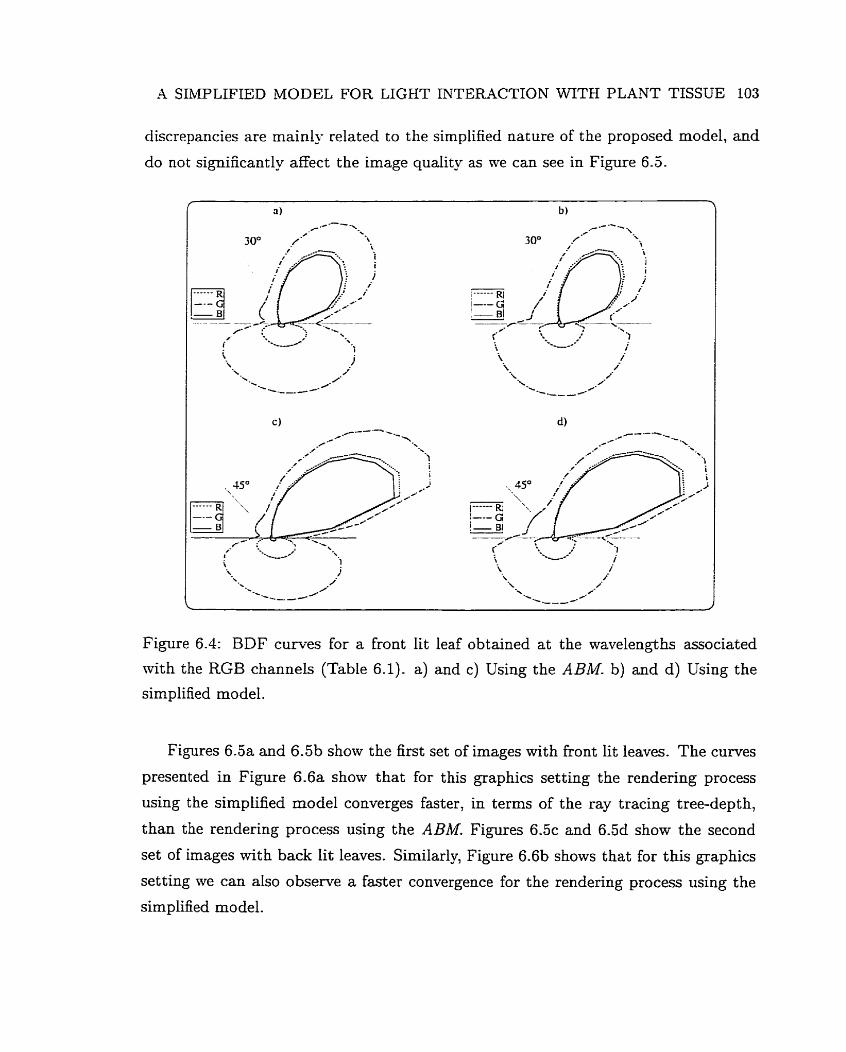
A SIMPLIFLED MODEL FOR LIGHT INTERACTION WITH PLANT TISSUE 103
discrepancies are mainly related to the simplified nature of the proposed model, and
do not significantly affect the image quality as we can see in Figure 6.3.
Figure 6.4: BDF curves for a front lit leaf obtained at the wavelengths associated
with the RGB channels (Table 6.1). a) and c) Using the ABM. b) and d) Using the
simplified model.
Figures 6.5a and 6.5b show the first set of images with front lit leaves. The curves
presented in Figure 6.6a show that for this graphics setting the rendering process
using the simplified mode1 converges faster, in terms of the ray tracing tree-depth,
than the rendering process using the ABM. Figures 6 . 5 ~ and 6.5d show the second
set of images with back lit leaves. Similarly, Figure 6.6b shows that for this graphics
setting me can also observe a faster convergence for the rendering process using the
simplified model.
A SIMPLIFIED MODEL FOR LIGHT GL'TERACTION WITH PLANT TISSUE 104
Figure 6.5: Top row: Bont lit leaves (1"' set) using the ABM (a) and the simplified
mode1 (b). Middle row: back lit leaves (2nd set) using the ABM (c) and the simplified
model (d). Bottom row: Images with ambient light only (3rd set) and using the ABM
(e) and the simplified model (f). For al1 three scenes we used G = 0.01.
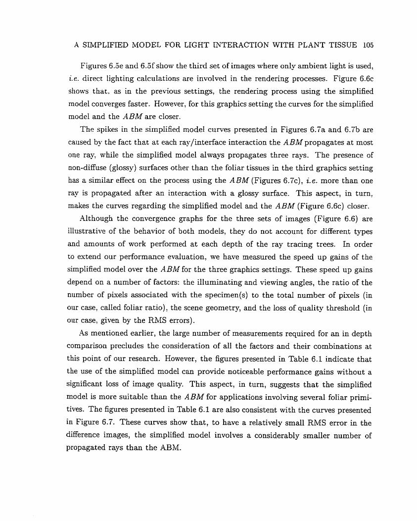
A SIMPLIFIED MODEL FOR LIGHT INTERACTION W T H PLANT TISSUE 105
Figures 6.5e and 6.5f show the t hird set of images mhere only ambient light is used,
ie. direct lighting calculations are involved in the rendering processes. Figure 6 . 6 ~
shows that. as in the previous settings: the rendering process using the simplified
rnodel converges faster. However, for this graphics setting the curves for the simplified
rnodel and the il BM are closer.
The spikes in the simplified model curves presented in Figures 6.Ïa and 6.7b are
caused by- the fact that at each raylinterface interaction the ABM propagates at most
one ray: while the simplified model always propagates three rays. The presence of
non-diffuse (glossy) surfaces ot her t han the foliar tissues in the t hird graphics set ting
has a similar effect on the process using the ABM (Figures 6 . 7 ~ ) ~ i. e. more than one
ray is propagated after an interaction with a glossy surface. This aspect, in turn,
rnakes the curves regarding the simplified model and the ABM (Figure 6 .6~ ) closer.
Although the convergence graphs for the three sets of images (Figure 6.6) are
illustrative of the behavior of both models, they do not account for different types
and amounts of work performed a t each depth of the ray tracing trees. In order
to estend Our performance evaluation, we have rneasured the speed up gains of the
simplified mode1 over the ABM for the three graphics settings. These speed up gains
depend on a number of factors: the illurninating and viewing angles, the ratio of the
number of pixels associated wïth the specimen(s) to the total number of pixels (in
our case, called foliar ratio), the scene geometry, and the loss of quality threshold (in
our case, given by the RMS errors).
-4s mentioned earlier, the large number of measurements required for an in depth
cornparison predudes the consideration of al1 the factors and their combinations at
this point of Our research. However, the figures presented in Table 6.1 indicate that
the use of the simplified model can provide noticeable performance gains without a
significant loss of image quality. This aspect, in turn, suggests that the sirnplified
model is more suitable than the ABM for applications involving several foliar primi-
tives. The figures presented in Table 6.1 are also consistent wïth the curves presented
in Figure 6.7. These curves show that, to have a relatively small RMS error in the
difference images, the simplified mode1 involves a considerably smaller number of
propagated rays than the ABM.
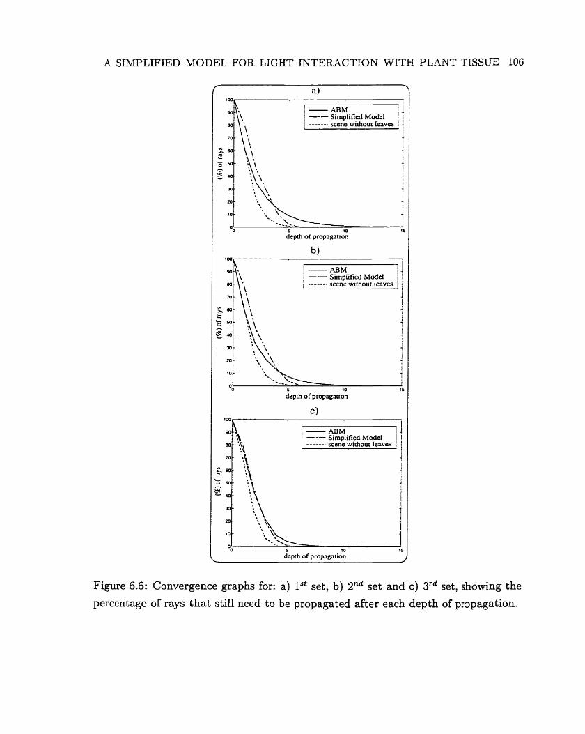
A SIMPLIFBD AUODEL FOR LIGHT INTERACTION WITH PLALVT TISSUE 106
depth of propagation
6 )
depth of propagauon
cl
depth of propagation d
Figure 6.6: Convergence graphs for: a) lSt set, b) 2nd set and c) 3rd set, showing the
percentage of rays that still need to be propagated after each depth of propagation.
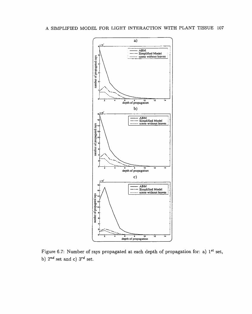
A SIMPLIFTED MODEL FOR LIGHT INTERACTION WTTH PLANT TISSUE 107
l a r . .IO'
1
I 7
1
I
1 0 12 14
depth of propagation J
6 8 1 0 12 14
depth of propagation
Simplified Mode1 scenr without l a v e s
depth of propagation
Sirnplified Model scene without leaves I
Figure 6.7: Number of rays propagated at each depth of propagation for: a) 1'' set,
b) 2"d set and c) 3rd set.
A SIklPLIFED MODEL FOR LIGHT INTERACTION WITH PLANT TISSUE 108
--- - - -
Image set foliar ratio RMS error speed up
Red Green Blue
Table 6.1: Comparison of accuracy us. performance gain.
In order to reduce noise in the images due to Monte Car10 path tracing integration,
ive used a large number of sample points per pixel, which increased the absolute
time measurements. For instance, the image presented in Figure 6.5f was generated
using 400 sarnp!e points per pkel and it took 93 minutes (elapsed CPU time) on a
SGI R10000. The incorporation of the mode1 into more efficient global illumination
frameworks may considerably reduce the overall rendering time.
The overhead of pre-computing the table of reflectances and transmittances is
reduced by the fact that, for a given foliar specimen, thiç operation rnust be per-
forrned only once. Shen, the resulting table can be used several times not only in the
rendering of individual leaves, but also in global illumination calculations involving
vegetation canopies [155]. Furthermore, the table look-ups are performed through
direct indexing, and its storage requirements are wïthin reasonable Iimits. For in-
stance, the table used in our testing experiments requires only 14.5 Kb of storage
space. Even if finer sampling resolutions are used in the measurement of reflectances
and transmittances, we believe that the use of such a table provides a worthwhile
trade-off between accuracy and computational costs, specially consideriog the sizes
of the mernories available nowadays and their decreasing costs.
The quality of images of organic materials is affected by several factors beyond
the scope of this dissertation. Certainly, the use of more realistic geometric models
would improve the realism of these images. However, it is important to notice that
despite the sophisticated geometrical models of foliar tissues available in the graphics
literature [32, 69, 106, 108, 180], to the best of our knomledge there is still a lack of
geometrical models that accurately account for their venation system as well.
Bump mapping [30] c m be used to reduce this problem, by perturbing the normal
A SIMPLIFIED ,MODEL FOR LIGHT INTERACTION WTH PLANT TISSUE 109
of the surface to simulate a wrinkle or a vein. However, as pointed out by Glassner
[86], it precludes the simulation of phenomena such as the self-blocking and self-
shadowing of incident light by the veins, since it does not alter the geometry of the
surface. Displacement mapping [6O] : a technique t hat actually alters the geomet ry of
the surface, allows the simulation of these phenomena. but, as pointed out by Watt
and Watt L23.11: it presents the drawback of being difficult to incorporate in a standard
polygonal mesh renderer.
The use of accurate furninaire data, including its geometrical description, po-
sitional information, and spatial and spectral intensity information [lO4], can also
improve the quality of these images significantly. Moreover, since the rendering of
organic materials Like plants have a strong wavelength dependency, the use of more
efficient methods for guiding the wavelength selection, such as the strategy proposed
by Meyer [160], as well as an investigation to determine the group of wavelengths
that fits best the perceptual requirements of these applications could also improve
the overall quality of the images of these materials.
6.5 Summary
In t his chapter we have presented a physically and biologically-based model for
light interaction with plant tissue that can be incorporated into rendering systems
without a significant computational overhead. -4lthough: as mentioned in Chapter 4,
the evaluation of a computer model is less predictable than measuring physical phe-
nomena, our esperiments suggest that despite of its simplified nature, the proposed
model captures the general behavior of foliar BDFs and does not introduce significant
errors along the rendering pipeline. Moreover, the low storage requirements and the
signficant speed ups provided by the simplified mode1 make it more suitable than the
ABM for applications involving sewral foliar primitives. Alt hough the scale factors
used by the simplified model were computed using the ABM, their computation can
be performed through more accurate BDF models as they become available.
Like the ABM, the simplified model can be extended to incorporate anisotropic
characteristics of the foliar tissues. The current limited knowledge about these char-
acteristics, however, h a . driven us to treat these matenals as isotropic. In fact we
A STMPLIFIED MODEL FOR LIGHT INTERACTION WITH PLANT TISSUE 110
have exploited the assumption of isotropy of foliar specimens' BDF to cornpress the
reflectance and transmittance data. Although the isotropy assumption may seem
restrictive, it is relevant to notice that techniques have been proposed in the com-
puter graphics literature [67] to transform a tabulated anisotropic BDF to match the
isotropy property in order to reduce storage and cornputational costs in r ende~ng
applications. Incidentalllv, transformation techniques based on single value decompo-
sition ( S V ' ) type approaches [92] can also be used to make a BDF separable [67].
-1s appropriately mentioned by Fournier [1T] and DeYoung and Fournier [67], trans-
forniing a BDF to be separable alloms radiosity computations (Chapters 7 and 8) to
be performed more efficiently for surfaces whose BDFs present complex directional
charact erist ics [l6ï].
We have also outlined in this chapter some aspects beyond the scope of this
dissertation that can contribute to the realism of images of plants. -4mong these
aspects are the spectral sampling and the geometrîcal representation of veins. Another
important aspect related to the quality of these images is the global illumination
framework through which they are generated. This aspect bnngs back the trade-off
between accuracy and efficiency. By proposing plausible BDF models for plants we
have contributed to the improvement of the overall accuracy of global illumination
applications involving these materials. In the nest chapters we intend to present our
contributions regarding the efficiency of global illumination applications associated
with radiosity with faster iterative solutions for radiosity systems.
Eigen-Analysis for Radiosity Systems
Determining the radiance of each surface of a closed environment using the radiosity
rnethod demands the solution of a linear system of equations. This system represents
the balance of energy in the environment. Because of the large size of the linear sys-
tems associated with radiosity applications and the relatively low accuracies required
in the solutions (only 1% to IO%, since humans do not perceive finer variations of
light [l7O]) , iterative methods are commonly used.
In this chapter we first describe the radiosity system of linear equations and present
some selected iterative methods usually applied to solve these systems. Then, we use
this mathematical background to examine the spectral properties of these systems
which affect the performance of the iterative methods directly. More specifically, we
look a t the spectrum or set of eigenvalues of the radiosity coefficient mat* and its
relationship to the convergence of the iterative methods.
Furt hermore, Rie show analytically t hat al1 the eigenvalues of the radiosity coeffi-
cient rnatrix are real and positive. Mthough one could in theory apply any iterative
method to solve the radiosity system of linear equations, this fact enables the appli-
cation of fast methods, such as the Chebyshev method (described iii Chapter 8), with
confidence of their convergence.
We focus the discussion presented in this chapter on standard, or classical [86],
radiosity applications involving diffuse BRDFs. The insights drawn from our analysis,
however; are also valid for applications involving materials that present BDFs with
Lambertian and non-lambertian characteristics and handled by multipass methods
that use the radiosity method in one of the passes [50: 168, 2311.
The sections of this chapter are organized as follows:
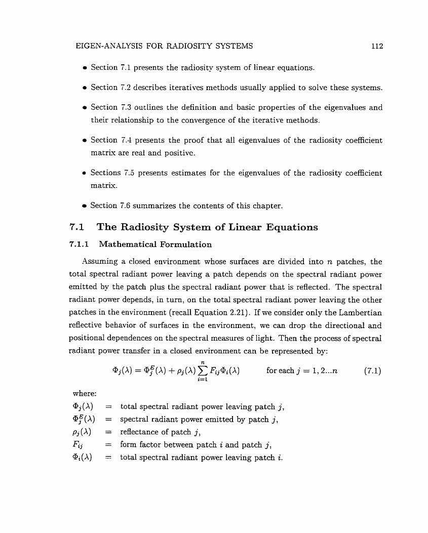
EIGEN-ANALYSE FOR FMDIOSITY SYSTEMS
Section 7.1 presents the radiosity system of linear equations.
Section 7.2 describes iteratives methods usually applied to solve these systems.
Section 7.3 out lines the definition and basic properties of the eigenvalues and
t heir relationship to the convergence of the iterative methods.
Section 7.4 presents the proof that al1 eigenvalues of the radiosity coefficient
rnatrix are real and positive.
e Sections 7.5 presents estimates for the eigenvalues of the radiosity coefficient
mat Ku.
Section 7.6 summarizes the contents of this chapter.
7.1 The Radiosity System of Linear Equations
7.1.1 Mathematical Formulation
Assuming a closed environment whose surfaces are divided into n patches, the
total spectral radiant power leaving a patch depends on the spectral radiant power
emitted by the patch plus the spectral radiant power that is reflected. The spectral
radiant power depends, in turn, on the total spectral radiant power leaving the other
patches in the environment (recall Equation 2.21). If we consider only the Lambertian
reflective behavior of surfaces in the environment, we c m drop the directional and
positional dependences on the spectral measures of light. Shen the process of spectral
radiant power transfer in a closed environment can be represented by:
where:
Gj(X) = total spectral radiant power leaving patch j ,
Q>iE(A) = spectral radiant power emitted by patch j,
p j (X ) = reflectance of patch j ,
Fij = form factor between patch i and patch j, = total spectral radiant power leaving patch i.
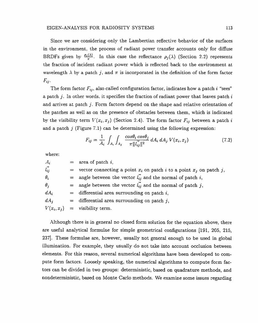
EIGEN-hVALYSIS FOR RADIOSITY SYSTEMS 113
Since we are considering only the Lambertian reflective behavior of the surfaces
in the environment, the process of radiant power transfer accounts only for diffuse
BRDFs given b - 9. In this case the refiectance pj(X) (Section 2.2) represents
the fraction of incident radiant power which is reflected back to the environment at
waveIength X by a patch j , and 71- is incorporated in the definition of the form factor
Fij-
The form factor Fijo also called configuration factor, indicates how a patch i "sees"
a patch j. In other words. it specifies the fraction of radiant power that leaves patch i
and arrives at patch j. Form factors depend on the shape and relative orientation of
the patches as well as on the presence of obstacIes between thern, which is indicated
by the visibility term ['(xi: xj) (Section 2.4). The form factor Fi, between a patch i
and a patch j (Figure 7.1) can be determined using the foilowing expression:
where:
area of patch i:
vector connecting a point Xi on patch î to a point xj on patch j,
angle between the vector 1, and the normal of patch i,
angle between the vector 1, and the normal of patch j7
differential area surrounding on patch i,
differential area surrounding on patch j ,
visibility term.
Although there is in general no closed form solution for the equation above, there
are useful analytical formulae for simple geometrical configurations [N 1, 205, 2 15,
2371. These formulae are: however, usually not general enough to be used in global
illumination. For example, they usually do not take into account occlusion bettveen
elements. For this reason, several numerical algorithms have been developed to com-
pute form factors. Loosely speaking, the numerical algorithms to compute form fac-
tors can be divided in two groups: deterrninistic, based on quadrature methods, and
nondeterministic, based on Monte Carlo methods. We examine some issues regarding
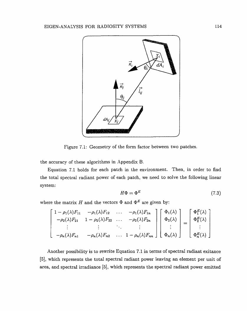
EIGEN-ANALYSIS FOR EUDIOSITY SYSTEMS
Figure 7.1: Geometry of the form factor between two patches.
the accuracy of these algorithms in Appendix B.
Equation 7.1 holds for each patch in the environment. Then, in order to find
the total spectral radiant power of each patch? we need to solve the following linear
system:
H@ = a E (7.3)
where the mat rk H and the vectors and < P E are given by:
Another possibility is to rewrite Equation 7.1 in terms of spectral radiant exitance
[5], which represents the total spectral radiant power leaving an element per unit of
area, and spectral irradiance [5], which represents the spectral radiant power emitted
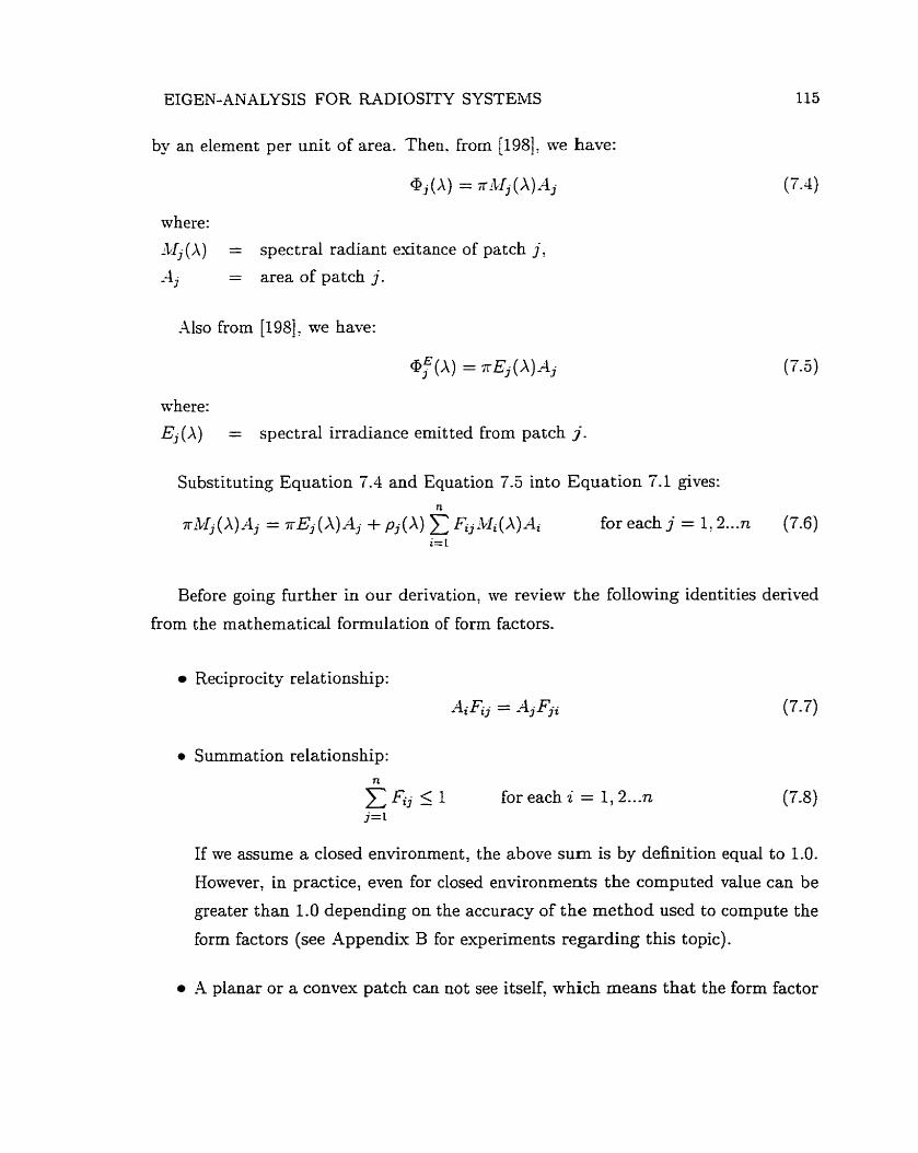
EIGEN-ANALYSIS FOR RADIOSITY SYSTEMS
by an element per unit of area. Then. from [198]: we have:
where:
;bfj(j(X) = spectral radiant exitance of patch j .
= area of patch j.
Also from [198]. we have:
where:
Ej (A) = spectral irradiance emitted from patch j .
Substituting Equation 7.4 and Equation 7.5 into Equation 7.1 gives: n
~ i l l j (A).+ = TE, (X)Aj + pj (A) C F,iWi ( A ) A i for each j = 1,2 ... n (7.6) i= 1
Before going further in our derivation, ive review the following identities derived
from the mathematical formulation of form factors.
Reciprocity relationship:
-&Fij = -4-F.- 3 32
0 Summation relationship: n
X E ~ S ~ for each i = 1,2 ... n ('7.8) j=l
If ive assume a closed environment, the above sum is by definition equal to 1.0.
However, in practice, even for closed environments the computed value can be
greater than 1.0 depending on the accuracy of the method used to compute the
form factors (see -4ppendix B for experiments regarding this topic) .
A planar or a convex patch can not see itself, which means that the form factor
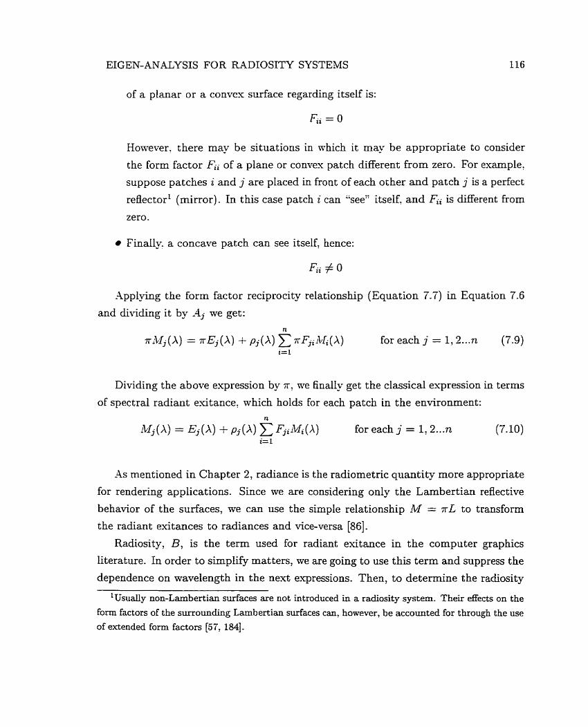
EIGEN-ANALYSIS FOR RADIOSLTY SYSTEMS
of a planar or a convex surface regarding itself is:
Homevert there may be situations in which it may be appropriate to consider
the form factor Fii of a plane or convex patch different from zero. For example:
suppose patches i and j are placed in front of each other and patch j is a perfect
re£lectorL (mirror) . In this case patch i can Pee" itself, and Fii is different from
zero.
Final13 a concave patch can see itself, hence:
Applying the form factor reciprocity relationship (Equation 7.7) in Equation 7.6
and dividing it by iIj we get: IL
r i L f j (A) = xEj (A) + pj (A) C 5qiATi(X) for each j = 1,2 ... n (7.9) i= 1
Dividing the above expression by ir; we final- get the classical expression in terms
of spectral radiant exitance, which holds for each patch in the environment: n
i"r, (A) = Ej (A) + pj (A) C F,ihfi(A) for each j = 1: 2 . ~ 2 (7.10) i= 1
As mentioned in Chapter 2, radiance is the radiometric quantity more appropriate
for rendering applications. Since we are considering only the Lambertian reflective
behavior of the surfaces, we can use the simple relationship M = TL to transform
the radiant exitances to radiances and vice-versa [86].
Radiosity, B, is the term used for radiant exitance in the cornputer graphics
literature. In order to simpli% matters, we are going to use this term and suppress the
dependence on wavelength in the next expressions. Then, to determine the radiosity
'Usually non-Larnbertian surfaces are not introduced in a radiosity system. Their effects on the
form factors of the surrounding Lambertian surfaces can, however, be accounted for through the use
of extended f o m factors [57, 1841.
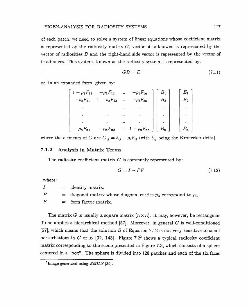
EIGEN-ANALYSE FOR RADIOSITY SYSTEMS 117
of each patcli. ive need to solve a system of linear equations whose coefficient rnatrk'r
is represented by the radiosity matrix G! vector of u n h m is represented by the
vector of radiosities B and the right-hand side vector is represented by the vector of
irradiances. This system, known as the radiosity system. is represented by:
ort in an espanded form, given by:
where the elements of G are Gij = 6, - piFij (with bij being the Kronecker delta).
7.1.2 Andysis in Matrix Terms
The radiosity coefficient rnatrix G is commonly represented by:
where:
I = identity mat rk ,
P = diagonal matrix whose diagonal entries pii correspond to pi,
F = form factor mat rk .
The matrk G is usually a square mat rk (n x n). It may, however, be rectangular
if one applies a hierarchical method [57]. Moreover, in general G is well-conditioned
[57], which means that the solution B of Equation 7.12 is not very sensitive to small
perturbations in G or E [92, 1431. Figure 7.22 shows a typical radiosity coefficient
m a t e corresponding to the scene presented in Figure 7.3, which consists of a sphere
centered in a "box". The sphere is divided into 128 patches and each of the six faces
'Image generated usîng EMILY [39].
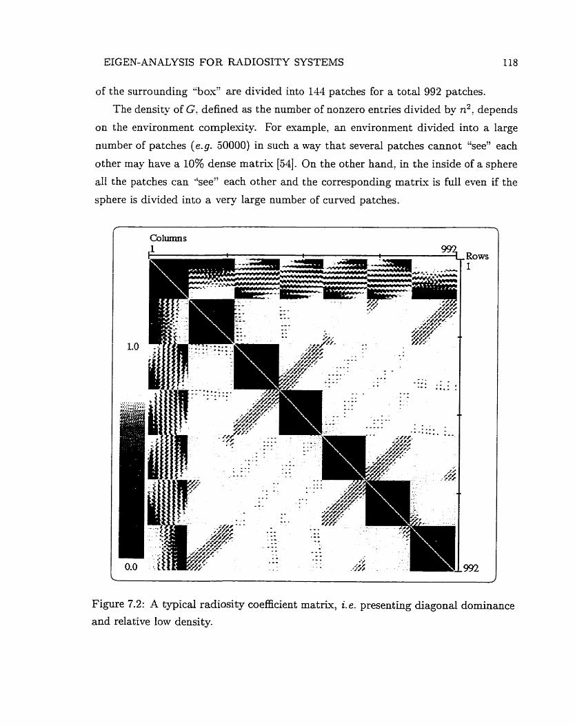
EIGEN-ANALYSIS FOR RADIOSITY SYSTEMS
of the surrounding *box" are divided into 144 patches for a total 992 patches.
The density of Gy defined as the number of nonzero entries divided by n2; depends
on the environment cornplexit- For example, an environment divided into a large
number of patches (e-g. 50000) in such a way that several patches cannot "see" each
other may have a 10% dense matrix [54]. On the other hand, in the inside of a sphere
a11 the patches can "sec" each other and the corresponding matrix is full even if the
sphere is divided into a very large number of curved patches.
. Rows 1
Figure 7.2: A typical radiosity coefficient matrix, i. e. presenting diagonal dominance
and relative low density.
EIGEN-ANALYSIS FOR RADIOSITY SYSTEMS
Figure 7.3: An image generated using the radiosity method.
Notice that the density depends more Qn the placement of patches in the environ-
ment than on the number of patches. For euample, by changing the level of occlusion
in the scene present in Figure 7.3 (e.g. by changing the radius of the sphere) we can
increase the number of zero entries, represented by the black areas in Figure 7.2, and,
in turn, reduce the density of the matrïu. A matrix entry is equal to zero when:
Fij = O for i # j (due to occlusion or patches placed in the same plane);
p = O (black patches, which does not occur in real environments, although
sometimes researchers assign p = O to light sources).
EIGEN-ANALYSIS FOR RADIOSITY SYSTEMS 120
Assuming that O 5 p < 1 and that the sum of form factors in any row is equal to
one, w-e can say that the matrix G is strictly diagonally dominant, since the following
property (also noticeable in Figure 7.2):
holds for each j = 1: 2, - - - , n- However, if ive inchde, for experimental purposes: a perfect reflector surface3
(pi = 1 ) in the environment: we cannot ensure dominance of rows. In this case, weak
diagonal dominance [243] holds, chat is 1 Gii ( 2 Cjn,,,i+j lGij 1, unless al1 pi = 1.
7.2 Solutions for Radiosity Systems
Why should we search for &ter methods to solve the radiosity system of equations
when the most expensive stage of the radiosity pipeline (in some cases up to 90% of
the cornputational time [242]) is the caIculation of form factors? The reason is that
there are many practical applications in which a radiosity system has ta be solved
repeatedly, due to changes either to the vector of reftectances or to the vector of
irradiances, while the forrn factors remain unchanged.
Examples of such applications would be sun and shade simulations for environ-
mental design purposes (Figure 7.4) or the simulation of solar radiation over a forest
canopy for remote sensing purposes. For a comprehensive sun and shade simulation
corresponding to a period of twelve hours, the form factors would have to be com-
puted only once, while the system would have to be solved 720 times to account for
solar positions at every minute.
Direct methods for solving linear systems, such as Gaussian Elimination [42] or
LU decomposition [42], are not suitable for large radiosity systems of equations be-
cause of the relative low density of the coefficient matrix, and because rapid solutions
at relatively low accuracy are needed. These aspects plus the special properties of
3A perfect reflector surface is a plane surface reflecting ail the incident light in a perfect image-
fonning state, such that we cannot focus on the surface. In other words, there is no visible microstruc-
ture, and visually there is no surface at d [128]. Thus, we cannot have pi = 1 in any physically
realistic system [57]. Nevertheless such a surface can be useful as a gloss standard [122, 1281.
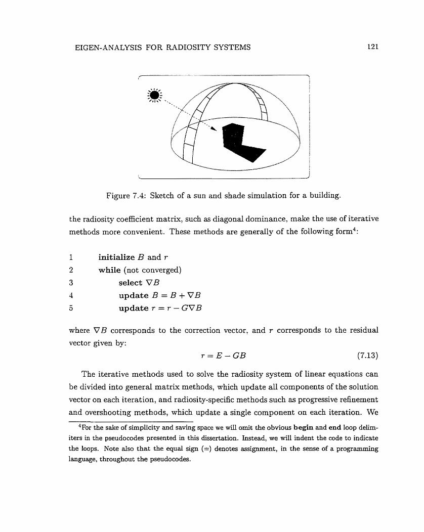
EIGEN-ANALYSIS FOR RADIOSI'IY SYSTEMS
Figure 7.4: Sketch of a sun and shade simulation for a building.
the radiosity coefficient matriu, such as diagonal dominance, make the use of iterative
meth~ds more convenient. These methods are generdly of the follovving form4:
i initialize B and r
2 while (not converged)
3 select VB
4 update B = B + V B - a update r = r - GVB
where V B corresponds to the correction vector, and T corresponds to the residual
vector given by:
T E E - G B (7.13)
The iterative methods used to solve the radiosity system of linear equations can
be divided into general matrix methods, which update al1 components of the solution
vector on each iteration, and radiosity-specific methods such as progressive refinement
and overshooting methods, which update a single component on each iteration. We
'For the sake of simplicity and saving space we will omit the obvious begin and end loop delim-
iters in the pseudocodes presented in this dissertation. Instead, we will indent the code to îndicate
the loops. Note also that the equal sign (=) denotes assignment, in the sense of a programming
language, t hroughout the pseudocodes.
EIGEN-ANALYSIS FOR R4DIOSITY SYSTEMS 122
use the expression radiosit y-specific methods to group met hods specifically developed
to solve the radiosity problem. Although those methods can be considered variations
of numerical methods such as Southwell Iteration [91] or SOR (Section 72.2); they
have been adjusted and fine-tuned to the radiosity case.
7.2.1 The Gauss-Seidel Method
An example of a general m a t r ~ ~ method is the Gauss-Seidel method [21? 1011,
which was introduced to solve the radiosity system of Linear equations by Cohen and
Greenberg [55]. This rnethod adapted to the radiosity contert becomes the following:
1 for (al1 z )
2 Bi = starting guess
3 while (not converged)
4 for i = 1 ,2 , ..., n
5 Bi = Ei -F Pi Cy=,,jpi(BjFi,) 6 display image using Bi as the radiosity of the patch i.
Usually the vector of irradiances is used as the starting guess. This algorithm
estimates the radiosity of a patch i by adding its irradiance, and au the radiosity that
it reflects @ne 5). It uses the most recent estimates of the radiosities of d l patches
to estimate the radiosity of patch i. The physical interpretation consists of gathering
the radiosity from other patches to estimate the incoming radiosity. It converges
quiclcly due to the diagonal dominance of the radiosity coefficient matrix. After a
few passes through the rnatrix we get the final image. Gauss-Seidel can have 0(n2)
memory requirement if the matrix G is dense and its elements are stored. There
are applications (see Chapter 8), however, for which the benefits of having G stored
overcome the memory costs.
7.2.2 The Successive Overrelaxation Method
The Successive Overrelaxation method (SOR) [21] consists of applying extrapo-
lation to the Gauss-Seidel method. This extrapolation takes the fo r a of a weighted
average between the previous iterate and the computed Gauss-Seidel iterate, for
EIGEN-ANALYSIS FOR RAD1C)SITY SYSTEMS 133
each component. The physical interpretation is that instead of gathering the cor-
rect amount of r ad ios i t~ an extrapolation factor w is used to take into account steps
that will occur later on in the process.
The structure of the SOR algorithm is similar to that of the Gauss-Seidel algo-
rithm. If ur = 1.0 then the SOR Method becomes the Gauss-Seidel Method. Its algo-
rithnï can be obtained by replacing line 3 of the algorithm presented in Section 7.2.1
by: n
The major difficulty of this method is to choose the best value of w which gives the
fast est convergence. This factor depends on the problem characteristics. However, the
idea of overrelaxation is exploited in the context of progressive refinement methods,
and it can be thought of as overshooting (Section 7.2.4).
7.2.3 The Progressive Refinement Method
The progressive refinement approach [54], which was later shown to be equivalent
to Southwel17s relaxation method [90: 911, allows us to obtain intermediate images
and to reduce the storage requirement to O ( n ) by computing the form factors on the
for (al1 i)
VBi = O
ABi = Eï
while (not converged)
select i' S U C ~ that ABiAi is largest
VBi = VBi + ABi
for every other patch j
Arad = pjFji4Bi
ABj = ABj + Arad
ABi = O
display intermediate image using ABk + V B k as the radiosity of patch k.
EIGEN-ANALYSIS FOR RADIOSITY SYSTEbIS 124
In the previous algorithm Ai represents the area of patch i, ilBi represents the
amount of "unshot" radiosity and VBi represents the amount of %hot'7 radiosity
(VBi = Bi - ABi). More formally ABi represents the residual r: and VBi represents
the vector of unknowns that we are solving for. During one iteration, the patch with
t.he largest "energy" to shoot: i. e. largest ABi-+: is chosen and its radiosity is shot
through the environment. So, in this caseo the physical interpretation consists of
shooting instead of gathering process. -As a result the other patches may receive some
new radiosity Arad. The intermediate images obtained in the early steps tend to be
dim, so an ambient term is added [54]. As the iteration process goes on this ambient
term is reduced until the final image is obtained. The ambient term is a weighted
sum of the unshot radiosities of al1 patches in the entironment:
where Ai corresponds to the area of patch i and R corresponds to the overall inter-
reflection factor R, which is given by: 1
where p,, corresponds to an average reflectance for the environment [54], which can
be computed as an area-weighted average of the patch reflectances such that:
7.2.4 The Overshooting Approach
In the original progressive refinement approach
(7.16)
a patch may need to shoot ra-
diosity multiple times. Overshooting algorithms based on overrelaxation have been
introduced to solve this problem [73, 90, 194, 2431. One such an algorithm was pro-
posed by Feda and Purgathofer [73]. The main idea behind these algorithms consists
of shooting the current radiosity of the patch plus an estimate that accounts for ra-
diosity that will return due to the reflection by other patches. This approach can
reduce the overall number of iterations required. Feda and Purgathofer use the ambi-
ent term not only for display purposes, but also as the overshooting arnount. As was
mentioned earlier, several methods have been proposed to implernent overshooting.
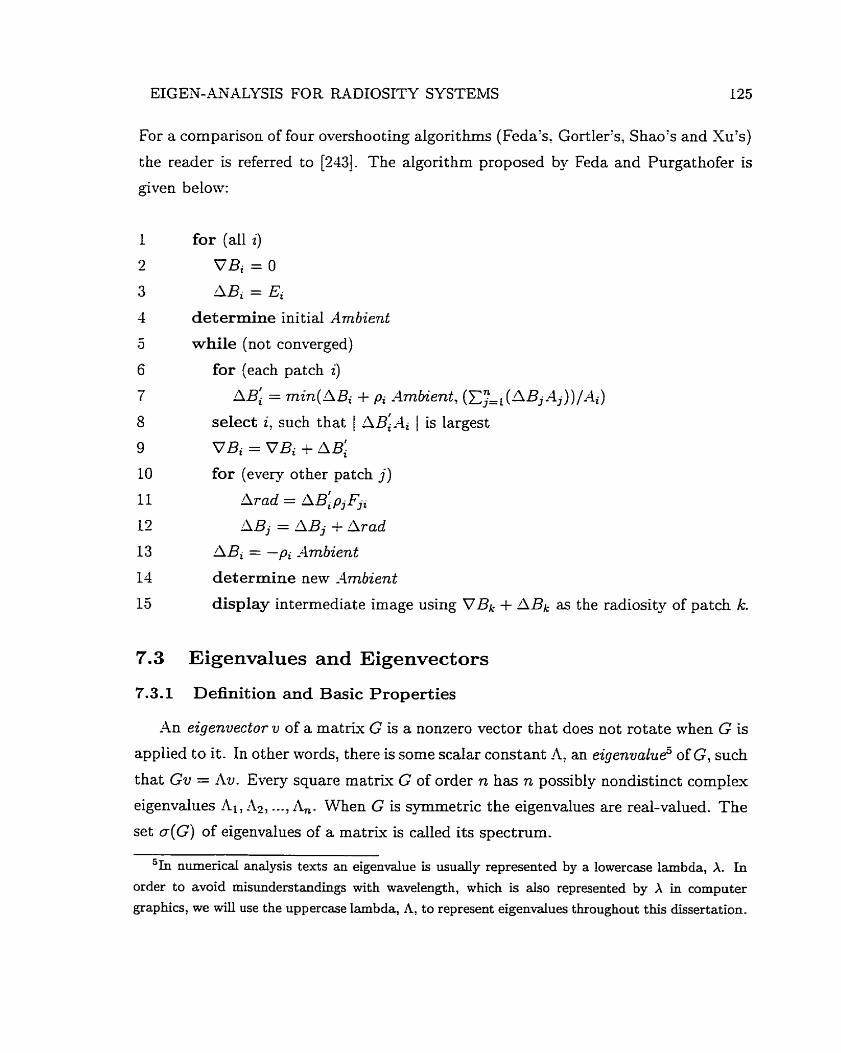
EIGEK-AXUYSIS FOR RADIOSITY SYSTEMS 125
For a cornparison of four overshooting algorithm (Feda's, Gortler's, Shao's and Xu's)
the reader is referred to [2431. The algorithm proposed by Feda and Purgathofer is
given below:
for (al1 i)
VBi = O
AB, = Ei
determine initial ilrnbient
while (not converged)
for (each patch z )
AB: = mmin(ABi + pi Ambient, (C:=, (4BjAj))/ili)
select i, such that 1 1 1 ~ : ~ ~ 1 is Largest
VBï = VBi + AB:
for (every other patch j )
Arad = A B : ~ ~ F , ~
ABj = AB, + Arad
ABi = -pi Arnbient
determine new Ambient
display intermediate image using VBk + ABk as the radiosity of patch k.
Eigenvalues and Eigenvectors
Definition and Basic Properties
An eigenvector v of a matrix G is a nonzero vector that does not rotate when G is
applied to it. In other words, there is some scalar constant A, an eigenualue5 of G, such
that Gu = Au. Every square matrïx G of order n has n possibly nondistinct complex
eigenvalues Ai, A2, - --, A,. When G is symmetric the eigenvalues are real-valued. The
set a(G) of eigenvalues of a matrix is called its spectrum.
51n numerical analysis texts an eigenvalue is usually represented by a lowercase lambda, A. In
order to avaid misunderstandings with wavelength, which is also represented by X in computer
graphies, we will use the uppercase lambda, A, to represent eigenvaiues throughout this dissertation.
EIGEN-ANALYSIS FOR RADIOSITY SYSTEMS 126
In order to find the eigenvalues of a square n x n rnatrix like G, we may resort to
concepts from the t heory of determinants [lG], such as the characteristic polynomial
of G given by:
p(h) = det (G - -11) (7.17)
The zeros of p ( A ) represent the eigenvahes or characteristic values of the m a t r k
G. If there is a vector u # O such that (G - I l ) u = O holds, then u represents
an eigenvector or characteristic vector of G corresponding to the eigenvalue A. This
eigenvector is only determined up to a scalar multiple.
7.3.2 Relationship with Iterative Methods
The eigenvalues of certain matrices determine the convergence of iterative methods
used to solve the radiosity system GB = E. For linear stationary methods of the
where k is the number of iterations made, which includes Gauss-Seidel and SOR, the
eigenvalues of the iteration matrix T are the relevant ones. The matrix T is derived
from the coefficient matris G. For example, in the Gauss-Seidel iteration, T is given
by :
T = ( D + L)-'u (7.19)
where:
D = diagonal part of G,
L = strictly Iower triangular part of G, U = strictly upper triangular part of G.
There needs to be no connection between the eigenvalues of T and those of G.
Linear stationary methods converge if e(T) < 1, where Q(T) is the spectral radius of
T6. Furthemore, convergence is faster for smaller e(T).
6The spectral radius e ( K ) of a matrix K is defined by e(K) = rnax 1 A [, where A is an eigenvalue
of K [42]- The spectral radius is usuaily represented in numericd analysis te.xt by p, but, to avoid
misunderstanding with the reflectance, also represented by p, we are going to represent it by g
throughout this dissertation.
EIGEWANALYSIS FOR RADIOSITY SYSTEMS
For nonstationary methods such as Conjugate Gradient or Chebyshev (Chapter 8),
the eigenvalues of the coefficient matriv G are the important ones. The Chebyshev
method has convergence deterrnined by the radius of the convex hull of the spectrum
of G. which is determined by the estreme eigenvalues. For a m a t r k with positive
real eigenvalues. which is the case of G (see proof presented in the next section); the
largest ( I ) and smallest (A,,,) eigenvalues cornpletely determine convergence,
which: as d e s c ~ b e d by Hageman and Young [101]: is faster for larger values of the
following ratio:
The convergence of the Conjugate Gradient method is determined by the overall
distribution of eigenvalues, and even for a given a (G) it is impossible to predict
the exact number of iterations that this method wil1 require. However, Conjugate
Gradient generally requires only k + 1 iterations when the eigenvalues occur in only
k < n cl us ter^^ and has façter convergence for larger values of the ratio presented
above (Equation 7.20). We examine this issue in more detail in Section 8.2.3.
7.4 Proof that Al1 Eigenvalues of the Radiosity Coefficient
Matrix are Real and Positive
Given a n x n matrix G, the n x n m a t r k obtained by interchanging the r o m and
columns of G is called the transpose of G and is denoted by Gt [143]. In other terms,
Gt- - = Go. A square rnatrix G is said to be symmetric if G = Gf. The radiosity 3 = coefficient matrix is not syrnmetric; however, if it is multiplied by a diagonal m a t r k
Q, where the diagonal entry Q, represents the quotient of the area and the reaectance
of patch i, then the resulting m a t r ~ ~ :
is symmetric.
Since QG is symmetric, its eigenvalues are real-valued. Moreover, by applying the
Gerschgorin Circle Theorem (Section 7 4 , one can ver ie that they are also positive
EIGEN-ANALYSE FOR RADIOSITY SYSTEMS 128
(see the eigenvalue estimates of G" presented in the next section). Hence, QG is a
positive definite ma t rk by Theorem 9.12 of Burden and Faires [42] which states:
A symmetric rnatrix -4 is positive definite if and only if al1 the eigenvalues
of -4 are positive.
The definition of positive definite means that :
for al1 x E Cn7 where C is the complex plane and xH is the conjugate transpose of the
column vector x.
Let x be an eigenvector of G and il be an eigenvalue. Shen:
where A and x f O are possibly complex.
Then:
QGx = hQx (7.24)
and
The left side of Equation (7.25) is necessarily real and positive from Equation (7.22).
Furthermore, the definition of an eigenvector x implies that it is nonzero, hence:
where
&min = min Qii
Since al1 Qii > O, Equations (7.25) and (7.26) imply that h is real and A > 0.
Therefore, al1 of the eigenvalues of G are real and positive.
Arvo [7, 91 has shown that several fundamental operators that arise in global
illumination c m be uniformly approximated by matrices. Although it may seem that
this proof applies directly to the continuous radiosity operator, more details need to
EIGEN-ANALYSIS FOR RADIOSITY SYSTEMS 129
be considered. The critical point is that the diagonal entry i of the mat ri^ Q is the
ratio of the area and reflectance of the i-th patch.
For the continuous case. the area is zero and the above argument cannot be used
direct- However, the continuous operator is a compact operator [9]' sometimes ais0
called a completely continuous operator in functional analysis. Because of this: me
can construct a sequence of finite dimensional operators Gk that converge uniformly
to the continuous operator G,, each with a spectrum consisting only of positive
real eigenvalues. That sequence can be constructed using a sequence of uniformly
refined discretizations of the scene, for example. The limit G, will necessarily have
a spectrum that is real and nonnegative. Because G, is nonsingular7 [131], it cannot
have zero as an eigenvalue. Its compactness also implies that it has only a point
spectrum, which implies that G, has only positive real eigenvalues in i ts spectrum.
7.5 Eigenvalues Estimates for Radiosity Applications
As discussed earlier (Section 7.3-2): the convergence properties of iterative solvers
rely extensively on the set of eigenvalues of the corresponding coefficient matrku. It
was also noted (Section 7.3.1) that the eigenvalues of G can be obtained, in theory,
by finding the roots of its characteristic polynomial. In practice, as pointed out
by Burden and Faires [@], i t is difficult to determine the roots of an nth-degree
polpomial except for small values of n. Then, approximation techniques, such as the
Power method [41, 421, Lanczos algorithm [64, 921 or QR Factorization [41, 421, are
commonly used to compute the eigenvalues.
Usually to calculate the eigenvalues of a m a t e G through these techniques re-
quires more computation than that required to solve the corresponding linear system.
However, ive can obtain relatively inexpensive estimates of the eigenvalues using the
Gerschgorin Circle Theorem [41]. This theorem says that the eigenvalues of G are
contained nrithin the union of n circles Si, which have center Gii and radius x:j;i lGijl
7An n x n rnatRx K is said to be nonsingdar if an n x n rnatrix K-1 (the inverse of K) k s t s
such that KK-L = K-'K = I [42]. -2lternatively a matrix K is also said to be nonsingular if its
determinant is nonzero [143].
EIGEN-ANALYSIS FOR RADIOSITY SYSTEMS
and are defined by: n
j#ï
where C is the cornplex plane. The union of any k of these circles that do not
intersect the remaining (n - k) must contain precisely k (counting multiplicities) of
the eigenvalues.
In the case of the radiosity matriv G? if we assume an environment formed by
planar or convex surfaces (Fii = O) then al1 the main diagonal entries ni11 be equal
to 1.0- So the centers of the circles are also equal to 1.0. In addition, if we assume a
closed environment (xy=, Fij = 1), then the radius is given by pi. In practice, if the
numerical method used to compute the form factors does not provide exact results
(Appendix B). then the radius is in fact given by pi(l & 6); where 6 corresponds to
the numerical error associated with the summation of form factors of patch i.
Neumann [165] and recently Nievergelt [169] have applied the Gerschgorin Circle
Theorem to obtain estirnates for the eigenvalues of the symmetric ma t rk Gs. Due
its symmetry, GS has onIy real eigenvalues. Shen, instead of circles in the plane
of complex numbers. we only have to deal with real intervals. The proof that all
eigenvalues of the nonsymmetric radiosity matrix G are real and positive, presented
in the previous section: allows us to apply the Gerschgorin Circle Theorem in the
same manner to G. In other words, we need to consider only real intervals, instead
of circles in the plane of complex numbers, to estimate the largest and the smallest
eigenvdues of G. One can use these estimates to apply the Chebyshev method to the
solution of radiosity system. We discuss this issue in more detail in the next chapter.
7.6 Summary
The average radiosity (or radiant exitance) of n patches of a closed environment
can be approlumated by solving a Iinear system with n unknowns. When n is srnall
(ie. less than few thousands of patches), general mat& methods like Gauss-Seidel
can be used where the explicit .n x n ma t rk can be pre-computed and stored [55].
When n is large, progressive techniques are used where the matrix rows or elements
are recomputed as needed [54]. When n is very large (ie. hundreds of thousands of
EIGEN-ANALYSE FOR RADIOSITY SYSTEMS 131
patches). stochastic techniques can avoid computing or storing the n2 elements of the
matrk [166].
In applications where n is srnall enough to store the encire m a t r k in main memol ,
general m a t r k techniques mil1 be faster than progressive techniques8. For euample,
for Sun and shade simulations [99] the lighting can be esamined on simple geometric
approximations of the environment being designed. and n can be very srnall. When
the color scheme and lighting are being designed, the computationally expensive part
(form factors) of the r n a t r i ~ in the linear system can be reused as the matenal prop-
erties are changed. For these applications the fastest possible general matrïx solution
is desirable.
In this chapter we have outlined important characteristics of the linear systems
arising in radiosity applications and described iterative methods usually applied to
solve theses systems. 310reover~ we have proved that al1 eigenvalues of the radiosity
coefficient matris area real positive. This fact is essential for the application of faster
iterative solvers to the radiosity systerns such as the Chebyshev met hod [2lï].
The concepts presented in this chapter Ml1 be built upon in the following chapter
to est end our investigation on the spectral characteristics of the radiosity systems
and their effects on the convergence of the iterative methods. In addition, we are
going to present two nonstationary methods? namely the Conjugate Gradient [118,
1951 (previously examined in the graphics literature by Heckbert [117; 1151) and
the Chebyshev [217] methods. We espect that these non-stationary methods may
outperform the stationary and radiosity-specific methods previously described, which
is borne out by the cornpanson results presented in the next chapter.
'Progressive techniques will initially converge faster because they can begin iterations before
cornputing the entire matriu. If general matrix techniques are modified to gradually constmct the
matrk during initial iterations, then this advantage of progressive method goes away.
CHAPTER 8
Searching for Fast Solutions for Radiosity Systems
As we mentioned in the previous chapter. radiosity-specific methods (Sections 7.2.3
and 7.2.4) used to solve the radiosity system allow us to have a rough preview of the
overall illumination of a scene after few steps of iteration. However, as mentioned
y Cohen et al. [Ml: since few patches contribute to the overall illumination in the
early stages of the iterative process (unless the iteration is started v e v close to the
solution), detailed illumination effects, such as color bleeding, are lost. Radiosity-
specific methods have to iterate until the desired convergence is reached to avoid that
loss. This rneans that, even though they do not need to store al1 the form factors,
radiosity-specific methods still have to compute al1 of them, possibly ma- times.
Suppose we want to generate severai similar images to produce a computer mi-
mated sequence. Since there is some significant coherence from frame to frarne, we do
not need to preview al1 the frames. The first images can be used as a preview of the
whole sequence. For these applications nre would like to generate the images in the
shortest possible time, i.e. to solve the radiosity linear systems as fast as possible. In
this chapter we are going to show that general matrïx methods (Section 7.2) can be
faster than methods that converge in a smaller nurnber of steps of iteration, namely
the radiosi-specific met hods l .
Usually the form factors are computed on the fly when one uses a radiosity-
specific method. The same approach can be applied if one uses a general matrix
method. However, by storing the form factors we have the additional advantage
of avoiding the cost of recomputing them repeatedly. In fact, several applications
'For this discussion we assume a conventional EUSC architecture, where coherent memory access
is vital.
SEARCHING FOR FAST SOLUTIONS FOR RADIOSITY SYSTEMS 133
present characteristics that make the off-line computation and storage of the form
factors more convenient t han t heir computation on demand:
Simulations involvïng Light ing and/or reflect ance changes do not require new
form factor cornputations in order to solve the radiosity system. Under these
circumstances the only restriction to store the form factor mat rk may be its
size if a given application involves a large nurnber of primitives and/or finer
meshes. For these applications one can use techniques, such as hierarchical
radiosity [HO: 111: 2061 and clustering [208. 209: 2161, to reduce the the form
factors storage costs. Although the order of the radiosity matrix associated
nrith these applications is usually high; the nonzero entries are mostly located
in diagonal blocks that can be stored without a significant memory cost and
solved in parallel.
Scene subdivision techniques, such as those used by the FIAT [78] and Lucifer
approaches [76? 1451, can be used to separate a large equation system into a col-
lection of small subsystems. For esample, recently Shinya et al. [196] proposed
a modified hierarchical algorithm using virtual walls, which regards a large ra-
diosity system as a collection of small subsystems. The subsystems interact
with others only through input and output functions. Since the data necessary
for each subsystem computation is completely localized, the database can be
stored on disk. Shinya et al. daim that their algorithm c m work in time corn-
plesity O(n) for scenes divided into n subsystems, while classical hierarchical
radiosity algori t hms run with O (n2) cornplexity
The view-independent radiosity solution regarding the first pass of a multipass-
method usually requires the tessellation of the environment in a coarse mesh
[198], since view-dependent passes are going to be applied later to handle the
high frequency signals. For these coarse meshes the dimensions of the corre-
sponding radiosity matrices are fairly small, and they can be stored without a
significant memory cost .
For applications in which only small geometrical changes are made, acceleration
techniques [22, 49, 831 can be used to speed the process of recomputing the

SE-4RCHING FOR FAST SOLUTIONS FOR MDIOSITY SYSTEMS 134
form factors. For example, if the geometry of a scene changes from one frarne
to another in the computer a~imat ion application mentioned earlier, only a
small fraction of the form factors need to be recomputed due to the animation
coherence. In this case most of the fonn factors can be precomputed in an
off-line operation and stored. The remaining ones can be recomputed, without
a significant overhead. using the techniques cited above.
For environments with high average reflectance and high level of occlusion, which
occur very often in architectural and remote sensing applications [48], the iteration
process takes a longer time to converge due to the characteristics of the radiosity
m a t r k For example, mhen the overall reflectance of an environment approaches 1.0,
the spectral radius of the iteration matrix (for a stationary method like Gauss-Seidel)
also approaches 1.0, and the linear solvers converge slowly. In this chapter ive test
the performance of a nonstationary general ma t rk method, the Conjugate Gradient
method [1l8], and introduce another nonstationary general rnatrk method, namely
the Chebyshev rnethod [217]. which can converge faster than any other iterative
method mentioned in the graphics literature to date in those situations.
The remaining of this chapter is organized as follows:
Section 8.1 discusses mathematical tools used to analyze most iterative solvers
for linear systems.
Section 8.2 presents the Conjugate Gradient method.
Section 8.3 outlines the main properties of the Chebyshev polynomids.
Section 8.4 introduces the Chebyshev method.
Section 8.5 describes the parameters and procedures used in our investigation
of fast er solutions for radiosity systems.
Section 8.6 examines the convergence of the iterative methods in small amounts
of time, as opposed to a small number of iterations, and the effects of reflectance
and occlusion changes on the performance of these methods.
FinaUy, Section 8.7 summarizes the contents this chapter.
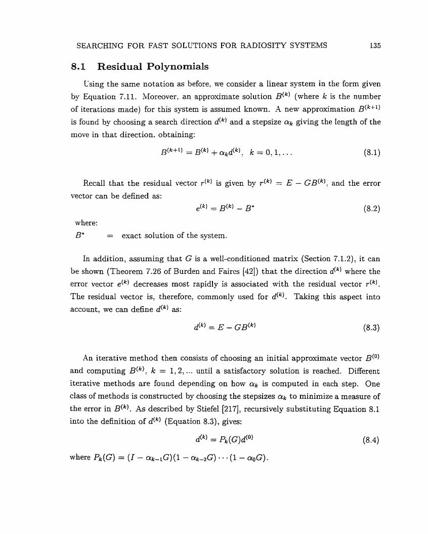
SEARCHING FOR FAST SOLUTIONS FOR R4DIOSITY SYSTEMS 135
8.1 Residual Polynomials
Using the same notation as before, we consider a Iinear çystern in the form given
b Equation 7-11. Moreover. an approximate solution B(") (where k is the number
of iterations made) for this system is assumed known. -4 new approximation B(~+')
is found by choosing a search direction d(k) and a stepsize a,, giving the length of the
move in that direction. obtaining:
B("+~) = B ( ~ ) f ~ u ~ d ( ~ ) ' k = O , 1, . . .
Recall that the residual vector r(') is given by dk) = E
vector can be defined as: = ~ ( k ) - B*
where:
B* = exact solution of the system.
GB(k) . and the error
(8-2)
In addition, assuming that G is a well-conditioned matrLu (Section 7.1.2): it can
be shown (Theorem 7.26 of Burden and Faires [42]) that the direction d(k) where the
error vector e(k) decreases most rapidly is associated with the residual vector dk). The residual vector is. therefore, commonly used for d("). Taking this aspect into
account, we can define d(k) as:
&) = E - G B ( ~ ) (8-3)
An iterative method then consists of choosing an initial approximate vector B(')
and computing ~ ( " 1 , k = 1,2, ... until a satisfactory solution is reached. Different
iterative methods are found depending on how olk is computed in each step. One
class of methods is constructed by choosing the stepsizes a k to minimize a measure of
the error in ~ ( " 1 . As described by Stiefel [2 171, recursively substituting Equation 8.1
into the definition of d(k) (Equation 8.3), gives:
where Pk(G) = (1 - crk-lG)(l- ~ k - 2 G ) - - - (1 - ~ o G ) -
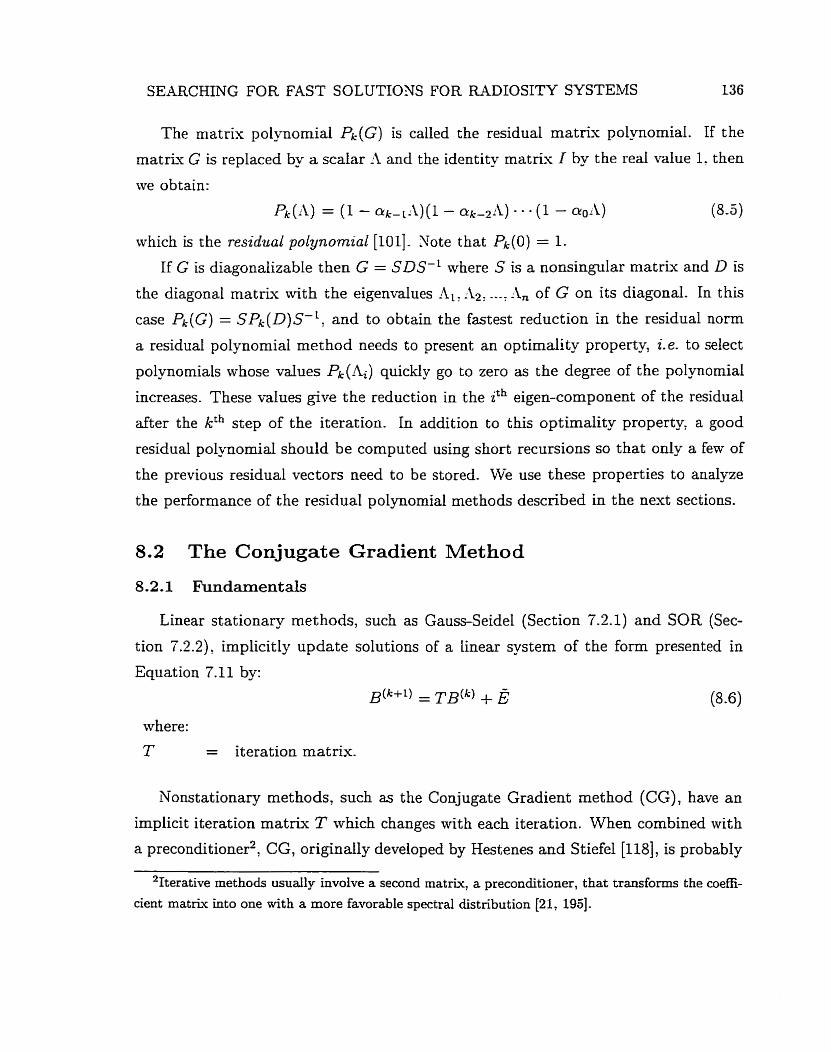
SEARCHING FOR FAST SOLUTIONS FOR RADIOSITY SYSTEMS 136
The ma t rk polynornial Pk(G) is called the residual rnatrk polynomial. If the
rnatriu G is replaced by a scalar il and the identity matriu I by the reai value 1. t hen
we obtain:
Pk(lI) = (1 - ak-L1I) (1 - ak-2ii) - - - (1 - a0LI) (8-5)
which is the residval polynornial [101]. Yote that Pk(0) = 1.
If G is diagonalizable then G = SDS-L where S is a nonsingular rnatrk and D is
the diagonal matrkv with the eigenwlues AL: ;12: ---: -L of G on its diagonal. In this
case Pk(G) = SPk(D)S-': and to obtain the fastest reduction in the residual n o m
a residual polynomial method needs to present an optimality property, ie. to select
polynornials whose values Pk(Ai) quickly go to zero as the degree of the polynomial
increases. Shese values give the reduction in the ith eigen-component of the residual
after the kth step of the iteration. In addition to this optimality property, a good
residual polynomial should be cornputed using short recursions so that only a few of
the previous residual vectors need to be stored. TVe use these properties to analyze
the performance of the residual polynomial methods described in the next sections.
8.2 The Conjugate Gradient Method
8.2.1 Fundarnent als
Linear stationary methods, such as Gauss-Seidel (Section 7.2.1) and SOR (Sec-
tion ï.2.2)? implicitly update solutions of a linear system of the form presented in
Equation 7.11 by: gW+" ) + É (8-6)
where :
T - - iteration matrLu.
Nonstationary methods, such as the Conjugate Gradient method (CG), have an
implicit iteration m a t e T which changes with each iteration. When combined with
a ~reconditioner*, CG, originally developed by Hestenes and Stiefel (1181, is probably
%erative methods usually involve a second matrix, a preconditioner, that transforms the coeffi-
cient matrkv into one with a more favorable spectral distribution [21, 1951.
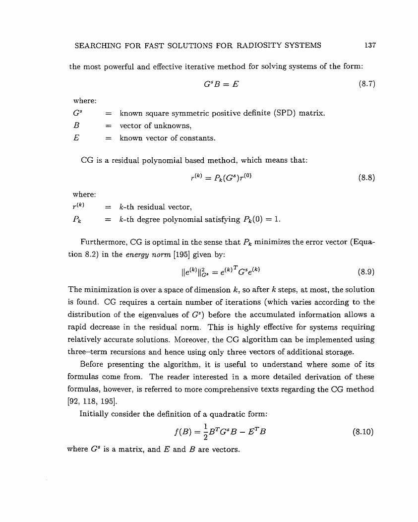
SEARCHING FOR FAST SOLUTIONS FOR MDIOSITY SYSTEMS 137
the most powerful and effective iterative met hod for solving systems of the form:
where:
Gs = known square syrnmetric positive definite (SPD) m a t r k
B = vector of unknowns?
E = known vector of constants.
CG is a residual polynomial based method, which mems that:
where: T ( k ) = k-th residual vector,
pk = k-th degree polynomial satisfying %(O) = 1.
Furthermore, CG is optimal in the sense that Pk minimizes the error vector (Equa-
tion 8.2) in the energy n o r m [195] given by:
The minimization is over a space of dimension k, so after k steps, at rnost, the solution
is found. CG requires a certain number of iterations (mhich vaxies according to the
distribution of the eigenvalues of Gs) before the accumulated information allows a
rapid decrease in the residual norm. This is highly effective for systems requiring
relatively accurate solutions. Moreover, the CG algorit hm can be implemented using
three-term recursions and hence using only three vectors of additional storage-
Before presenting the algorithrn, it is useful to understand where some of its
formulas corne from. The reader interested in a more detailed derivation of these
formulas, however, is referred to more comprehensive texts regarding the CG method
[92, 118, 1951.
Initially consider the definition of a quadratic fom:
1 f ( ~ ) = - B ~ G ~ B - E ~ B
2 (8.10)
where GS is a matrix, and E and B are vectors.
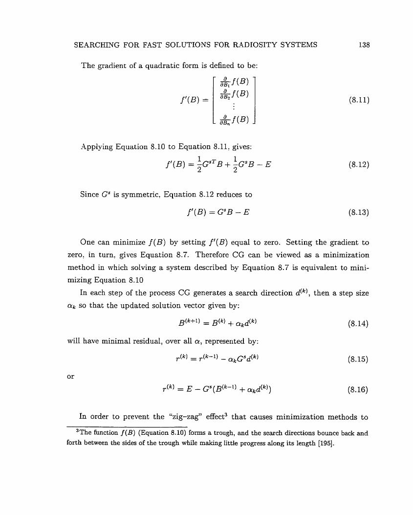
SEARCHING FOR FAST SOLUTIONS FOR RmIOSITY SYSTEMS
The gradient of a quadratic form is defined to be:
Applying Equation 8.10 to Equation 8.11; gives:
Since GS is symmetric, Equation 8.12 reduces to
f ' (B ) = GSB - E
One can minimize j ( B ) by setting f ' (B) equal to zero. Setting the gradient to
zero, in turn, gives Equation 8.7. Therefore CG can De viewed as a minimization
method in which solving a system described by Equation 8.7 is equivalent to mini-
mizing Equation 8.10
In each step of the process CG generates a search direction d(k) , then a step size
a k so that the updated solution vectûr given by:
will have minimal residual, over al1 a, represented by:
In order to prevent the "zigzag" effect3 that causes minimization methods to
3She function f (B) (Equation 8.10) foms a trough, and the search directions bounce back and
forth between the sides of the trough while makuig Little progress dong its length [195].
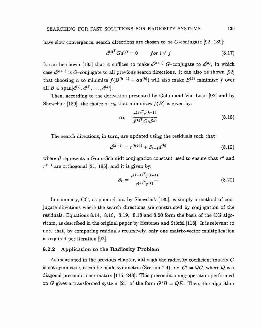
SE,kRCHn\lG FOR FAST SOLUTIONS FOR RADIOSITY SYSTEMS 139
have slow convergence, search directions are chosen to be G-conjugate [92, 1891:
Tt can be shown [195] that it suffices to make d('+') G-conjugate to d(k), in which
case d(k+L) is G-conjugate to al1 previous search directions. It c m also be shown [92]
that choosing a to rninirnize f ( B ( ~ - ~ ) f will also make B ( ~ ) minimimize f over
al1 B E span[d('). d('), . . . d(')].
Then. according to the derivation presented by Golub and Van Loan [92] and by
Shewchuk [189]. the choice of cuk that minirnizes f (B) is given by:
The search directions, in turn, are updated using the residuals such that:
where ,h' represents a Gram-Schmidt conjugation constant used to ensure that rk and
rk-' are orthogonal [210 1951, and it is given by:
In summary, CG, as pointed out by Shewchuk [Mg], is simply a method of con-
jugate directions where the search directions are constructed by conjugation of the
residuals. Equations 8.14, 8.16, 8.19, 8.18 and 8.20 f o m the basis of the CG algo-
rithm, as described in the original paper by Hestenes and Stiefel [ll8]. It is relevant to
note t hat , by computing residuals recursively, only one matrix-vector multiplication
is required per iteration [92].
8.2.2 Application to the Radiosity Problem
-4s mentioned in the previous chapter, although the radiosity coefficient matrix G
is not symmetric, i t can be made symmetric (Section '7.4), 2.e. GS = QG, where Q is a
diagonal preconditioner matrix [115, 2431. This preconditioning operation performed
on G gives a transforrned system 1211 of the form GsB = QE. Then, the algonthm
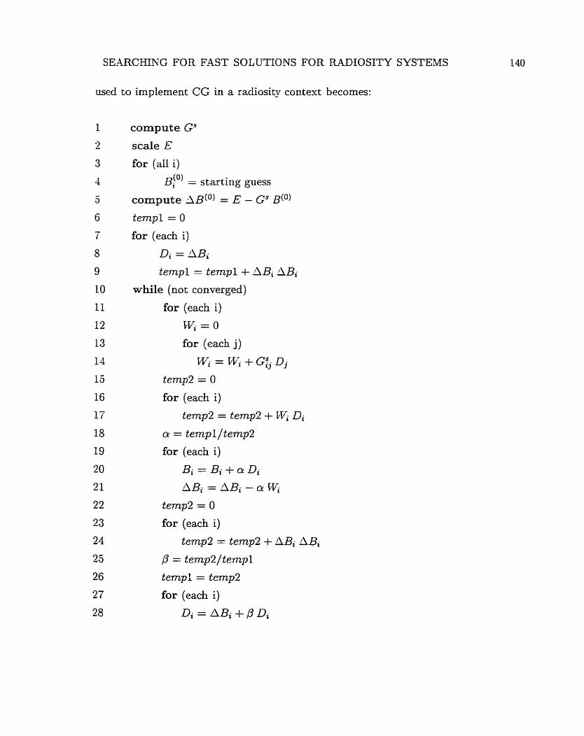
SEARCHING FOR FAST SOLUTIONS FOR RADIOSITY SYSTEMS
used to implement CG in a radiosity context becomes:
compute Gs
scale E for (al1 i)
B!') = starting guess
compute AB(') = E - Gs B ( O )
t e m p l = O
for (each i)
Di = /\Bi
t e m p l = t e m p l + ABi ABi
while (not converged)
for (each i)
bVi = O
for (each j)
T,Vi = LVi + Gij Dj
temp2 = O
for (each i)
tempS = t emp2 + Pc Di cr = t e m p l l t e m p 2
for (each i)
Bi = Bi + O! Di ABi = ABi - cr vvi
temp2 = O
for (each i)
t emp2 = t emp2 + ABi ABi
p = temp2/tel.npl
t e m p l = t empS
for (each i)
D i = A B i + p D i
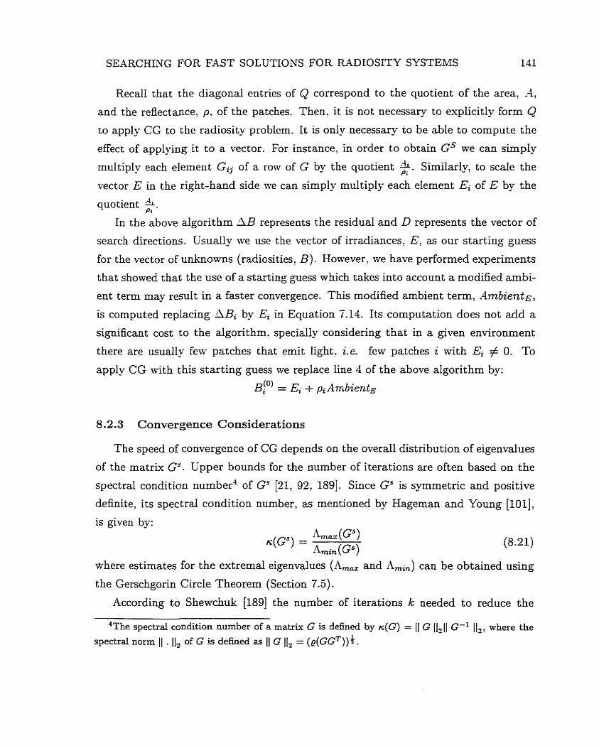
SEARCKING FOR FAST SOLUTIONS FOR RADIOSITY SYSTEMS 141
Recall that the diagonal entries of Q correspond to the quotient of the area; A,
and the reflectance, p, of the patches. Then, it is not necessary to explicitly form Q
to apply CG to the radiosity probiem. It is only necessary to be able to compute the
effect of applying it to a vector. For instancel in order to obtain G' we can simply
multiply each element Gij of a rom of G by the quotient $- Similarll to scale the
vector E in the right-hand side me can simply multiply each element Ei of E by the
quotient $. In the above algorithm AB represents the residual and D represents the vector of
search directions. Csually we use the vector of irradiances. E, as our starting guess
for the vector of unknowns (radiosities, B). However, we have perforrned experiments
that showed that the use of a starting guess which takes into account a modified ambi-
ent term may result in a faster convergence. This modified ambient term, AmbientE,
is computed replacing ABi by Ei in Equation 7.14. Its computation does not add a
significant cost to the algorithm, specia,lly considering that in a given environment
there are usudly few patches chat emit light. Le. fem patches i with Ei # O. To
apply CG with this starting guess we replace line 4 of the above algorithm by:
B,(') = Ei + piArnbientE
8.2.3 Convergence Considerations
The speed of convergence of CG depends on the overall distribution of eigenvalues
of the matrix GS. Upper bounds for the number of iterations are often based on the
spectral condition number4 of Gs [21, 92, 1891. Since Gs is symmetric and positive
definite, its spectral condition number, as mentioned by Hageman and Young [loi], gven by:
where estimates for the extrema1 eigenvalues (A,, and LI,,) can be obtained using
the Gerschgorin Circle Theorem (Section 7.5).
According to Shewchuk [189] the number of iterations k needed to reduce the
4The spectral condition number of a mat+ G is defined by K(G) = II G (1, II G-' II,, where the
spectral norm II . 11, of G is defùied as II G 11, = ( e ( ~ ~ T ) ) * .
SEARCHING FOR FAST SOLUTIONS FOR RADIOSITY SYSTEMS 142
residual by a factor of E in the energy n o n can be estimated by:
The relation above. based on Theorem 102.5 of Golub and Van Loan [92], infer
that the number of iterations is proportional to \~K(GJ) . However: if the extrema1
eigenvalues are well separated, CG can provide a superlinear convergence rate5 since it
implicitly builds up information about the spectrum of the matrix GS as its iterations
proceed. -4s mentioned by Barret e t al. [21], CG tends to eliminate the components
of the error in the direction of eigenwctors açsociated with extremd eigenvalues first.
After these have been eliminated, the method progressively moves towards the interior
of the region containing the spectrum, i.e. the convergence rate becomes dependent
on a reduced system with a srnaller condition number [65] .
It is not a pn'on clear that CG is optimal for radiosity systems, mhich require
low accuracy solutions with only a few sweeps through the matrix. The fact that the
radiosity matrices tend to have the eigenvalues tightly clustered around a few values
(section 8.62). however, suggests that upper bound for the number of iterations
needed for radiosity problems may be lower than the one given by the relation above.
We examine this issue in more detail in Section 8 - 6 2
8.3 Chebyshev Polynomials
Before introducing the Chebyshev met hod, ive need to present the definition and
main properties of the Chebyshev polynomials. These polynomials represent the basis
of the Chebyshev method, and the knowledge about their behavior is fundamental
for the analysis of the convergence of this iterative method.
The Chebyshev polynomials Y, [42] for the interval [-1,1] are defined by:
Y,(x) = cos[m cos-' (x)] for each m > O (8.23)
Since they are orthogonal with respect to the weight function
w(z) = (1 - x2)-Il2, they can be computed using the three terrn recursion:
5Convergence at a rate that increases per iteration f21, 581.
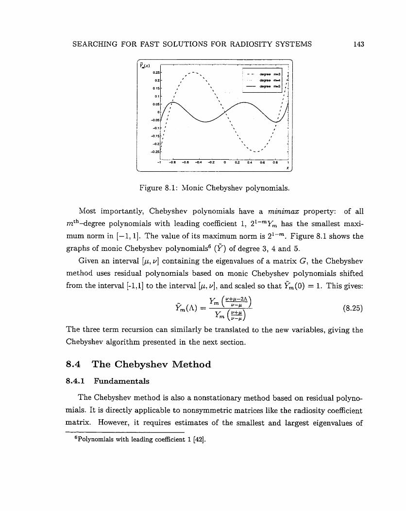
SEARCHING FOR FAST SOLUTIONS FOR RADIOSITY SYSTEMS
Figure 8.1 : Monic Chebyshev po l~omia l s .
Most importantly, Chebyshev polj-nomials have a rninimax property: of al1
mth-degree polpomials with leading coefficient 1; 2'-"Ym has the smallest maxi-
mum norm in [-1,1]. The value of its maximum norm is Pm. Figure 8.1 shows the
graphs of monic Chebyshev polynomiaIs6 (Y) of degree 3, 4 and 5.
Given an interval [P, v] containing the eigenvalues of a matrix G. the Chebyshev
method uses residual polynomials based on monic Chebyshev polynomials shifted
from the interval [-1.11 to the interval [p? v], and scaled so that Fm (O) = 1. This gives:
Ym Fm (A) = Ym (z)
The three term recursion can sirnilady be translated to the new variables, giving the
Chebyshev algorithm presented in the next section.
8.4 The Chebyshev Method
The Chebyshev method is also a nonstationary method based on residual polyno-
mials. It is directly applicable to nonsymmetric matrices like the radiosity coefficient
matrix. Homever, it requires estimates of the smallest and largest eigenvalues of
6Polynomials wit h leading coefficient 1 [42].
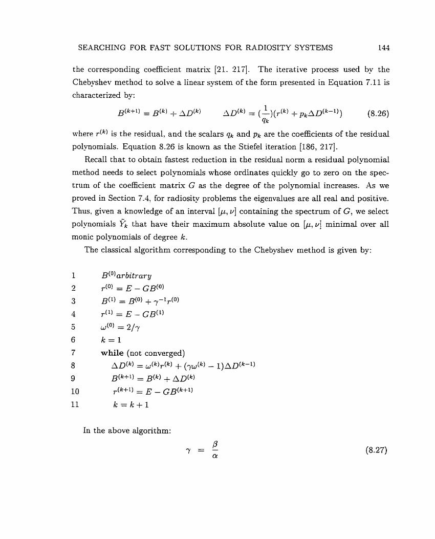
SEARCHING FOR FAST SOLUTIONS FOR RADTOSITY SYSTEMS 14-?
the corresponding coefficient matrix [21. 21'71. The iterative process used by the
Chebyshev method to solve a linear system of the form presented in Equation 7-11 is
characterized by:
mhere dk) is the residual, and the scalars q k and pk are the coefficients of the residual
po l~omia l s . Equation 8.26 is known as the Stiefel iteration [186, 2171.
Recall that to obtain fastest reduction in the residual norm a residual p o l ~ o m i a l
method needs to select polynomials whose ordinates quickly go to zero on the spec-
trum of the coefficient matrix G as the degree of the polynomial increases. As we
proved in Section 7.4: for radiosity problerns the eigenvalues are al1 real and positive.
Thus, given a knowledge of an interval [p, v] containing the spectrum of Gy we select
polynomials that have their rnasirnum absolute value on [P, u] minimal over al1
monic polynomials of degree k.
The classical algorithm corresponding to the Chebyshev method is given y - :
In the above algorithm:
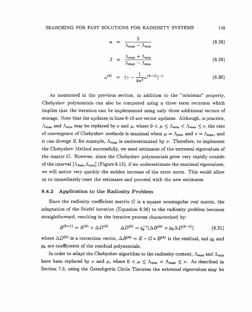
SEARCHING FOR FAST SOLUTIONS FOR RADIOSITY SYSTEMS 145
As mentioned in the previous section, in addition to the ~ 7 m i n i m ~ 7 ' property?
Chebyshev polynonials can also be computed using a three term recursion which
implies that the iteration can be irnplemented using only three additional vectors of
storage. Note that the updates in lines 8-10 are vector updates. Although, in practice,
A,, and ilmin rnay be replaced by v and p, where O < /I 5 Ami, < A,, 5 v, the rate
of convergence of Chebyshev methods is maximal when p = and v = A,,, and
it can diverge if. for example, A,, is underestimated by v. Therefore, to implement
the Chebyshev Method successfully, we need estimates of the extrema1 eigenvalues of
the matriu G. However, since the Chebyshev polynomiais grow very rapidly outside
of the interval [i\mu,ilmin] (Figure 8-13), if Ive underestimate the maximal eigenvalues,
we will notice very quickly the sudden increase of the error norrn. This would allow
us to immediately reset the estimates and proceed wïth the new estimates.
8.4.2 Application to the Radiosity Problem
Since the radiosity coefficient matriv G is a square nonsingular real matrix. the
adaptation of the S tiefel iteration (Equation 8.26) to the radiosity problem becomes
straightfomard, resulting in the iterative process characterized by:
where AD(') is a correction vector, AB(^) = E - G * B ( ~ ) is the residual, and qk and
pk are coefficients of the residual polynomials.
In order to adapt the Chebyshev algonthm to the radiosity context, A,, and Amin
have been replaced by u and p, where O < p 5 Amin c A,, 5 u. As described in
Section 7.5, using the Gerschgorin Circle Theorem the extrema1 eigenvalues may be
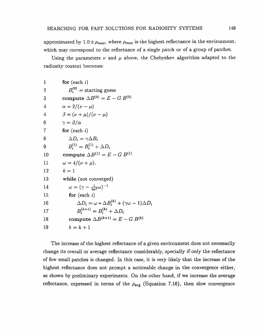
SEARCHING FOR FAST SOLUTIONS FOR FUDIOSITY SYSTEMS 146
approximated by 1.0 i. p,,: where Pm, is the highest reflectance in the environment-
which may correspond to the reflectance of a single patch or of a group of patches.
Csing the parameters v and ,u above- the Chebyshev algorithm adapted to the
radiosity context becomes:
for (each i)
~ 1 ' ) = start ing guess
compute AB(') = E - G B(O)
Cr = 2 / ( u - p )
P = (u + d / ( v - P) = p/a
for (each i)
I D i = -/ABi fjy = Bi1) -+ ADi
compute ilB(l) = E - G B(')
w = 4 / ( v + p ) .
k = l
while (not converged)
'J = (7 - L w ) - L 4 ~ '
for (each i)
ADi = w r AB,(") + ( y u - i)ADi @k+ 1) - - B!"' + ADi
compute AB("') = E - G B ( ~ )
k = k + l
The increase of the highest reflectance of a given environment does not necessarily
change its overall or average reflectance considerably. specially if only the reflectance
of few small patches is changed. In this case, it is very likely tha t the increase of the
highest reflectance does not prompt a noticeable change in the convergence either,
as s h o w by preliminary experiments. On the other hand, if we increase the average
reflectance, expressed in terms of the p,,, (Equation 7.16), then slow convergence
SEARCMNG FOR F-4ST SOLUTIONS FOR RADIOSITY SYSTEMS 147
results. Since the increase of the highest reflectance may not change the average
reflectance considerabl- as we described above, we performed esperiments using pavg
instead of p,,, to estimate the eigenvdues. The better results obtained for al1 the
cases tested (Section 8-5.2): determined the folloming choice of Chebyshev parameters:
In al1 the cases tested, the use of a starting guess which takes into account the
modified arnbient term, -4mbientE (section 8.2-2): gives better results than a starting
guess which uses only the vector of ernittances. To use this starting guess we replace
line 2 of the above algorithm by-:
B!') = Ei + piAmbientE
8.4.3 Convergence Considerat ions
Heuristically, we can compare the CG and Chebyshev methods in terms of their
underlying residual polynomials [21]. For CG the polynomials tend to rapidly con-
verge to zero at the extrema1 eigenvalues? then progressively move towards the interior
of the region containing the spectrum, zeroing out eigenvalues as iterations proceed.
Chebyshev polynomials tend to uniformly drive al1 the eigenvalues to zero a t the same
rate. For solutions requiring high accuracy, the CG algorithm is usually the faster
of the two since it implicitly creates the "optimal" polynomial on each step. For the
low accuracy solutions needed in radiosity, however: it is more important to quickly
reduce the residual corresponding t o al1 the eigenvalues. So we expect the Chebyshev
iteration to be faster, which is borne out by the testing results presented in the next
section.
8.5 Testing Parameters and Procedures
We compared the following algorithms, using explicitly stored form factors:
Gauss-Seidel (GS) described in Section 7.2.1,
Standard Progressive Refinement (PR) described in Section 7.2.3,
SEARCHING FOR FAST SOLUTIONS FOR RADIOSITY SYSTEMS
Overshooting (FEDA) described in Section 7.2.4.
Conjugate Gradient (CG) described in Section 8.2:
Chebyshev (CHEBY) described in Section 8.4.
The starting guesses were chosen in order to obtain the best possible rate of
convergence for each tested algorithm. Consequently, the initial error norm is not
the same for curves on a single graph. The starting guess used for Gauss-Seidel and
Conjugate Gradient algorithms was the vector of ernittances and for the radiosity-
specific methods we used a vector of zeros. For the Chebyshev algonthm we used the
starting guess given by B!') = Ei + piArnbientE (Section 8.4.2).
8-5.1 Performance Measmement
The general matriu methods check the convergence after a complete sweep of
the coefficient mat rk , i. e. one iteration. The radiosity-specific methods perform this
check after one relaxation step, i-e. one step of iteration. To make our measurement
comparable we count steps of iteration. In this context an iteration of a general mat rk
method corresponds to n steps of iteration, where n is the order of the coefficient
matriu.
To mesure the time we start the dock at the beginning of a cycle of k steps of
iteration, and stop it after k steps of iteration. For the general matrix methods tested
we use k = n. We check for k a t each step in order to make the timing overhead
the same for al1 ~ e t h o d s . In addition, the error norm used as stopping criterion is
computed outside of the timing cycles. The time measurements are given by elapsed
CPU time on a SGI Challenge ('70-R4400). -411 the algorithms were implemented
using the same software guidelines to avoid differences that could affect the timing.
8.5.2 Test Cases
The test scene used in our expenments consists of a sphere centered in a "Corne11
box" (Figure 8.2). The sphere was divided into 128 patches and the faces of the
surrounding cube were divided into 144 patches forming a total of 992 patches. The
light source corresponds to 16 patches on the center of the box "ceiling" (face 6). The
values used for d and h were 3.0 and 6.0 respectively.
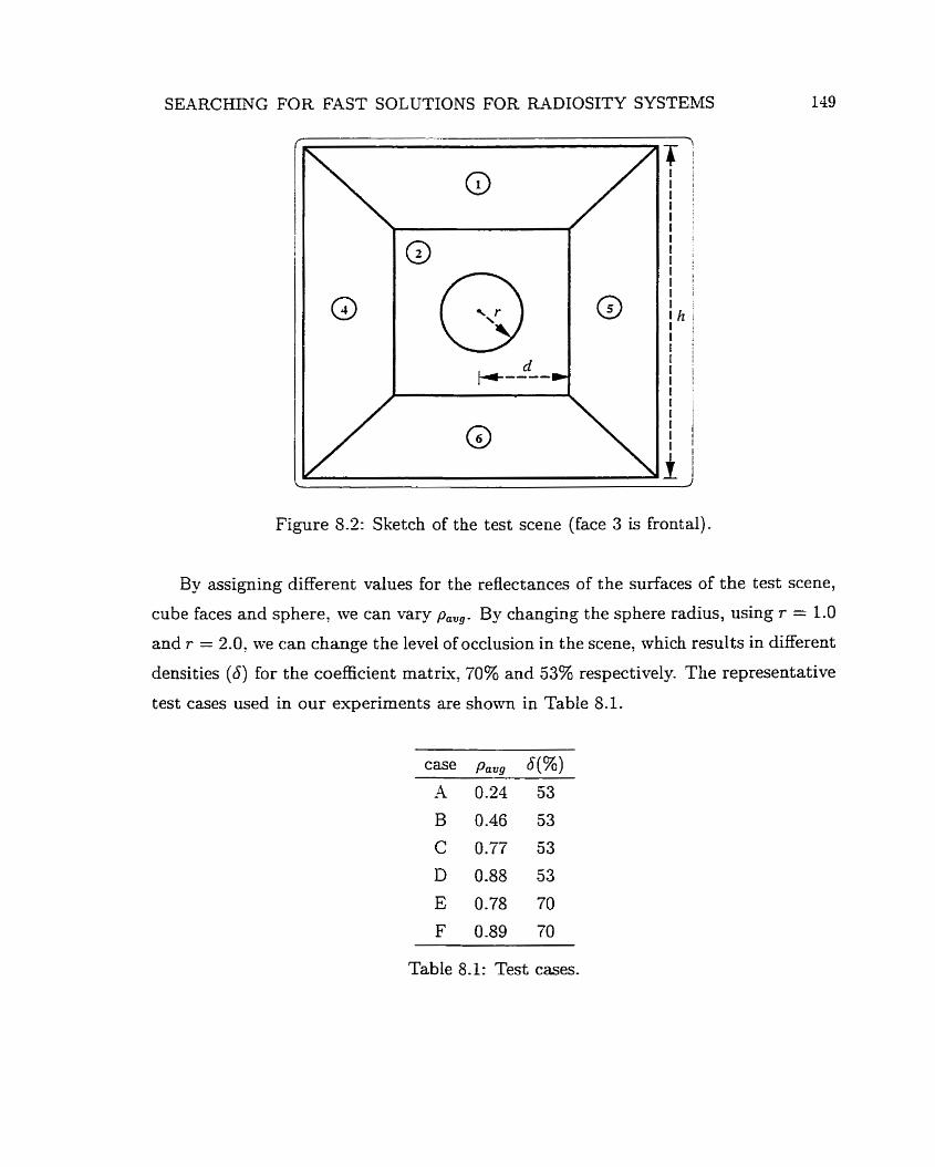
SEARCHING FOR F-4ST SOLUTIONS FOR RkDIOSITY SYSTEMS
Figure 5.2: Sketch of the test scene (face 3 is frontal).
By assigning different values for the reflectances of the surfaces of the test scene,
cube faces and sphere, we can Vary p,,, . By changing the sphere radius, using r = 1.0
and r = 2 -0' we can change the level of occlusion in the scene, which results in different
densities (6) for the coefficient matrk, 70% and 53% respectively. The representative
test cases used in Our experiments are shown in Table 8.1.
Table 8.1: Test cases.
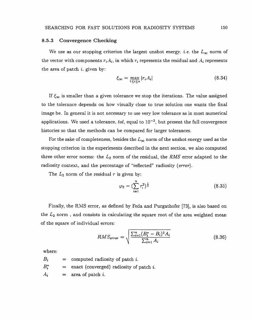
SEARCHIXG FOR F,ilST SOLUTIONS FOR RADIOSITY SYSTEMS
8.5.3 Convergence Checking
We use as our stopping criterion the Iargest unshot energu. i.e. the L, norm of
the vector with components in which ri represents the residual and -Ai represents
the area of patch i. aven by:
= max l ~ ~ a 4 ~ l 1 <i<n
(8.34)
If cm is smaller than a given tolerance we stop the iterations. The value assigned
to the tolerance depends on how vïsualiy close to tme solution one wants the final
image be. In general it is not necessary to use very low tolerance as in most numerical
applications. We used a tolerance' tol, equal to 10-37 but present the full convergence
histories so that the methods can be compared for larger tolerances.
For the sake of completeness, besides the L, norm of the unshot energy used as the
stopping criterion in the experiments described in the ne-* section: we also computed
three other error norms: the Lp norm of the residual, the RMS error adapted to the
radiosity context: and the percentage of "reflected" radiosity ( e n o r ) .
The L2 norm of the residual r is given by:
Finally, the RMS error, as defined by Feda and Purgathofer [73], is also based on
the L2 n o m , and consists in calculating the square root of the area weighted mean
of the square of individual errcrs:
where:
Bi = computed radiosity of patch i. Bi' = exact (converged) radiosity of patch i.
Ai = area of patch i.
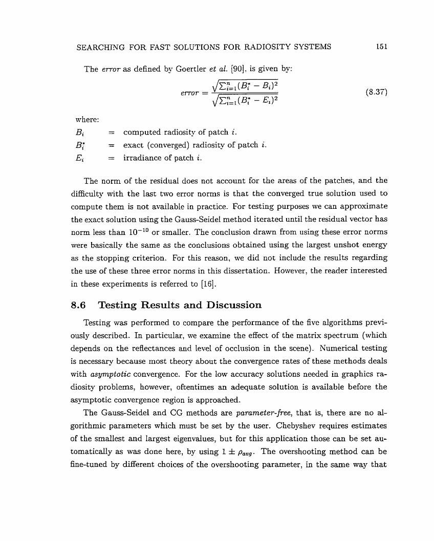
SEARCHIA-G FOR FAST SOLUTIONS FOR RADIOSITY SYSTEMS
The e r ro r as defined by Goertler et al. [go]? is given by:
where:
Bi = computed radiosity of patch i.
B: = exact (converged) radiosity of patch i.
Ei = irradiance of patch i.
The norm of the residual does not account for the areas of the patches, and the
difficulty with the last two error norms is that the converged true solution used to
compute them is not available in practice. For testing purposes we can approximate
the exact solution using the Gauss-Seidel method iterated until the residual vector has
norm less than 1 0 - ' O or smaller. The conclusion drawn from using these error norms
were basically the same as the conclusions obtained using the largest unshot energy
as the stopping criterion. For this reason, we did not include the results regarding
the use of these three error noms in this dissertation. However? the reader interested
in these experiments is referred to [16].
8.6 Testing Results and Discussion
Testing was performed to compare the performance of the five algorithms previ-
ously described. In pa.rticular, Ive examine the effect of the matrix spectrum (which
depends on the reflectances and Level of occliision in the scene). Numerical testing
is necessary because rnost theor-y about the convergence rates of these methods deals
with asymptotic convergence. For the low accuracy solutions needed in graphics ra-
diosity problerns, hotvever, oftentimes an adequate solution is available before the
asymptotic convergence region is approached-
The Gauss-Seidel and CG methods are pa~ameter-free, that is, there are no al-
gorithmic parameters which must be set by the user. Chebyshev requires estimates
of the smallest and largest eigenvalues, but for this application those can be set au-
tomatically as was done here, by using I f p,,,. The overshooting method can be
fine-tuned by different choices of the overshooting parameter, in the same way that
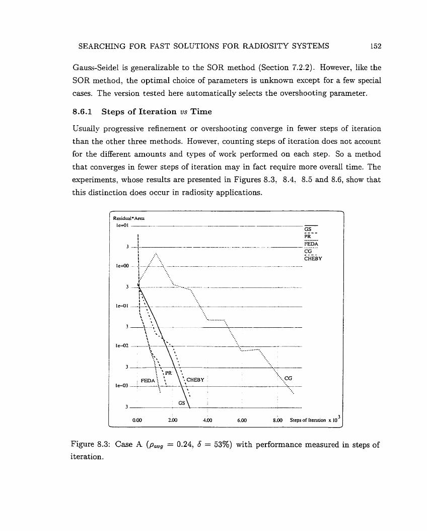
SEARCmG FOR FAST SOLUTIONS FOR RADIOSITY SYSTEMS
Gauss-Seidel is generalizable to the SOR method (Section 7.22)- However, N e the
SOR method, the optimal choice of parameters is u n k n o m except for a few specid
cases. The version t ested here automatically selects the overshooting parameter.
8.6.1 Steps of Iteration us Time
Csually progressive refinement or overshooting converge in feiver steps of iteration
than the other three methods. However: counting steps of iteration does not account
for the different amounts and types of ivork performed on each step. So a rnethod
that converges in fewer steps of iteration may in fact require more overall time. The
experiments, whose results are presented in Figures 8.3, 8.4, 8.5 and 8.6, show that
t his distinction does occur in radiosity applications.
0.00 700 4.00 6-00 8.00 Stcps of Itention x 10 3
Figure 8.3: Case -4 (p,,, = 0.24, 6 = 53%) with performance measured in steps of
iteration.
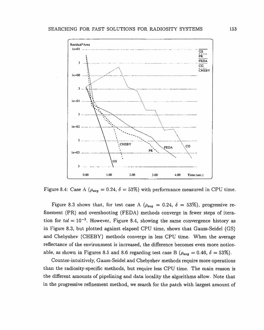
SEARCHING FOR FAST SOLUTIONS FOR MDIOSITY SYSTEMS
Figure 8.4: Case A (p.,, = 0.24; 6 = 53%) with performance measured in CPU time.
Figure 8.3 shows that, for test case A (p.,, = 0.24, 6 = 53%), progressive re-
finement (PR) 2nd overshooting (FEDA) methods converge in fewer steps of itera-
tion for tol = IO? However, Figure 8.4, showing the same convergence history as
in Figure 8.3, but plotted against elapsed CPCT time, shows that Gauss-Seidel (GS)
and Chebyshev (CHEBY) methods converge in less CPU time. When the average
reflectance of the environment is increased, the difference becomes even more notice-
able, as shown in Figures 8.5 and 8.6 regarding test case B (p., = 0.46, 6 = 53%).
Counter-intuitively, Gauss-Seidel and Chebyshev methods require more operations
than the radiosity-specific methods, but require less CPU time. The main reason is
the different amounts of pipelining and data Iocality the algorithrns allow. Note that
in the progressive refinement rnethod, we search for the patch with largest amount of
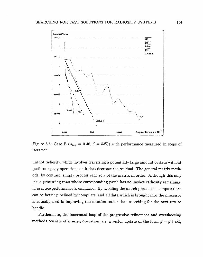
SEARCHING FOR FAST SOLUTIONS FOR MDIOSITY SYSTEMS
0.00 5.00 10.00 Steps of Iteraüan x 10 3
Figure 8.5: Case B (p,,, = 0.46, 6 = 53%) with performance measured in steps of
iteration.
unshot radiosity. which involves traversing a potentially large amount of data without
performing any operations on it that decrease the residual. The general m a t r k meth-
ods, by contrast, simply process each row of the rnatrix in order. Although this may
mean processing rows whose corresponding patch has no unshot radiosity remaining,
in practice performance is enhanced. By avoiding the search phase, the computations
can be better pipelined by compilers, and d l data which is hrought into the processor
is actually used in improving the solution rather than searching for the next row to
handle.
Furthermore, the innermost loop of the progressive refinement and overshooting
methods consists of a s q y operation, Le. a vector update of the form y'= y'+ CG,
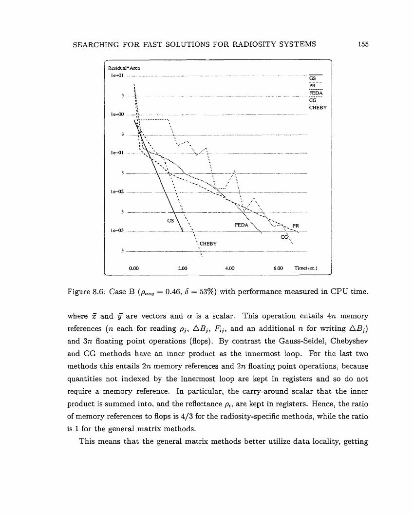
SEARCHING FOR FAST SOLUTIONS FOR RADFOSITY SYSTEMS
t
. CHEBY
Figure 8.6: Case B (p,, = 0.46, 6 = 53%) with performance measured in CPU tirne.
where iE and i j are vectors and ar is a scalar. This operation entails 4n m e m o l
references (n each for reading p j , ABj , Fi,, and an additional n for writing ABj)
and 3n Boating point operations (flops). By contrat the Gauss-Seidel, Chebyshev
and CG methods have an inner product as the innermost loop. For the last two
methods this entails 2n memory references and 271 floating point operations; because
quantities not indexed by the innermost loop are kept in registers and so do not
require a rnemory reference. In particular, the carry-around scalar that the inner
product is summed into, and the reflectance pi, are kept in registers. Hence, the ratio
of memory references to flops is 4/3 for the radiosity-specific methods, while the ratio
is 1 for the general rnatrix methods.
This means that the general rnatrix methods better utilize data locality, getting
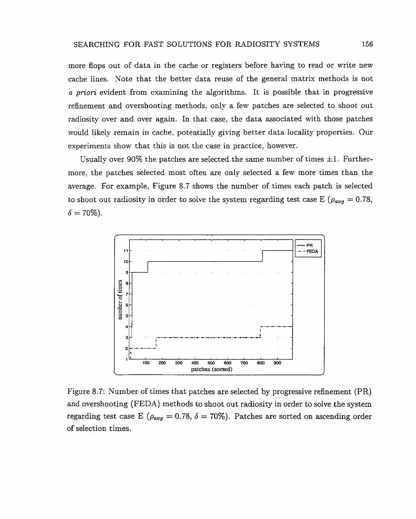
SEARCHING FOR FAST SOLUTIONS FOR RWIOSITY SYSTEMS 156
more Bops out of data in the cache or registers before having to read or m i t e new
cache lines. Note that the better data reuse of the general rnatrix methods is not
a priori evident from evamining the algorithms. It is possible that in progressive
refinement and overshooting methods, onIy a few patches are seIected to shoot out
radiosity over and over again. In that case, the data associated with those patches
would likely remain in cache? potentially giving better data locality properties. Our
experiments show that this is not the case in practice, hoivever.
L'sually over 90% the patches are selected the same number of times Il. Further-
more, the patches selected most often are only selected a few more times than the
average. For exampIe, Figure 8.7 shows the nurnber of times each patch is selected
to shoot out radiosity in order to solve the system regarding test case E (p,,, = 0.78:
6 = 70%).
100 200 300 400 500 soo 700 a00 wo patches (sorted)
Figure 8.7: Number of times that patches are selected by progressive refinement (PR) and overshooting (FEDA) methods to shoot out radiosity in order to solve the system
regarding test case E (p,, = 0.78, 6 = 70%). Patches are sorted on ascending order
of selection times.
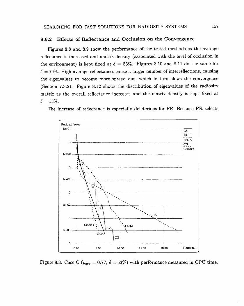
SEARCHING FOR FAST SOLUTIONS FOR RADIOSITY SYSTEMS
8.6.2 Effects of Reflectance and Occlusion on the Convergence
Figures 8.8 and 8.9 show the performance of the tested methods as the average
reflectance is increased and matriy density (associated nrit h the level of occlusion in
the environment) is kept hed at P = 53%. Figures 8-10 and 8.11 do the same for -
6 = (0%. High average reflectances cause a larger number of interreflections, causing
the eigenvalues to become more spread out: which in turn slows the convergence
(Section T.3.2). Figure 8.12 shows the distribution of eigenvalues of the radiosity
rna t r i~ as the overall reflectance increases and the matris density is kept fked a t
s = 33%.
The increase of reflectance is especially deleterious for PR. Because PR selects
Figure 8.8: Case C (p,, = 0.77, b = 53%) with performance measured in CPU tirne.
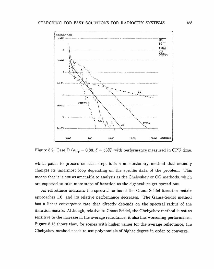
SEARCHING FOR FAST SOLUTIONS FOR RADIOSITY SYSTEMS
Figure 8.9: Case D (p,,, = 0.88, 6 = 53%) with performance rneasured in CPU time.
which pateh to process on each step, it is a nonstationary method that actually
changes its innermost loop depending on the specific data of the problem. This
means that it is not as amenable to analysis as the Chebyshev or CG methods, which
are expected to take more steps of iteration as the eigenvalues get spread out.
As reflectance increases the spectral radius of the Gauss-Seidel iteration matrix
approaches 1.0, and its relative performance decreases. The Gauss-Seidel method
has a linear convergence rate that directly depends on the spectral radius of the
iteratiun matriu. Although, relative to Gauss-Seidel, the Chebyshev method is not as
sensitive to the increase in the average reflectance, it also has worsening performance.
Figure 8.13 shows that, for scenes with higher values for the average reflectance, the
Chebyshev method needs to use polynomials of higher degree in order to converge.
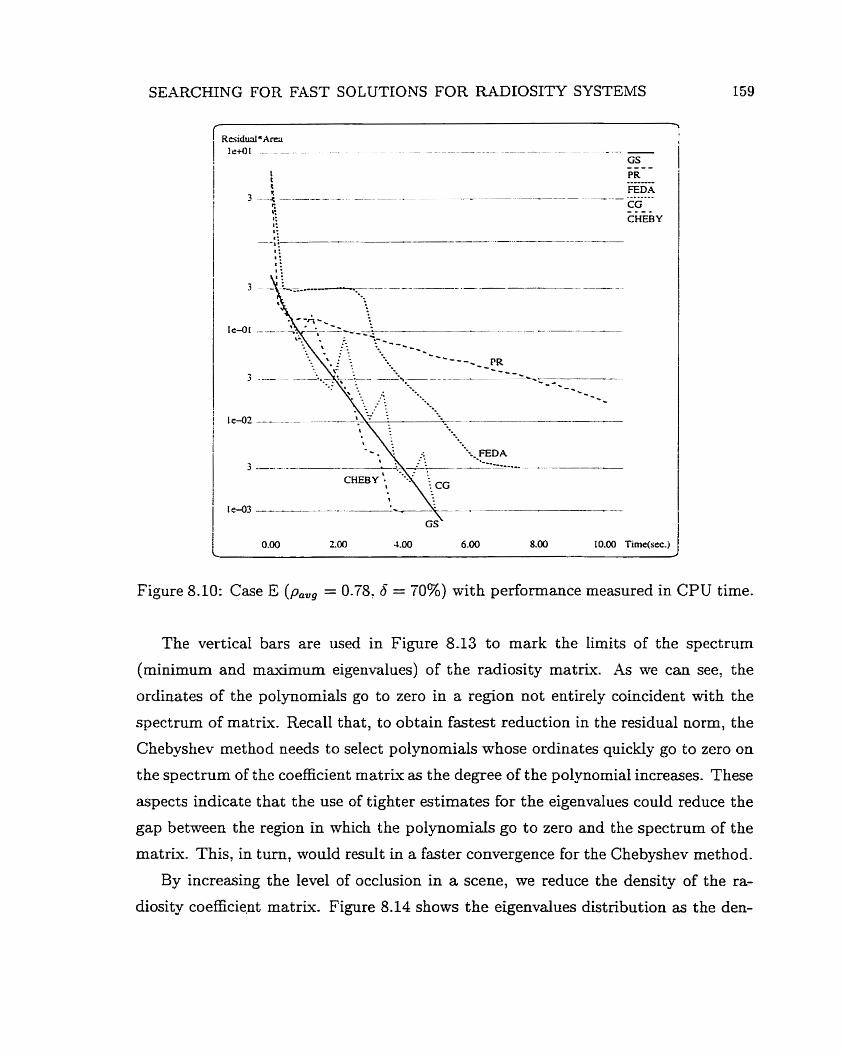
SEARCHING FOR FAST SOLUTIONS FOR RADIOSITY SYSTEMS
- - - - CHEBY
Figure 8.10: Case E (paVg = 0.78, 6 = 70%) with performance measured in CPU time.
The verticai bars are used in Figure 8.13 to mark the limits of the spectrum
(minimum and maximum eigenvalues) of the radiosity mat+. As we can see, the
ordinates of the polynomials go to zero in a region not entirely coincident with the
spectmm of matrix. Recall that, to obtain fastest reduction in the residual norm, the
Chebyshev method needs to select polynomials whose ordinates quickly go to zero on
the spectrum of the coefficient matrk as the degree of the polynomial increases. These
aspects indicate that the use of tighter estimates for the eigenvalues could reduce the
gap between the region in which the polynomials go to zero and the spectrum of the
matrix. This, in turn, would result in a faster convergence for the Chebyshev method.
By increasing the level of occlusion in a scene, Rie reduce the density of the ra-
diosity coefficient matrix. Figure 8.14 shows the eigenvalues distribution as the den-
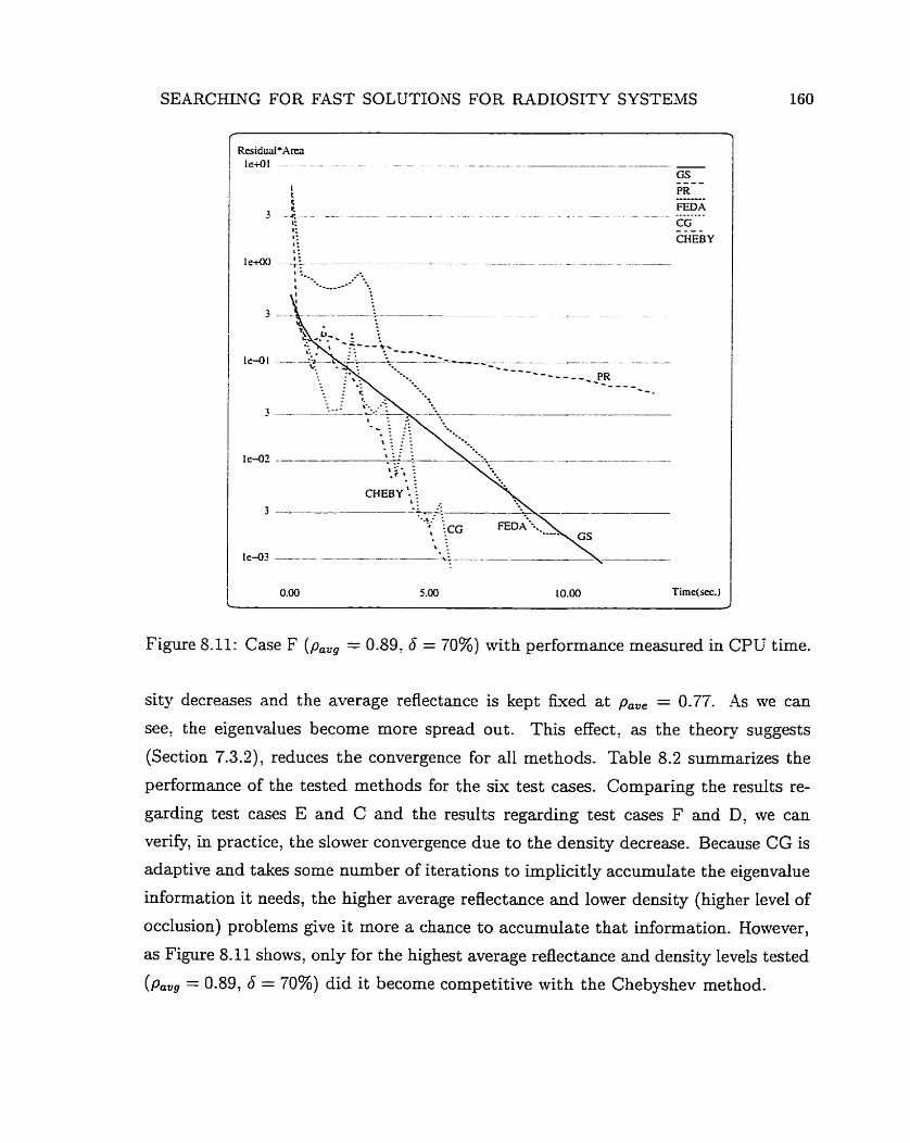
SEARCHING FOR FAST SOLUTIONS FOR RADIOSITY SYSTEMS
Figure 8.11: Case F (p,,, = 0.89: 6 = 70%) with performance measured in CPU time.
sity decreases and the average reflectance is kept fked at pave = 0.77. As we can
see, the eigenvalues become more spread out. This effect, as the theory suggests
(Section 7.3.2), reduces the convergence for dl methods. Table 8.2 summarizes the
performance of the tested methods for the six test cases. Comparing the results re-
garding test cases E and C and the resuIts regarding test cases F and D, we can
verify, in practice, the slower convergence due to the density decrease. Because CG is
adaptive and takes some number of iterations to implicitly accumulate the eigenvalue
information it needs, the higher average reflectance and lower density (higher level of
occlusion) problerns give it more a chance to accumulate that information. However,
as Figure 8.11 shows, only for the highest average reflectance and density levels tested
(pav, = 0.89, 6 = 70%) did it become competitive with the Chebyshev method.
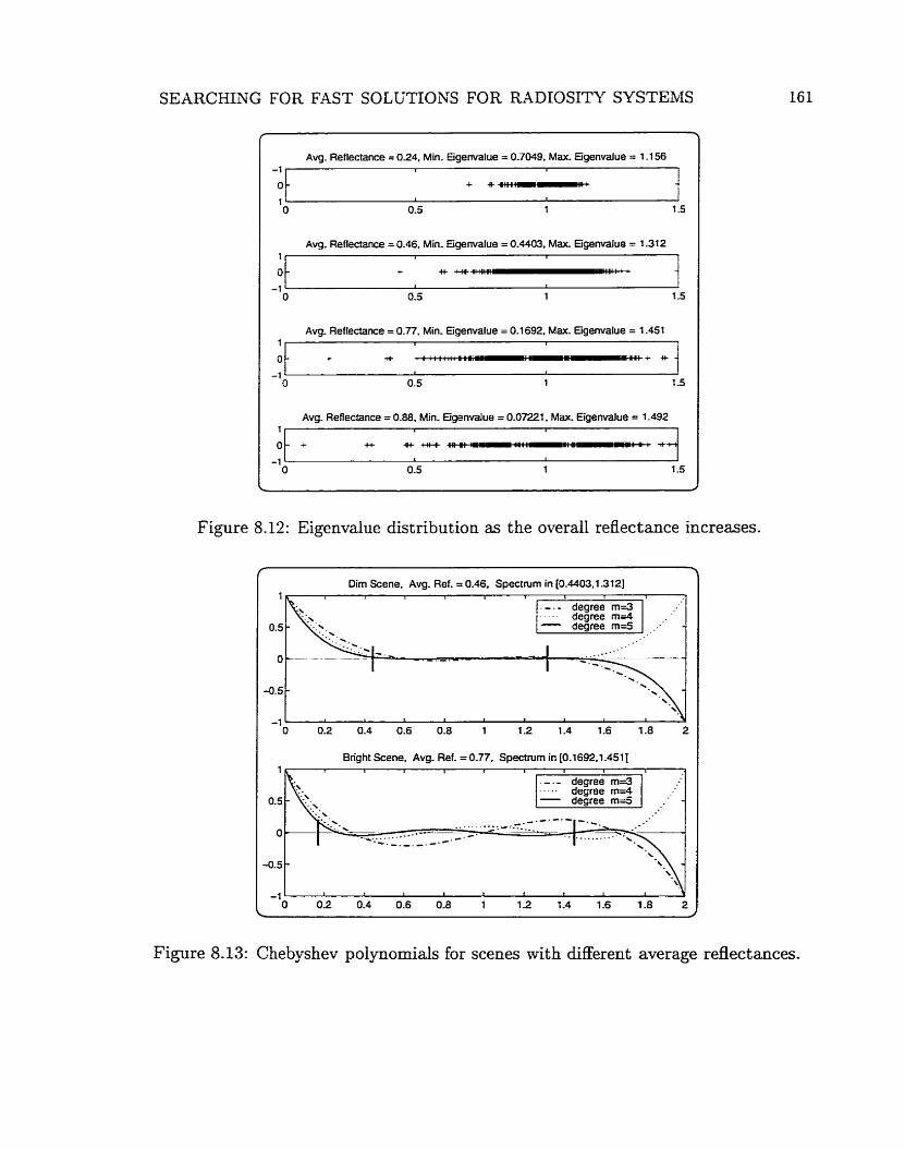
SEARCHING FOR FAST SOLUTIONS FOR MDIOSITY SYSTEMS
Avg. Reflectance = 024. Min- Eigenvalue = 0.7049. Max. Eigenvalue = 1.1 56 1 1
Avg. Reflectance = û.46. Min- Eigenvalue = 0.4403. M a x Eigenvalue = 1.312 f
Avg. Reflectance = 0.77. Min- Eigenvalue = 0.1692. Max Eigenvalue = 1.451
1
1 Avg. Reflecfance = 0.88. Min. Egenvaiue = 0.07221. Max. Eigenvalue = 1.492 1 1 1
Figure 8.12: Eigenvalue distribution as the overall reflectance increases.
Dim Scene. Avg. Ref. = 0.46. Spectmm in [0.4403.1.312]
Bright Scene. Avg. Ref. = 0.77. Spectnim in [0.1692.1.451I r 1 I I I 1 I I
. - . - degree m=3
..... degme m=4
Figure 8.13: Chebyshev polynomials for scenes with different average reflectances.
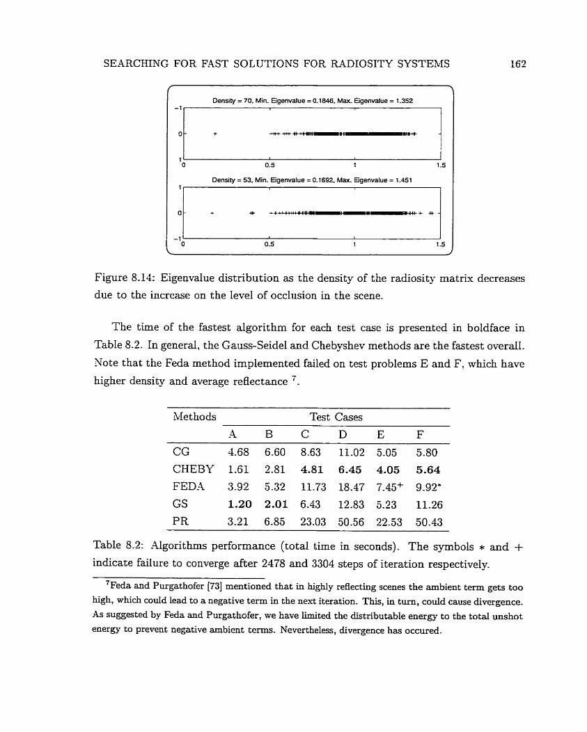
SEARCHING FOR FAST SOLUTIONS FOR RADIOSITY SYSTEMS 162
Oensity = 53. Min. Eigenvalue = 0.1692. Max- Eigenvalue = 1.451 1
Density = 70. Min. Eigenvalue = 0.1 846. Max. Eigenvalue = 1.352
Figure 8.14: Eigenvalue distribution as the density of the radiosity matrix decreases
- 1
0 -
1
due to the increase on the level of occlusion in the scene.
1
+ ***
The time of the fastest algorithm for each test case is presented in boldface in
O 0.5 1 1.5
Table 8.2- In general, the Gauss-Seidel and Chebyshev methods are the fastest overall.
Xote that the Feda method implemented failed on test problems E and F, which have
higher density and average reflectance '.
Met hods Test Cases
CG 4.68 6.60 8.63 11.02 5.05 5.80
CHEBY 6 1 2.81 4.81 6.45 4-05 5.64
FEDA 3.92 5.32 11.73 18.47 7.45* 9.92*
GS 1.20 2.01 6.43 12.83 5-23 11.26
PR 3.21 6.85 23.03 50.56 22.53 50.43
Table 8.2: Algorithms performance (total time in seconds). The symbols * and + indicate failure to converge after 2478 and 3304 steps of iteration respectively.
'Feda and Purgathofer [73] mentioned that in highiy reflecting scenes the ambient term gets too
high, which could lead to a negative term in the ne-xt iteration. This, in tuni, could cause divergence.
-4s suggested by Feda and Purgathofer, we have limited the distributable energy to the total unshot
energy to prevent negative ambient terms. Nevert heless, divergence has occured.
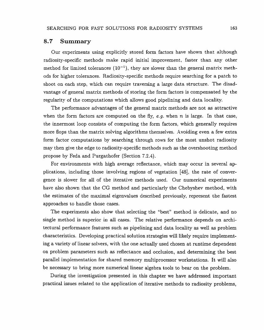
SEARCHING FOR FAST SOLUTIONS FOR RADIOSITY SYSTEhIS 163
8.7 Summary
Our esperiments using esplicitly stored form factors have s h o m that although
radiosity-specific rnethods make rapid initial improvement, faster than any other
method for limited tolerances (10-~) they are slower than the general matnlc meth-
ods for higher tolerances. Radiosit-specific methods require searching for a patch to
shoot on each step, svhich can require traversing a large data structure- The disad-
vantage of general rnatriv methods of storing the form factors is compensated by the
regularity of the computations which allows good pipelining and data locality.
The performance advantages of the general matrix methods are not as attractive
when the form factors are computed on the fiy, e.g. when n is large. In that case,
the innermost loop consists of computing the form factors, which generally requires
more flops than the matris solving algorithms themselves. Avoiding even a few extra
form factor computations by searching through rows for the most unshot radiosity
may then give the edge to radiosity-specific methods such as the overshooting method
propose by Feda and Purgathofer (Section 7.2.4).
For environments with high average reflectance, which may occur in several a p
plications, including those involving regions of vegetation [48], the rate of conver-
gence is slower for al1 of the iterative methods used. Our numencal experiments
have also shown that the CG method and particularly the Chebyshev method, with
the est imat es of the maximal eigenvalues descnbed previously, represent the fast est
approaches to handle those cases.
The experiments also show that selecting the "best" method is delicate, and no
single method is supenor in dl cases. The relative performance depends on archi-
tectural performance features such as pipelining and data locality as well as problem
characteristics. Developing practical solution strategies Nil1 likely require implement-
ing a variety of linear solvers, with the one actually used chosen a t runtime dependent
on problem parameters such as reflectance and occlusion, and detemining the best
parallel implementation for shared mernory multiprocessor workstations. It will also
be necessary to bring more numerical linear algebra tools to bear on the problem.
During the investigation presented in this chapter we have addressed important
practical issues related to the application of iterative methods to radiosity pro blems,

SEARCKLNG FOR FAST SOLUTIONS FOR RADIOSITY SYSTEMS 164
such as convergence conditions and stopping criteria. We have also pointed out that
iterative methods can have a better performance with different choices of initial a p
proximation for the solution vector. IntuitiveIy we may say that the closer the initial
approximation, the faster the iterative method will converge8. The problem is how
to corne up with a closer initial approximation Nithout knowing the tme solution be-
fore hand, Le. solving the systern. In Appendk C we present experiments, in which
eigenvectors are used as solution vectors in graphics settings. that that may lead to
a solution for this problem in the radiosity conte*.
'There are methods, such as the Conjugate Gradient Squared (CGS) [21], that tend to diverge
if the initial approximation is close to the solution.

CHAPTER 9
Conclusions
9.1 Summary of Contributions
Recent developments in physicall-based rendering have provided very realistic
images of a vanety of environments composed mostly of inorganic materials. This
dissertation aimed to extend physically-based rendering to some organic materials.
Specifically. biologically and physically-based BDF models for plants were introduced.
Moreover, as Ive discussed in the introduction in Chapter 1. there is an important
interplay between local and global illumination, which affects the versatility, accuracy
and efficiency of the rendering methods directly. Considering this aspect, in this dis-
sert ation, instead of focusing only on local illumination issues related to BDF models
(Cha~ters 4 to 6 ) : we also investigated solutions for global illumination problems
(Chapters 7 and 8). More specifically, we sought faster alternatives to solve radiosity
systems. The relevance of this investigation resides in the fact that the radiosity
method corresponds to the basic layer of several giobal illumination frameworks, in-
cluding those designed for radiative transport in vegetation [48].
In Chapter 2 we laid the physical foundation and outlined the physically-based
rendering concepts used in this research. VVe also reviewed the standard reflectance
models used in computer graphics- The theoretical contributions of this dissertation
to the field of computer graphics started in Chapter 3: where we presented an extended
review of the main factors affecting the interaction of light with foliar tissues. Un-
derstanding these factors is the first and fundamental step towards biologicdy-based
simulation of light transport by plants through rendering methods. Furthemore, we
presented a concise and structured survey of BDF models used in botany and remote
sensing, and discussed the use of global illumination methods for radiative transfer
CONCLUSIONS 166
in regions of vegetation. -1lthough the BDF models and global illumination methods
used in remote sensing are aimed at different applications, such as inversion proce-
dures used to determine the biophysical characteristics of plants, t hey provide valuable
insights for the design of models and methods tailored to rendering applications.
The original contributions of this dissertation started in Chapter 4 with the pre-
sentation of a plausible algorithrnic BDF model (ABM) for plants. The ABM is
controlled by a small number of biological meaningful parameters and its formulation
is based on standard Monte Carlo rnethods. The main factors affecting the interac-
tion of light wïth foliar tissues, such as the absorption of light by chlorophyll, were
incorporated into the new model. The ABM was designed primarily for physically-
based rendering applications, being the first BDF mode1 specificdly onented to plants
presented in the computer graphics literature.
In contrast to many standard BDF models used in computer graphics, the ABM
does not rely on external values for reflectance and transrnittance. In other words, the
reflectances and transmittances regarding different viewing and illuminating geome-
tries are computed by the model itself. This aspect indicates that besides its on-line
applications, the ABM can be used off-line in order to generate spectral curves of
reflectance and transrnittance required as input parameters to other models.
In its evaluation the ABM was tested as a separate unit of the rendering pipeline
to avoid bias from errors introduced in others units: e.g. the geometrical modeling
and the spectral sampling. We have cornpared the spectral curves of reflectance and
transmittance provided by the ABM with measured cuïves obtained thorough a set
of leaf optical e'cperiments (LOPEX) [120]. 1s important to notice that, to obtain
the spectral curves through the ABM, we did not performed an ad hoc adjustment of
the parameters. Instead, we used exact measured values for some parameters, such
as pigment concentration and leaf thickness, and the average of measured values for
others, such as the dimensions of the epiderrnals cells used to calculate their oblate-
ness. This data \vas obtained from the remote sensing and botany literature as well
as from L OPEX. The spectrophotornetric curves obtained through the ABM showed
a good agreement with the curves provided by LOPEX, and the goniophotometric
curves also presented a good agreement a i t h the curves fiom previous experiments
CONCLUSIONS 167
reported in the remote sensing literature [40: MO]. To the best of our knowledge.
no other BDF mode1 oriented to the rendering of bioIogica1 materials have had its
readings compared against real measured data.
To apply this testing approach we had to search for spectrophotometric and go-
niophot ometric experiment al data for plants and to implement virtual measurement
devices. These two aspects represent peripheral contribut ions associated with the
development of the ,4BM. The large amount of data coliected during this research:
provided mainly by L OPEX and other sources cited throughout this dissertation,
was introduced to the graphics community and can be used as input parameters in
the application of existing models or in the testing of new- ones. Although virtual
spectrophotometers and goniophotometers have already been used before in render-
ing applications [44, 91, 139: 2351, we have presented a structured derivation of the
formulation used to these daviceso which is usually not readily available in render-
ing papers. Using this formulation, these virtual measurement devices can be easily
implemented and used for data collection and testing of BDF models.
The on-line application of an algorithmic BDF model like the ABM may become
computat ionally expensive if one needs to render several foliar primitives. Alterna-
tively, the BDF of a given specimen can be precomputed through the off-line appli-
cation of an an appropriate BDF model, stored in rnemory, and reconstructed during
rendering, saving valuable time. Image synthesis algorithms based on Monte Carlo
path tracing [50; 127' 131, 137, 1981 have been often used in physically-based render-
ing applications. In this conteut, the reconstruction of a BDF involves the generation
of reflected and transmitted directions for the rays reaching the specimen.
hstead of applying existing deterministic approaches involving mathematical tools
like waveiets [51, 139, 140, 1411, spherical harmonics [44, 2351 and interpolation [93],
we decided to investigate a nondeterministic approach to reconstruct isotropic BDFs,
general enough to be not only applied to the rendering of foliar tissues, but also
to access arbitrary isotropic BDFs. This approach cmsists of an algorithm based on
probability methods, which makes its incorporation into Monte Carlo based rendering
frameworks straightforward. The testing of this new algonthm indicated that it can
provide reconstructed BDF curves which are very close to the original BDF curves,
CONCLUSIONS 168
and it can also prompt a noticeable gain in performance. Further testing is required:
tiowever: to determine its full range of applications.
In Chapter 6 we presented a simplified rnodel of light interaction with foliar tis-
sues also aiming at applications involving several foliar primitives. This rnodel, like
the ABM, accounts for the three components of plant tissues7 BDF, namely surface
reflect ance: su bsurface reflectance and transmit tance. The simulation of the processes
of light propagation and absorption within the foliar tissues: however, are simplified
to obtain gains in performance without undermining the quality of the images. It uses
precomputed reflect ances and transmit tances as scale factors to represent st ochast i-
cal- the scattering profile of the foliar tissues.
The use of these factors replaces the random walk process used by the ABM
to simulate the randomization and the absorption of light within the foliar tissues.
The tests performed on the sirnplified rnodel indicated that the reduction in image
quality is sufficiently small and the gains in performance siifficiently high to justify
the reduction in the accuracy of the simulations. -4s suggested earlier: the scale
factors are computed off-line using the ABM. The resulting table of spectral absolute
reflectances and transmittances can also be used by other BDF models relying on the
input of these parameters.
-4s mentioned earlier, the simulation of radiative transport in plant canopies de-
pends not only on the BDF models used to simulate the direct interaction of radiation
*th foliar primitives, but also on the global illumination approaches used to describe
quantitatively the indirect interactions of radiation among these p~mitives. The
plausible models proposed in t his work were designed to accurately and physically
fulfill the first requirement . The radiosity method [9 11, addressed in Chapter 7 and 8,
or its stochastic variation [201] are commonly used to fulnll the second requirement
[35, 47, 53, 89, 1551.
The computationally expensive part of the radiosity methods is the computation
of form factors. There are several applications, however: in which the f o m factor
mat rk is computed only once and the resulting system of linear equations must be
solved many times. -4mong these applications we can indude environmental and ar-
chitectural design [99] as well as the study of radiation effects on regions of vegetation
CONCLUSIONS 169
such as forest canopies or crops [47' 481. Usually in these applications only the pa-
rarneters associated with the ernittance, reflectance and transmittance characteristics
of the primitives are changed. After each change is performed, the system of linear
equations representing the balance of energy in the environment is solved again. The
performance of the iterative methods used to solve this system, therefore, becomes
an important issue,
With this in mind we provided the mathematical background for the analysis of
the spectral characteristics of the radiosity matrices in Chapter 7. The relationship
between the eigenvalues of the coefficient and iteration matrices with the convergence
of the iterative methods used to solve the radiosity system of linear systems has been
emphasized. The importance of this investigation was not restricted to the immediate
purpose of finding faster solutions to the radiosity systems. It also aimed at a broader
understanding of the fundamental operators that a i s e in global illumination, such
as the radiosity matrk, which may lead to more efficient approaches to solve the
rendering equation (1311. We have aiso presented a concise and original proof that al1
the eigenvalues of the radiosity matriu are real and positive. This proof allowed us to
use the Gerschgorin Circle Theorem [41] to obtain tighter estimates for the eigenvalues
of the radiosity matrk using real intervals instead of circles in the plane of cornplex
numbers. These estimates, in turn, allow us to apply selected nonstationary methods
to solve the radiosity system with confidence of their convergence.
In Chapt.er 8 we introduced the Chebyshev method [217] to the graphics liter-
ature, aiming at fast solutions for radiosity systerns. This nonstationary method,
wit h the eigenvalues estimates proposed in t his dissertation, can converge faster for
environments with high average reflectance and high level of occlusion than the it-
erative methods previously used. Besides this practical contribution, we have also
examined and compared the performance of radiosity-specific methods and general
matrix methods. Differently fiom previous works in the computer graphics literature
Uivolving iterative methods, we have focused this analysis on practical computational
aspects such as pipelining and data locality.
h o n g the observations drawn fiom this analysis, we highlight the fact that the
measure usually applied to evduate the performance of the iterative solvers in the
radiosity contest, narnely counting steps of iteration. may lead to wrong conclusions.
Since counting steps of iteration does not account for differing amounts and types of
work performed on each step, methods that converge in Fewer steps of iteration may
in fact require more time. In other words, general matrk rnethods, such as Gauss-
Seidel, Conjugate Gradient or Chebyshev, can outperform radiosity-specific methods
like progressive refinement and overshooting.
W-e also performed an original investigation of the effects of increases in the average
reftectance and level of occlusion in a given environment on the performance of the
iterative solvers. Our numerical experiments have s h o m that an increase on either
of these factors causes a larger number of interreflections, causing the eigenvalues
to become more spread out, mhich, in turn, slows the convergence of the iterative
methods. These effects are less deleterious to the Chebyshev method, which may
have its convergence improved even further with the use of tighter estimates for the
eigenvalues of the radiosity matrk.
The BDF models, the reconstruction algorit hm and the cirtual measurement de-
vices have been implemented using an object oriented programming approach. The
modular code used to implement them corresponds to classes written in Cf+. This
approach allows the encapsulation of the local illumination code so that i t can be
incorporated into different global renderers. Indeed, in order to test the BDF models
wvithin global rendering frameworks, we have implemented a distributed ray tracer
[61], a standard path tracing [131], a modified path tracing [198] and a wavelength
dependent path tracing. These renderers have also been implemented using C++.
The radiosity code, on the other hand, has been implemented using C. Nonetheless,
it can be easily ported to C++ to take advantage of the objected oriented features
of this programming language.
Although the main purpose of this research was to provide means for the enhance-
ment of the physically-based rendering of natural environments, its contributions are
not limited to computer graphics applications. They can also be applied in remote
sensing, illuminating engineering, environmental design and architecture. Moreover,
since the the radiative transfer processes can also be applied to other forms of en-
ergy, such as heat, the investigation regarding the radiosity method can also find
CONCLUSIONS
applications in thermal and mechanical engineering.
9.2 Further Research
In this dissertation sve have examined some issues in more depth than previous
publicationsl and we also attempted to take a broad view of the problems related to
the design of BDF models and the application of radiative transfer rnethods. Many
questions remain to be answered: however. Fortunat ely so: since, as appropriately
stated by Hamme1 [106]: 2 h e avenues of open research that a piece of work creates are
just as important as the accomplishments it p roduced In this section we examine
a number of ways that the models and algorithms introduced in this dissertation can
be extended to add new features. FVe also look at more general open problems, their
implications and recent developrnents.
The ABM, presented in Chapter 4, is an isotropic model. In order to make it ca-
pable of capturing the anisotropic behavior of the foliar tissues, it would be necessary
to account for the characteristics of the venation systems. Unfortunately, as of today,
v e l few publications have presented experiments and data regarding this topic. The
modular and algorithmic ~ia ture of this model, however, allow the incorporation of
these factors as more information becomes available in the literature.
Besides the veins, other factors may be taken into account to improve qualitatively
the surface reflectance readings of the ABM. -4mong these factors are the presence of
hairs and the simulation of shadowing and masking effects associated with different
wzx configurations. Moreover, the effects of deposition of water, dust and chemical
substances mal- also be incorporated to the model by adding nem states to its stochas-
tic simulation of light propagation. Accounting for wave optics phenornena, such as
interference, diffraction and polarizationL, however, would require more substantial
'Io the context of sant leaves polarization wauld be the most relevant wave optics pbenomenon
to be taken into account [98, 1501. Since the perpenclicular component of reflectance drops to zero
at a particular angle of incidence, Of, known as Brewster's angle, the effects of polarization on the
overall reflectance become e,utrernely pronounced for certain viewüig and illuminating geornetnes.
This angle is given by Brewster's law [86]: tansl = $. Moreover, from a remote sensing point of
view, since polarkation is aitered by surface effects, the measurernent of this phenornenon aliows
the decoupling between surface and subsurface components of reflectance.
CONCLUSIONS 172
changes, since the rnodel is based on geornetrical optics. It would also be interest-
ing to explore applications of the ABM. as well as the sirnplified model, presented
in Chapter 6, to senescent leaves and other plant surfaces such as petals and stems.
These applications would also require specific biological data, which, as mentioned in
Chapter 3; either does not esîst or is still not readily available.
In this dissertation we have focussed on aspects associated m-ith the visible region
of the light spectrum. In rernote sensing applications involving reflectance signa-
tures, hoivever: the near-infrared and the infrared regions are also important. For
applications in the near-infrared region the ABMcould be adapted by repiacing the
absorption testing by a Russian roulette procedure. For the infiared region the ABM
could be adapted by considering the absorption coefficients of water instead of the
absorption coefficients of pigments.
The efficiency of the ABM could also be improved through a detailed analysis
of the ray density required to obtain spectral curves with a certain accuracy This
analysis rvould allow the use of the minimal possible number of rays in data collection
and measurement procedures. In addition, its performance could be further mau-
imized through the use of specialized parallel software [46, 2211 or hardware [177].
The simplified model, whose design based on a futed number of outgoing rays is very
suitable to parallelism, would also benefit from the application of parallel processing
techniques.
The reconstruction algorit hm, presented in Chap ter 5 was originally developed
to acceçs isotropic refiectance and transmittance functions. Another interesting di-
rection of future research would be to extend this algorithm to the reconstruction of
anisotropic reflectance and transmittance functions. In terms of its use of computa-
tional resources: a cornpanson with deterministic approaches would also be appropri-
ate to determine the complete extension of the advantages derived from it, besides
its accuracy, easy implementation and intuitive nature. Moreover, since the gain in
performance in rendering applications provided by this algonthm and by the sim-
plified model depends on a number of factors (the illurninating and viewing angles,
the nurnber of pixels occupied by the specirnen(s), the scene geometry and the loss
of quality threshold), a detailed evaluation of the impact of these factors on their
CONCLUSIONS 173
performance ivould provide a more precise picture of their advantages and range of
applications.
The analysis of the spectral properties of radiosity systems. presented in Chapters
7 and 8, can also be further ex3ended. It may be possible to use the Perron-Frobenius
theorem (Appendiu C) to provide an upper bound on the smallest eigenvalue of the
radiosity mat ris7 t hereby analyt ically proving t hat the eigenvalues spread as the aver-
age reflectance of the environment increases. Furtherrnore, if one can determine what
the eigenvectors of the radiosity matrix represent in terrns of the physical application
(an open problem in rendering) : it may be possible to obtain low rank approximations
of them. These eigenvectors. in turn, could be used to obtain low rank approxima-
tions of the radiosity matrices and faster global illuminations solutions. We present
preliminary experiments regarding t his t opic and examine its implications in Appen-
dices C and D. Also? while in the investigation presented in Chapters 7 and 8 we have
focused on the diffuse operators of the rendering equation, further developments in
t his area shall est end t his investigation to the non-diffuse operators2 of as well.
Finally, the contributions of t his dissertation and its proposed e,ut;ensions can be
combined in the development of a mdtipass method specially tailored to biological
materials. The first pass of this method, used to determine the indirect illumination
between the primitives, could be performed by a standard radiosity algorithrn- The
advantages of using such an algorithm, instead of a radiosity via ray-tracing approach
[201], are the possibility of reussing the numerical data if only the physical character-
istics of the materials are changed and the straightforward elimination of the direct
illumination contribution.
In closing, we reaiize that there is still a lot of research that has to be done to
achieve a true physically-based photorealism of natural environments using reasonable
computational resources. We have listed many problems and issues that are worth
looking into. Several aspects that affect the realism of cornputer generated images are
beyond the scope of t his dissertation, such as geometrical modeling, spectral sampling,
5 the case of non-diffuse operators one can foresee a greater difEiculty, since these operators,
differently fkom the difise operators, are not compact [9]- The research in this area is just starting.
Bringing more sophisticated functional analysis tools to bear in this investigation may d o w us to
consider these operators.
CONCLUSIONS 174
use of accurate Luminaire data, participating media and so on. One could question
the benefits of improving specific stages of the rendering pipeline when these benefits
can be diluted by the current limitations in other stages. In this case: the research
presented in this dissertation might be seen as a growing branch in a growing tree.
The other branches of the tree would represent other areas of research related to the
different stages of the rendering pipeline. They are equally important and we hope
that, eventually, they will form a well balanced canopy, whose final size, shape and
reflectance signature remain to be seen.
References
[l] ALLEN? W.. GAYLE. T.. AND RICHARDSON. A. Plant canopy irradiance spec-
ified by the Duntley equations. Journal of the Optical Society of America 60, 3
(1970): 372-376.
[2] ALLEN. W.' AND RICHARDSON. A. Interaction of light with a plant leaf
canopy. Journal of the Optical Society of America 58, 18 (1968), 1023-1028.
[3] ALLEN, W.: AND RICHARDSON; A. Wdlstater-stol1 theory of ieaf reflectance
evaluated by ray tracing. Applied Optics 12: 10 (19'73): 2448-2453.
[4] ALLEN, W., RICHARDSON. A., AND THOMAS, J. Plant canopy irradiance
specified by the duntley equations. Journal of the Optical Society of America
59. 10 (1969), 1376-1379.
[5] ANSI. Xomenclature and definitions for illuminating engineering. In ANSI/IES
RP-6-1986. Illuminating Engineering Society of North .Amerka, New York,
1986.
[6] APPEL, A. Some techniques for shading machine renderings of solids. In Spring
Joint Computer Conference (1968), pp. 37-45
[7] ARVO, J. Analytic Methods for Simulated Light Transport. PhD thesis, Yale
University, 19%.
[8] ARVO, J. Applications of irradiance tensors to the simulation of non-lambertian
phenomena. In SIGGRAPH Proceedings, Annual Conference Series (August
1995), pp. 335-342.
[9] ARVO, J. The role of functional analysis in global illumination. In Render-
ing Techniques795 (Proceedings of the Sizth Eurographics Rendering Workshop)
(Dublin. dune 1995): P. M. Hanrahan and W. Purgathofer, Eds-, Springer-
Verlag, pp. 113-1 26.
[IO] ASKDOWN 1. Eigenvector radiosity- unpublished manuscript, 1994.
[Il] ASHDQWN, 1. Radiosity: A programmers 's perspective. John CViley 8 Sons,
New York, NY, 1994-
[12] ASRAR, G., 4 N D MYNEMI, R. -Applications of radiative transfer models for
remote sensing of vegetation conditions and states. In Photon - Vegetation In-
teractions - Applications in Optical Remote Senszng and Ecology (Berlin, 1991).
R. Mynemi and J. Ross, Eds., Springer-Verlag, pp. 538-558- ch. 17.
[13] BARANOSKI, G. V. G. The parametric differential method: -4n alternative to
the calculation of form factors. Computer Graphics Forum (EUROGRAPHICS
Proceedings) 11, 3 (September l992), 193-204.
[14] BARANOSKI, G. V. G.. BRAMLEY, R., AND ROKNE, J. G. Eigen-analysis
for radiosity systems. In Proceedings of the Sixth International Conference on
Computational Graphics and Visualization Techniques - COMPUGRAPHICS,
Portugal (AIgarve, Portugal, December 1997): H. P. Santo, Ed., Graphic Science
Promotions and Publications, pp. 193-201.
[15] BARANOSKI, G. V. G., BRAMLEY, R.. AND SHIRLEY, P. Fast radios-
ity solutions for environments with high average reflectance. In Rendering
TechniquesJ95 (Proceedings of the Sixth Eurographics Rendering Workshop)
(Dublin, June 1995), P. M. Hanrahan and W. Purgathofer, Eds., Springer-
Verlag, pp. 345-336.
[16] BARANOSKI: G. V. G., BRAMLEY, R.: AND SHIRLEY, P. Iterative methods
for fast radiosity solutions. Tech. Rep. TR 429, Computer Science Department,
Indiana University, -4pril l995.
[ l T ] BARANOSKI, G. V. G., AND ROKNE, J. G. -An algorithmic reaectance
and transmittance mode1 for plant tissue. Computer Graphics Forum (EURO-
GRAPHICS Proceedings) 16, 3 (September 1997), 141-150.
[18] BARANOSKI. G. V. G.' AND ROKNE? J. G. -1 nondeterministic reconstruc-
t ion approach for isot ropic reflect ances and transmit t ances. In Proceedings of
the Sixth Pacific Conference on Computer Graphics and Applications - Pacific
Graphics '98 (Singapore. October l998), IEEE Computer Societx pp. 134-139.
[19] BARANOSKI. G. V. G. , AND ROKNE, J. G. -4 simplified model for light inter-
action with plant tissue. In Proceedings of the Eighth International Conference
on Cornputer Graphics and Visualization - GraphiCon (Moscow, September
1998), pp. 154-161-
[20] BARET, F., ANDRIEU, B., AND GUYOT, G. A simple model for leaf optical
properties in visible and near infrared: application to the analysis of spectral
shifis determinism. In Applications of Chlorophyll Flvorescence (1988), Kluwer
Academic, pp. 345-35 1.
[21] BARRETT, R., BERRY. M., CHAN, T.: DEMMEL, J., DONATO, J., DON-
GARRA? J., EIJKHOUT, V.: POZO, R.: ROMINE, C., AND VORST, H. Tern-
plates for the Solution of Linear Systems: Building Blocks for Iterative Methods.
S I A M , P hiladelphia, 1994.
[22] BAUM, D., WALLACE, J.; COHEN, M., AND GREENBERG, D. The back-buffer
algorithm: an extension of the radiosity method to dynamic environments. The
Visual Computer 2, 5 (September 1986), 298-306.
[23] BECKMANN. P. : AND S PIZZICHINO, A. The Scattering of Electromagnetzc
Waves from Rough Surfaces. hfacMillan, New York, 1963.
[24] BENSON, L. Plant Classification. D.C. Heath and Company, Boston, 1957.
[25] BERMAN, A., AND PLEMMONS, R. Nonnegative Matrices in the Mathematical
Sciences. -4cademic Press, New York, 1987.
1261 BIOLLEY- J. P., AND JAY, M. Anthocyanins in modem roses: Chemical and
colorimetric features in relation to colour range. Journal of Experimental Botany
44, 268 (1993), 1725-1734.
[27] B JORN. L. Interception of light by plant leaves. In Crop Photosynthesis: Spatial
and Temporal Deteninants (Amsterdam, 1992), N. R. Baker and H. Thomas'
Eds., Elsevier, pp. 253-216-
[28] B LACKWELL. D. Minimax and irreducible matrices. Journal of Mathematical
Analysis and Applications 3 (l961), 37-39.
[29] BLINN; J. F. Models of light reflection for computer synthesized pictures. Com-
puter Graphics (SIGGRAPH Proceedings) 11, 2 (lg'iï), 192-198.
[30] BLINN: J. F . Simulation of minkled surfaces. Computer Graphics (SIGGRAPH
Proceedings) 12, 3 (1977): 286-292.
[31] BLOOMENTHAL. J. Modeling the mighty rnaple. Computer Graphics (SIG-
GRAPH Proceedings) 19, 3 (July 1985): 305-311.
[32] BLOOMENTHAL, J. Skeletal Design of Natural Fonns. PhD thesis, Department
of Computer Science, University of Calgary, January 1995.
[33] BONE, R., LEE, D. AND NORMAN: J. Epidermal celk functioning as lenses
in leaves of tropical rain-forest shade plants. Applied Optics 24, 10 (May 1985),
1408-1412.
[34] BONNER, J., AND VARNER, J. Plant Biochemistry. -4cademic Press, New York,
1965.
[33] BOREL: C., GERSTL, S., AND POWERS, B. The radiosity method in optical
remote sensing of structured 3-d surfaces. Remote Sensing of Environment 19
( 1991), 13-44.
[36] B o w ~ s , B. A Colour Atlas of Plant Structure. Manson Publishing, 1997.
[37] BRADLEY, J. X V - Interactive Image Display foior the X Windov System. Bryn
Matvr, PA, USA, December 2994. Version 3.10a.
[38] BRAKKE, T., SMITH, J., AND HARNDEN, J. Bidirectional scattering of light
from tree leaves. Remote Sensing of Environment 29 (1989), 175-183.
[XI] BRAMLEY? R.' AND LOOS? T. Emily: A visualization tooi for large sparse ma-
trices. Tech. Rep. TR 412b: Computer Science Department, Indiana University,
July 1994.
[40] BREECE. H., AND HOLMES. R. Bidirectional scattering characteristics of
healthy green soybean and corn Ieaves in vivo. Applied Optics 10, 1 (January
1971), 119-127.
[.II] BURDEN. R., AND DOUGLAS, J. Nunerical Analysis, forth ed. PWS-KENT
Pubiishing Company, Boston. 1988.
[42] BUELDEN! R.: AND FAIRES, J . Numerical Analysis, fifth ed. PWS-KENT Pub-
lishing Company, Boston, 1993.
[43] BUTLER, W. L. Absorption spectroscopy in vivo: Theory and applications.
Annual Review of Plant Physiology 15 (1964), 451-470.
[44] CABRAL' B ., MAX, N., AND SPRINGMEYER. R. Bidirectional reflection from
surface bump maps. Computer Graphics (SIGGRAPH Proceedings) 21, 4 (July
1987), 273-281.
[45] CHANDRASEKAR; S. Radiative Transfer. Dover Publications, New York, 1960.
[46] CHANDY, K., AND KESSELMAN, C. CC++: A declarative concurrent object-
oriented programming notation. In Research Directions in Concurrent Object-
Orzented Programmzng (Cambridge, Massachusetts, l993), G. bgha, P. Wegner,
and A. konezawa, Eds., The MIT Press, pp. 282-313. Chapter 11.
[47] CHELLE, M. Développement d'un modèle de radiosité mixte pour simuler la dis-
tribution du rayonnement dans les couverts uégétam- P hD thesis, L'Université
de Rennes I? France, March 1997.
[48] CHELLE, M., ANDRIEU, B., AND BOUATOUCH, K. Nested radiosity for plant
canopies. The Visual Computer 14: 3 (1998), 109-125.
[49] CHEN. S. Incremental radiosity: .ln estension of progressive radiosity to an
interactive image synthesis system. Computer Graphics (SIGGRAPH Proceed-
ings) 24. 4 (August 1990), 135-144.
[30] CHEN' S.. RUSHMEIER, H.. MILLER: G.: AND TURNER: D. -4 progressive
multi-pass met hod for global illumination. Computer Graphics (SIGGRA PH
Proceedings) 25, 4 (July 1991), 164-174.
[JI] CHRISTENSEN: P.. STOLLNITZ, E., AND SALESIN: D. Global illumination
of glossy environments using wavelets and importance. ACM Transactions on
Graphies 15. 1 ( J d y 1995). 37-71.
[32] CLARKE, F.' AND PARRY, D. Helmholtz reciprocity: Its validity and applica-
tion to reflectometry. Lightzng Research and Technology 17. 1 (1985), 1-11.
[53] CLAYTON. R. Molecular Physics in Photosyntheszs. Blaisdell Publishing Com-
pany, Cambridge, England, 1965.
[54] COHEN, M., CHEN. S., WALLACE, J., AND GREENBERG, D. A progressive
refinement approach to fast radiosity image generation. Compter Graphics
(SIG GRA PH Proceedings) 22, 4 (July 1988) , 75-84.
[%] COHEN, M., AND GREENBERG, D. The hemi-cube: -4 radiosity solution for
complex environments. Conputer Graphies (SIGGRAPH Proceedings) 19, 3
(July 1985), 31-40.
[56] COHEN, M., GREENBERG, D., IMMEL, D., AND BROCK, P. An efficient
radiosity approach for realistic image synthesis. IEEE Computer Graphics and
Applications 6, 3 (Nlarch 1986), 26-35.
[57] COHEN: M., AND WALLACE, J. Radzosity and Realistzc Image Synthesis. Aca-
demic Press Professional, Cambridge, 1993.
[58] CONCUS, P., GOLUB, G., AND O'LEARY, D. A generalized conjugate gradient
method for the numerical solution of elliptic partial differential equations. In
Sparse fifatriz Computations (Xew York. 1976), J. Bunch and D. Rose. Eds.?
Academic Press: pp. 309-322.
[59j COOK. R.: AND TORRANCE. K. A reflectance model for computer graphies.
ACM Transactions on Graphics 1: 1 (January 1982). 7-24.
[60] COOK: R. L. Shade trees. Computer Graphics (SIGGRAPH Proceedings) 18.
4 (July 1984): 223-231.
[61] COOK. R. L.: PORTER. S.' AND CARPENTER, L. Distributed ray tracing.
Cornputer Graphics (SIGGRA P H Proceedings) 18, 4 (July 1984), 165-174.
[62] COVEYOU, R., CAIN, V-? AND YOST, K. Adjoint and importance in Monte
Car10 application. Nuclear Science and Engineering 27 (1967), 219-234.
[63] CROWTHER, B. G . Computer modeling of integrating spheres. Applzed Op tics
35, 30 (1996): 5880-5886.
[64] CULLUM: J., AND WILLOUGHBY, R. Lanczos algorithm for large symmetn'c
eigenvalue computations. Birkhauser, 1985. vols 1 and II.
[65j DER SLUIS, A. V., AND DER VORST, H. V. The rate of convergence of con-
jugate gradients. Numerical Mathematics 48 (1986), 543-560.
[66] DEVLIN, R. M., AND BARKER, A. V. Photosynthesis. Van Nostrand Reinhold
Cornpans Yew York, 1971.
[67] DEYOUNG, J., AND FOURNIER, A. Properties of tabulated bidirectional re-
flectance distribution functions. In Proceedings of Graphics Interface (1997),
pp. 47-55.
[68] DILAURA, D., AND FRANCK, P. O n setting up and solving large radiative
transfer systems. Journal of the nluminating Engineering Society 22, 2 (October
1996), 3-7.
[69] D IMIAN, D . Physically-based model of folded surfaces. Master's thesis, Novem-
ber 1997. Department of Computer Science, The University of Calgary.
[70] DUNTLEY: S. The optical properties of diffusing materials Journal of the Op-
tical Society of America 32, 2 (February 1942): 61-70.
1 E284-9 1 C ? A. S. Standard terminology of appearance. In Phzszcs-Based Vision
Principles and Practice Radiometry (Boston, 1992): L. B. Wolff, S. A. Shafer;
and G. E. Healey, Eds., Jones and Bartlett Publishers. pp. 146-161.
[72] ESAU' K. Plant Anatomg. John Wiley k Sons. Inc., Xew York, 1953.
[73] FEDA! M., AND PURGATHOFER' W. Accelerating radiosity by overshooting.
In Proceedings of the Third Eurographics Rendering Worksh op (Barceiona, June
1992): A. Chalmers, Ed., pp. 21-32.
[74] FENDLEY' J . .An analysis of the measuring procedure for the integrating sphere
spectrophotometer. Solar Energy 35. 3 (1985), 281-282.
[Xi] FOLEY: J.' VAN DAM. A., FEINER, S., AND HUGHES, J. Computer Graph-
ies: Principles and Practice. second ed. Addison-Wesley Publishing Company,
Reading, Massachusetts. 1990.
[76] FOURNIER, A. From local to global illumination and back. In Rendering
Techniques '95 (Proceedings of the Sixth Eurographics Rendering Workshop)
(Dublin, June 1995), P. M. Hanrahan and W. Purgathofer, Eds., Springer-
Verlag, pp. 127-136.
[77] FOURNIER, A. Separating reflection functions for linear radiosity. In Render-
ing Techniques'95 (Proceedings of the Szxth Eurograp hics Rendering Workshop)
(Dublin, June l995), pp. 298-305.
[78] FOURNIER, A., FIUME, E., OUELLETTE, M., AND CHEE, C. K. FIATLO'X:
Light driven global i lhminat ion , 1989. Technical Memo DGP89-1, Dynamic
Graphics Project.
[Tg] FOURTY, T., BARET, F., JACQUEMOUD, S., SCHMUCK, G., AND VERDE-
BOUT, J . Leaf opticd properties with explicit description of its biochernical
composition: Direct and inverse problerns. Remote Sensing of Environment 56
(1996). 104-1 17.
[SOI GATES. D.. KEEGAN, H.. SCHELTER. 3.. AND WEIDNER, V. Spectral prop-
erties of plants. -4pplied Optics 4: 1 (January 1965). 11-20.
[SI] GAUSMAN. H.. AND ALLEN. W. Optical parameters of leaves of 30 plant
species. Plant Physiology 52 (N ï3 ) , 57-62.
[82] GAUSMAN. H.. ALLEN, W.. AND ESCOBAR, D. Refractive index of plant ce11
walls. Applied Optics 13. 1 (1973): 109-11.
[83] GEORGE, D. W., SILLION, F.' AND GREENBERG, D. Radiosity redistribution
for dynamic environments. IEEE Cornputer Graphics and Applications 10, 4
(July 1990), 26-34.
[84] GERSTL, S. A. W., AND BOREL, C. C. Principles of the radiosity method for
canopy reflectance modeling. In International Geoscience and Remote Sensing
Symposium - IGARSSY9O (Washington? May 1990), pp. 1'735-1737.
[85] GILKS, W., RICHARDSON, S.: AND SPIEGELHALTER, D. Markov Chain Monte
Carlo in Practice. Chaprnan & Hall, London, 1996.
[86] GLASSNER? A. Princzples of Dzgital Image Synthesis. Morgan Kaufmann, San
Francisco, 1995.
[87] GOEBEL, D . G . Generalized integrating-sphere theory. Applied Optics 6, 1
(January 1967), 125-128.
[88] GOEL, N. Models of vegetation canopy reflectance and their use in the estima-
tion of biophysical parameters from reflectance data. Remote Sensing Review
4, 1 (1988), 221.
[89] GOEL, N., ROZEHNAL, I., AND THOMPSON, R. A cornputer graphics based
mode1 for scattering from objects of arbitrary shapes in the optical region.
Remote Sensing of Environment 36 (1991), 73-104.
[90] GOERTLER, S.' COHEN, M.: AND SLUSALLEK. P. Radiosity and relaxation
methods. Tech. rep.. Princeton University. 1993.
[91] GOERTLER, S.: COHEN, M., AND SLUSALLEK; P. Radiosity and relaxation
methods. IEEE Computer Graphics and Applications 14. 6 (November l994),
48-58.
[92] GOLUB. G.: AND L O A N ~ C. V. Matrix Cornputations: second ed. John Hopkins
University Press, Baltimore, 1989.
[93] GONDEK, J. S., MEYER, G. W., AND NEWMAN: J. G. Wavelength depen-
dent reflectance functions. In Proceedings of SIGGRAPH (Florida, july l994),
-4- Glassner, Ed.. Computer Graphics Proceedingso Annual Conference Series,
-4CM SIGGR4PH7 ACM Press, pp. 213-220.
[94] GORAL. C- , TORRANCE, K., GREENBERG, D.: AND BATTAILE, B. Mod-
elling the interaction of light between diffuse surfaces. Computer Graphics (SIG-
GRAPH Proceedings) 18. 3 (July 1984): 212-222.
[95] GOVAERTS, Y. M. A mode1 of lzght scattering in three-dimensional plant
canopies: a Monte Carlo ray traczng approach. PhD thesis, Départment of
Physique, Faculté des Sciences, Université Catholique de Louvain-la-Neuve,
1995.
[96] GOVAERTS, Y. M., AMD M. VERSTRAETE, S. J., AND USTIN, S. L. Three-
dimensional radiation transfer modeling in a dycotyledon leaf. Applzed Optics
35, 33 (November 1996), 6585-6598.
[97] GRANT, L. Diffuse and specular characteristics of leaf reflectance. Remote Sens-
ing of Environment 22 (l987), 309-322.
[98] GRANT, L., DAWGXTRY, C., AND VANDERBILT, V. Polarized and specu-
lar reflectance variance with leaf surface features. Physiologia Plantamm 88, 1
(1993)) 1-9.
[99] GREENBERG. D . Coinputers and architecture. Scientific Amen'can 264. 2
(February 1991). 104-109.
[Io01 GUPTA. R.' AND WOOLEY. J. T. spectral properties of soybean leaves. Agron-
omy Journal 63 (19/1), 123-126.
[IO11 HAGEMAN? L.. AND YOUNG, D . Applied Iteratzve Methods. Academic Press.
New York, 1981.
[102] HALL, R. Illumination and Color in Computer Generated Imagery. Springer-
VerIag, Xew York, 1989.
[103] HALL, R. A. A characterïzation of illumination models and shading techniques.
Visual Computer 2: 5 (November 1986), 268-277.
[104] HALL, R. A., AND G REENBERG, D . P. -2 testbed for realistic image synthesis.
IEEE Computer Graphics and Applications 3, 8 (November 1983), 10-20.
[105] HAMILTON, D . AND MORGAN. W. Radiant-interchange configuration factors.
Tech. Rep. TN-2836, XAS-4. 1952.
[IO61 HAMMEL, M. S. Differential L-systems and their application tu the simulation
and visualisation of plant development. PhD thesis, Department of Computer
Science, University of Calgary, June 1996.
[107] HAMMERLEY: J., AND HANDSCOMB. D. Monte Cade Methods. Wiley, New
York, N.Y., 1964.
[108] HANAN, J. S. Parametra'c L-Systems. PhD thesis, University of Regina, June
1992-
[log] HANRAHAN, P., AND KRUEGER, W. Reflection from Iayered surfaces due to
subsurface scattering. Computer Graphics (SIGGRAPH Proceedings) (August
1993), 165-1'74.
[Il01 HANIL~HAN? P.: AND SALZMAN, D. -4 rapid hierarchical algorithm for unoc-
cluded environments. In Eurographics Workshop on Photosîmulation, Realism
and Physics in Computer Graphics (Amsterdam, June 1990): K. Bouatouch
and C. Bouville, Eds., Elsevier, pp. 151-171.
[Ill] HANRAHAN: P .: SALZMAN, D.? AND AUPPERLE: L. -2 rapid hierarchical ra-
d i o s i - algorithm. Computer Graphics (SIGGRAPH Proceedings) 25: 4 (July
1991): 197-206.
[112] HE. X.; TORRANCE: J .. SILLION: F.: AND GREENBERG, D. -2 comprehensive
physical mode1 for light refiection. Computer Graphics (SIGGRAPH Proceed-
ings) 25, 4 (July 1991): 175-186.
[Il31 HECHT, E., AND ZAJAC, A. Optics. Addison-Wesley, 1974.
[114] HECKBERT. P. Writing a ray tracer. In A n Introduction to Ray Tracing (San
Diego, CA, 1989), A. Glassner, Ed.. Academic Press.
[Ils] HECKBERT, P.. AND WINGET, J. Finite elernent methods for global illumina-
tion. Tech. rep., University of California, Berklex January 1991.
[116] HECKBERT: P. S. Adaptive radiosity textures for bidirectional ray tracing.
SIGGRAPH Proceedzngs. Annual Conference Series 24, 4 (-4ugust 1990), 145-
154.
[117] HECKBERT, P. S. Simulating Global Illumination Using Adaptative Meshing.
P hD thesis, University of California, Berkeley, January 199 1.
[118] HESTENES: M., AND STIEFEL, E. Methods of conjugate gradients for solving
linear systems. Journal of Research National Bureau of Standards 49 (1952),
409-436.
HOPCROFT, J. E., AND ULLMAN, J. D. Introduction to Automata Theoq ,
Languages and Computation. Addison-Wesley, Reading, Massachusetts, 1974.
[120] HOSGOOD. B.: JACQUEMOUD. S.' ANDREOLI, G., VERDEBOUT, J.?
PEDRINI. G.. AND SCHMUCK, G- Leaf optical properties experiment 93. Tech.
Rep. Report ECR 16095 EN: Joint Research Center, European Comission, In-
stitute for Remote Sensing Applications, 1995.
[El] HOTTEL: H. Radiation heat transmission betnreen surfaces separated by non-
absorbing media. Trans. ASME 53 (1931): 265-273-
[122] HUNTER. R., AND HAROLD, R. The Measurement of Appearance, second ed.
John Wiley & Sons, New York, 1987.
[123] IMMEL, D. S.: COHEN, M. F.: AND GREENBERG, D. A radiosity method for
non-diffuse environments. Cornputer Graphics ( S I G G R A P H Proceedings) 2 O 4
(1986), 133-142.
[1%4] ISHIMURA. A. Wave Propagation and Scattering in Random Media. Academic
Press, Ciew York, 1978.
[1%] JACQUEMOUD, S., AND BARET: F. Prospect: A model of leaf optical proper-
ties spectra. Remote Sensing of Environment 34; 2 (IWO), 75-92
[126] JACQUEMOUD: S., USTIN; S., VERDEBOUT, J., S C H M U C K , G., ANDREOLI,
G . , AND HOSGOOD, B. Estimating leaf biochemistry using prospect kaf optical
properties model. Remote Sensing of Environment 56 (l996), 194-202.
[127] JENSEN, H. W. Importance driven path tracing using photon map. In Render-
ing Techniques '95 (Proceedings of the Sixth Eurographics Rendering Workshop)
(Dublin, June 1999, P. M. Hanrahan and W. Purgathofer, Eds., Springer-
Verlag: pp. 325-335.
[128] JUDD, D., AND WYSZECKI: G. C o b r in Business, Science and Industry,
third ed. John Wiley & Sons, New York, N.Y., 1975.
[i29] KAHN, H. Use of different Monte Carlo sampling techniques. In Symposium o n
Monte Carlo Methods (New York, 1956), H. Meyer, Ed., John Wiley & Sons,
pp. 146-190.
[130] K A J. Anisotropic reflection models. Computer Graphics (SIGGRAPH
Proceedings) 19. 3 (July l985), 15-22.
[131] KAJIYA. J. The rendering equation. Computer Graphics (SIGGRAPH Proceed-
ings) 20. 4 (August 1986), 143-130.
[1321 KALOS. M. y AND WHITLOCK. P. Monte Car10 Methods: vol. Volume 1: Basics.
John Wiley & Sons: New York. 1986.
[133] KAY? D. S .: AND GREENBERG, D. P. Transparency for computer synthesized
images. Computer Graphics (SIGGRAPH Proceedings) 13, 2 (1979), 158-1 64.
[134] KAY; Q.: DAOUD, H., AND STIRTON, C. Pigment distribution: light reflection
and ce11 structure in petals. Botanic Journal of the Linnean Society 83 (1981)
37-84.
[135] KUMAR, R.: AND SILVA, L. Light ray tracing through the leaf cross section.
Applied Optics 12, 12 (1973), 2950-2954.
[136] LAFORTUNE, E. Mathematical Models and Monte Carlo Algorithms for Physi-
cally Based Rendering. PhD thesis, Department of Computer Science, Faculty
of Engineering, Kat holieke Universiteit Leuven, 1996.
[137] LAFORTUNE, E., AND WILLEMS, Y. Bi-directionai path tracing. In Proceedings
of the Third International Conference o n Computational Graphics and Visual-
ization Techniques - COMPUGRAPHICS, Portugal (Alvor, Portugal. Decem-
ber 1993): H. P. Santo, Ed., Graphic Science Promotions and Publications,
pp. 145-153.
[138] LAFORTUNE, E., AND WILLEMS, Y. D. Using the modilîed phong reflectance
mode1 for physically based rendering. Tech. rep., Department of Computer Sci-
ence, K.U. Leuven, November 1994.
[139] LALONDE. P.. AND FOURNIER. A. Filtered local shading in the wavelet do-
main. In Rendering Techniques'97 (Proceedings of the Eight Eurographics Ren-
dering Workshop) (Etienne. June 1997), J. Dorsey and P. Slusallek~ Eds.,
Springer-Verlag, pp. 163-174
[ N O ] LALONDE, P. : AND FOURNIER, A. Generating reflected directions from
brdf data. Computer Graphics Forum (E UROGRAPHICS Proceedings) 16, 3
(September 1997): 293-300.
[141] LALONDE; P.: AND FOURNIER, A. -4 waveiet representation of reflectance
functions. IEEE Trunsaction o n Visualization und Computer Graphics 3.4 (Oc-
tober 1997), 329-336.
[142] LANCASTER, P. The Theory of Matrices. Academic Press. San Diego, 1969.
[l43] LANCASTER. P.: AND TISMENETSKY, M . The Theory of klatrz-ces Second
Edition with Applications, second ed. Academic Press, San Diego, 1985.
[144] LEWIS, G. N. The conservation of photons. Nature 2981, 118 (December 1926),
874-875.
[145] LEWIS: R. Light-Driven Global llluminatzon u ~ l - Wavelet Representation of
Light Transport. PhD thesis, The University of British Columbia, 1998.
[146] LEWIS, R. R. Making shaders more physically plausible. In Proceedings of the
Fourth Eurographics Rendering Workshop (Paris, June 1993), M. Cohen and
C. Puech, Eds., pp. 47-62.
[147] LEWIS, R. R. Making shaders more physically plausible. Computer Graphics
Forum 13 (June 1994), 109-120.
[148] LILLEY, C., LIN, F., HEWITT, W., AND HOWARD, T. Colour in Computer
Graphics. ITTI Computer graphics and Visualisation, Manchester Computing
Centre, The University of Manchester, Manchester, England, December 1993.
[149] LONGHURST, R. S. Geometrical and Physical Optics, third ed. Longman Group
Limited, London, England, 1973.
[ l jo] MA. Q.: NISHIMURA. A.? PHU. P.. AND KUGA. Y . Transrnission~ reflection
and depolarization of an optical wave for a single leaf. IEEE Transactions on
Geoscience and Rernote Sensing 28' 5 (September 1990), 863-872.
[ljl] MACADAM' D. L. Color Measurements Theme and Variatzons. Springer Ver-
Iag, Berlin, 1981.
[la21 MARCHUK, G.. MIKHAILOV. G., NAZARALIEV' M., DARBINJAN: M., KAR-
GIN. B.. AND ELEPOV. B . The Monte Carlo Methods in Atmospheric Optics.
Springer Verlag, Berlin, 1980.
[153] MARTIN: G., MYERS, D.: AND VOGELMANN, T. Characterization of plant
epidermal lens eEects by a surface replica technique. Journal of Experimental
Botany 42, 238 ( M a y 1991): 581487.
[l54] MATHWORKS. MATLAB User's Guide. Natick, M A , U S A , November 1994.
Version 4.2~.
[ E l MAX. N., MOBLEY, C., KEATING, B., AND WU: E. Plane-parallei radi-
ance transport for global illumination in vegetation. In Rendering Techniques '97
(Proceedings of the Eight Eurographics Rendering Workshop) (Etienne, June
l99'7), J. Dorsey and P. Slusallek, Eds., Springer-Verlag, pp. 239-23.0.
[156] MCCLENDON, J. The micro-optics of leaves. i. patterns of reflection from the
epidermis. Amencan Journal of Botany 71; 10 (1984): 1391-1397.
[157] MCCLENDON, J., AND FUKSHANSKY, L. 011 the interaction of absorption
spectra of leaves - ii. the non-absorbed ray of the sieve effect and the mean
optical pathlength in the remainder of the leaf. Photochemzstry and Photobiology
51, 2 (1990), 211-216.
[l58] MECH, R. &Iodelin9 and Simulation of the Interaction of Plants with the En-
vironment using L-systems and their Extensions. PhD thesis, Department of
Cornputer Science, University of Calgary, November 1997.
[159] MENZEL: D. H. Selected Papers o n the Transfer of Radiation. Dover Publica-
tions, Yen- York, 1966.
[160] MEYER, G. W. Wavelength selection for synthetic image generation. Computer
Vision, Graphics. and Image Processing 4 1 (1 988) : 57-79.
[161] MEYER-ARENDT. J. R. Introduction to Modern and Classical Optics. Prentice-
Hall, New Jerse~r, 1984.
[162] MOBLEY, C . D . Light and Water: Radiatzve Transfer ln Natural Waters. Aca-
demic Press, San Diego, 1994.
[163] MYNEMI. R.. ROSS, J.. AND ASRAR. G. A review on the theory of photon
transport in leaf canopies. Agn'cultural and Forest Meteorology 45 (1989), 1-
153.
[164] NAKAMAE. E.' KANEDA' K. , OKAMOTO, T.. AND NISHITA, S. A lighting
mode1 aiming at drive simulations. Computer Graphics (SIGGRAPH Proceed-
ings) 24, 3 (August 1990). 395-404.
[165] NEUMANN, L. New efficient algorithms with positive definite radiosity matrk.
In Photorealistic Rendering Techniques 1994 (Proceedings of the Fifth EUTO-
graphics Rendering Workshop (Darmstadt, June 1994), G. Sakas, P. Shirley, , and S. Muller, Eds., S pringer-Verlag, pp. 2 19-237.
[166] NEUMANN, L., FEDA, M., KOPP? M., AND PURGATHOFER, W. A new
stochastic radiosity method for highly cornplex scenes. In Photorealistic Render-
ing Techniques 1994 (Proceedings of the F i ' h Eurographics Rendering Work-
shop (Darmstadt, June 1994), G. Sakas, P. Shirley, , and S. Muller, Eds.,
Springer-Verlag, pp. 219-237.
[167] NEUMANN, L., AND NEUMANN, A. Photosimulation: Interreflection with ar-
bitrary refiectance models and illumination. Computer Graphics Forum (EU-
ROGRAPHICS Proceedings) 8 (1989), 21-34.
[168] NEUMANN, L-, AND NEUMANN, A. Radiosity and hybrid methods. ACM
Transactions on Graphics 14: 3 (July 1995), 233-265.
[169] NIEVERGELT, Y. Making any radiosity matrix syrnmetric positive definite.
.Journal of the ~Zuminat ing Engineering Society 26, 1 (l997), 165-172.
[ l ï O ] NIEVERGELT~ Y. Radiosity in illurninating engineering. The LIMA P .Journal
18, 2 (199'7): 167-1'79.
[171] NISHITA' S.. SIRAI' S.: TADAMURA, K., AND NAKAMAE? E. Display of the
eart h taking into account atmosp heric scat tering. In SIGGRA PH Proceedzngs,
Annual Conference Sen'es (August 1993), pp. 175-182.
[1'72] NORMAN^ A. G. Soybean Physiology, Agronorny, and (Ttilization. -4cademic
Press, Kew York, N.Y., 1978.
[173] PALMER, K.; AND W I L L I A ~ ~ S ~ D. Optical properties of water in the near
infrared. Journal of the Optical Society of Amen'ca 64, 8 (August N'Pl), 1107-
1110.
[174] PATTANAIK, S ., AND MUDUR, S. Computation of global illumination by Monte
Carlo simulation of the particle mode1 of the light. In Thzrd Eurographzcs Work-
shop on Rendenng (Amsterdam, M E ) , A. Chalmers, D. Paddoo, and F. Sillion,
Eds., Elsevier, pp. 71-83.
[175] PATTANAIK, S., AND MUDUR, S. The potential equation and importance in il-
lumination computations. Computer Graphics Forum (EUROGRAPHICS Pro-
ceedings) 12, 2 (1993): 131-136.
[176] P HONG, B. S. Illumination for cornputer generated pictures. Communications
of ACM 18, 6 (June 1975), 311-317.
[177] POTTER, D . , AND CLINE, M. Massive paralle1 computationd simulations in
light scattering. Proceedzngs of the IEEE 79, 4 (April 1 991), 567-572.
[178] POULIN, P., AND FOURNIER, A. A mode1 for aaisotropic reflection. Computer
Graphics (SIGGRAPH Proceedzngs) 24, 4 (August l99O), 273-282.
PREISENDORFER. R. W. Radiatiue Tronsjer on Discrete Spaces. Pergamon'
Yen. York. XY.? 1965.
PRUSINKIEWICZ, P.: AND LINDENMAYER. A- T h e Algonthmic Beauty of
Plants. Springer Verlag, Xem York. 1990.
Ross. J. AND MARSHAK, A. Calculation of canopy bidirectional reflectance
using the Monte Carlo method. Remote Senszng of Environment 24 (1988),
213-225.
ROSS, J., AND MARSHAK, A. %Ionte Car10 methods. In Photon - vegetation In-
teractions - Applzcations in Optical Rernote Senszng and Ecology (Berlin, 1991),
R. Mynemi and J. Ross. E ~ S . ~ Springer-Verlag, pp. 441-467. ch. 14.
RUHLE, W.; AND WILD, A. The intensification of absorbance changes in leaves
by light-dispersion. digerences between high-light and low-light leaves. Planta
146 (1979): 551-357.
RUSHMEIER, H.: AND TORRANCE, K. E. Extending the radiosity method to
include specularly reflecting and translucent materials. ACM Transactgons on
Graphics 9, 1 (January 1990), 1-27.
RUSHMEIER, H. E.? AND SYNOR, S. D. Incorporating the BRDF into an
infrared scene generation system. In Conference on Characterization, Propaga-
t ion and Simulation of Infrared Scenes, SPIE Proceedings (Florida, April 1990),
vol. 1311.
SAAD, Y., S AMEH , A., AND P. S AYLOR. Solving elliptic difference equations
on a linear array of processors. SIAM Journal o j Scientific and Statistical Com-
puting 6, 4 (1985), 1049-1063.
SALISBURY, F., AND ROSS, C. Plant Physiology, third ed. Wadsworth Pub-
l i sh in~ Com~anv. Belmont. California. 1985-
[188] SCHLICK, C. .-ln inexpensive brdf mode1 for physically-based rendering. Proc.
of E,uropean Association for Computer Graphitas Conference and Exhibition -
EUROGRAPHICS 13: 3 (1994), 233-246.
[189] SCHLICK, C. -4 survey of shading and reflectance models. Computer Graphics
Forum (EUROGRAPHICS Proceedings) 13. 2 (1994): 121-131.
[190] SCHRAMM: M.? GONDEK. J.. AND ~IEYER. G. Light scat terhg simulations
using complev subsurface models. In Proceedings of Graphics Interface (1997),
pp. 56-67.
[191] SCHRODER, P ., AND HANMXAN, P. On the form factor between two polygons.
In SIGGRAPH Proceedings, Annual Conference Series (1993): pp. 163-164.
[192] SCHUSTER' A. Radiation through foggy atmosphere. Astrophysical Journal 21;
1 (January lgOEI), 1-22.
[193] SELIGER, H.: AND MCELROY, W . Light: Physical and Biological Action. Aca-
demic Press, New York, 1966.
[194] SHAO, M., AND BADLER, N. ha ly s i s and acceleration of the progressive re-
finement met hod. In Proceedings of the Fourth Eurograp hies Rendering Work-
shop (Paris, June l993), pp. 247-258.
[195] SHEWCHUCK. J. An introduction to the conjugate gradient method without
the agonizing pain. Tech. rep., School of Computer Science, Carnegie Mellon
University, 1994.
[196] SHINYA, M., MORI, T., AND OSUMI, N. A system subdivision approach for
large radiosity computation. The Visual Cornputer 14 (1998), 18-30.
[197] SHIRLEY, P. Physically based lighting calculations for computer graphies: A
modern perspective. In Eurographics Workshop on Photosimulation, Reabism
and Physics in Computer Graphics (L\msterdam, June 1990), K. Bouatouch
and C. Bouville, Eds., Elsevier, pp. 67-81.
11981 SHIRLEY: P. Physically based lighting f o r cornputer qraphics. PhD thesis, Dept.
of Computer Science? University of Illinois, November 1990.
[199] SHIRLEY, P. -4 ray tracing method for ilIumination calculation in difise-
specular scenes. In Graphics Interface (Toronto- 1990) : Canadian Information
Processing Society-, pp. 203-212.
[200] SHIRLEY: P. Discrepancy as a quality rneasure for sarnple distributions. In
Proceedings of the Annual Conference of the European Association for Computer
Graphics - EUROGRAPHICS (Amsterdam; 1991), F. H. Post and W. Barth,
Eds., North-Holland, pp. 183-194.
[201] SHIRLEY. P. Radiosity via ray tracing. In Graphies Gems 11 (1991), Ed- k a -
demic Press- pp. 306-310.
[202] SHIRLEY, P., BARANOSKI, G. V. G.: CHO, B. S.. DEFRANCESCO, A.,
GUPTA, V., JONES, B., KAMATH. KIM: J.: KIM, K., LOOS, T-, MA, H.,
MEYER, C-: RUSINOV, D., SAMPSON, S., VOGL, G-, WINNICKA, B.: AND
ZIMMERMAN. K . The GG Library Reference Manual. Department of Computer
Science, Indiana University, Bloomington, Indiana, US4, 1993.
[203] SHIRLEY, P., AND SUNG, K. -4 ray tracing framework for global illumination
systems. In Graphics Interface (Toronto, 1991) Canadian Information Process-
ing Society: pp. 117-128.
[204] SHIRLEY, P., AND WANG, C. Distribution ray tracing: Theory and prac-
tice. In Proceedings of the Third Eurographics Workshop on Rendering (Bristol,
England, l992), pp. 200-209.
[205] SIEGEL, R.: AND HOWELL, J. Thennal Radiation Heat Transfer. MacGraw-
Hill Kogakusha, Tokyo, 1972.
[206] SILLION, F. A unified hierarchical algorithm for global illumination with scat-
tering volumes and object clusters. IEEE Transactions on Viszlalization and
Computer Graphics 1, 3 (1995), 240-254.
[?O71 SILLION, F.: ARVO: J.. WE.STIN, S.? AND GREENBERG. D. A global il-
Iumination solution for general reflectance distributions. Computer Graphics
(SIGGRAPH Proceedzngs) 25. il (July 1991): 18'7-196.
[208] SILLION. F.. AND DRETTAKIS. G. Feature-based control of visibility error: -4
multi-resolution clustering a l g o ~ t h m for global illumination. Cornputer Graph-
ics (SIGGRAPH Proceedings) (August 1995): 143-132.
[209] SILLION. F .. DRETTAKIS. G.: AND SOLER, C. A clustering aigorithm for ra-
diance calculation in general environments. In Rendering Techniques '95 (Pro-
ceedings of the Sixth Eurographics Rendering Workshop) (Dublin. June 1995),
P. hlvl. Hanrahan and W. Purgathofer, Eds., Springer-Verlag, pp. 196-203.
[210] SILLION, F., AND PUECH, C . general two-pass method integrating specular
and diffuse reflection. Computer Graphics (SIGGRAPX Proceedings) 23, 3 (July
1989) 335-344.
[211] SILLION, F., AND PUECH, C. Radiosity and Global fllurnination. Morgan Kauf-
mann Publishers, San Francisco, California, 1994.
[212] SMAIL, L. Analytic Geometry and Calcuhs. Appleton-Century-Crofts, New
York, 1953.
[213] SMITH' B.? BOYLE, J., DONGARRA, J., GARBOW, B., IKEBE, Y - , KLEMA,
V., AND MOLER, C. Matriz Eigensystern Routines - EISPACK Guide, sec-
ond ed., vol. 6 of Lecture Notes in Computer Science. Spnnger-Verlag, 1976.
[2M] SMITS, B. E., AND MEYER, G. W. Newton's colors: Simulating interference
phenornena in realistic image synthesis. In Eurographics Workshop on Pho-
tosimulation, Realism and Physics in Computer Graphics (Amsterdam, June
1990), K. Bouatouch and C. Bouville, Eds., Elsevier, pp. 185-194.
[215] SPARROW, E., AND CESS, R. Radiation Heat Transfer. Brooks/Cloe, Belmont,
1966.
12161 STAMMINGER, M.. SLUSALLEK, P., AND SEIDEL, H. Bounded radiosity -
illumination on general surfaces and clusters. Computer Graphics Forum (EU-
ROGRA PHICS Proceedings) 16, 3 (September 1997). 309-317.
[217] STIEFEL. E. Kernel polynomials in linear algebra and their numerical applica-
tion. In Further Contributions to the Solutions of Simultaneous Linear Equa-
tions and the Detemination of Eigenualues. National Bureau of Standards,
Applied Mathematical Series - 49, 1938.
[218] SUITS, G. The calculation of the directional reflectance of a vegetative canopy.
Remote Senszng of Environment 2 (1972), 117-123.
[219] TAKAGI. A.. TAKAOKA, H.. OSHIE~IA, S.. AND OGATA, Y . Accurate ren-
dering technique based on colorimetric conception. Computer Graphics (SIG-
GRAPH Proceedings) 24: 4 (August 1990)' 263-272.
[220] TANAKA, S. Estimation of sunlit leaf area in tobacco plant community by
the Monte Carlo method. estimation on direct sunlight. In Photosynthesis and
Utilizatzon of Solar Energy. Level III Exp 1968; J IBP/PP - Photosynthesis
Leuel III Group (Tokyo, 1969), pp. 76-79
[221] TODLER, K., AND HAMMER, C. P.ARC++: -4 p a r d e i CC++. Software Prac-
tice and Ezpen'ence 25, 6 (June 1995), 623-636.
[222] TORRANCE, K.: AND SPARROW, E. Theory for off-specular reflection from
roughned surfaces. Journal of the Optical Society of America 57, 9 (1967), 1105-
1114.
[223] TUCKER, C. J., AND GARRAT, M. Leaf optical system modeled as a stochastic
process. Applied Optics 16, 3 (1977), 635-642.
[224] TURNER, G. Introduction to Paint Chemistry- Chapman and Hall, New York,
1967.
[225] VEAH, E. Robust Monte Carlo Methods for Lzght Transport Simulation. PhD
thesis, Stanford University3 December 1997.
[226] VERHOEF, W. Light scattering by leaf layers with application to reflectance
canopy modeling: the sail model. Remote Sensing of Environment 16 (1984):
125-141.
[227] VERHOEF, W. Earth observation modeling based on layer scattering matrices.
Remote Sensing of Environment 17 (1985). 164-178.
[228] VERNON, L.. AND SEELY. G. The Chlorophylls. Academic Press. New York,
1966.
[229] VOGELMANN; T. Plant tissue optics. Annual Review of Plant Physiology and
Plant Molecular Biology 44 (i993), 231-25 1.
[230] VOGELMANN, T., AND MARTIN? G. The Functional significance of palisade tis-
sue: penetration of directional versus diffuse light . Plant, Cell and Environment
16 (1993), 65-72.
[231] WALLACE, J.' COHEN, M., AND GRENBERG, D. -1 two-pas solution to the
rendering equation: -4 synthesis of ray tracing and radiosity methods. Computer
Graphzcs (SIGGRAPH Proceedings) 23. 3 (July 198/), 311-320.
r232] WALTER-SHEA, E. A., NORMAN, J. M., AND BLAD; B. L. A two-pass solu-
tion to the rendering equation: A synthesis of ray tracing and radiosity methods.
Remote Sensing of Environment 29 (1989); 161-174.
[233] WARD , G . Measuring and modeling anisotropic reflection. Computer Graphics
(STCGRAPH Proceedings) (July 1992), 265-272.
[234] WATT, A., AND WATT, R/L. Advanced Animation and Rendering Techniques.
Addison-Wesley, New York, 1992.
[235] WESTIN, S., ARVO, J., AND TORRANCE, K. Predicting reflectance from com-
plex surfaces. Computer G~aphics (SIGGRAPH Proceedings) 26, 2 (July 1992),
255-264.
[236] WHITTED, T. An improved illumination model for shaded display. Communi-
cations of A CM 23, 6 (IWO), 343-349.
[237] WIEBELT? J. Engineering Radiation Heat Transfer. Holt Rimehart and Win-
ston. Xew York? 1966-
12381 WILLSTATTER: R. AND STOLL? A. rnuestigations on Chlorophyll. science
Press. London. 1928.
[239] WOLFF. L. B. Diffuse-reflectance model for smooth dielectric surfaces. Journal
of the Optical Society o j Arnen'ca 11. 11 (l994), 2956-2968.
[240] WOOLLEY, J. Refiectance and transmi ttance of light by leaves. Plant Physiol-
ogy 4 7 (1971), 656-662.
[241] WOOLLEY. J. Refractive indes of soybean leaf ce11 wdls. Plant Physiology 55
( IgE) , 172-174.
[242] Xu, H., PENG, Q.-S., AND LIANG: Y.-D. Accelerated radiosity method for
complex environments. Cornputers and Graphics 14, 1 (1990), 66-71.
[243] Xu, W., AED F USSELL? D . S. Constructing solvers for radiosity equation sys-
tems. In Photorealistic Rendering Techniques 1994 (Proceedings of the F i ' h Eu-
rographics Rendering Workshop (Darmstadt, June 1994), G. Sakas, P. Shirley,
, and S. Muller, Eds., Springer-Verlag, pp. 207-217.
12441 YAMADA, N., AND FUJIMURA: S. A mathematical model of reflectance and
transmittance of plant leaves as a function of chlorophyll pigment content. In
International Geoscience and Remote Senszng Symposium (September 1988):
pp. 833-834.
[245] YOUNG, D . Iterative Solution of Large Linear Systems. Academic Press Inc.,
New York, 1971.
12461 ZERLAUT, G . , AND ANDERSON, S. ?vl\ilultiple-integrating sphere spectropho-
tometer for measuring absolute spectral reflectance and transmittance. Applied
Optics 20, 21 (Novernber l98l), 3797-3804.
[247] ZSCHEILE. F.. AND COMAR. C. Influence of preparative procedure on the
purity of chlorophyll components as s h o m by absorption spectra. Botanical
Gazette f 08 (hlarch lWI), 463-481.
[248] ZSCHEILE, F.: J R . ? J. W.. BEADLE, B.: AND ROACH, J. The preparation
and absorption spectra of five pure carotenoids pigments. Plant Physiology 17.
3 (July 1942). 331-346.

Monte Carlo Techniques for Directional Sampling
In this appendix we outiine some Monte Carlo definitions and techniques and present
a concise derivat ion of warping functions used in physically-based rendering. The
material presented in this appendix have already been examined by computer graph-
ics researchers [86, 136, 138, 147: 1981. This appendix differs by being oriented to
scattering simulations and by providing derivat ion details frequently omitted in com-
puter graphics papers. For a more comprehensive treatment of Monte Carlo methods
the reader is referred to classic Monte Car10 tevts [107: 1321. The sections of this
appendix are organized as follows:
Section A.1 brie0y describes Monte Carlo techniques for numerical integration
commonly used to solve the rendering equation.
Section A 2 presents probability density functions used in rendering applica-
tions.
Section -2.3 derives warping functions used to generate scat tered directions.
Finally, Section A.4 sumar i ze s the main concepts presented in this appendix
A. 1 Importance Sarnpling and Warping Transformations
The integral term of the rendering equation (Chapter 2) can be estimated using
Monte Carlo techniques. Among these techniques one can highlight the importance
sampling [107]. The idea behind this technique is simple. If the integrand is a product
of two functions, and we know one of them, we c m use this information to guide our
sampling strategy. Usually areas that contribute more (large values) or Vary more
quickly will have more importance and nrill be sampled more densely. In this case we
A. MONTE CARLO TECHNIQUES FOR DIRECTIONAL SAMPLING 202
need to compensate for the non-uniform sampling to avoid the introduction of bias
in the final result .
Suppose that we need to determine O given by the following integral expression
involving a real-vaiued function g:
n-here p ( z ) represents the importance (real-valued) function, also called the probability
density function (PDF) [107]: which satisfies the folloming conditions [132. 1361:
p(x) 3 O for each x E [O, 11 for which f(x) # 0;
< co except perhaps on a (countable) set of points.
Thus, to solve Equation -4.1, we have two alternatives:
a draw sampIes from g, attach wights given by p and sum them, or
draw samples 6 with the density given by p, evaluate g(C) and sum them.
In this appendix we focus on the second alternative, and, in order to apply it, one
ofken uses a technique called warping [86, 1981. This technique consists of generating
uniform distributed samples in a canonical space, and, afterwards, deform that space
to match the desired density given by p.
The key aspect of any importance sampling application is the selection of the
PDF. For example, for the problem represented by Equation A.1, an optimal PDF
p ( z ) wouid be given by p(x) = Cg(x), with the constant C represented by $! Clearly
this is not an option, since, if already knew O, we would not need to use Monte Carlo
techniques to estimate it. The practical solution is to choose a function P(x) "~lose'~
t o p(x). We will examine this aspect in more detail in the next sections.
A. LUONTE CARLO TECHNIQUES FOR DIRECTIONAL SAMPLING
A.2 Probability Density Functions
For the sake of simplicity? since the transmission is usually handled very similarly
to reflection, in the following presentation we will focus on the BRDF ( Ir ) : implicity
including the BTDF by analogy.
In order to salve the rendering equation using importance sampling, one usually
resorts to stochastic ray-tracing, in which new scat tering directions have to be sampled
recursively at each intersection point such that:
where:
LI- = reflected radiance,
Le = emitted radiance, x = point on the surface,
f r = BRDF, llri = direction from which light cornes in,
$ = direction in which light is reflected.
In a path tracing implementation of Equation A.2, for esample, the xn is chosen
by sending a ray fiom xn-L in the direction -+"-', and ?C>"-' is chosen according to
a PDF based on the BRDF of the surfaces of the environment. Ideally, to choose
reflected ray directions for radiosity [20 11 or stochastic ray-tracing [131] calculations,
one should be able to sample according to the follonring PDF:
where:
Cl = hemisphere,
hi = digerential solid angle around Qi, cos& = cosine of the angle between & and the surface normal at x.
A, MONTE CARLO TECHNIQUES FOR DfRECTIONAL SAMPLING 204
In practice one often has to use an approxirnating PDF. Before getting to the
specifics of the PDFs presented in this appendis. it is relevant to esamine more
closely a BRDF which constitutes the basis for the derivation of a number of PDFs
frequently used in rendering applications involving the simulation of non-Lambertian
phenornena. The formulation of this BRDF is based on a modified version of the
Phong model (Section 2.6.1).
AS mentioned in Chapter 2: the Phong model does not have a physical basis and
cannot be used as a BRDF in physically-based rendering applications. Immel et al.
[123] has suggested a Phong-like BRDFo however, which nras later constrainted by
Lewis [147] to become physically plausible and used in rendering applications. This
BRDF is given by:
(A. 4)
where:
0 6 = angle betmeen the halfway vector between the source
and viewing directions and the normal,
P d = the diffuse reflectance,
PS = the specular reflectance,
n = the specular exponent,
Sd and S, = constant factors included to conserve energy.
Recall that in order to conserve energi- (Section 2.2) the following relation has to
with the differential solid angle given by:
where:
a = polar angle (a E [O, $1 for the upper hemisphere),
P = azimut ha1 angle (P E [O, 2~1) .
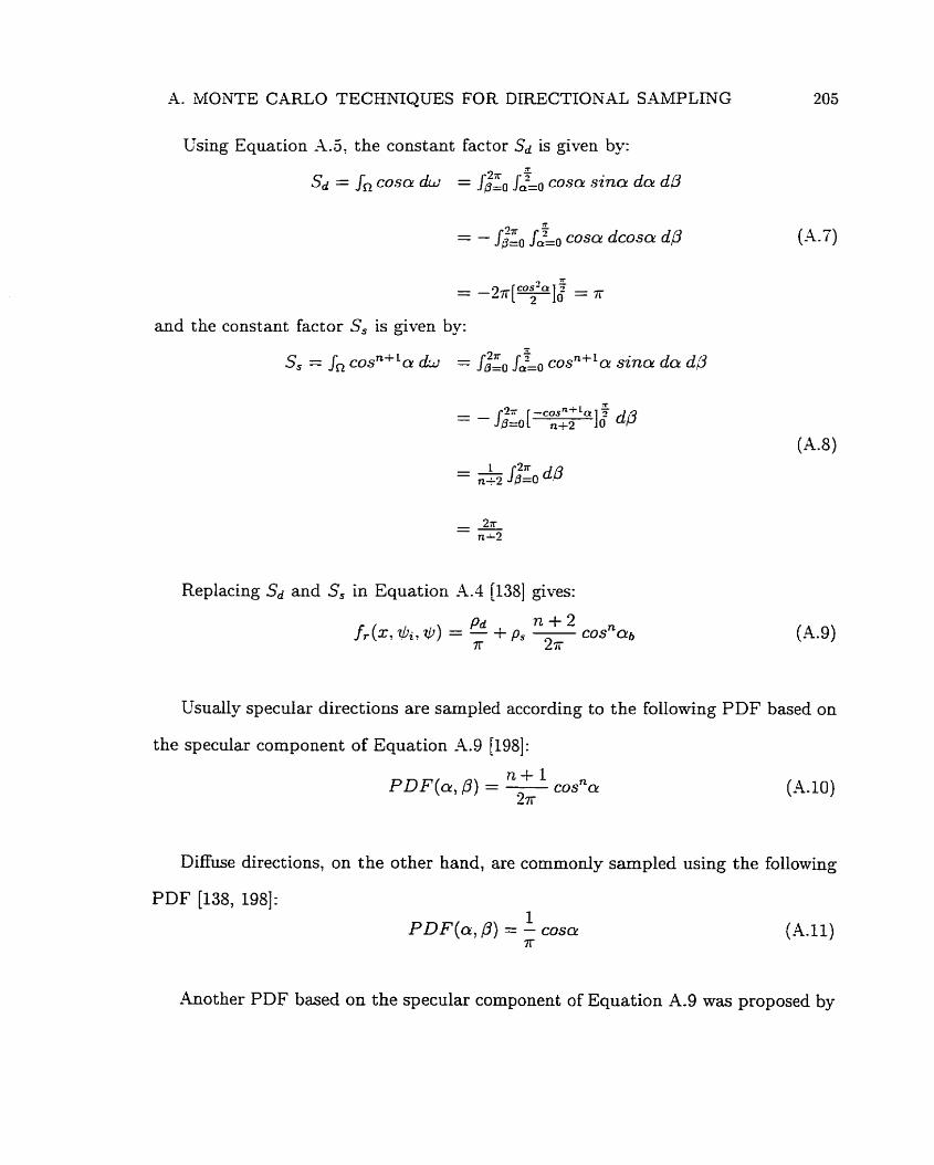
A. MONTE CARLO TECHNIQUES FOR DIRECTTONAL SAMPLING
Using Equation -4.5, the constant factor Sd is given by: - sd = J* COSO. d~ = J~L-, casa sina d a dg
- - - 2 ~ [ ~ ] $ . COS'Q = K
and the constant factor S, is given by:
Replacing Sd and S, in Equation -4.4 [135] gives:
P d n t 2 fr(x7@i7@) = - + p s - C O S ~ Q ( ~
;TT 2.ir
Usually specular directions are sampled according to the following PDF based on
the specular component of Equation A.9 [198]:
Diffuse directions, on the other hand, are commonly sampled using the following
PDF [138, 1981: 1
PDF(a , 0) = - coscu 7r
Another PDF based on the specular component of Equation A.9 was proposed by
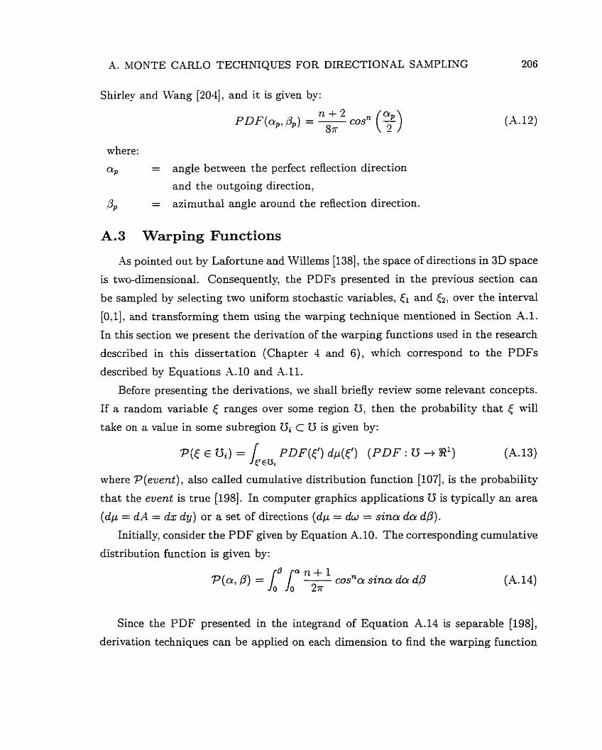
A. MONTE CARLO TECHNIQUES FOR DIRECTIONAL SAMPLING
Shirley and Wang [204], and it is given by:
206
(A. 12)
where:
a~ = angle between the perfect reflection direction and the outgoing direction,
4 = azimuthal angle around the reflection direction.
A. 3 Warping Funct ions
As pointed out by Lafortune and Willems [138], the space of directions in 3D space
is twa-dimensional. Consequently, the PD Fs presented in the previous section can
be sampled by selecting two uniform stochastic variables, El and &; over the interval
[0:1], and transforming them using the warping technique mentioned in Section -4.1.
In this section we present the derivation of the warping functions used in the research
described in this dissertation (Chapter 4 and 6), which correspond to the PDFs
descnbed by Equations A. 10 and A. 11.
Before presenting the derivations, we shall briefly review some relevant concepts.
If a random variable E ranges over some region U, then the probability that E ni11
take on a value in some subregion 0; c U is given by:
where P (euent) , also called cumulative distribution hinction [?07], is the probability
that the event is tme [198]. In computer graphics applications U is typically an area
(dp = d A = dx dy) or a set of directions (dp = dw = sine d a dp).
Initially, consider the PDF given by Equation 4-10. The corresponding cumulative
distribution function is given by:
Since the PDF presented in the integrand of Equation A.14 is separable [198],
derivation techniques can be applied on each dimension to h d the warping function
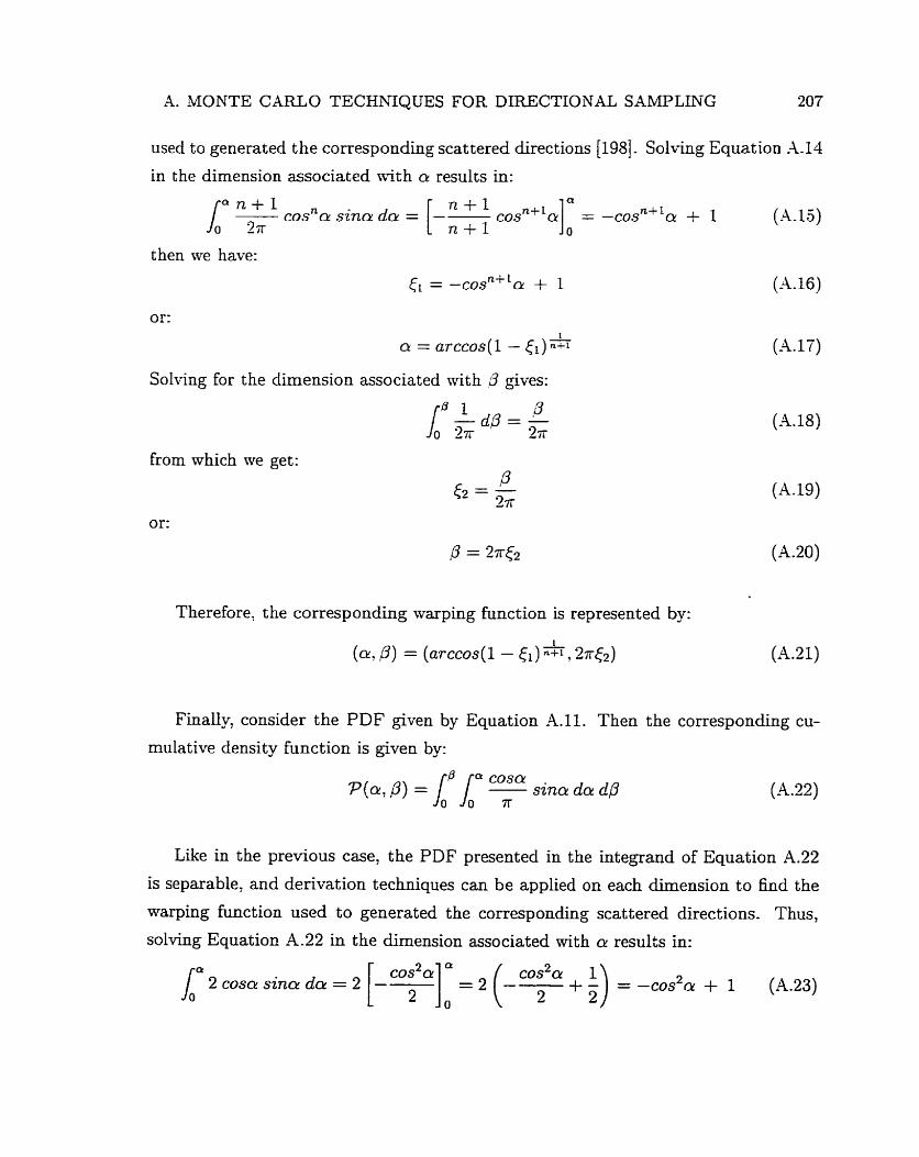
A. MONTE CARLO TECHNIQUES FOR DIRECTIONAL SAMPLIDTG 207
used to generated the corresponding scattered directions 11981. Solving Equation A14
in the dimension associated with a! results in: Q
msnn sinn do = [-"fi casni'c<] = -cosniLa + 1 (-4.15) n t 1 O
then we have:
= -cosn"a + 1
or:
Solving for the dimension associated with B
from which we get:
or:
Therefore, the corresponding warping function is represented by:
(a, ,O) = (arccos(1- cl) *, 27re2) (A.2 1)
Finally, consider the PDF given by Equation A.11. Then the corresponding cu-
mulative density function is given by:
Like in the previous case, the PDF presented in the integrand of Equation A.22
is separable; and derivation techniques can be applied on each dimension to find the
warping function used to generated the corresponding scat tered directions. Thus,
solving Equation A.22 in the dimension associated with a results in:
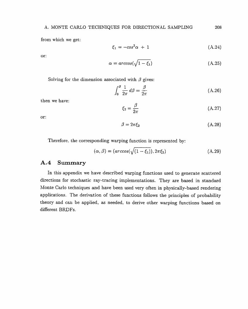
A. MONTE CARLO TECHNIQUES FOR DIRECTIONAL SAMPLING
from which we get:
ci = -cos2a t- 1
or:
Solving for the dimension associated Nith 3 gives:
then we have:
or:
Therefore? the corresponding warping function is represented by :
A.4 Summary
In this appendk we have described warping functions used to generate scattered
directions for stochastic ray-tracing implementations. They are baçed in standard
Monte Car10 techniques and have been used very often in physical-based rendering
applications. The derivation of these hnctions follows the principles of probability
theory and cari be applied, as needed, to derive other warping functions based on
different BRDFs.
APPENDIX B
Accuracy of Wlethods for Form Factor Computation
There are several numerical methods for the computation of form factor between finite
surfaces or patches. In order to select one these methods, speed and accuracy aspects
are taken into account. For off-line computations of form factors, for example aiming
at sun and shade simulations [99] and radiative transfer simulations in vegetation
[48], accuracy becomes the key element since the errors introduced by these methods
affect directly the accuracy of the radiosity solutions (Chapter 7).
Generally speaking, these met hods can be divicied into two groups: deterministic
and nondeterministic. In this appendix we compare the accuracy of two methods
which are representatives of these two groups. With these cornparisons we intend to
highlight some important aspects that affect the accuracy of the numerical methods
for form factor computation. We also intend to discuss the differences in the magni-
tude and in the distribution of the errors associated with the form factors computed
through these two different approaches. The remaining of this appendk is organized
as follon~s:
Section B. 1 outlines the implications of the errors introduced during form factor
computation.
Section B.2 bnefly describes the two methods used in the comparisons.
Section B.3 presents the criteria used to compare the accuracy of these methods.
Section B.4 presents the results of these comparisons.
0 Section B.5 summarizes the main conclusions drawn fkom these comparisons
and suggests directions in which they can be extended.
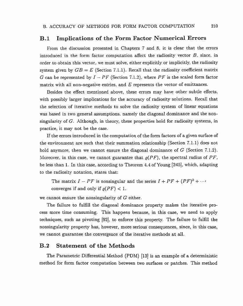
B. ACCUMCY OF METHODS FOR FORA4 FACTOR COMPUTATION 210
B.1 Implications of the Form Factor Numerical Errors
From the discussion presented in Chapters T and 8, it is clear that the errors
introduced in the form factor computation affect the radiosity vector B, since, in
order to obtain this vector, we must solve; either explicitly or implicitly: the radiosity
system given by GB = E (Section 7.1.1). Recall that the radiosity coeEcient matriv
G can be represented by I - PF (Section 7-12). where PF is the scaled form factor
matrix wit h al1 non-negative entries. and E represents the vector of ernittances.
Besides the effect mentioned above, these errors may have other subtle effects,
nrith possibly larger implications for the accuracy of radiosity solutions. Recall that
the selection of iterative rnethods to solve the radiosity system of linear equations
was based in two general assumptions. namely the diagonai dominance and the non-
singularity of G. Although, in theory, these properties hold for radiosity systems. in
practice, it may not be the case.
If the errors introduced in the computation of the form factors of a given surface of
the environment are such that their summation relationship (Section 7.1.1) does not
hold anymore, then we cannot ensure the diagonal dominance of G (Section 7.1.2).
Moreover, in this case, we cannot guarantee that g(PF) , the spectral radius of PF,
be less than 1. In this case, according to Sheorem 4.4 of Young [245], which, adapting
to the radiosity notation, states that:
The matrix 1 - PF is nonsingular and the series 1 + PF + ( P F ) 2 + - . converges if and only if Q(PF) < 1.
we cannot ensure the nonsingularity of G either.
The failure to fulfill the diagonal dominance property makes the iterative pro-
cess more time consuming. This happens because, in this case, we need to apply
techniques, such as pivoting [92], to enforce this property. The failure to fulfill the
nonsingularity property has, however, more serious consequences, since, in this case,
we cannot guarantee the convergence of the iterative methods a t all.
B.2 Statement ofthe Methods
The Parametric Differential Method (PDM) [13] is an example of a deterministic
method for form factor computation between two surfaces or patches. This method
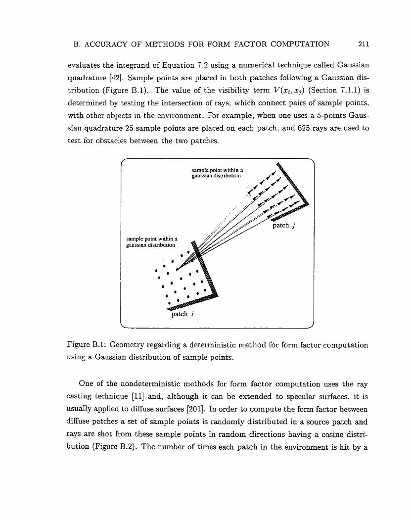
B- ACCUR4CY OF METHOOS FOR FORM FACTOR COWUTATION 211
evaluates the integrand of Equation 7.2 using a numerical technique called Gaussian
quadrature [42]. Sample points are placed in both patches follotving a Gaussian dis-
tribution (Figure B.1). The value of the visibility term V(xi, xj) (Section 7.1.1) is
determined by testing the intersection of rays. which connect pairs of sample points,
mith other objects in the environment. For exarnple, when one uses a 5-points Gaus-
sian quadrature '2s sample points are placed on each patch, and 625 rays are used to
test for obstacles bettveen the two patches.
simple point within a gaussian distribution I 4 /
,/y//5 sample point within ri - 1-7 /
patch i
Figure B.1: Geometry regarding a deterministic met hod for form factor cornputation
using a Gaussian distribution of sample points.
One of the nondeterministic methods for form factor computation uses the ray
casting technique [Il] and, although it can be extended to specular surfaces, it is
usually applied to diffuse surfaces [201]. In order to compute the form factor between
diffuse patches a set of sample points is randornly distributed in a source patch and
rays are shot fkom these sample points in random directions having a cosine distri-
bution (Figure B.2). The number of times each patch in the environment is hit by a
B. ACCURACY OF METHODS FOR FORM FACTOR COMPUTATION
distribution I
patch i A L
4 \ '
Figure B.2: Geometry regarding a nondeterministic method for f o m factor compu-
tation using a random distribution of sample points.
ray is recorded. Then the form factor between a source patch i and a patch j is given
by the number of rays that hit patch j divided by the total number of rays shot from
patch i. Henceforth we will refer to this method as SR, i-e. shooting method with a
random distribution of sample points.
B.3 Cornparison Criteria
In order to evaluate the accuracy of riurnerical methods for form factor compu-
tation it is convenient to use geornetries for which the analytical form factors are
available to be used as reference. In the tests performed in this appendix we con-
sidered an environment formed by a cube, or box (Figure B.3), which allow us to
fulfill this evaluation guideline. Recall that the sumrnation of the form factors of one
surface or patch regarding the other surfaces or patches of a closed environment must
sum to 1 (Section 7.1.1). MTe use this summation relationship as well as the analytical
f o m factors for parallel and perpendicular surfaces to evaluate the accuracy of the
results provided by both methods regarding the test environment.
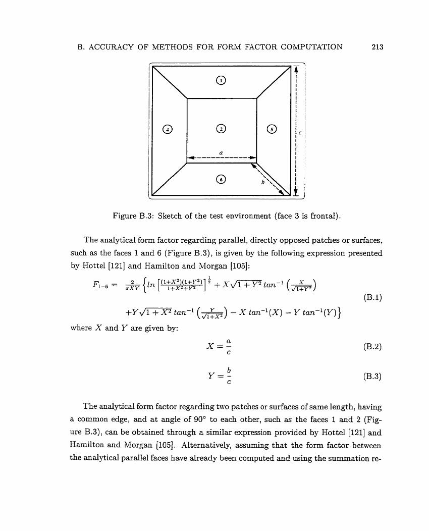
B. ACCUMCY OF METHODS FOR FOR.ii1 FACTOR COMPUTATION 213
Figure B.3: Sketch of the test environment (face 3 is frontal).
The analytical form factor regarding parallel, directly opposed patches or surfaces,
such as the faces 1 and 6 (Figure B.3), is given by the following expression presented
by Hotte1 [El] and Hamilton and Morgan [los]:
+Y J7T-F tan-' (&) - X tan-' (X) - Y tan- '(Y))
where X and Y are given by:
The analytical form factor regarding two patches or surfaces of same length, having
a common edge, and a t angle of 90" to each other, such as the faces 1 and 2 (Fig-
ure B.3), can be obtained through a similar expression provided by Hotte1 [121] and
Hamilton and Morgan (1051. Alternatively, assuming that the form factor between
the analytical parallel faces have already been computed and using the summation re-
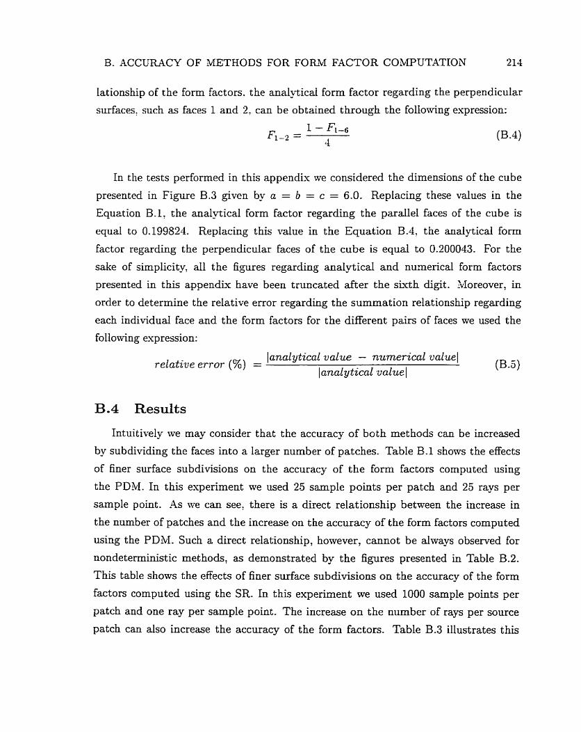
B. ACCURACY OF METHODS FOR FOEtM FACTOR COMPUTATION 214
lat ionship of the form factors. the analytical forrn factor regarding the perpendicular
surfaces! süch as faces 1 and 2, can be obtained through the following expression:
1 - Fl-6 FLd2 =
4 (B-4
In the tests performed in this appendk we considered the dimensions of the cube
presented in Figure B.3 given by a = b = c = 6.0. Replacing these values in the
Equation B.1: the analytical forrn factor regarding the paralle1 faces of the cube is
equal to 0.199824. Replacing this value in the Equation B.4, the analytical form
factor regarding the perpendicular faces of the cube is equal to 0.200043. For the
sake of simplicity, al1 the figures regarding analytical and nurnerical form factors
presented in this appendix have been truncated after the sixth digit. ?vIoreover, in
order to determine the relative error regarding the sumrnation relationship regarding
each individual face and the form factors for the different pairs of faces we used the
following expression:
Janal ytical value - numerical value^ relative error (%) = (B.5)
lanalytical #ualuel
B.4 Results
Intuitively we may consider that the accuracy of both methods can be increased
by subdividing the faces into a larger number of patches. Table E.1 shows the effects
of finer surface subdivisions on the accuracy of the f o m factors computed using
the PDM. In this experiment we used 25 sample points per patch and 25 rays per
sample point. As Ive can see, there is a direct relationship between the increase in
the number of patches and the increase on the accuracy of the form factors computed
using the PDM. Such a direct relationship, however, cannot be always observed for
nondeterministic methods, as demonstrated by the figures presented in TabIe B -2.
This table shows the effects of finer surface subdivisions on the accuracy of the form
factors computed using the SR. In this experiment we used 1000 sample points per
patch and one ray per sample point. The increase on the number of rays per source
patch can also increase the accuracy of the form factors. Table B.3 illustrates this
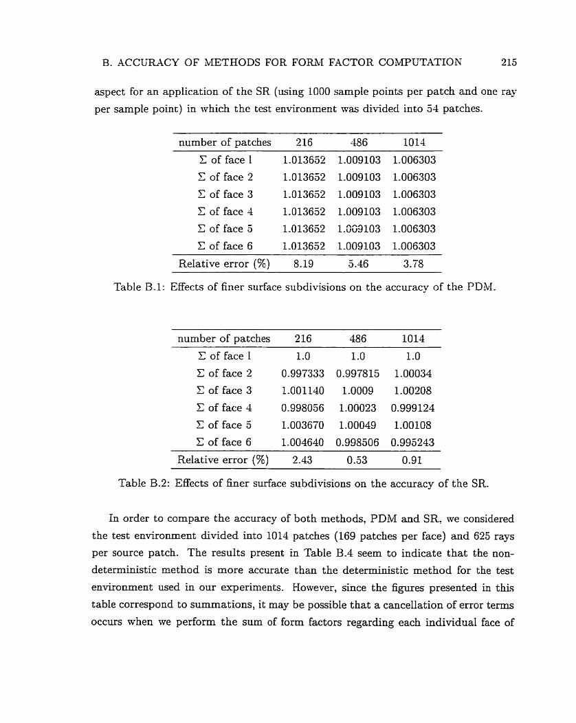
B. ACCURACY OF METHODS FOR FOml FACTOR COMPUTATION 215
aspect for an application of the SR (using 1000 sample points per patch and one ray
per sample point) in mhich the test environment was divïded into 54 patches.
number of patches 216 486 1014
C of face 1 1.013652 1.009103 1.006303
C of face 2 1.013652 1.009103 1.006303
Z of face 3 1.013652 1.009103 1.006303
C of face 4 1-013652 1.009103 1.006303
C of face 5 1.0 13652 1 .ûG3 103 1 .O06303
C of face 6 1-013652 1-009103 1.006303 - -- -- - ---
Relative error (%) 8.19 5.46 3.78
Table B.1: Effects of finer surface subdivisions on the accuracy of the PDM-
number of patches 216 486 1014
C of face 1 1 .O 1 .O 1 .O
C of face 2 0.997333 0.997815 1-00034
C of face 3 1.001140 1.0009 1.00208
C of face 4 0.998056 1.00023 0.999124
C of face 5 1.003670 1.00049 1.00108
C of face 6 1.004640 0.998506 0.995243
Relative error (%) 2.43 0.53 0.91
Table B.2: Effects of finer surface subdivisions on the accuracy of the SR.
In order to compare the accuracy of both methods, PDM and SR, -ive considered
the test environment divided into 1014 patches (169 patches per face) and 625 rays
per source patch. The results present in Table B.4 seem to indicate that the non-
deterministic method is more accurate than the deterministic method for the test
environment used in our experiments. However, since the figures presented in this
table correspond to summations, it may be possible that a cancellation of error terms
occurs when we perform the sum of form factors regarding each individual face of
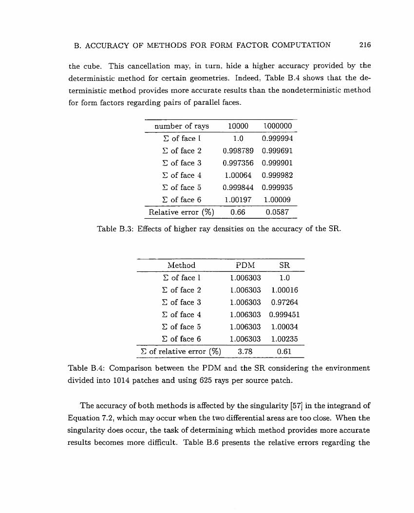
B. ACCURACY OF METHODS FOR FORM FACTOR COMPUTATIOW 216
the cube. This cancellation ma';, in turn. hide a higher accuracy provided by the
deterministic method for certain geometries. Indeed, Table B.4 shows that the de-
terministic met hod provides more accurate results t han the nondeterministic met hod
for form factors regarding pairs of parallel faces.
number of rays 10000 1000000
C of face 1 1 .O 0.999994
C of face 2 0.998739 0.999691
C of face 3 0.997356 0-999901
t of face 4 1 -00064 0-999982
E of face 5 0.999844 0.999935
C of face 6 1.00197 1.00009
Relative error (%) 0.66 0.0587
Table B.3: Effects of higher ray densities on the accuracy of the SR.
C of face 1 1.006303 1.0
C of face 2 1.006303 1.00016
Z of face 3 1.006303 0.97264
C of face 4 1 .O06303 0 -99945 1
C of face 5 1.006303 1.00034
C of face 6 1 -006303 1 .O0235
C of relative error (%) 3.78 0.61 . -. - -
Table B.4: Cornparison between the PDM and the SR considering the environment
divided into 1014 patches and using 625 rays per source patch.
The accuracy of both methods is affected by the singularity [57] in the integrand of
Equation 7.2, which may occur when the two differential areas are too close. When the
singularity does occur, the task of determining which method provides more accurate
results becomes more difficult. Table B.6 presents the relative errors regarding the
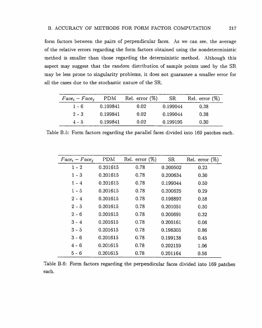
B. ACCURACy OF METHODS FOR FO&M FACTOR COMPUTATION 217
form factors between the pairs of perpendicular faces. As we can see. the average
of the relative errors regarding the form factors obtained using the nondeterminist ic
method is smaller than t hose regarding the deterministic method. Although this
aspect rnay suggest that the random distribution of sample points used b - the SR
may be less prone to singdarity problems, it does not guarantee a smaller error for
al1 the cases due to the stochastic nature of the SR.
Facei - Facej P D M Rel. error (%) SR Rel. error (%)
Table B.5: Form factors regarding the parallel faces divided into 169 patches each.
Facei - Facej P D M Rel. error (%) SR Rel. error (96) 1 - 2 0.201615 0.78 0.200502 0.23
1 - 3 0.201615 0-78 0.200634 0.30
1 - 4 0.201615 0-78 O. 199044 0.50
1 - 5 0.201615 0.78 0.200625 029
2 - 4 0.201615 0.78 0.298892 0.58
2 - 5 0.201615 0.78 0.201051 O .50
2 - 6 0.201615 0.78 0.200691 0.32
3 - 4 0.201615 0.78 0.200161 0.06
Table B.6: Form factors regarding the perpendicular faces divided into 169 patches
each.
B. ACCUMCY OF METHODS FOR FOFW FACTOR COMPUTATION 218
B.5 Summary
In this appendk we have performed comparisons between two numerical methods
for form factor computation based on different approaches. The results of these tests
show that, even for simple environments, such as the one used in our experiments,
a single method cannot provide the nost accurate results for ail possible geornetries.
Lsually, for geometrïes not prone to singularity problems. the deterrninistic met h-
ods may provide more accurate results. Moreover. while the error associated ivith
the deterministic met hods is uniform, the error associated with the nondeterministic
methods is nonuniform. This aspect suggests that statistical anaiysis tools shall be
bring to bear on future comparisons. These comparisons shall take into account more
complex environments, including occlusions and curved objects.
Finally, despite the simplicity of the environment used in our experiments, it
was shown that selecting the "best" method is delicate, since no single method is
superior in al1 cases. The relative accuracy depends on the geometrical characteristics
of the environment. Therefore, developing of accurate practical solutions for off-
line computation of form factors i d 1 likely require implementing different methods,
with the application of a given method determined by the geometry at hand. For
esample, considering the environment used in our experiments, one could use the
deterministic method to compute the form factor regarding the parallel faces and the
nondeterrninistic met hod for the perpendicular faces.
Experiments with Eigenvectors
.lrvo [ï. 91 has shown that several fundamentai operators that arîse in global illumi-
nation c m be uniformly approsimated by matrices. Considering this aspect, if one
can determine what the eigenvectors of a global illumination matrk. like the radiosity
matrix G, represent in terms of the physical application, i t may be possible to obtain
close estimates for these eigenvectors. Shese eigenvectors could, in turn, be used to
obtain low rank approximation of this matrix using single value decomposition (Sm)
type approaches [92].
In some fields the physical meaning of eigenvalues and eigenvectors is well k n o m .
For instance, the eigenvect ors of the stiffness matLu associated with a discretized
structure of uniform density represent the natural modes of vibration of the structure
being studied [195], and the corresponding eigenvalues define the natural frequen-
cies of vibration [143]. In global illumination, however, the physical meaning of the
eigenvalues and eigenvectors is still an open problem.
Although we have shown numericalfy that the distribution of the eigenvalues of
radiosity matrices is affected by increases in the overall reflectance and level of oc-
clusion of the environment (Section 8.6): the physical meaning of the corresponding
eigenvectors has not been addressed yet. In this appendix we show some interesting
features of using eigenvectors of radiosity matrices as solution vectors in graphics
settings in order to contribute to the clarification of this question.
The rernaining sections of this appendix are organized as follows:
Section C.1 describes the experiments set up.
Section C.2 provides the mathematical background for the experiments.
C- EXPERIMENTS WITH EIGENVECTORS 220
Section C.3 presents the experiments regarding the eigenvectors corresponding
to the smallest eigenvalue of the radiosity matrix G.
Section C.4 presents the esceriments regarding the eigenvectors corresponding
to the largest eigenvalue of the radiosity matris G.
Section C.3 presents the experiments regarding the eigenvectors corresponding
to the largest eigenvalue of the symmetrized radiosity mat rix Gs .
Section C.6 presents the experiments regarding the eigenvectors corresponding
to the smallest eigenvalue of the symmetrized radiosity matrix G" .
Finally? Section C.7 summarizes the mains aspects and discusses the practical
implications of the investigation presented in this appendix.
C . 1 Experiments Set-Up
The test scene used in our experiments is described in Section 8.5.2. In this ap-
p e n d i ~ we use two different sets of parameters to allow a wider range of observations.
In set 1 we use one light source corresponding to 16 patches, with an irradiance equal
to 10.0. and we set the reflectance of the sphere to 0.65. In set 2 we use two light
sources, each corresponding to 16 patches, with an irradiance equal to 5.0, and we
set the reflectance of the sphere to 0.55. The reflectances of the light sources are set
to 0.1, and the values assigned for the reflectances of the other surfaces are presented
in Table C.1. The f o m factors are computed using PDM [13]. The eigenvalues and
eigenvectors are computed using MASLAB [154] through the QR method [42] whose
algorit hms are provided by the EISPA CK routines [2 131.
The images presented in this paper are rendered using fiat shading and greyscale
to allow a better detection of the features associated with the eigenvector components.
Figure C.1 shows the images corresponding to the solution (radiosity) vectors of the
radiosity systems of linear equations regarding the two sets of parameters, which
are solved using the Chebyshev method (Section 8.4). These images are used in
our experiments as reference images to be compared with images obtained using
eigenvectors as solution vectors.
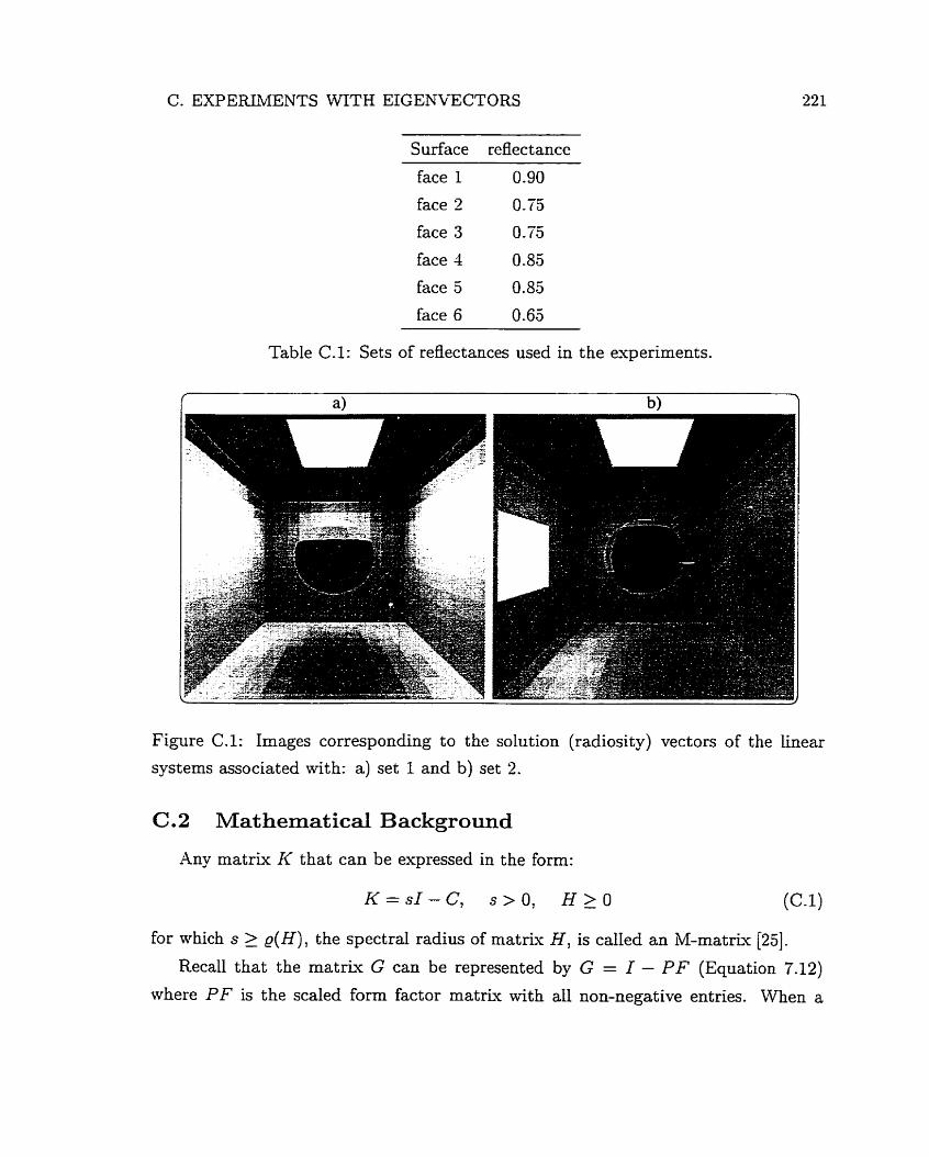
C. EXPERIMENTS WITH EIGENW3CTORS
face 1 0.90
face 2 0.75
face 3 O. 75
face 4 0.85
face 5 0.85
face 6 0.65
Table C.1: Sets of reflectances used in the experiments.
Figure (2.1: Images corresponding to the solution (radiosity) vectors of the linear
systems associated with: a) set 1 and b) set 2.
C .2 Mathematical Background
Any matrix K that can be expressed in the form:
for which s 2 @), the spectral radius of matris H , is called an M-matrk [25].
Recall that the mat& G can be represented by G = I - PF (Equation 7.12)
where PF is the scaled form factor matrk with al1 non-negative entries. When a
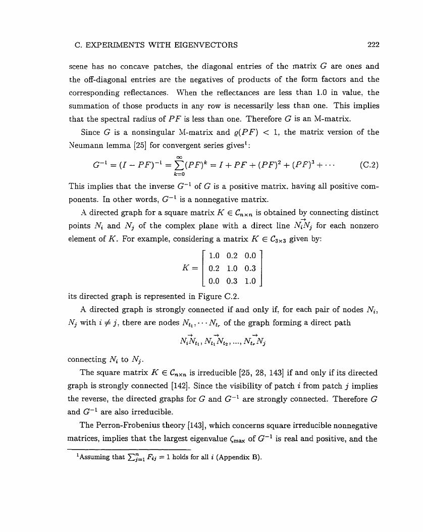
C. EXPERIMENTS WITK EIGENVECTORS 222
scene has no concave patches, the diagonal entries of the rnatriv G are ones and
the off-diagonal entries are the negatives of products of the form factors and the
correspondhg reflectances. When the reflectances are less than 1.0 in value: the
summation of those products in any row is necessarily less than one. This implies
that the spectral radius of PF is less than one. Therefore G is an M-rnatrk.
Since G is a nonsingular M-rnatrix and e (PF) < 1, the matnx version of the
Neumann lemma [23] for convergent series givesL: CO
CL = (1 - P F ) - ~ = ~ ( P F ) ~ = 1 + PF + ( P F ) ~ + (PF)3 + - - - (C.2) k=O
This irnplies that the inverse G-' of G is a positive matriu. having al1 positive com-
pooents. In other words, G-' is a nonnegative ma t rk .
A directed graph for a square matn'c K E C,,, is obtained by connecting distinct +
points lVi and Nj of the complex plane with a direct Line iVilVj for each nonzero
element of K. For example, considering a mat ri^ K E C3x3 given by:
its directed graph is represented in Figure (2.2.
A directed graph is strongly connected if and only if: for each pair of nodes Ni:
iVj with i # j , there are nodes Nt,, - - Nt, of the graph forming a direct path
connecting iVi t0 fVj-
The square matrix K E Cnx, is irreducible [25, 28, 1431 if and only if its directed
graph is strongly connected [142]. Since the visibility of patch i fiom patch j implies
the reverse, the directed graphs for G and G-' are strongly connected. Therefore G
and G-' are d s o irreducible.
The Perron-Frobenius theory (1431, mhich concerns square irreducible nonnegative
matrices, implies that the largest eigenvalue Cm, of G-' is real and positive, and the
'Assuming that x;., Fij = 1 holds for di i (Appendix B).
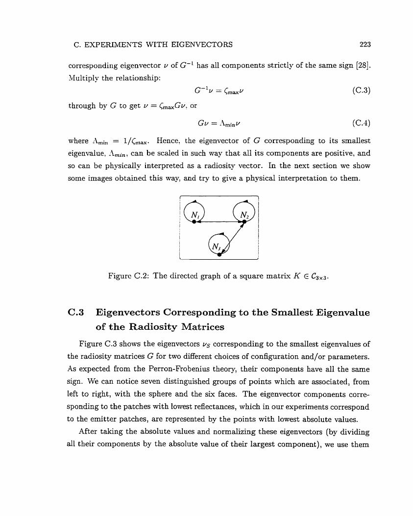
C. EXPERIMENTS WITH EIGENVECTORS 223
corresponding eigenvector u of G-' has al1 cornponents stnctly of the same sign L-81.
Mult iply the relationship:
G-'u = Cmaxu (C-3)
through by G to get v = Cm,Gv: or
where Ami, = l/C,,. Hence. the eigenvector of G corresponding to its smallest
eigenvalue, Ami, can be scaled in such way that al1 its components are positive, and
so can be physically interpreted as a radiosity vector. In the next section we show
sorne images obtained this wax and try to give a physical interpretation to thern.
Figure C.2: The directed graph of a square matKu K E C3x3.
C.3 Eigenvectors Corresponding to the Smallest Eigenvalue
of the Radiosity Matrices
Figure C.3 shows the eigenvectors us corresponding to the smallest eigenvalues of
the radiosity matrices G for two different choices of configuration and/or parameters.
As evpected from the Perron-Frobenius theory, their components have al1 the same
sign. We can notice seven distinguished groups of points which are associated, from
Ieft to right, with the sphere and the six faces. The eigenvector components corre-
sponding to the patches with lowest reflectances, which in our experïments correspond
to the emitter patches, are represented by the points with lowest absolute values.
After taking the absolute values and normalizing these eigenvectors (by dividing
al1 their components by the absolute value of their largest component), we use them
C. EXPERIMENTS WITH EIGENVECTORS 224
as solution vectors to display the images of the scenes (Figure C.4, top row). The
features presented in these images seem to be associated with the distribution of
the reflectances in the scenes (Figure C.4, bottom row). In Figure C.4a we can
notice that the top of the sphere, which is closer to an area with Iow reflectance, is
darker than its bottom. In Figure C.4b. areas of the scene that are directly exposed
to the luminaires are also darker: possibly due to the Iow reflectances assigned to
the emitter patches. These features seem to indicate that the absolute values of
components of the eigenvectors 4 are directly proportional to the refiectance values
of the corresponding patches. F~r the rmore~ they are also associated with the direct
interaction of reflectances. In other words, patches directly exposed to areas with low
reflectance, shown as darker areas in the images, correspond to components of the
eigenvectors Wit h low absolut e values (assuming normalized eigenvectors) .
Figure C.3: Eigenvectors us of the matrices G associated with: a) set 1 and b) set 2.
C .4 Eigenvect ors Corresponding to the Largest Eigenvalue
of the Radiosity Matrices
For the sake of completeness, we also look a t the eigenvector v~ corresponding
to the largest eigenvalue of the radiosity matrices G (Figure C.5). After taking the
absolute values and normalking these eigenvectors, me use them to display the images
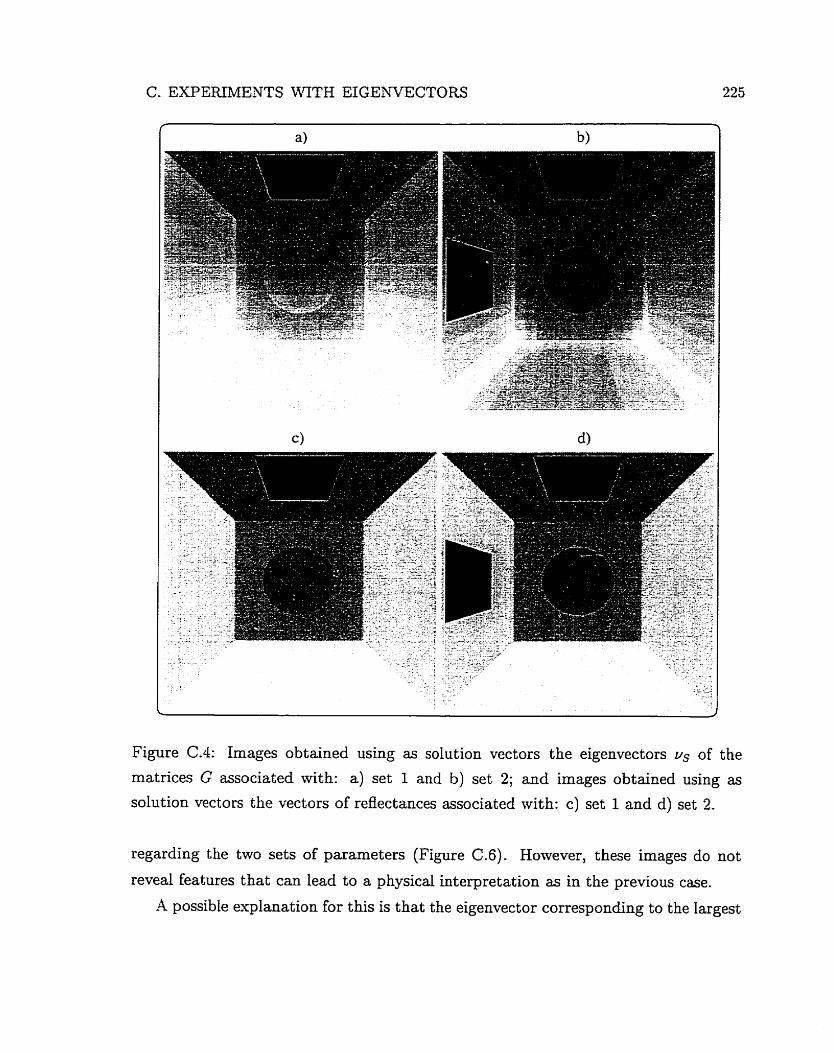
C. EXPERIMENTS WITH EIGENVECTORS
Figure C.4: Images obtained using as solution vectors the eigenvectors us of the
matrices G associated with: a) set 1 and b) set 2; and images obtained using as
solution vectors the vectors of reflectances associated with: c) set 1 and d) set 2.
regarding the two sets of parameters (Figure C.6). However, these images do not
reveal features that can lead to a physical interpretation as in the previous case.
-4 possible evplanation for this is that the eigenvector corresponding to the largest
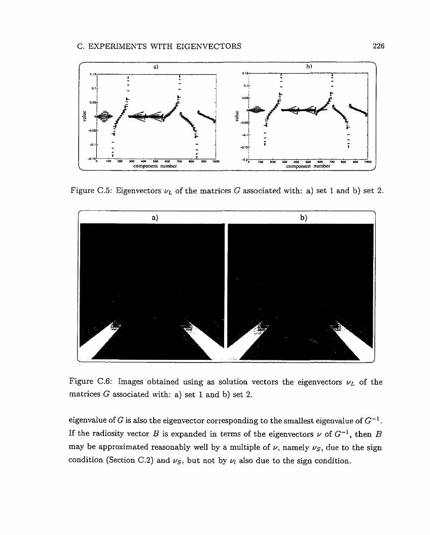
C- EXPERIlh/lENTS WITH EIGENVECTORS 226
Figure (2.5: Eigenvectors v~ of the matrices G associated with: a) set 1 and b) set
Figure C.6: Images obtained using as solution vectors the eigenvectors v~ of the
matrices G associated with: a) set 1 and b) set 2.
eigenvalue of G is also the eigenvector corresponding to the smallest eigenvalue of G-'.
If the radiosity vector B is expanded in terms of the eigenvectors u of G-', then B may be approximated reasonably well by a multiple of u, narnely vs, due to the sign
condition (Section C.2) and US, but not by ul also due to the sign condition.
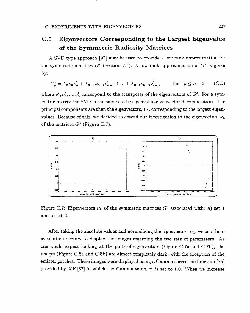
C. EXPERIMENTS WITH EIGENVECTORS
C . 5 Eigenvectors Corresponding to the Largest Eigenvalue
of the Symmetric Radiosity Matrices
-4 SVD type approach [92] may be used to provide a low rank approximation for
the symmetric matrices GS (Section 7.4). A low rank approximation of Gs is given
b y:
Gi = iInvnLn + i \ , - l ~ n - ~ ~ ~ - l + .-. + An-p~n-p~:- , for p $ n - 2 (C.5)
where v;, u;, ..., un correspond to the transposes of the eigenvectors of GS. For a sym-
metric mat rk the SVD is the same as the eigenvalue-eigenvector decornposition. The
principal components are then the eigenvectors, U L , corresponding to the largest eigen-
values. Because of this, we decided to extend our investigation to the eigenvectors u~
of the matrices Gs (Figure C.7).
Figure C.7: Eigenvectors u~ of the symmetric matrices Gs associated with: a) set 1
and b) set 2.
After taking the absolute values and normalizing the eigenvectors u ~ , we use them
as solution vectors to display the images regarding the two sets of parameters. As
one would expect looking a t the plots of eigenvectors (Figure C.7a and C.7b), the
images (Figure C.8a and C.8b) are almost completely dark, with the exception of the
emitter patches. These images were displayed using a Gamma correction function [75]
provided by X V [37] in which the Gamma value, y, is set to 1.0. When we increase
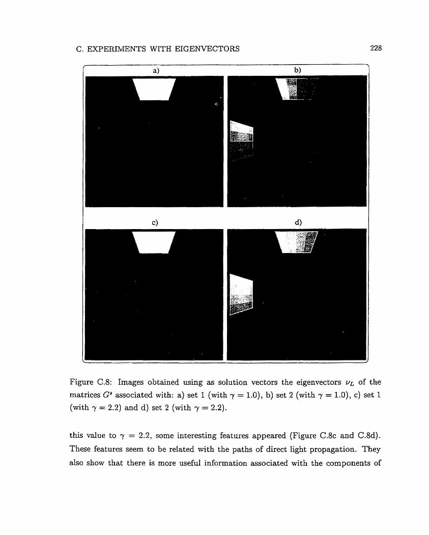
Figure C.8: Images obtained using as solution vectors the eigenvectors UL of the
matrices GS associated with: a) set 1 (with y = 1.0), b) set 2 (with y = 1.0), c) set 1
(with 7 = 2.2) and d) set 2 (with y = 2.2).
this value to y = 2.2, some interesting features appeared (Figure C.8c and C.8d)-
Shese features seem to be related with the paths of direct Light propagation. They
also show that there is more useful information associated with the components of
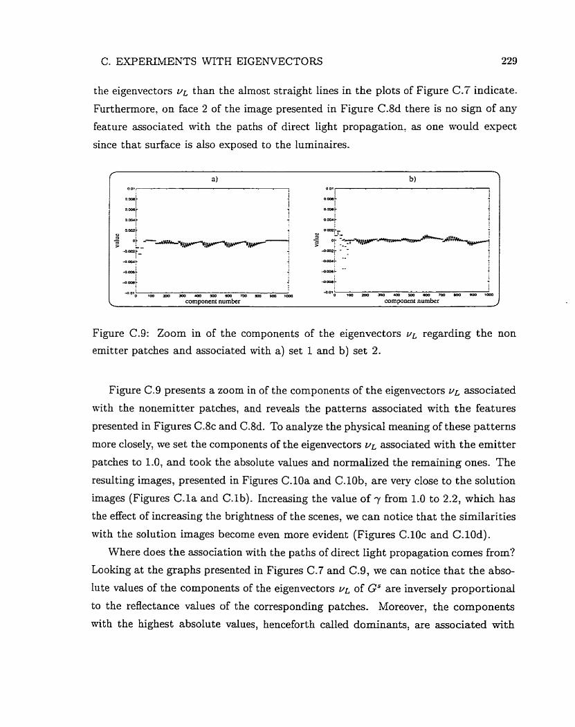
C. EXPERIMENTS WITH EIGENVECTORS 229
the eigenvectors YL than the almost straight lines in the plots of Figure C.7 indicate.
Furthemore, on face 2 of the image presented in Figure C.8d there is no sign of any
feature associated with the paths of direct light propagation, as one would espect
since t hat surface is also exposed to the luminaires.
-0 01 '
O t ~ m o a n ~ m w a m m m m a component nurnber
Figure C.9: Zoom in of the components of the eigenvectors u~ regarding the non
emitter patches and associated with a) set 1 and b) set 2.
Figure C.9 presents a zoom in of the components of the eigenvectors u~ associated
with the nonemitter patches, and reveals the patterns associated with the features
presented in Figures C.8c and C.8d. To analyze the physicai meaning of these patterns
more closely, we set the components of the eigenvectors v~ associated with the emitter
patches to 1.0, and took the absolute values and normalized the remaining ones. The
resulting images, presented in Figures C.lOa and C-lOb, are very close to the solution
images (Figures C - l a and C-l b). Increasing the value of y from 1.0 to 2.2, mhich has
the effect of increasing the brightness of the scenes, we can notice that the similarities
with the solution images become even more evident (Figures C.ZOc and C-lOd).
Where does the association with the paths of direct Light propagation cornes from?
Looking at the graphs presented in Figures C.7 and C.9, we can notice that the abso-
lute values of the components of the eigenvectors v~ of Gs are inversely proportional
to the reflectance values of the corresponding patches. Moreover, the components
wit h the highest absolute values, hencefort h called dominants, are associated with
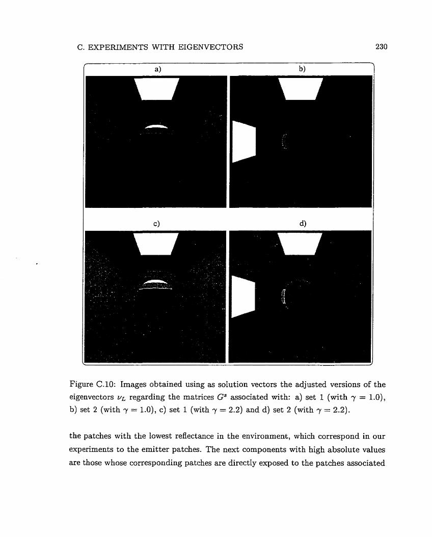
C. EXPERIMENTS WITH EIGENVECTORS
Figure CAO: Images obtained using as solution vectors the adjusted versions of the
eigenvectors v~ regarding the matrices Gs associated with: a) set 1 (with y = 1.0),
b) set 2 (with y = 1.0), c ) set 1 (with y = 2.2) and d) set 2 (with y = 2.2).
the patches with the lowest reflectance in the environment, mhich correspond in our
experiments to the emitter patches. The next components with high absolute values
are t hose whose corresponding pat ches are directly exposed to the pat ches associated
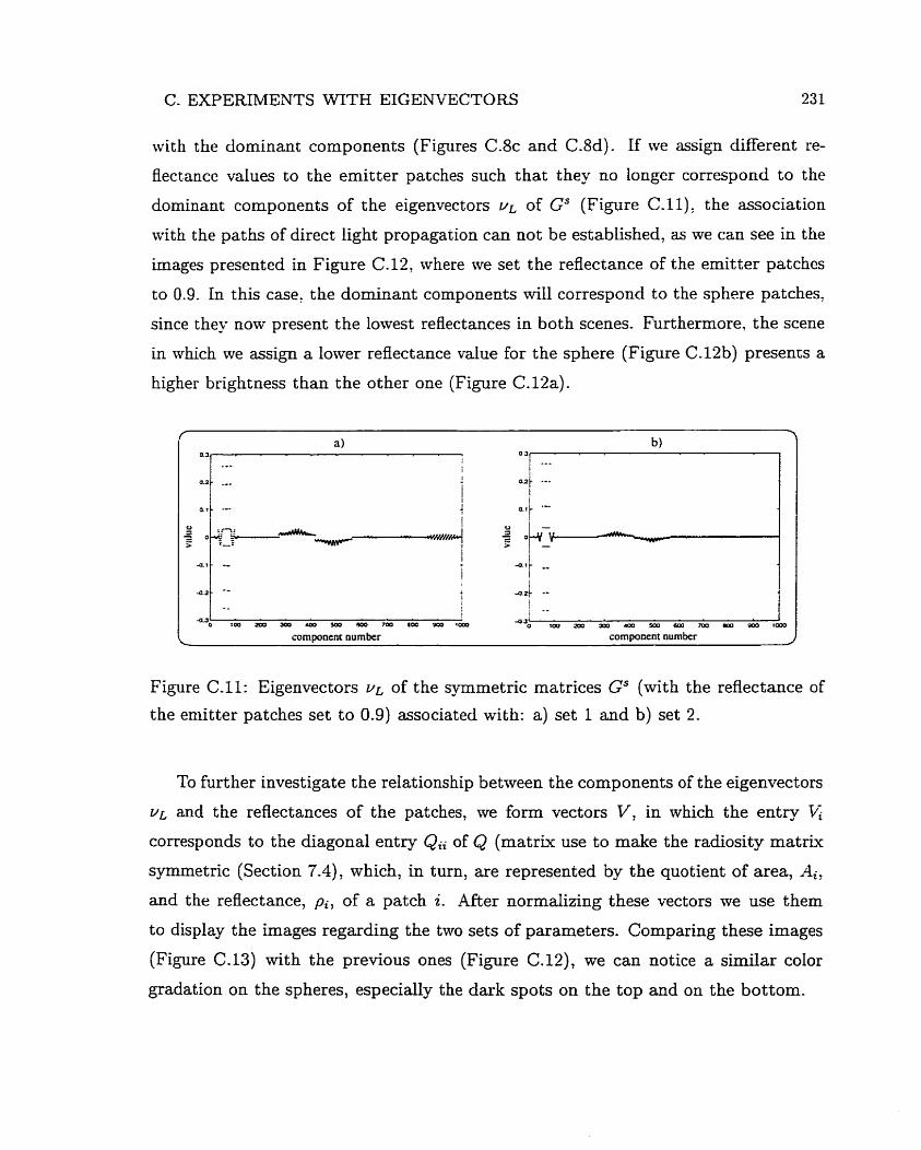
C. EXPERIMENTS WITH EIGENTXCTORS 231
with the dominant components (Figures C.8c and C.8d). If we assign different re-
flectance values to the emitter patches such that they no longer correspond to the
dominant components of the eigenvectors VL of GS (Figure C.11), the association
with the paths of direct light propagation can not be established, as we can see in the
images presented in Figure C.12, where we set the reflectance of the emitter patches
to 0.9. In this case, the dominant components wi11 correspond to the sphere patches,
since they now present the lowest reflectances in both scenes. Furthermore, the scene
in which we assign a lower reflectance value for the sphere (Figure C.12b) presents a
higher brightness than the other one (Figure C. 12a).
4.2 -- - - i
t i
-0 r o o z a > ~ & S m ~ m 1 # : 9 0 0 r a O D
comwnenc number
Figure C.11: Eigenvectors v~ of the symmetric matrices GS (nrith the reflectance of
the emitter patches set to 0.9) associated with: a) set 1 and b) set 2.
To furt her investigate the relationship between the components of the eigenvectors
v~ and the reflectances of the patches, we form vectors V, in which the entry Vi
corresponds to the diagonal entry Qii of Q (matrix use t o make the radiosity m a t r k
symmetric (Section 7.4), which, in turn, are represented 'Dy the quotient of area, Ai,
and the reflectance, pi, of a patch i. After normalizing these vectors we use thern
to display the images regarding the two sets of parameters. Comparing these images
(Figure (2.13) with the previous ones (Figure C.12), we can notice a similar color
gradation on the spheres, especially the dark spots on the top and on the bottom.
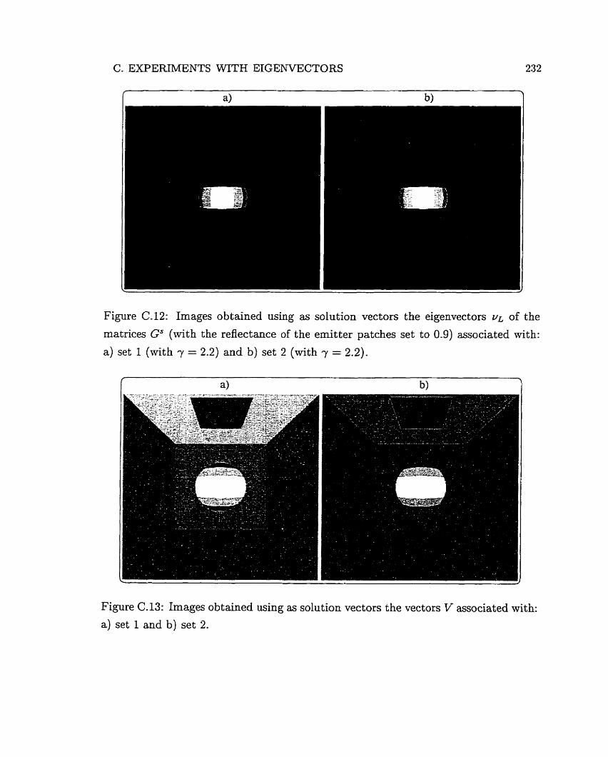
Figure C.12: Images obtained using as solution vectors the eigenvectors v~ of
232
the
matrices Gs (with the reflectance of the emitter patches set to 0.9) associated with:
a) set 1 (with y = 2.2) and b) set 2 (with y = 2.2).
Figure C. 13: Images obtained using as solution vectors the vectors V associated with:
a) set 1 and b) set 2.
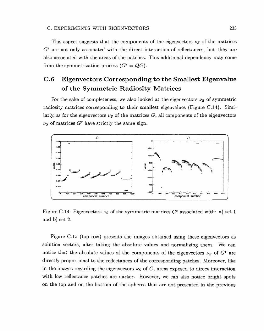
C. EXPERIMENTS WITH EIGENVECTORS 233
This aspect suggests that the components of the eigenvectors us of the matrices
Gs are not only associated with the direct interaction of reflectances, but they are
also associated with the areas of the patches. This additional dependency may corne
from the symmetrization process (Gs = QG).
C.6 Eigenvectors Corresponding to the Smdlest Eigenvalue
of the Symmetric Radiosity Matrices
For the sake of completeness, we also looked at the eigenvectors us of symmetric
radiosity matrices corresponding to their smallest eigenvalues (Figure (2.14). Simi-
larly. as for the eigenvectors us of the matrices G, al1 components of the eigenvectors
us of matrices GS have strictly the same sign.
1
- i
O. . o . , , , , , m m A . ' component number
4.07 . . 1 O m o ~ ~ u I l ~ ~ 7 m a m ~ t m o
cornponent number
Figure C.14: Eigenvectors us of the symmetric matrices Gs associated with: a ) set 1
and b) set 2.
Figure C.15 (top row) presents the images obtained using these eigenvectors as
solution vectors, after taking the absolute values and normalizing them. We can
notice that the absolute values of the cornponents of the eigenvectors us of GS are
directly proportional to the reflectances of the corresponding patches. Moreover, like
in the images regarding the eigenvectors vs of G, areas exposed to direct interaction
with low reflectance patches are darker. However, we can also notice bright spots
on the top and on the bottom of the spheres that are not presented in the previous
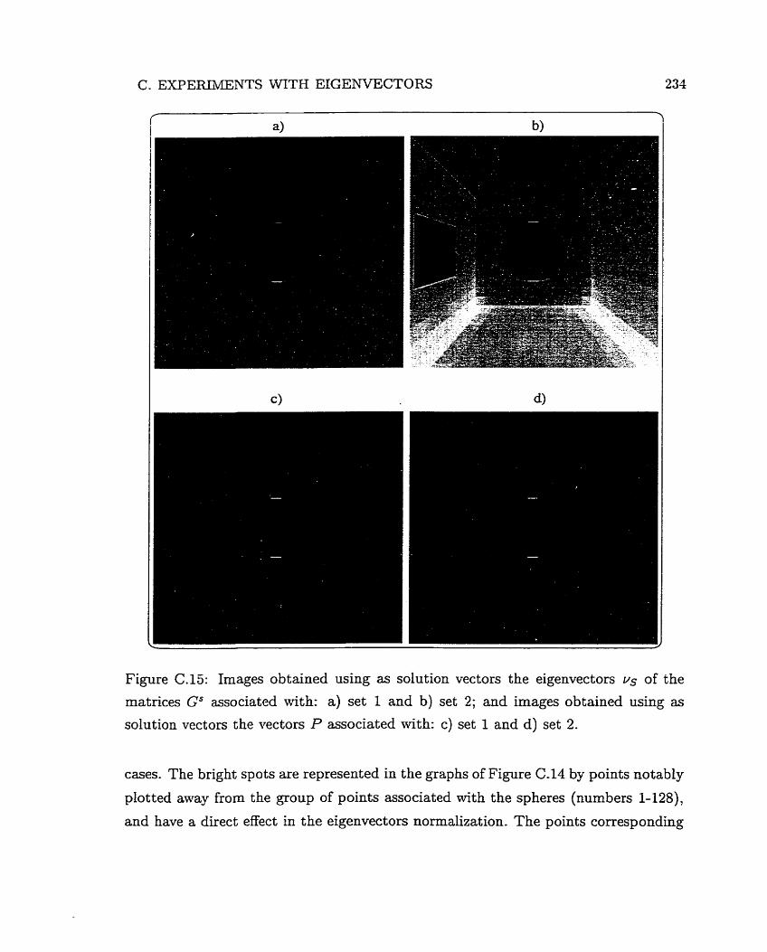
C. EXPERIiLIENTS WITH EIGENVECTORS 234
Figure C.15: Images obtained using as solution vectors the eigenvectors vs of the
matrices Gs associated with: a) set 1 and b) set 2; and images obtained using as
solution vectors the vectors P associated with: c) set 1 and d) set 2.
cases. The bright spots are represented in the graphs of Figure (2.14 by points notably
plotted away frorn the group of points associated with the spheres (numbers 1-128),
and have a direct effect in the eigenvectors normalization. The points corresponding
C- EXPERIMENTS WITH EIGEB'VECTORS 235
to the bright spots associated with set 1 present a higher variance than the points
corresponding to the bright spots associated with set 2. As a result, the image in
Figure C.Ea is considerably darker than the image in Figure C.l5b, despite set 2
having a smaller average reflectance.
To investigate the origin of these bright spots, we compute vectors U , in which the
entry L: corresponds to the inverse of the diagonal entry QG of Q. After normalizing
these vectors we use them to display the images regarding the two sets of parameters.
In these images (Figure 15c and 15d) we can notice the same bright spots. This aspect
suggests that the components of the eigenvectors us of the matrices Gs are not only
associated with the direct interaction of reflectivities, but they are also associated
with the areas of the patches. This additional dependencÿ may also come from the
symmetrizat ion process.
C.7 Discussion and Summary
In this appendk we have shown experiments using eigenvectors of the radiosity
coefficient rnatriv G and its symmetnc version Gs as solution vectors. The compo-
nents of the eigenvectors associated with the srnailest eigenvalue of G have values
directly proportional to the reflectances of the corresponding patches in the scene.
Furthemore, eigenvector components regarding patches evposed to low reflectance
regions have lower absolute values than the remaining components. The components
associated with the largest eigenvalue of GS, however, are inversely proportional to
the reflectances of the corresponding patches. Moreover, for a scene in which the
lowest reflectance values are assigned to the emitter patches, a common procedure
in radiosity applications, this eigenvector provides a very close approximation to the
solution vector. This aspect suggests three possible applications for this eigenvector:
To provide an environment lighting preview for illumination engineering pur-
poses such as selection of luminaires types and locations;
To be used as an initial approximation by iterative methods oriented to the
solution of radiosity systems. We examine this possibility in more detail in the
Appendix D;
C- EXPEFUMENTS WITH EIGENVECTORS
To provide low rank approximations of Gs.
The first two applications mentioned above incorporate the additional overhead
of computing the eigenvalues and eigenvectors. Fortunately. the standard methods
used to determine the eigenvalues and eigenvectors of a matriu? such as the Lanczos
algorithm [64, 921, are themselves iterative. Then, as appropriately noted by DiLaura
and Franck [68] and Ashdown since these methods have the ideal characteristic of
determining the eigenvalues in order of their size: they can be formulated to determine
the largest eigenvalue first and stop the process.
The third application rnentioned above relies on the knowledge of the physical
meaning of eigenvalues and eigenvectors in the radiosity context. With this informa-
tion tve could obtain estimates of the eigenvalues and eigenvectors without having to
explicitly form GS. These estimates could, in turn, be used by SVD type approaches
to obtain a low approximation of Gs, saving both time and memory requirements
for radiosity applications. Unfortunately. the full physical interpretation of radiosity
eigenvalues and eigenvectors remains an open problem. The investigation presented
in t bis appendix, however, provides an experimental substrate for furt her develop
ments in this area, which, as stated by Ashdorvn [IO, 111, remains largely unexplored
in computer graphics despite its significant potential.
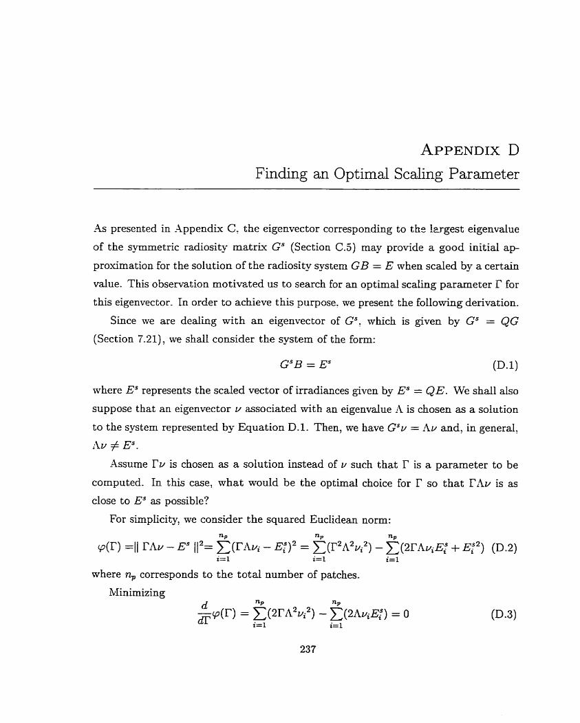
Finding an Optimal Scaling Parameter
As presented in Appendiu CI the eigenvector corresponding to the. lvgest eigenvalue
of the symmetric radiosity rnatrix GS (Section C.3) rnay provide a good initial ap-
proximation for the solution of the radiosity system G B = E when scaled by a certain
value. This observation motivated us to search for an optimal scaling parameter I? for
t his eigenvector. In order to achieve t his purpose. we present the folloiving derivation.
Since we are dealing with an eigenvector of Gs; which is given by GS = QG
(Section 7-21), we s h d consider the system of the form:
where ES represents the scaled vector of irradiances given by ES = QE. We shall also
suppose that an eigenvector v associated with an eigenvalue 12 is chosen as a solution
to the system represented by Equation D.1. Shen, we have GSu = AO and, in general,
Au # ES.
Assume ru is chosen as a solution instead of v such that I' is a parameter to be
cornputed. In this case, what would be the optimal choice for I: so that M u is as
close to ES as possible?
For simplicity, we consider the squared Euclidean norm:
where n, corresponds to the total number of patches.
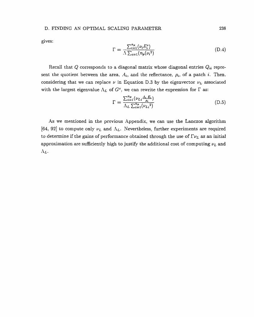
D. FTNDING AN OPTIMAL SCALLVG PARAhETER 238
Recall that Q corresponds to a diagonal matrk whose diagonal entries Qii repre-
sent the quotient between the area. =li, and the reflectance, pi, of a patch i. Then.
considering that me can replace u in Equation D.3 by the eigenvector UL associated
with the largest eigenvalue AL of GS: we can rewrite the expression for as:
As me mentioned in the previous Appendiq we can use the Lanczos algorithm
[64, 921 to cornpute only v~ and AL. Nevertheless, further experiments are required
to determine if the gains of performance obtained through the use of rvL as an initial
approximation are sufficiently high to justify the additional cost of computing u~ and
AL -
Index
abaxial epiderrnist 41
absorptancel 19
absorption spectra, 43
absorptivity, 22
adaxial epidermis, 41
- G R model, 48
ambient term, 124
angiosperms, 45
angle of incidence, 84
anisotropic surface: 33
backscatter, 37
BDF, 19
Beer's law, 22
bifacial leaves, 41
Bouguer's law, 23
BRDF, 19
Brewster's angle, 171
Brewster's law, 171
brightness, 18
BTDF, 19
carotenoids, 43
caustics, 29
characterist ic polynomial, 126
Chebyshev method, 143
chromaticity coordinates, 87
coherent cornponent, 13
color-bleeding, 29
complex index of refraction, 14
conductor, 14
conifers, 43
Conjugate Gradient method, 136
cumulative distribution function, 206
cuticle, 40
density of the radiosity rnatrùi, 118
detour effect, 67
dielec t rics, 14
direct illumination, 4
direct methods, 120
effective absorption coefficient, 65
eigenvalue, 1%
eigenvector, 125
epiticular wax, 40
extinction coefficient, 14
factor of intensification, 67
ferns, 45
form factor, 113
gathering, 122
Gauss-SeideI method, 122
Gaussian elimination, 120
INDEX
general rnatrk methods, 121
geometrical optics, 2
Gerschgorin Circle Theorem, 129
global illumination, 1
glossy surface. 2'7
goniophotometer. 69
gymnosperms, 45
Helmholtz Reciprocity Rule, 20
hemispherical reflectance factor, 69
highlights, 29
hue, 27
importance sampling, 201
incoherent component, 13
indirect illumination, 4
inversion procedure, 47
irreducible matrix, 222
isotropie surface, 32
K-Ad theory, 47
Lambert's cosine law of reflection, 27
Lambert's law of absorption, 22
Lanczos algorithm, 129
law of reflection, 14
law of refraction, 15
light source, 4
light transport, 1
lightness, 27
local illumination rnodel, 5
LOPEX, 65
LU decomposition, 120
luminaire, 4
luminaires, 12
luster: 28
31-matrix: 222
Markov chah , 51
masking effect, 32
matte surface, 27
measurement of appearance, 27
mesophyll, 40
mesophyll lopp, 63
Mie scattering, 44
nonsingular matrix, 129
nonstationary methods, 127
overshooting, 124
palisade cell, 41
Perron-Fro benius theory. 222
photons, 2
physical optics, 3
physically plausible, 20
pigments, 42
plate model, 46
positive definite rnatrix, 128
Power rnethod, 229
preconditioner, 136
probability density function, 202
progressive rehement , 123
Prospect, 47
Pteridophytes, 45
QR factorization, 129
INDEX
quadratic f o r q 137
radiance, 18
radiant energy. 17
radiant in tens i t~ 18
radiant power, 17, 21
radiosity: 116
radiosity linear system, 117
radiosity-specific methods. 12 1
random walk? 59
ray geometrical path length. 64
ray law? 23
Rayleigh scattering, 44
reciprocity relationship, 1 15
reconstruction, 52
refiectance model, B
reflection, 13, 14
reflection haze, 28
refraction, 13
refractive index, 14
refractive-reflect ive scat tering, 44
residual matrix polynomial, 136
residual polynomial, 136
retroreflectance, 37
retroreflection, 37
RMS error, 88
Russian roulette, 78
shooting process, 124
sieve effect, 67
solid angle, 18
spectral condition number, 141
spectral radiant exitance, 114
spectral radiant power, 112
spectral radius, 126
spectrophotorneter, 69
spectrum of a matrix, 125
SPF, 21
spongy cell, 41
stationary methods, 126
Successive Overrelaxation (SOR) , 122
summation relationship, 115
symmetric matrix, 12'7
transmission, 13
trmsmission haze, 28
transparent surface, 27
transpose matriu, 127
unifacial Ieaves, 4 1
venation system, 45
warping, 202
warping functions, 206
SAIL model, 48, 54
saturation, 27
saxpy operation, 154
shadowing effect, 32


![Chapter 2 Selected Topics on Physically-Based Rendering · CHAPTER 2. SELECTED TOPICS ON PHYSICALLY-BASED RENDERING 13 Heckbert [97]: ~t= 2 6 4 i t (~i~n) v u u t1 i t!2 1 (~i~n)2](https://static.fdocuments.in/doc/165x107/60bbcd05bb6f290a92188bfb/chapter-2-selected-topics-on-physically-based-chapter-2-selected-topics-on-physically-based.jpg)