Approximate models for physically based...
45
Approximate models for Physically Based Rendering - Siggraph 2015 Course: Physically Based Shading in Theory and Practice Approximate models for physically based rendering Michał Iwanicki Angelo Pesce Activision
Transcript of Approximate models for physically based...

Approximate models for Physically Based Rendering - Siggraph 2015 Course: Physically Based Shading in Theory and Practice
Approximate models for
physically based rendering
Michał Iwanicki
Angelo Pesce
Activision
Approximate models for Physically Based Rendering - Siggraph 2015 Course: Physically Based Shading in Theory and Practice
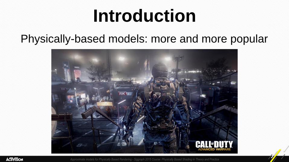
Introduction
Physically-based models: more and more popular

Approximate models for Physically Based Rendering - Siggraph 2015 Course: Physically Based Shading in Theory and Practice
Introduction
• Complex!
– No closed form solutions
– Real time applications can often afford only
the simplest cases
Approximate models for Physically Based Rendering - Siggraph 2015 Course: Physically Based Shading in Theory and Practice
Introduction
• How can we use them in real time?
• Model and approximate!
– Looks just as good (*)
– Way cheaper at runtime
(*) well, ok, almost ;-)
Approximate models for Physically Based Rendering - Siggraph 2015 Course: Physically Based Shading in Theory and Practice
Introduction
• Creating approximate models
– Trial-and-error process
– Practice makes perfect
• Sharing our experience
– Basic guidelines (*)
– Case studies!
(*) No worries, there’s more theory in the course notes
Approximate models for Physically Based Rendering - Siggraph 2015 Course: Physically Based Shading in Theory and Practice
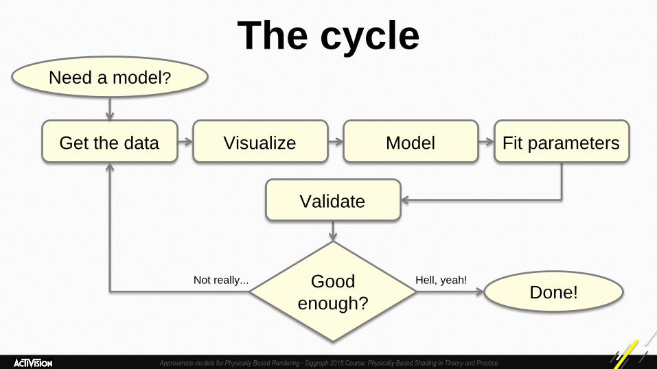
The cycle
Get the data
Not really... Hell, yeah!
Need a model?
Visualize Model Fit parameters
Validate
Good
enough? Done!
Approximate models for Physically Based Rendering - Siggraph 2015 Course: Physically Based Shading in Theory and Practice
1. Acquire the data
• From an existing model:
– E.g. compute the value of the BRDF for every
possible combination of input parameters
– E.g. compute the desired values using costly
precomputations
• From reality:
– Scan/measure
Approximate models for Physically Based Rendering - Siggraph 2015 Course: Physically Based Shading in Theory and Practice
2. Visualize
• Know your enemy, visualize
as much as possible
– Excel, Mathematica, SciPy
– Render cross sections
through different dimensions
– Make visualizations
interactive when possible
Approximate models for Physically Based Rendering - Siggraph 2015 Course: Physically Based Shading in Theory and Practice
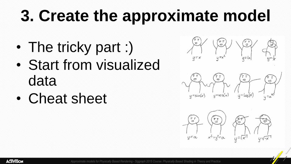
3. Create the approximate model
• The tricky part :)
• Start from visualized data
• Cheat sheet
Approximate models for Physically Based Rendering - Siggraph 2015 Course: Physically Based Shading in Theory and Practice
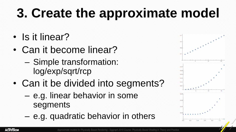
3. Create the approximate model
• Is it linear?
• Can it become linear?
– Simple transformation: log/exp/sqrt/rcp
• Can it be divided into segments?
– e.g. linear behavior in some segments
– e.g. quadratic behavior in others
Approximate models for Physically Based Rendering - Siggraph 2015 Course: Physically Based Shading in Theory and Practice
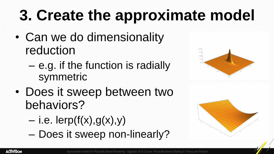
3. Create the approximate model
• Can we do dimensionality reduction
– e.g. if the function is radially symmetric
• Does it sweep between two behaviors?
– i.e. lerp(f(x),g(x),y)
– Does it sweep non-linearly?
Approximate models for Physically Based Rendering - Siggraph 2015 Course: Physically Based Shading in Theory and Practice
3. Create the approximate model
• If nothing simple comes out, try formulating
the model in terms of different variables
– Try combining terms
– Try expressing some terms as combinations
of others
• Careful with the number of free variables!
Approximate models for Physically Based Rendering - Siggraph 2015 Course: Physically Based Shading in Theory and Practice
3. Create the approximate model
• Tools that can create models
automagically exist :
– DEAP, DataModeller, FFX
• But those are only tools
• To paraphrase Mike Abrash:
"the best modelling tool is between your ears”
Approximate models for Physically Based Rendering - Siggraph 2015 Course: Physically Based Shading in Theory and Practice
4. Fit Parameters to your model
• Your model needs parameters
• Optimizer for every occasion:
• Linear regression
• Local: – Gradient descent
– BFGS/L-BFGS
– Levenberg-Marquardt
– E-M
– Nelder-Mead Simplex
• Constrained/unconstrained
• Global: – Differential evolution
– Simulated annealing
– Multistart
Approximate models for Physically Based Rendering - Siggraph 2015 Course: Physically Based Shading in Theory and Practice
5. Check against ground truth
• Check the model in practice, not just on the plots!
• Lowest error doesn’t always mean the best result
– Finding the right metric might be tricky itself!
• Flip between your approximation and reference
• Automate as much as possible
• Collect all results
• Ensure they are reproducible

Approximate models for Physically Based Rendering - Siggraph 2015 Course: Physically Based Shading in Theory and Practice
Time for practice! There’s more in the course notes!
Approximate models for Physically Based Rendering - Siggraph 2015 Course: Physically Based Shading in Theory and Practice
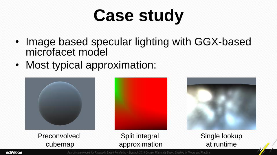
Case study
• Image based specular lighting with GGX-based microfacet model
• Most typical approximation:
Preconvolved
cubemap
Split integral
approximation
Single lookup
at runtime
Approximate models for Physically Based Rendering - Siggraph 2015 Course: Physically Based Shading in Theory and Practice
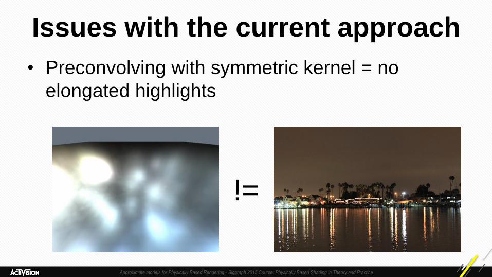
Issues with the current approach
• Preconvolving with symmetric kernel = no
elongated highlights
!=
Approximate models for Physically Based Rendering - Siggraph 2015 Course: Physically Based Shading in Theory and Practice
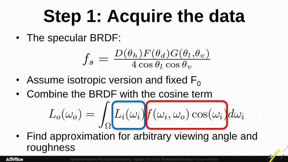
Step 1: Acquire the data • The specular BRDF:
• Assume isotropic version and fixed F0
• Combine the BRDF with the cosine term
• Find approximation for arbitrary viewing angle and roughness
Approximate models for Physically Based Rendering - Siggraph 2015 Course: Physically Based Shading in Theory and Practice
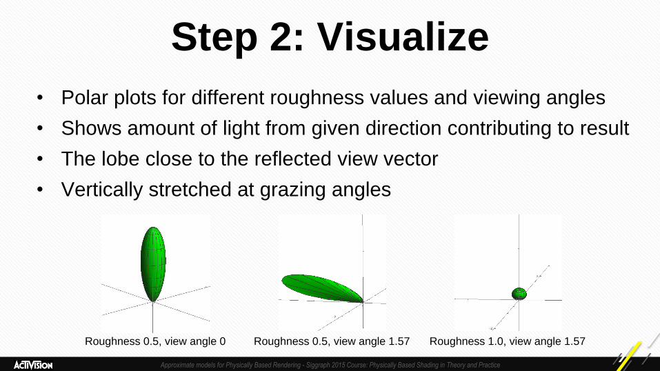
Step 2: Visualize
• Polar plots for different roughness values and viewing angles
• Shows amount of light from given direction contributing to result
• The lobe close to the reflected view vector
• Vertically stretched at grazing angles
Roughness 0.5, view angle 0 Roughness 0.5, view angle 1.57 Roughness 1.0, view angle 1.57
Approximate models for Physically Based Rendering - Siggraph 2015 Course: Physically Based Shading in Theory and Practice
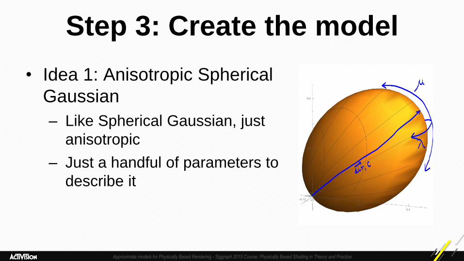
Step 3: Create the model
• Idea 1: Anisotropic Spherical
Gaussian
– Like Spherical Gaussian, just
anisotropic
– Just a handful of parameters to
describe it
Approximate models for Physically Based Rendering - Siggraph 2015 Course: Physically Based Shading in Theory and Practice
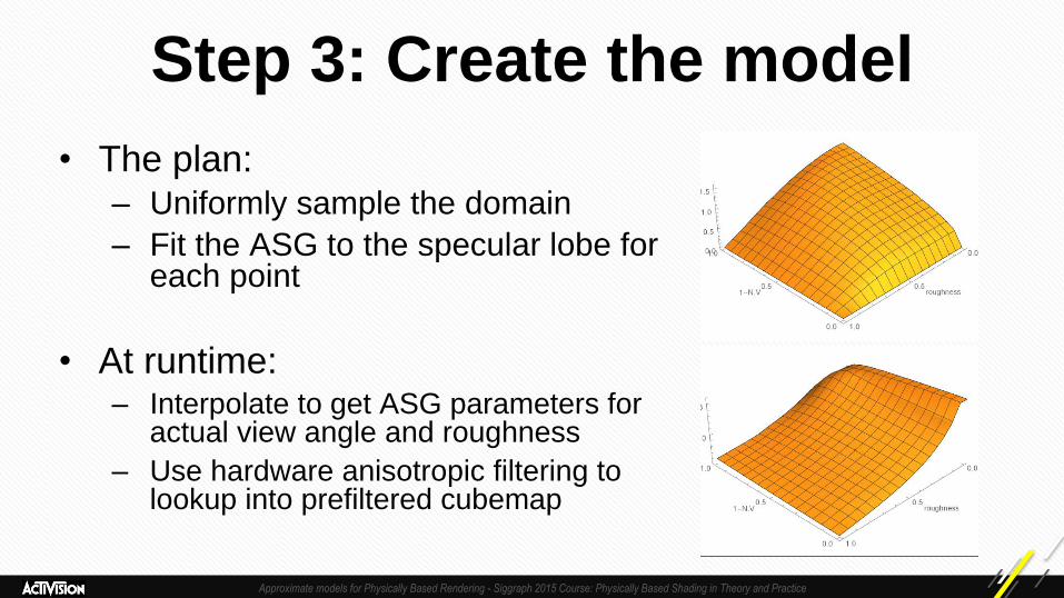
Step 3: Create the model
• The plan: – Uniformly sample the domain
– Fit the ASG to the specular lobe for each point
• At runtime: – Interpolate to get ASG parameters for
actual view angle and roughness
– Use hardware anisotropic filtering to lookup into prefiltered cubemap
Approximate models for Physically Based Rendering - Siggraph 2015 Course: Physically Based Shading in Theory and Practice
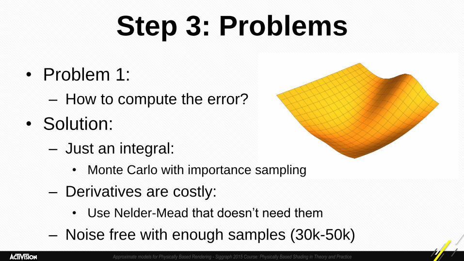
Step 3: Problems
• Problem 1:
– How to compute the error?
• Solution:
– Just an integral:
• Monte Carlo with importance sampling
– Derivatives are costly:
• Use Nelder-Mead that doesn’t need them
– Noise free with enough samples (30k-50k)
Approximate models for Physically Based Rendering - Siggraph 2015 Course: Physically Based Shading in Theory and Practice
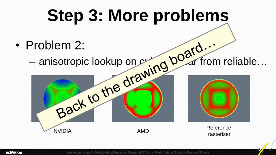
Step 3: More problems
• Problem 2:
– anisotropic lookup on cubemap far from reliable…
NVIDIA AMD Reference
rasterizer
Approximate models for Physically Based Rendering - Siggraph 2015 Course: Physically Based Shading in Theory and Practice
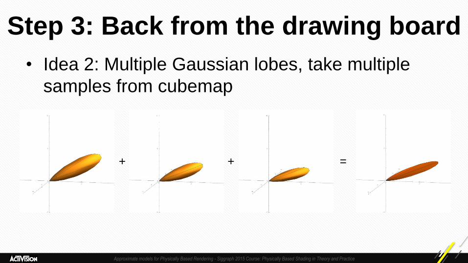
Step 3: Back from the drawing board
• Idea 2: Multiple Gaussian lobes, take multiple
samples from cubemap
+ + =
Approximate models for Physically Based Rendering - Siggraph 2015 Course: Physically Based Shading in Theory and Practice
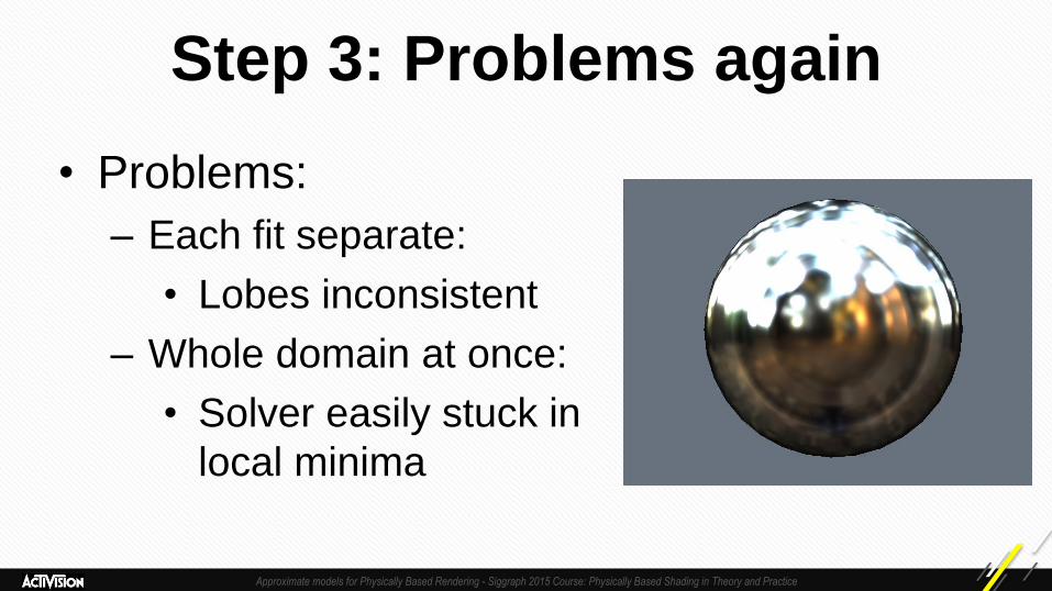
Step 3: Problems again
• Problems:
– Each fit separate:
• Lobes inconsistent
– Whole domain at once:
• Solver easily stuck in
local minima
Approximate models for Physically Based Rendering - Siggraph 2015 Course: Physically Based Shading in Theory and Practice
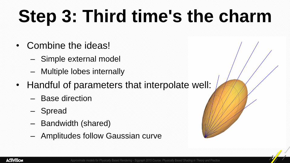
• Combine the ideas!
– Simple external model
– Multiple lobes internally
• Handful of parameters that interpolate well:
– Base direction
– Spread
– Bandwidth (shared)
– Amplitudes follow Gaussian curve
Step 3: Third time's the charm
Approximate models for Physically Based Rendering - Siggraph 2015 Course: Physically Based Shading in Theory and Practice
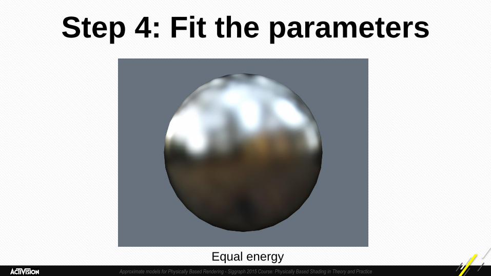
Step 4: Fit the parameters
• Nelder-Mead fit for every view angle and
roughness combination
• Local algorithm – it needs a good starting point:
– Generate near the expected solution
– Scan the domain and pick points with low error
Approximate models for Physically Based Rendering - Siggraph 2015 Course: Physically Based Shading in Theory and Practice
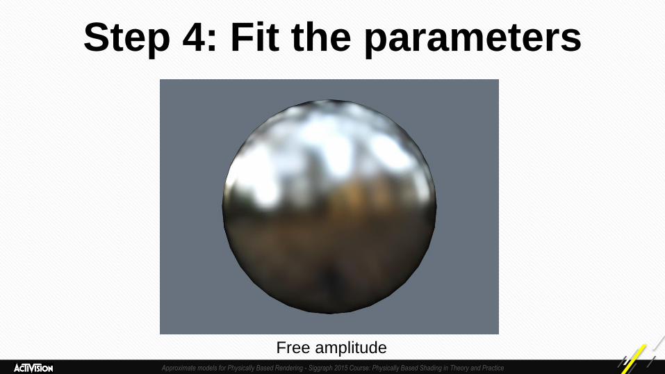
Step 4: Fit the parameters
• Fit values for roughness x view angle domain
– Each data point independent
– Each starting point independent
• Parallelize!
• Two variants:
– Amplitude forced to generate equal energy as GGX
– Amplitude as free variable
Approximate models for Physically Based Rendering - Siggraph 2015 Course: Physically Based Shading in Theory and Practice
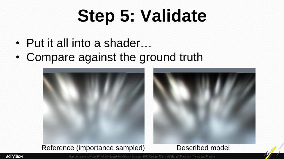
Step 5: Validate
• Put it all into a shader…
• Compare against the ground truth
Reference (importance sampled) Described model
Approximate models for Physically Based Rendering - Siggraph 2015 Course: Physically Based Shading in Theory and Practice
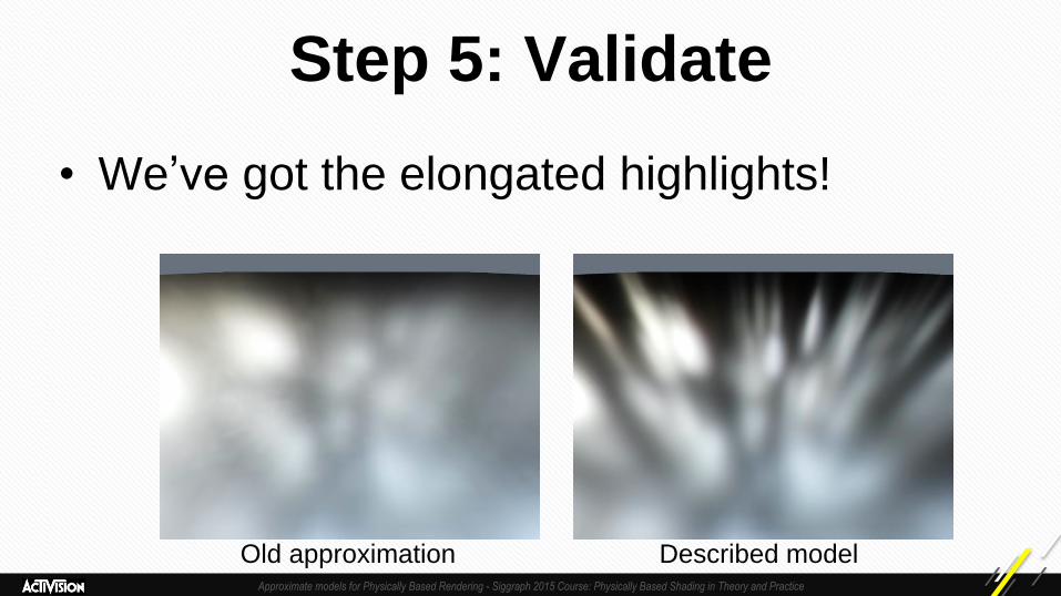
Step 5: Validate
• We’ve got the elongated highlights!
Old approximation Described model
Approximate models for Physically Based Rendering - Siggraph 2015 Course: Physically Based Shading in Theory and Practice
Step 4: Fit the parameters
Equal energy
Approximate models for Physically Based Rendering - Siggraph 2015 Course: Physically Based Shading in Theory and Practice
Step 4: Fit the parameters
Free amplitude

Approximate models for Physically Based Rendering - Siggraph 2015 Course: Physically Based Shading in Theory and Practice
Step 5: Validate more
• What happens at high
roughness?
• When spread > θ we
get radial artifacts
• Damn, so close...
Approximate models for Physically Based Rendering - Siggraph 2015 Course: Physically Based Shading in Theory and Practice
Corrections to the model
• Add a constraint, make sure that spread is no
larger than θ
• Super simple with Nelder-Mead:
– Penalty term
– Trivial changes to the algorithm itself
• Not entirely kosher, but works just fine in practice

Approximate models for Physically Based Rendering - Siggraph 2015 Course: Physically Based Shading in Theory and Practice
Step 5.1: Validate again
• Much better
Approximate models for Physically Based Rendering - Siggraph 2015 Course: Physically Based Shading in Theory and Practice
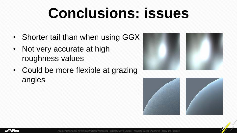
Conclusions: issues
• Shorter tail than when using GGX
• Not very accurate at high
roughness values
• Could be more flexible at grazing
angles
Approximate models for Physically Based Rendering - Siggraph 2015 Course: Physically Based Shading in Theory and Practice
Conclusions
• What’s next?
– Different number of lobes for different parts of the
domain
– Anisotropic BRDFs
– Combine with frequency-based normal map filtering
for shader antialiasing

Approximate models for Physically Based Rendering - Siggraph 2015 Course: Physically Based Shading in Theory and Practice
More in the course notes! Much, much more!
Approximate models for Physically Based Rendering - Siggraph 2015 Course: Physically Based Shading in Theory and Practice
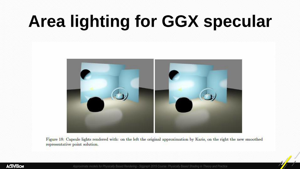
Area lighting for GGX specular
Approximate models for Physically Based Rendering - Siggraph 2015 Course: Physically Based Shading in Theory and Practice
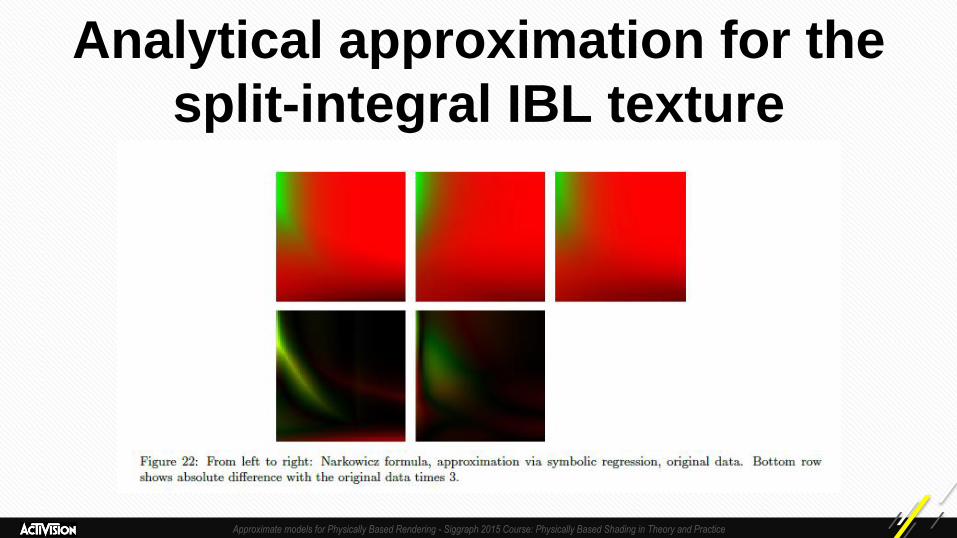
Analytical approximation for the
split-integral IBL texture
Approximate models for Physically Based Rendering - Siggraph 2015 Course: Physically Based Shading in Theory and Practice
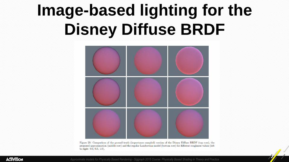
Image-based lighting for the
Disney Diffuse BRDF
Approximate models for Physically Based Rendering - Siggraph 2015 Course: Physically Based Shading in Theory and Practice
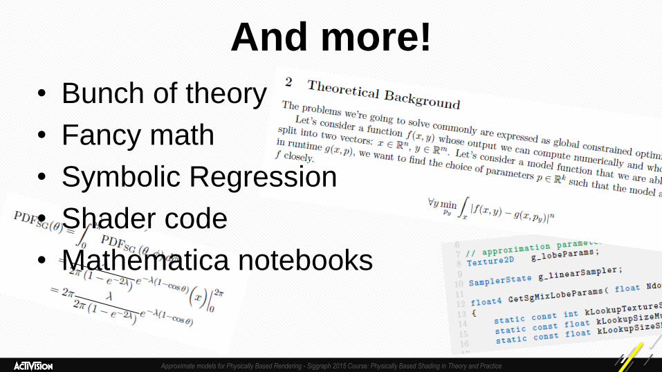
And more!
• Bunch of theory
• Fancy math
• Symbolic Regression
• Shader code
• Mathematica notebooks

Approximate models for Physically Based Rendering - Siggraph 2015 Course: Physically Based Shading in Theory and Practice
Acknowledgments
• Steve Hill, Steve McAuley
• All the smart people we work with, including but
not limited to:
• Peter-Pike Sloan
• Joe Manson
• Mike Stark
• Paul Edelstein
• Jorge Jimenez
• Danny Chan
• Dave Blizard
• Demetrius Leal
• Dimitar Lazarov

Approximate models for Physically Based Rendering - Siggraph 2015 Course: Physically Based Shading in Theory and Practice
Q&A
Contact us (we mean it): [email protected]
[email protected], @kenpex