Comput MechDOI 10.1007/s00466-009-0407-2

ORIGINAL PAPER

Bergström–Boyce model for nonlinear finite rubber viscoelasticity:theoretical aspects and algorithmic treatment for the FE method

Hüsnü Dal · Michael Kaliske

Received: 2 September 2008 / Accepted: 30 June 2009© Springer-Verlag 2009

Abstract One of the successful approaches to model thetime-dependent behaviour of elastomers is proposed byBergström and Boyce (JMPS 46:931–954, 1998). The modelis micromechanically inspired from the relaxation of a singleentangled chain in a polymer gel matrix. Although the the-ory of inelasticity based on multiplicative decomposition ofthe deformation gradient is well established, the complexityof the nonlinear evolution law as well as the nonlinear equi-librium and non-equilibrium material response necessitatesa precise description of the algorithmic setting. This contri-bution presents for the first time a novel numerical imple-mentation of the Bergström–Boyce model in the context offinite element analysis and elaborates theoretical aspects ofthe model. The thermodynamical consistency of the evolu-tion law is proven and a parameter study with respect to thematerial parameters has been carried out. The agreement ofthe model with the recent experimental data is investigated.

Keywords Finite viscoelasticity · Rubber viscoelasticity ·Hysteresis · Algorithmic setting · Thermodynamicalconsistency

1 Introduction

Rubbery polymers exhibit both elastic and viscous mate-rial behaviour simultaneously. The non-equilibrium responseof rubbery polymers attracted many scientists from appliedphysics, material science and engineering. Since elastomericmaterials constitute a great part in industry, the importanceof precise analysis and design necessitates the incorporationof highly sophisticated material models in simulation tools.

H. Dal ·M. Kaliske (B)Institute for Structural Analysis, Technische Universität Dresden,01062 Dresden, Germanye-mail: michael.kaliske@tu-dresden.de

One of the recent attempts for the description of rate-depen-dent material behaviour of rubbery polymers is made byBergström and Boyce [1]. In the contribution on hand,theoretical and numerical aspects of the Bergström andBoyce model (BB model) will be discussed. It will be shownthat the proposed evolution law is a more general repre-sentation of the finite viscoelasticity model of Reese andGovindjee [2], with slight differences. Reese and Govindjee[2] proposed an evolution law which, when linearized aroundthe thermodynamic equilibrium, yields the finite linear vis-coelasticity model of Lubliner [3]. Ignoring the volumetricviscosity term in the finite viscoelasticity model and extend-ing the materially linear evolution of Reese and Govindjee[2], one obtains a more general expression for finite visco-elasticity as proposed by Bergström and Boyce [1]. It willbe further demonstrated that the algorithmic implementa-tion of the model can be done similarly to the algorithmproposed by Simo and Miehe [4] for finite elastoplasticityand by Simo [5] for viscoplasticity. Integration of the evo-lution law will be carried out by an exponential mappingalgorithm (see Weber and Anand [6], Cuitino and Ortiz [7]).Such an approach has been adopted to finite viscoelasticityby Reese and Govindjee [2]. With slight modifications, thesame algorithmic structure can be restructured for the BBmodel. The finite viscoelasticity model proposed by Reeseand Govindjee [2] is constructed on the Ogden type materialmodels (see Ogden [8]). However, the algorithm proposed in[2] covers a general framework of viscoelasticity based ona multiplicative split of deformation gradient and an evolu-tion law as a function of elastic left Cauchy-Green tensor be.The evolution law proposed has a simple linear form whichincludes a constant volumetric and isochoric viscosity terms.The evolution law of the BB model includes invariants ofthe inelastic right Cauchy-Green tensor C i which spoils thesimple representation in terms of principal stretches of be.

123

Comput Mech

Recently, Areias and Matous [9] developed a new finite ele-ment formulation for viscoelastic materials and employedthe method for the BB model. The evolution law is rewrittenin a Lagrangean setting in terms of rate of C i . The resid-ual expression stemming from the evolution law is updatedfor C i and �γ . We will extend the algorithmic approachadopted by Reese and Govindjee [2] for the implementationof the BB model within a distinct framework of volumetric-isochoric split of the free energy density. Within this context,the generalized stresses and the moduli expressions neces-sary for standard and mixed Jacobian-pressure finite elementformulation (Q1/P0 element) will be derived. The advantageof the proposed formulation over the formulation of Areiasand Matous [9] is that inversion operations involve only 3×3matrices with 3 unknowns in the eigenspace of be, whereasthe latter formulation involves lengthy operations with tensorinversions. However, this is done at the expense of accuracyof the algorithm since the invariant terms of C i in the evo-lution law are a priori assumed to be constant and updatedfrom the history variables for a given time step.

1.1 Constitutive approaches to rubber elasticityand viscoelasticity

Many material models for the description of the elastic andviscous behaviour of rubber exist. The accuracy of a proposedviscoelasticity model depends not only on the performanceof the constitutive law for the evolution of the internal vari-able, but also on the constitutive model describing the groundstate elastic response. Recently, Marckmann and Verron [10]discussed 21 rubber elasticity models and compared the per-formance of the formulations with respect to the fitting capa-bilities to uniaxial tension, equibiaxial tension and pure sheardata from Treloar [11] and Kawabata et al. [12], according tothe fitting capability up to stretch level of 400% at which theisoprene rubber shows a reversible elastic behaviour with-out crystallization. The extended tube model of Kaliske andHeinrich [13], the micro-sphere model of Miehe et al. [14]and the Ogden model are cited as the most successful modelsamong others. The Ogden model depends on a phenomeno-logical description of the free energy function and the modelparameters do not have any physical interpretation. The suc-cess of the extended tube model and the micro-sphere modeldepends on the incorporation of tube like constraints whichtake into account the restrictions on the motion of a freechain due to the chains in the neighbourhood or the so-calledforest chains. Additional to a tube constraint part, the micro-sphere model depends on an average network stretch whichis linked to the macro-continuum stretches via p-root aver-aging of the macro stretches in discrete orientation direc-tions. The BB model uses the 8-chain model of Arruda andBoyce [15] for the ground state elastic response and for theMaxwell branch of the model. The 8-chain model provides

quite satisfactory results for uniaxial data, however, underes-timates the equi-biaxial and pure shear response at moderateand large deformations due to the fixed relationship betweenlocking stretches for different deformation modes. On theother hand, considering that the model depends only on twomaterial parameters, it yields quite satisfactory results and thesimplicity of the parameter identification makes the modelpopular for industrial applications.

Two molecular approaches for the description of thetime-dependent behaviour of polymers exist. Transient net-work theory explains the stress relaxation phenomenon as aconsequence of breakage and reformation of the cross-linksconstantly. The theory is firstly proposed by Green andTobolsky [16] and further developed by Lodge [17], Phan-Thien [18] and Tanaka and Edwards [19,20]. Reptation-typetube models are developed for the definition of the motionof a single chain in a polymer gel. The constraints on thefree motion of a single chain are qualitatively modeled as atube-like constraint and the motion of the chain is describedas a combination of Brownian motion within and reptation-al motion along the tube. The model is proposed by DeGennes [21] and Doi and Edwards [22]. The reptationalmotion is successfully adopted to finite viscoelasticity byBergström and Boyce [1]. Recently, Miehe and Göktepe [23]proposed a finite viscoelasticity model depending on twomicro-kinematic scalar internal variables on discrete spaceorientations of the micro-sphere. They propose two micro-mechanisms for the relaxation process of polymer chains:The relaxation of superimposed entanglements and therelease of topological constraints is taken into account bya spectrum of nonlinear evolution laws in the logarithmicspace of the discrete space orientations.

The paper is organized as follows: In Sect. 2, the basicequations governing finite viscoelasticity and the thermo-dynamics in terms of the concept of dissipation are intro-duced. Section 3 presents a complete algorithmic setting forthe Bergström–Boyce model suitable for large strain finiteelement analysis. In Sect. 4, the efficiency of the model isvalidated with a benchmark example and a parameter studywith respect to material parameters is carried out. Finally,concluding remarks close the paper.

2 Continuum mechanical basis of viscoelasticity

Let ϕ : X �→ x be the deformation map at time t ∈R+ ofa body. ϕ maps points X ∈ B of the reference configura-tion B ⊂ R3 onto points x = ϕ(X; t) ∈ S of the currentconfigurationS ⊂ R3. Let F := ∇ϕ(X; t) denote the defor-mation gradient with the determinant J := det F > 0. Thematerial time derivative of the deformation gradient F = lFwhere l := ∇v is the spatial velocity gradient. The bound-ary-value problem for a general inelastic body is governedby the balance of momentum

123

Comput Mech

ρ0 ϕ = div[τ/J ] + γ (1)

along with prescribed displacement boundary conditionsϕ =ϕ(X; t) on ∂Bt and traction boundary conditions [τ/J ]n =t with outward normal n. ρ0 is the density and γ is the pre-scribed body force with respect to unit volume of the currentconfiguration. Let furthermore g = δab denote the covariantCartesian metric tensor or the so-called Kronecker symbolin the current configuration. Due to nearly incompressiblebehaviour of elastomers, we will consider the split of theelastic response into the volumetric and isochoric parts andthe viscous effects are assumed to be purely isochoric

F := J−1/3 F. (2)

The unimodular part of the deformation gradient is furthersplit into elastic and inelastic contributions

F = Fe Fi . (3)

The Kirchhoff stress τ is a function of the deformation gra-dient. A decoupled volumetric-isochoric structure of finiteviscoelasticity is obtained by the special form of the Helm-holtz free energy function for a unit reference volume

� = U (J )+ �(g, Fi , Fe). (4)

The proposed form of stored energy yields an additive decom-position of the Kirchhoff stress into spherical and deviatoriccontributions

τ = τ vol + τ iso whereτ vol = pg−1 and τ iso = P : τ (5)

using τ := 2∂g�(g, Fi , Fe), p := JU ′(J ) and the fourth-

order deviatoric projection tensor Pabcd = [δa

c δbd + δa

dδbc ]/2−

δabδcd/3. The isochoric part of the free energy is furtherdecomposed into elastic and viscous contributions

� = �e(C)+ �v(Ce). (6)

C = FT

g F and Ce = FeT g Fe are the unimodular part ofthe right Cauchy-Green tensor and the elastic right Cauchy-Green tensor,1 respectively. The above definition induces afurther split of τ defined in (5)2

τ := τ e + τ v withτ e := 2∂g�

e(C) and τ v := 2∂g�v(Ce).

(7)

2.1 Free energy function

The volumetric part of the free energy is described by thesimple form

U (J ) = κ(J − ln J − 1). (8)

1 Although the elastic right Cauchy-Green tensor Ce is unimodular, theoverline symbol { } is dropped from the expression in order to simplifythe notation. The same applies to inelastic right Cauchy-Green tensorC i and elastic left Cauchy-Green tensor be.

κ is the bulk modulus and will be taken large enough in orderto enforce the incompressibility. For the isochoric responseof the material, the free energy functions �e and �v areintroduced as

�e(λr ) := µN

(λrL−1(λr )+ ln

L−1(λr )

sinh L−1(λr )

)(9)

and

�v(λer ) := µv Nv

(λe

rL−1(λer )+ ln

L−1(λer )

sinh L−1(λer )

). (10)

λr =√I1/3N and λer =

√I e1 /3Nv denote the relative

network stretches for the equilibrium and non-equilibriumdeformations. I1 := tr C and I e

1 := tr Ce are the first invari-ants of the total and elastic right Cauchy-Green tensors, res-pectively. µ and µv are the shear modulus of the elastic chainnetwork and superimposed free chain network, whereas Nand Nv are the segment numbers of the elastic and superim-posed networks, respectively. The idealized model represen-tation of a rubber network by the 8-chain model is depictedin Fig. 1.

2.2 Thermodynamical consistency

The second axiom of thermodynamics restricts the proposedmodel by the so-called dissipation inequality2

D :=P − � ≥ 0 with P := S : 1

2C = τ : d. (11)

d := (gl + lT g)/2 is the symmetric Eulerian rate of thedeformation tensor. Following Miehe [24], the dissipationinequality can be split into spherical and unimodular parts.Since the volumetric and isochoric responses are a prioriassumed to be independent, each should satisfy the inequal-ity separately, leading to

D = Dvol +Diso ≥ 0, (12)

with

Dvol := τ vol : dvol − U (J ) ≥ 0 and

Diso := τ iso : d iso − ˙� ≥ 0.(13)

For the derivation of the additive split of d = dvol + d iso

and the additive split of the dissipation inequality, the readeris referred to Appendix A. No volumetric viscous effectsare assumed and (13)1 vanishes for p = JU ′(J ). Takingthe material time derivative of the isochoric part of the freeenergy function (6), we obtain the following rate expression

˙� = 2∂C�e : 1

2˙C + 2∂Ce

�v : 1

2Ce. (14)

2 For convenience, the reference density ρ0 appearing before � isdropped from (11)1 and the free energy density is defined per unit ref-erence volume instead of unit mass.

123

Comput Mech

Fig. 1 8-chain modelrepresentation of rubbernetwork in the undeformed anddeformed configuration

Furthermore, the covariant rate of deformation tensor d iso =[l isoT g+gl iso]/2 in the current configuration can be defined.

Hence, ˙C/2 = ϕ∗(d) = FT

d iso F, where ϕ∗(·) = FT(·)F

is the volume preserving covariant pull-back operation. Thetotal and elastic part of the isochoric spatial velocity gradientare related as

l iso = le + Fe l i Fe−1 = le + l i . (15)

l i is the inelastic velocity gradient in the spatial configura-tion. This yields

d iso := sym(gl iso) = de + di . (16)

Ce/2 = ϕ∗(de) = FeT de Fe can also be defined with

ϕ∗(·) denoting the covariant pull-back operation to the inter-mediate configuration. Incorporating (16)3 along with the

expressions for ˙C and Ce into (14) leads to

˙� = 2∂C�e : [FT

d iso F] + 2∂Ce�v : [FeT de Fe]

= F[2∂C�e]FT : d iso + Fe[2∂Ce

�v]FeT : de

= τ e : d iso + τ v : de (17)(16)= τ e : d iso + τ v : [d iso − di ]= [τ e + τ v] : d iso − τ v : di .

Substituting (17)5 into (13)2 gives the dissipation inequality

Diso = τ v : di ≥ 0. (18)

Since di is a deviatoric tensor, (18) can alternatively be writ-ten as

Diso = τ viso : di ≥ 0. (19)

2.3 Evolution law

Consistent with (19), Bergström and Boyce [1] proposed anevolution for the inelastic rate of deformation tensor in thecurrent configuration

di := γ N, (20)

where

N = τ viso∥∥τ viso

∥∥ with τ viso := P : τ v and

∥∥τ viso

∥∥ := √τ v

iso : τ viso.

(21)

γ denotes the effective creep rate, and the thermodynamicalconsistency (19) is satisfied for γ ≥ 0. The BB model, con-stitutively describes the γ . If a polymer network is deformedat high enough rate, both the cross-linked strong network andthe superimposed entanglements deform affinely. Hence, thefree dangling chains contribute to the deformation resistance.If the network is kept stretched, the dangling ends of the freechains will start moving in a combination of Brownian andreptational motion as described by Doi and Edwards [22]. Adescriptive picture showing a superimposed free chain on astrong elastic network is given in Fig. 2. According to the tubemodel of Doi and Edwards [22], a function φ(t) describesthe motion of a free chain

φ(t) ≈

⎧⎪⎪⎨⎪⎪⎩

t1/2 t ≤ τe

t1/4 τe ≤ t ≤ τR

t1/2 τR ≤ t ≤ τd

t τd ≤ t

, (22)

where τe denotes the time at which the tube constraint is firstfelt, τR is the Rouse relaxation time, and τd denotes the tubedisengagement time. The effective length of the free chaincan be written as

l(t) := l0 + c1√

φ(t). (23)

Bergström and Boyce [1] proposed the following expressionfor the inelastic network stretch

λi (t) := l(t)

lo= 1+ c2tc3, (24)

where, c2 > 0 and c3 ∈ [0.125, 0.5]. The time derivative of(23) yields

λi (t) = c2c3tc3−1. (25)

123

Comput Mech

Fig. 2 Micromechanicalrepresentation of superimposedfree chains in a undeformed,b deformed state afterinstantaneous loading andc deformed and relaxed state

(a) (b) (c)

Incorporation of t in (24) into (25) gives

λi (t) = c4[λi − 1]cτ , (26)

where cτ ∈ [−7,−1]. Inserting the expression (26) into (20)yields

γ := γ0[λichain − 1]c

(τv

τ

)m. (27)

The creep process is also assumed to be energy activated.Therefore, the term

(τv

τ

)m is added to the creep rate expres-

sion, where τv :=∥∥τ v

iso

∥∥ /√

2. λichain :=

√I i13 is the inelastic

network stretch and I i1 := tr C i . C i := FiT GFi is the inelas-

tic right Cauchy-Green tensor in the reference configuration.G := δ A B is the metric of the intermediate configuration. γ0

is the reference effective creep rate. τ is a parameter intro-duced for dimensional purposes and has the same units ofτv . Power term c controls the kinetics of chain relaxation,whereas m controls the energy activated inelastic flow. Inorder to show the effects of the material parameters in (27),a parameter study is carried out in Sect. 4.2.

The thermodynamical consistency of the BB model issatisfied for γ0/τ

m > 0 and m > 0. c is restricted by thetube model of Doi and Edwards [22] to be c ∈ [−7,−1].However, to be more general, we propose c < 0 differ-ent from the proposition of Bergström and Boyce [1] wherec ∈ [−1, 0]. By taking c = 0 and m = 1, one recoversthe deviatoric part of the evolution law proposed by Reeseand Govindjee [2]. Thus, we can conclude that the BB modelis a generalized version of the finite viscoelasticity modelproposed by Reese and Govindjee [2].

It should be mentioned that the micro-macro transitionis achieved by linking the stretch λi of the single chainrelaxing in a polymer chain to the term tr C i of the contin-uum. Alternative representation of the model can be obtainedby substituting λi = λ/λe in order to avoid inelastic right

Cauchy-Green tensor in the evolution law, where λe =√

tr be3

and λ =√

tr b3 . From this substitution, it can be concluded

that the BB model intrinsically includes dependence of theviscosity on total deformation as stated in Amin et al. [25].

3 Algorithmic setting for the constitutive model

In this section, the algorithmic setting of the model suit-able for a finite element implementation will be treated. Thestresses and moduli terms of the equilibrium and non-equi-librium branches will be derived. Furthermore, we proposean efficient implicit update for the principle elastic stretchesof the viscous branch, conceptually following the work ofReese and Govindjee [2].

3.1 Stress and moduli terms for the elastic part

The Kirchhoff stresses and the Eulerian moduli termscorresponding to the volumetric part of the deformation canbe defined as

τ vol := 2∂gU (J ) and Cvol := 4∂2g gU (J ). (28)

Taking the necessary derivatives, we end up with

τ vol = pg−1 and Cvol = (p + s)g−1 ⊗ g−1 − 2pI, (29)

where Iabcdg−1 := [δacδbd + δadδbc]/2 is the fourth order iden-

tity tensor.

p := JU ′(J ) and s := J 2U ′′(J ) (30)

are the hydrostatic Kirchhoff stresses (negative pressure) andcorresponding modulus, respectively. The deviatoric stressesand moduli read

τ iso = P : τ and(31)

Ciso = P : [C+ 23 (τ : g)I− 2

3 (τ ⊗ g−1 + g−1 ⊗ τ )] : Pwhere

C := Ce + Cvalgo. (32)

Ce := 4∂2g g�

e(λr ) denote the elasticity moduli of the equi-

librium response. The algorithmic consistent moduli Cvalgo for

the non-equilibrium response will be explained in the nextsection. The stress and moduli expressions of the equilibriumresponse are derived from (9) as

τ e = µ

3

L−1(λr )

λrb and Ce = 4

9

µ

N

1

(1− λ2r )

2 b⊗ b. (33)

123

Comput Mech

b = FG−1 FT

is the unimodular part of the Finger tensor,and G, where G AB := δAB , is the reference metric. In theabove equation, the inverse Langevin function is computedby Padé approximation L−1(λr ) ≈ λr (3 − λ2

r )/(1 − λ2r )

proposed by Cohen [26]. It is superior to the polynomialapproximations with a simple form. It shows the singularbehaviour of the inverse Langevin function at λr = 1 andexhibits very good results. Diani and Gilormini [27] havereported that the error associated with the Padé approxima-tion does not exceed 5%, where the approximation is reportedto yield exact results at λr = 0 and around the limit x = 1and the deviation steadily increases from λr = 0 attaining amaximum of relative error ≈5% around λr = 0.8.

3.2 Stress and moduli terms for the viscous part

From (7)3, the viscous part of the Kirchhoff stresses can beevaluated as

τ v = µv

3

L−1(λer )

λer

be. (34)

In order to compute the expression (34), one needs the currentvalue of be at time t = tn+1. The computation of be dependson the treatment of evolution law which will be explained inthe next subsection.

3.2.1 Integration of the evolution law

The kernel of the subsequent treatment depends on theidentity

− 1

2£ν be · b−1

e = di . (35)

The integration of the evolution law is based on an opera-tor split of the material time derivative of be into an elasticpredictor (E) and an inelastic corrector step (I)

be := l isobe + be l isoT︸ ︷︷ ︸E

+ £ν be︸︷︷︸I

. (36)

£ν be := F˙

C−1i F

Tis a unimodular operator similar to the

Lie time derivative of the elastic Finger tensor.

During the elastic trial step,˙

C−1i is equal to zero.

Therefore,

(C−1i )tr = (C−1

i )tn → betr = F(C−1

i )tn FT. (37)

The subscript denoting the current time step tn+1 is droppedfor convenience. The asset of this proposal is to circumventthe rate of inelastic metric in computation of the consistenttangent moduli.

In the inelastic corrector step, l = l iso+ lvol is set to zeroleading £ν be = be. Consequently, we have the following forthe evolution law

be = [−2γ N]betr . (38)

The equation can be solved by the so-called exponential map-ping. This yields the expression

be = exp

⎡⎣−2

tn+1∫tn

γ Ndt

⎤⎦ be

tr . (39)

Approximating the integral equation, we obtain

be ≈ exp[−2γ N�t

]be

tr . (40)

Due to isotropy, τ viso and consequently N commute with be

and also with betr . Hence, (39) can be written in the principal

stretch directions

λe2a ≈ exp

[− 2

‖dev τv‖�t γ dev τa

]λe

atr 2

. (41)

Introducing elastic principal logarithmic stretches εa = lnλe

atr , and taking the logarithm of (41), we obtain

εa ≈ −�t√2

γ

τv

dev τa + εtra . (42)

(42) constitutes a nonlinear relation since τa and γ are alsoa function of principal stretches. Hence, the residual expres-sion for iterative solution will be defined

ra := εa + �t√2

γ

τv

dev τa − εtra = 0. (43)

The steps of the local Newton iteration are summarized inTable 1. The derivation of the local tangent K is shown inAppendix B. During the computation of the residual tan-gent K, inelastic network stretch is frozen such that λi

chain =λi

chain|tn in order to avoid the partial derivative∂λi

chain∂εb

. This is

due to the fact that the C i and be do not lie in the same eigen-space. This assumption disturbs the unconditional stabilityof the implicit update scheme used. However, as shown isSect. 4.5, the algorithm is robust with no indication stabilityproblems. The computational time is improved significantly,since lengthy tensorial operations are avoided in the internaliteration step.

3.2.2 Algorithmic moduli for the viscous part

In this section, we will set up a closed-form expression forthe so-called consistent tangent moduli for the viscous part.The spectral decomposition of the trial elastic deformationyields

Ftre =

3∑a=1

λea

tr na ⊗ Na . (44)

123

Comput Mech

Table 1 Steps of local Newton iteration

1. Set initial values k = 0, εka = εtr

a

DO

2. Residual equation ra := εa + �t√2

γ

τv

dev τa − εtra = 0

3. Linearization Lin ra = ra |εk + ∂ra

∂εb

∣∣∣∣ε=εk

�εkb = 0

4. Compute Kab := ∂ra

∂εb

∣∣∣∣ε=εk

5. Solve �εka = −K−1

ab ra

6. Update εk+1a ← εk

a +�εka

k ← k + 1

WHILE T O L ≤ ‖ra‖

We define the fictitious second Piola-Kirchhoff stress tensor

Sv := Ftr

e−1

τ v Ftre−T ; S

v =3∑

a=1

τa

λea

tr 2 Na ⊗ Na (45)

in the intermediate configuration. With the definition (45)1

at hand, the incremental rate equation can be defined

�S = Cvalgo : �C tr

e (46)

where

Cvalgo = 2∂C tr

eS. (47)

Exploiting (47), starting from (45)2, we end up with the mod-uli expression

Cvalgo =

3∑a=1

3∑b=1

cab − 2τaδab

λea

tr 2λe

atr 2 Na ⊗ Na ⊗ ∂C tr

eλe

btr 2

+3∑

a=1

2τa

λea

tr 2 ∂C tre(Na ⊗ Na). (48)

The partial derivatives are given by

∂C treλe

btr 2 = Nb ⊗ Nb (49)

and

∂C tre(Na ⊗ Na) =

3∑b �=a

1

2

1

λea

tr 2 − λeb

tr 2 (Gab +Gba) (50)

where GIJKLab := MIK

a MJLb + MIL

a + MJKb with

Ma := Na ⊗ Na and MIJa := N I

a N Ja . (51)

After incorporation of (49) and (50) into (48), we finallyobtain the compact definition of the moduli expression

Cvalgo =

3∑a=1

3∑b=1

cab − 2τaδab

λea

tr 2λe

btr 2 Ma ⊗ Mb

+3∑

a �=b

3∑b=1

1

2

sa − sb

λea

tr 2 − λeb

tr 2 (Gab +Gba), (52)

with sa = τa/λea

tr 2. In (52), the term cab is defined as

cab := ∂τa

∂εtrb= ∂τa

∂εc

∂εc

∂εtrb

, (53)

and for the derivation, we recall the residual expression ofthe local Newton iteration. The total derivative of the residualexpression with respect to trial stretches yields

dra

dεtrb= ∂ra

∂εtrb+ ∂ra

∂εc

∂εc

∂εtrb= 0

= −δab +Kac∂εc

∂εtrb= 0. (54)

Hence, we obtain the expression

∂εa

∂εtrb= K−1

ab . (55)

Inserting (55) and (B.9) into (53), we finally end up with

cab = Tac K−1cb . (56)

However, expression (52) is still in the fictitious intermediateconfiguration. By executing the push-forward operation viaFtr

e , the algorithmic moduli expression in the current con-figuration

Cvalgo

ijkl = Ftre

iI Ftr

ejJ Ftr

ekK Ftr

elL C

valgo

IJKL (57)

is obtained.The moduli expression (52) has a singularity for equal

eigenvalues λea

tr = λeb

tr

limλe

atr→λe

btr

sa − sb

λea

tr 2 − λeb

tr 2 =0

0. (58)

Recalling L’Hospital’s rule

limx→a

f (x)

g(x)= lim

x→a

f ′(x)

g′(x)if lim

x→a

f (x)

g(x)= 0

0(59)

and applying (59) to (58) we obtain

limλe

atr→λe

btr

sa − sb

λea

tr2 − λeb

tr2 =1

2

caa − 2τa

λea

tr4 . (60)

The rest of the division by zero problems, e.g. (21), can beovercome by the perturbation of the denominator.

123

Comput Mech

Fig. 3 Compression test withintermittent relaxation: a Truestrain rate ε = −0.002 s−1,b true strain rate ε = −0.01 s−1.Experiments are taken fromBergström and Boyce [1]

(a) (b)

4 Numerical examples

In this section, we will assess the capability of the pro-posed algorithmic setting and the material model. Firstly,we will validate the proposed implementation with a givenuniaxial compression test. Then, a parameter study will beperformed in order to give a deeper understanding to theappearing parameters in the evolution law. The fitting capa-bility of the constitutive model with respect to recent exper-imental data on rubber viscoelasticity will be considered. Arepresentative boundary value problem will be investigatedin order to show the capability of the proposed algorithmicsetting. Finally, the convergence and the stability of the pro-posed algorithmic setting will be discussed. For this pur-pose, the formulation described in the previous section isimplemented into the general-purpose finite element programFEAP originally developed by R.L. Taylor. For the bound-ary value problem, the mixed Jacobian-pressure formulation(Q1/P0 element) proposed by Simo et al. [28] is used. A morecompact representation of Q1/P0 element is documented inMiehe [29]. For this type of formulations, the volumetricstresses (28) and moduli terms (29) drop from the formu-lation and the incompressibility is enforced on the elementlevel. The bulk modulus κ taken in the subsequent sectionsacts as a penalty parameter at element level.

4.1 Example 1

In the first numerical example, we consider the uniaxial com-pression test with intermittent relaxation time as a bench-mark problem. The material is subjected to true strain ratesof ε = −0.002 s−1 and ε = −0.1 s−1 with 120 s relaxationtime at ε = −0.3 and ε = −0.6, respectively. The experi-mental results are taken from Bergström and Boyce [1]. Thematerial parameters used are taken identically to the ones pro-posed by the authors and are κ = 1,000 MPa, µ = 0.6 MPa,µv = 0.96 MPa, N = 8, Nv = 8γ0/τ

m = 7 s−1MPa−mc =−1 and m = 4. The proposed algorithmic implementation

yields results identical to the ones proposed by Bergströmand Boyce [1] (see Fig. 3). This justifies the assumptionsmade for the proposed algorithm. It should however be keptin mind that the evolution law is singular at the beginningof the loading process where λi

chain = 1. In order to over-come this problem, a perturbation parameter ε is added tothe term [λi

chain − 1 + ε]c by Bergström and Boyce [30].Due to the power term c < 0, the perturbation parameter ε

should be adjusted in order to overcome the singularity atthe first few steps of the loading process. After validationof the proposed algorithm, we investigate the sensitivity ofthe model with respect to the material parameters in the evo-lution law. The uniaxial compression test described is usedfor the investigation with ε = −0.002. The sensitivity of themodel with respect to parameters γ0/τ

m and m is depicted inFig. 4. In Fig. 4a, all the other parameters are taken as givenabove. The smaller the value of γ0/τ

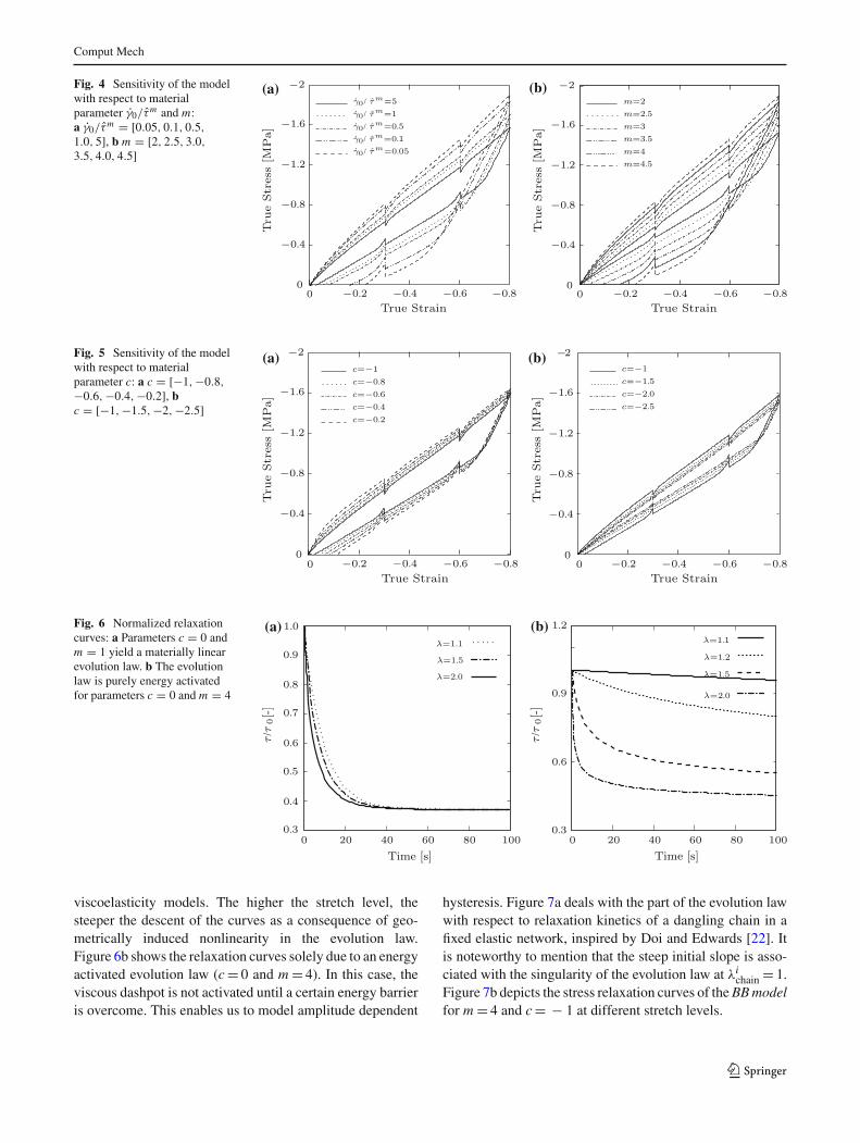
m , the more significantis the hysteresis. On the other hand, as seen in Fig. 4b, thegreater the value of m, the greater is the hysteresis. In Fig. 5aand Fig. 5b, the effect of the parameter c in the range ofc ∈ [−1, 0] and c ≤ −1 is studied, respectively. As thevalue of |c| increases, the amount of hysteresis decreases.However, the slope is steeper at the beginning of the loadingprocess, then the curve attains a certain offset.

4.2 Example 2

In the second example, we carry out a parametric investiga-tion of the evolution law. The material parameters are taken asκ = 1,000 MPa, µ= 0.6 MPa, µv = 0.96 MPa, N = Nv = 8and γ0/τ

m = 0.07 s−1MPa−m. Taking the parameter c= 0and m= 1, the model recovers the isochoric part of the evolu-tion law proposed by Reese and Govindjee [2]. In Fig. 6a, nor-malized relaxation curves for stretch levels λ= 1.1, λ= 1.5and λ= 2.0 are plotted against time. For λ= 1.1, the devi-ation is small from thermodynamical equilibrium and therelaxation curve approaches to the so-called finite linear

123

Comput Mech

Fig. 4 Sensitivity of the modelwith respect to materialparameter γ0/τ

m and m:a γ0/τ

m = [0.05, 0.1, 0.5,

1.0, 5], b m = [2, 2.5, 3.0,

3.5, 4.0, 4.5]

(a) (b)

Fig. 5 Sensitivity of the modelwith respect to materialparameter c: a c = [−1,−0.8,

−0.6,−0.4,−0.2], bc = [−1,−1.5,−2,−2.5]

(a) (b)

Fig. 6 Normalized relaxationcurves: a Parameters c = 0 andm = 1 yield a materially linearevolution law. b The evolutionlaw is purely energy activatedfor parameters c = 0 and m = 4

(a) (b)

viscoelasticity models. The higher the stretch level, thesteeper the descent of the curves as a consequence of geo-metrically induced nonlinearity in the evolution law.Figure 6b shows the relaxation curves solely due to an energyactivated evolution law (c= 0 and m= 4). In this case, theviscous dashpot is not activated until a certain energy barrieris overcome. This enables us to model amplitude dependent

hysteresis. Figure 7a deals with the part of the evolution lawwith respect to relaxation kinetics of a dangling chain in afixed elastic network, inspired by Doi and Edwards [22]. Itis noteworthy to mention that the steep initial slope is asso-ciated with the singularity of the evolution law at λi

chain= 1.Figure 7b depicts the stress relaxation curves of the BB modelfor m= 4 and c= − 1 at different stretch levels.

123

Comput Mech

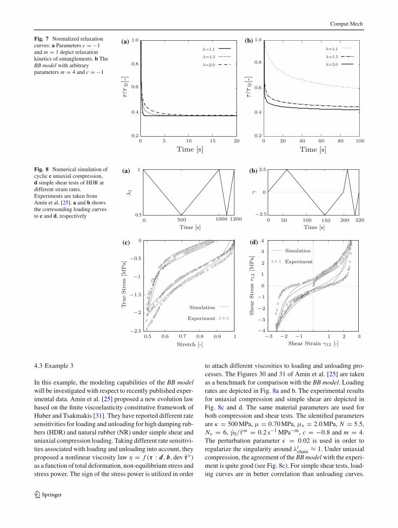
Fig. 7 Normalized relaxationcurves: a Parameters c = −1and m = 1 depict relaxationkinetics of entanglements. b TheBB model with arbitraryparameters m = 4 and c = −1

(a) (b)

Fig. 8 Numerical simulation ofcyclic c uniaxial compression,d simple shear tests of HDR atdifferent strain rates.Experiments are taken fromAmin et al. [25]. a and b showsthe corresonding loading curvesto c and d, respectively

(a) (b)

(c) (d)

4.3 Example 3

In this example, the modeling capabilities of the BB modelwill be investigated with respect to recently published exper-imental data. Amin et al. [25] proposed a new evolution lawbased on the finite viscoelasticity constitutive framework ofHuber and Tsakmakis [31]. They have reported different ratesensitivities for loading and unloading for high damping rub-bers (HDR) and natural rubber (NR) under simple shear anduniaxial compression loading. Taking different rate sensitivi-ties associated with loading and unloading into account, theyproposed a nonlinear viscosity law η = f (τ : d, b, dev τ v)

as a function of total deformation, non-equilibrium stress andstress power. The sign of the stress power is utilized in order

to attach different viscosities to loading and unloading pro-cesses. The Figures 30 and 31 of Amin et al. [25] are takenas a benchmark for comparison with the BB model. Loadingrates are depicted in Fig. 8a and b. The experimental resultsfor uniaxial compression and simple shear are depicted inFig. 8c and d. The same material parameters are used forboth compression and shear tests. The identified parametersare κ = 500 MPa, µ = 0.70 MPa, µv = 2.0 MPa, N = 5.5,Nv = 6, γ0/τ

m = 0.2 s−1 MPa−m, c = −0.8 and m = 4.The perturbation parameter ε = 0.02 is used in order toregularize the singularity around λi

chain ≈ 1. Under uniaxialcompression, the agreement of the BB model with the experi-ment is quite good (see Fig. 8c). For simple shear tests, load-ing curves are in better correlation than unloading curves.

123

Comput Mech

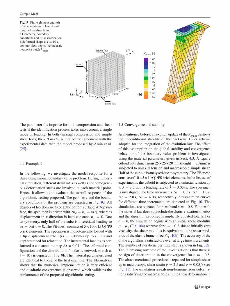
Fig. 9 Finite element analysisof a cube driven in lateral andlongitudinal directions:a Geometry, boundaryconditions and FE discretization,b deformed shape at t = 10 s,contour plots depict the inelasticnetwork stretch λi

chain

(a)

1.00

1.05

1.10

1.15

1.20

1.25

1.30

1.35

1.40

1.45

1.50(b)

The parameter fits improve for both compression and sheartests if the identification process takes into account a singlemode of loading. In both uniaxial compression and simpleshear tests, the BB model is in a better agreement with theexperimental data than the model proposed by Amin et al.[25].

4.4 Example 4

In the following, we investigate the model response for athree-dimensional boundary value problem. During numeri-cal simulation, different strain rates as well as nonhomogene-ous deformation states are involved at each material point.Hence, it allows us to evaluate the overall response of thealgorithmic setting proposed. The geometry and the bound-ary conditions of the problem are depicted in Fig. 9a. Alldegrees of freedom are fixed at the bottom surface. At top sur-face, the specimen is driven with 2u2 = u3 = u(t), whereasdisplacement in x-direction is held constant, u1 = 0. Dueto symmetry, only half of the cube is discretized leading tou1 = 0 at x = 0. The FE-mesh consists of 5×10×15 Q1/P0brick elements. The specimen is monotonically loaded witha tip displacement rate u(t) = 10 mm/s up to t = 1 s andkept stretched for relaxation. The incremental loading is per-formed at constant time step �t = 0.04 s. The deformed con-figuration and the distribution of inelastic network stretch att = 10 s is depicted in Fig. 9b. The material parameters usedare identical to those of the first example. The FE-analysisshows that the numerical implementation is very efficientand quadratic convergence is observed which validates theperformance of the proposed algorithmic setting.

4.5 Convergence and stability

As mentioned before, an explicit update of the λichain destroys

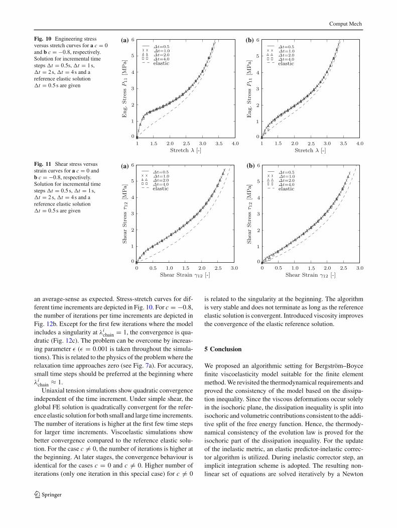
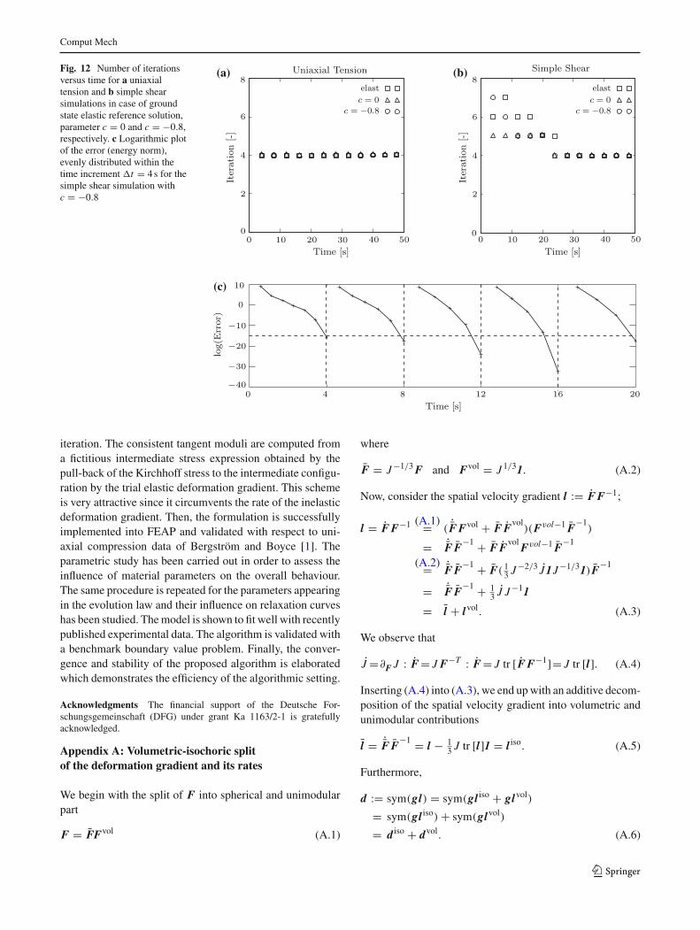
the unconditional stability of the backward Euler schemeadopted for the integration of the evolution law. The effectof this assumption on the global stability and convergencebehaviour of the boundary value problem is investigatedusing the material parameters given in Sect. 4.3. A squarecuboid with dimensions 25×25×20 mm (height= 20 mm) issubjected to uniaxial tension and macroscopic simple shear.Half of the cuboid is analysed due to symmetry. The FE-meshconsists of 10×5×10 Q1/P0 brick elements. In the first set ofexperiments, the cuboid is subjected to a uniaxial tension upto λ = 3.5 with a loading rate of λ = 0.05/s. The specimenis investigated for time increments �t = 0.5 s, �t = 1.0 s,�t = 2.0 s, �t = 4.0 s, respectively. Stress-stretch curvesfor different time increments are depicted in Fig. 10. Thesimulations are repeated for c = 0 and c = −0.8. For c = 0,the material law does not include the chain relaxation kineticsand the algorithm proposed is implicitly updated totally. Forc = 0, the simulation begins with an initial shear modulusµ+µv (Fig. 10a) whereas for c = −0.8, due to initially zeroviscosity, the shear modulus is equivalent to the shear mod-ulus of the elastic branch (see Fig. 10b). The accuracy of theof the algorithm is satisfactory even at large time increments.The number of iterations per time step is shown in Fig. 12a.The interesting outcome of the investigation is that there isno sign of deterioration in the convergence for c = −0.8.The above mentioned procedure is repeated for simple shearup to macroscopic shear strain γ = 2.5 and γ = 0.05/s (seeFig. 11). The simulation reveals non-homogeneous deforma-tions satisfying the macroscopic simple shear deformation in

123

Comput Mech

Fig. 10 Engineering stressversus stretch curves for a c = 0and b c = −0.8, respectively.Solution for incremental timesteps �t = 0.5s, �t = 1 s,�t = 2 s, �t = 4 s and areference elastic solution�t = 0.5 s are given

(a) (b)

Fig. 11 Shear stress versusstrain curves for a c = 0 andb c = −0.8, respectively.Solution for incremental timesteps �t = 0.5 s, �t = 1 s,�t = 2 s, �t = 4 s and areference elastic solution�t = 0.5 s are given

(a) (b)

an average-sense as expected. Stress-stretch curves for dif-ferent time increments are depicted in Fig. 10. For c = −0.8,the number of iterations per time increments are depicted inFig. 12b. Except for the first few iterations where the modelincludes a singularity at λi

chain = 1, the convergence is qua-dratic (Fig. 12c). The problem can be overcome by increas-ing parameter ε (ε = 0.001 is taken throughout the simula-tions). This is related to the physics of the problem where therelaxation time approaches zero (see Fig. 7a). For accuracy,small time steps should be preferred at the beginning whereλi

chain ≈ 1.Uniaxial tension simulations show quadratic convergence

independent of the time increment. Under simple shear, theglobal FE solution is quadratically convergent for the refer-ence elastic solution for both small and large time increments.The number of iterations is higher at the first few time stepsfor larger time increments. Viscoelastic simulations showbetter convergence compared to the reference elastic solu-tion. For the case c �= 0, the number of iterations is higher atthe beginning. At later stages, the convergence behaviour isidentical for the cases c = 0 and c �= 0. Higher number ofiterations (only one iteration in this special case) for c �= 0

is related to the singularity at the beginning. The algorithmis very stable and does not terminate as long as the referenceelastic solution is convergent. Introduced viscosity improvesthe convergence of the elastic reference solution.

5 Conclusion

We proposed an algorithmic setting for Bergström–Boycefinite viscoelasticity model suitable for the finite elementmethod. We revisited the thermodynamical requirements andproved the consistency of the model based on the dissipa-tion inequality. Since the viscous deformations occur solelyin the isochoric plane, the dissipation inequality is split intoisochoric and volumetric contributions consistent to the addi-tive split of the free energy function. Hence, the thermody-namical consistency of the evolution law is proved for theisochoric part of the dissipation inequality. For the updateof the inelastic metric, an elastic predictor-inelastic correc-tor algorithm is utilized. During inelastic corrector step, animplicit integration scheme is adopted. The resulting non-linear set of equations are solved iteratively by a Newton

123

Comput Mech

Fig. 12 Number of iterationsversus time for a uniaxialtension and b simple shearsimulations in case of groundstate elastic reference solution,parameter c = 0 and c = −0.8,respectively. c Logarithmic plotof the error (energy norm),evenly distributed within thetime increment �t = 4 s for thesimple shear simulation withc = −0.8

(a) (b)

(c)

iteration. The consistent tangent moduli are computed froma fictitious intermediate stress expression obtained by thepull-back of the Kirchhoff stress to the intermediate configu-ration by the trial elastic deformation gradient. This schemeis very attractive since it circumvents the rate of the inelasticdeformation gradient. Then, the formulation is successfullyimplemented into FEAP and validated with respect to uni-axial compression data of Bergström and Boyce [1]. Theparametric study has been carried out in order to assess theinfluence of material parameters on the overall behaviour.The same procedure is repeated for the parameters appearingin the evolution law and their influence on relaxation curveshas been studied. The model is shown to fit well with recentlypublished experimental data. The algorithm is validated witha benchmark boundary value problem. Finally, the conver-gence and stability of the proposed algorithm is elaboratedwhich demonstrates the efficiency of the algorithmic setting.

Acknowledgments The financial support of the Deutsche For-schungsgemeinschaft (DFG) under grant Ka 1163/2-1 is gratefullyacknowledged.

Appendix A: Volumetric-isochoric splitof the deformation gradient and its rates

We begin with the split of F into spherical and unimodularpart

F = FFvol (A.1)

where

F = J−1/3 F and Fvol = J 1/31. (A.2)

Now, consider the spatial velocity gradient l := F F−1;

l = F F−1 (A.1)= ( ˙F Fvol + F Fvol

)(Fvol−1 F−1

)

= ˙F F−1 + F F

volFvol−1 F

−1

(A.2)= ˙F F−1 + F( 1

3 J−2/3 J1J−1/31)F−1

= ˙F F−1 + 1

3 J J−11

= l + lvol. (A.3)

We observe that

J=∂F J : F= J F−T : F= J tr [F F−1]= J tr [l]. (A.4)

Inserting (A.4) into (A.3), we end up with an additive decom-position of the spatial velocity gradient into volumetric andunimodular contributions

l = ˙F F−1 = l − 1

3 J tr [l]1 = l iso. (A.5)

Furthermore,

d := sym(gl) = sym(gl iso + glvol)

= sym(gl iso)+ sym(glvol)

= d iso + dvol. (A.6)

123

Comput Mech

Therefore, we can rewrite the Clausius-Planck inequality inthe form

D = [τ vol + τ iso] : [dvol + d iso] − [U + ˙�] ≥ 0. (A.7)

Examining that τ vol : d iso = 0 and τ iso : dvol = 0, (A.7)takes the following form

D = τ vol : dvol + τ iso : d iso − [U + ˙�] ≥ 0. (A.8)

We obtain a stronger constraint by decoupling the volumet-ric and the isochoric parts in the dissipation inequality (A.8)leading to

Dvol = τ vol : dvol − U ≥ 0 (A.9)

and

Diso = τ iso : d iso − ˙� ≥ 0. (A.10)

Hence, one obtains a discrete representation of the Clausius-Duhem inequality for purely isochoric processes of inelas-ticity.

Appendix B: Derivation of the local tangent for Newtoniteration

In this Appendix, the derivation of local tangentKab is shown.We recall the residual expression

ra := εa + �t√2

γ

τv

dev τa − εtra = 0. (B.1)

The local tangent is defined as

Kab := ∂ra

∂εb

∣∣∣∣ε=εk

(B.2)

and can be derived from (B.1)

Kab = δab + �t√2

dev τa∂(γ /τv)

∂εb+ �t√

2

γ

τv

∂dev τa

∂εb. (B.3)

Taking the derivatives in (B.3), one finally obtains the com-pact definition

Kab = δab + β1 dev τaDb + β2Tab, (B.4)

along with the terms defined below:

β1 = �t

2√

2(m − 1)

γ0

τm(λi

chain)cτm−3

v , (B.5)

β2 = �t√2

γ

τv

, (B.6)

Db =3∑

c=1

dev τcTcb, (B.7)

Tab = Tab − 1

3

3∑c=1

Tcb, (B.8)

Tab := ∂τa

∂εb

= 2

3µv

3− λe21

1− λe2r

λaλbδab + 4

9

µv

Nv

1

(1− λe2r )2 λ2

aλ2b.

(B.9)

References

1. Bergström JS, Boyce MC (1998) Constitutive modeling of thelarge strain time–dependent behavior of elastomers. J Mech PhysSolids 46:931–954

2. Reese S, Govindjee S (1998) A theory of finite viscoelasticity andnumerical aspects. Int J Solids Struct 35:3455–3482

3. Lubliner J (1985) A model of rubber viscoelasticity. Mech ResCommun 12:93–99

4. Simo JC, Miehe C (1992) Associative coupled thermoplasticity atfinite strains: formulation, numerical analysis and implementation.ASME J Appl Mech 98:41–104

5. Simo JC (1992) Algorithms for static and dynamic multiplicativeplasticity that preserve the classical return mapping schemes of theinfinitesimal theory. Comput Methods Appl Mech Eng 99:61–112

6. Weber G, Anand L (1990) Finite deformation constitutive equa-tions and a time integration procedure for isotropic hyperelastic-viscoplastic solids. Comput Methods Appl Mech Eng 79:173–202

7. Cuitino A, Ortiz M (1992) A material-independent method forextending stress update algorithms from small-strain plasticity tofinite plasticity with multiplicative kinematics. Eng Comput 9:437–451

8. Ogden R (1972) Large deformation isotropic elastictiy: on the cor-relation of theory and experiment for incompressible rubberlikesolids. Procee R Soc Lond A 326:565–584

9. Areias P, Matous K (2008) Finite element formulation for model-ing nonlinear viscoelastic elastomers. Comput Methods Appl MechEng 197:4702–4717

10. Marckmann G, Verron E (2006) Comparion of hyperelastic modelsfor rubber-like materials. Rubber Chem Technol 12:835–858

11. Treloar LRG (1944) Stress–strain data for vulcanised rubber undervarious types of deformation. Trans Faraday Soc 40:59–70

12. Kawabata S, Matsuda M, Tei K, Kawai H (1998) Experimentalsurvey of the strain energy density function of isoprene rubber vul-canizate. Macromolecules 14:154–162

13. Kaliske M, Heinrich G (1998) An extended tube–model for rubberelasticity: statistical–mechanical theory and finite element imple-mentation. Rubber Chem Technol 72:602–632

14. Miehe C, Göktepe S, Lulei F (2004) A micro–macro approach torubber–like materials. Part I: The non–affine micro–sphere modelof rubber elasticity. J Mech Phys Solids 52:2617–2660

15. Arruda EM, Boyce MC (1993) A three–dimensional constitutivemodel for the large stretch behavior of rubber elastic materials. JMech Phys Solids 41:389–412

16. Green MS, Tobolsky AV (1946) A new approach to the theory ofrelaxing polymeric media. J Chem Phys 14:80–92

17. Lodge AS (1956) A netowork theory of flow birefringence andstress in concentrated polymer solutions. Trans Faraday Soc52:120–130

18. Phan-Thien N (1978) A nonlinear network viscoelastic model. JRheol 22:259–283

19. Tanaka F, Edwards SF (1992) Viscoelastic properties of physicallycrosslinked networks. I: Non–linear stationary viscoelasticity. JNon-Newtonian Fluid Mech 43:247–271

20. Tanaka F, Edwards SF (1992) Viscoelastic properties of physicallycrosslinked networks. II: Dynamic mechanical moduli. J Non-Newtonian Fluid Mech 43:289–309

123

Comput Mech

21. de Gennes PG (1971) Reptation of a polymer chain in the presenceof fixed obstacles. J Chem Phys 55:572–579

22. Doi M, Edwards SF (1986) The theory of polymer dynamics. Clar-endon Press, Oxford

23. Miehe C, Göktepe S (2005) A micro–macro approach to rubber–like materials. Part II: The micro–sphere model of finite rubberviscoelasticity. J Mech Phys Solids 53:2231–2258

24. Miehe C (1998) A constitutive frame of elastoplasticity at largestrains based on the notion of a plastic metric. Int J Solids Struct35:3859–3897

25. Amin AFMS, Lion A, Sekita S, Okui Y (2006) Nonlinear depen-dence of viscosity in modeling the rate-dependent response ofnatural and high damping rubbers in compression and shear:Experimental identification and numerical verification. Int J Plast22:1610–1657

26. Cohen A (1991) A Padé approximant to the inverse langevin func-tion. Rheol Acta 30:270–273

27. Diani J, Gilormini P (2005) Combining the logarithmic strain andthe full-network model for a better understanding of the hyper-elastic behaviour of rubber-like materials. J Mech Phys Solids53:2579–2596

28. Simo JC, Taylor RL, Pister KS (1985) Variational and projectionmethods for the volume constraint in finite deformation elasto–plasticity. Comput Methods Appl Mech Eng 51:177–208

29. Miehe C (1994) Aspects of the formulation and finite elementimplementation of large strain isotropic elasticity. Int J NumerMethods Eng 37:1981–2004

30. Bergström JS, Boyce MC (2001) Constitutive modeling of thetime-dependent and cyclic loading of elastomers and applicationto soft biological tissues. Mech Mater 33:523–530

31. Huber N, Tsakmakis C (2000) Finite deformation viscoelasticitylaws. Mech Mater 32:1–18

123