1

Benchmarking within a DEA framework: setting the closest targets and identifying

peer groups with the most similar performances

José L. Ruiz and Inmaculada Sirvent

Centro de Investigación Operativa. Universidad Miguel Hernández. Avd. de la Universidad, s/n

03202-Elche (Alicante), SPAIN

June, 2019

Abstract

Data Envelopment Analysis (DEA) is widely used as a benchmarking tool for improving performance

of organizations. For that purpose, DEA analyses provide information on both target setting and peer

identification. However, the identification of peers is actually a by-product of DEA. DEA models seek a

projection point of the unit under evaluation on the efficient frontier of the production possibility set (PPS),

which is used to set targets, while peers are identified simply as the members of the so-called reference sets,

which consist of the efficient units that determine the projection point as a combination of them. In practice,

the selection of peers is crucial for the benchmarking, because organizations need to identify a peer group in

their sector or industry that represent actual performances from which to learn. In this paper, we argue that

DEA benchmarking models should incorporate into their objectives criteria for the selection of suitable

benchmarks among peers, in addition to considering the setting of appropriate targets (as usual). Specifically,

we develop models having two objectives: setting the closest targets and selecting the most similar reference

sets. Thus, we seek to establish targets that require the less effort from organizations for their achievement in

addition to identifying peer groups with the most similar performances, which are potential benchmarks to

emulate and improve.

Keywords: Data Envelopment Analysis; Benchmarking; Peer identification; Target Setting.

1. Introduction

Managers of organizations use benchmarking for the evaluation of performance in comparison

to best practices of others within a peer group of firms in an industry or sector. In the best-practice

benchmarking process, the identification of the best firms makes it possible to set targets, taking into

account considerations related to the similarity of performances or the effort needed for their

achievement, in order for organizations to ultimately learn from them in planning improvements.

Data Envelopment Analysis (DEA) (Charnes et al., 1978) has been widely used as a

benchmarking tool for improving performance of decision making units (DMUs). Some recent papers

dealing with DEA and benchmarking include Adler et al. (2013), which uses network DEA, Zanella

et al. (2013), which uses a model based on a novel specification of weight restrictions, Dai and

Kuosmanen (2014), which combines DEA with clustering methods, Yang et al. (2015), which uses

DEA to create a dynamic benchmarking system, Gouveia et al. (2015), which combines DEA and

2

multi criteria decision analysis (MCDA), Daraio and Simar (2016), which deals with benchmarking

and directional distances, Gomes Júnior et al. (2016), which uses non-radial efficiencies in a

benchmarking analysis based on alternative targets, and Ghahraman and Prior (2016) and Lozano and

Calzada-Infante (2018), which propose stepwise benchmarking approaches.

In DEA, the performance of DMUs is evaluated through setting targets on the frontier of the

production possibility set (PPS) formed by the efficient units, which can be seen as a best practice

frontier in the circumstance of benchmarking (see Cook et al. (2014) for discussions). Specifically,

targets are the coordinates of a projection point of the unit under evaluation on to the efficient frontier,

which result from a combination of efficient DMUs on a face of such frontier. Those efficient DMUs

are typically grouped in the so-called “reference sets”. Thus, as stated in Thanassoulis et al. (2008),

target settings and peer identification are largely the purpose of the DEA analysis (beside the

efficiency score). In particular, where the DMU is Pareto-inefficient: identifying efficient DMUs

whose operating practices it may attempt to emulate to improve its performance, and estimating

target input-output levels that the DMU should in principle be capable of attaining under efficient

operation is an important part of the information most readily obtainable from a DEA analysis (see

also Thanassoulis (2001)).

The selection of actual referents is particularly crucial in the benchmarking, because

organizations need to identify a peer group in their sector or industry that represent actual

performances from which to learn. We note that projections in DEA represent virtual DMUs that

result from actual units by assuming some postulates, while efficient DMUs in the reference sets are

actual DMUs (peers). As said before, DEA analyses provide information on both target setting and

peer identification. However, DEA models are primarily concerned with target setting (e.g., the

closest targets), while the identification of the peers (for purposes of benchmarking) can actually be

seen as a by-product. That is, DEA models implement objectives that deal with the projection point

that determines the targets, while the selection of the efficient DMUs that constitute the reference set

is made without following any specific criterion for the benchmarking. In practice, the efficient

DMUs in the reference sets are used for the benchmarking, for example by means of radar charts that

allow us to compare the units under assessment against both targets and peers in order to evaluate

performance and plan for improvements (see Thanassoulis et al., 2008). But it is obvious that a

selection of peers based only on grounds of belonging to a DEA reference set, which simply means

participating in the combination of efficient DMUs that lead to the projection point, does not

necessarily ensure an appropriate selection of benchmarks, unless they are chosen following some

additional desirable criterion for the benchmarking.

3

In this paper, we pay special attention to this aspect of the DEA analysis, namely the

identification of peers for purposes of benchmarking. In the proposed approach, peer groups are

identified as DEA reference sets associated with a given projection point (as usual), but they are

selected following some additional desirable criteria for the benchmarking. Bearing in mind the

discussion above, it can be argued that DEA benchmarking models should incorporate into the

formulations objectives related to the selection of suitable benchmarks among peers, in addition to

considering the setting of appropriate targets. Specifically, we seek an approach based on models that

implement criteria of closeness between actual inputs and/or outputs and targets, on one hand, and

similarity of performances between actual DMUs and peers, on the other.

This approach is developed within the context of non-radial DEA models. As stated in

Thanassoulis et al. (2008), non-radial models are the appropriate instruments for target setting and

benchmarking, because they ensure that the identified targets lie on the Pareto-efficient subset of the

frontier. In particular, the models formulated here are in line with those that minimize the distance to

the efficient frontier and set the closest targets. Closest targets minimize the gap between actual

performances and best practices, thus showing DMUs the way for improvement with as little effort

as possible. These models have made an important contribution to DEA as tool for the best-practice

benchmarking of DMUs. In fact, there is already a large and growing body of research on setting

closest targets and benchmarking. Portela et al. (2003) deals with similarity in DEA as closeness

between actual inputs and outputs of units under evaluation and targets, and propose determining

projection points as similar as possible to those units. Aparicio et al. (2007) solve theoretically the

problem of minimizing the distance to the efficient frontier by using a mixed integer linear problem

(MILP) that is used to set the closest targets. For the same purposes of target setting and

benchmarking, the ideas in the latter paper are extended in Ramón et al. (2016) to models with weight

restrictions, in Ruiz and Sirvent (2016) for developing a common benchmarking framework, in

Aparicio et al. (2017) to oriented models, in Cook et al. (2017) for the benchmarking of DMUs

classified in groups, in Ramón et al. (2018), which propose a sequential approach for the

benchmarking, in Ruiz and Sirvent (2018) to models that incorporate information on goals, and in

Cook et al. (2019) for a benchmarking approach within the context of pay-for-performance incentive

plans1. In the present paper, the models developed have two objectives: minimizing the gap between

actual inputs and/or outputs and targets and minimizing the dissimilarities between actual

performances and those of the members of the reference sets. Thus, these models will allow us to

1 We note that the idea of closeness to the efficient frontier has also been investigated for purposes of developing efficiency

measures that satisfy some desirable properties. See Ando (2017), Aparicio and Pastor (2014), Fukuyama et al. (2014a,

2014b) and Fukuyama et al. (2016).

4

evaluate performance in terms of targets that require the less effort for their achievement while at the

same time identifying peers with the most similar performances to emulate and improve.

We develop non-oriented and oriented DEA benchmarking models, taking into account in

addition the specification of returns to scale (variable or constant). The two objectives are

implemented in most cases through the closeness between vectors of inputs and/or outputs, except

for the selection of the reference set in the constant returns to scale (CRS) case, wherein the similarity

of performances between actual DMUs and peers is assessed in terms of the deviations between the

corresponding mixes of inputs and outputs. In all of the models, a parameter is included in the

formulations that allows us to adjust the importance attached to each of the two objectives. Through

the specification of such parameter, a series of targets and reference sets can be generated. These

series provide managers with more flexibility in target setting and benchmark selection, both for

evaluating performance and for future planning. This is illustrated through an example in which

teaching performance of public Spanish universities is evaluated.

The paper is organized as follows: In section 2, we develop a bi-objective DEA non-oriented

benchmarking model that allows to setting the closest targets and selecting the closest reference set.

Section 3 addresses the case of oriented models (either to inputs or to outputs). Section 4 addresses

the case of having a technology in which constant returns to scale is assumed. In section 5 we examine

an example for purposes of illustration. Last section concludes.

2. A model for setting the closest targets and selecting the closest reference set

Throughout this section, we consider that we have n DMUs whose performances are to be

evaluated in terms of m inputs and s outputs. These are denoted by j jX ,Y , j 1,...,n, where

j 1j mj mX x ,..., x 0 ,

j 1,...,n, and j 1j sj sY y ,..., y 0 ,

j 1,...,n. For the benchmarking, we

assume a variable returns to scale (VRS) technology (Banker et al., 1984). Thus, the production

possibility set (PPS), T (X,Y) X can produce Y , can be characterized as

n n n

j j j j j j

j 1 j 1 j 1

T X,Y X X , Y Y , 1, 0

.

For a given DMU0, the DEA models that set the closest targets find a projection point 0 0ˆ ˆX ,Y

by minimizing the distance from that unit to the points on the efficient frontier of T, (T), dominating

0 0X ,Y . The problem below provides a general formulation of such models

5

0 0 0 0

0 0

0 0 0 0

ˆ ˆMin d X ,Y , X ,Y

s.t. :

ˆ ˆX ,Y (T)

ˆ ˆX ,Y dominates X ,Y

(1)

Typically, the distance between two points of T is calculated by using the following weighted

L1-norm: m s

i0 i0 r0 r0

0 0 0 0 0 0 0 01

i 1 r 1i0 r0

ˆ ˆx x y yˆ ˆ ˆ ˆd X ,Y , X ,Y X ,Y X ,Yx y

(note that

we do not use absolute values because the projection point dominates DMU0). If deviations between

actual inputs and outputs and the coordinates of the projection are expressed by using the classical

slacks, then the model below provides an operational formulation of (1) (see Aparicio et al., 2007)

m si0 r0

i 1 r 1i0 r0

j ij i0 i0

j E

j rj r0 r0

j E

j

j E

m s

i ij r rj 0 j

i 1 r 1

i

r

j j

j j

i0 r0

0

s sMin

x y

s.t. :

x x s i 1,...,m

y y s r 1,...,s

1

v x u y u 0 j E

v 1 i 1,...,m

u 1 r 1,...,s

0 j E

, 0 j E

s , s 0 i, r

u free

(2)

where E is the set of extreme efficient DMUs in T.

Remark. In Aparicio et al. (2007) the constraints j j 0, j E, are equivalently expressed by using

the classical big M and binary variables. Eventually, in practice, we use Special Ordered Sets (SOS)

(Beale and Tomlin, 1970) for solving the resulting problem. SOS Type 1 is a set of variables where

6

at most one variable may be nonzero. Therefore, if we remove these constraints from the formulation

and define instead a SOS Type 1 for each pair of variables j j, , j E, then it is ensured that j

and j cannot be simultaneously positive for DMUj’s, j E. As a result, the DMUj’s in the reference

set of DMU0 belong all to the same supporting hyperplane of the T at the projection point of that unit.

SOS variables have already used for solving models like (2) in Ruiz and Sirvent (2016, 2018),

Aparicio et al. (2017), Cook et al. (2017) and Cook et al. (2019).

Model (2) finds the closest dominating projection point to DMU0 on the efficient frontier of

T. The coordinates of such point allow us to set targets in terms of which the performance of DMU0

can be evaluated. Specifically, these targets can be expressed by using the optimal solutions of (2) as

i0 i0 i0 j ij

j E

r0 r0 r0 j rj

j E

x x s x , i 1,...,m

y y s y , r 1,...,s

(3)

Model (2) allows us also to identify a reference set for DMU0, 0 j jRS DMU 0 (as

usual in DEA analyses). As said in the introduction, the DMUs in 0RS (actual units) are typically

used for benchmarking purposes. Note, however, that 0RS is identified by model (2) as a by-product

of setting the closest targets to DMU0, because no specific desirable criterion for the benchmarking

is followed in its selection. 0RS simply consists of the efficient DMUs on a face of (T) that

determine the projection of DMU0, 0 0ˆ ˆX ,Y , as a combination of them. As a result, in practice it

often happens that peers with quite dissimilar performances to that of DMU0 are selected as

benchmarks for its evaluation, simply because they are members of the combination of efficient

DMUs that determines the closest targets.

For these reasons, in this paper we argue that DEA benchmarking models should consider in

their objectives not only the setting of appropriate targets but also the selection of suitable benchmarks

among peers. Specifically, the models we develop here consider the following two objectives:

Objective 1: The targets set should be as close as possible to the actual inputs and outputs of the unit

under evaluation.

7

Objective 2: The selected reference sets should consist of peers representing actual performances as

similar as possible to that of the unit under evaluation.

Objective 1 seeks to set targets that require the least possible effort from the DMU0 for their

achievement. Objective 2 seeks to identify a peer group representing potential benchmarks that DMU0

can emulate as easily as possible for improving performance. Model (1) only considers the first

objective in its formulation. To address the second objective, 0RS can be selected by minimizing the

distance from DMU0 to all of its members. In order to do so, we follow here a minmax approach, that

is, we minimize the distance from DMU0 to the unit in the reference set with most dissimilar

performance. Actually, using a minmax approach for minimizing globally the distances from DMU0

to all the members of RS0 is equivalent to minimizing the Hausdorff distance from a point to a finite

set (in a metric space). In this context, the Hausdorff distance, which we denote by

H 0 0 0d X ,Y ,RS , is defined as

0 0 0

H 0 0 0

m si0 ij r0 rj

0 0 j j 0 0 j j1j RS j RS j RS

i 1 r 1i0 r0

d X ,Y ,RS

x x y ymax d X ,Y , X ,Y max X ,Y X ,Y max

x y

(4)

Ideally, one would like to minimize simultaneously both distances 0 0 0 0ˆ ˆd X ,Y , X ,Y and

H 0 0 0d X ,Y ,RS for target setting and peer identification. However, it is obvious that the targets

that minimize 0 0 0 0ˆ ˆd X ,Y , X ,Y will not be necessarily the coordinates of a projection point

determined by the closest peers to DMU0 (that is, those that minimize H 0 0 0d X ,Y ,RS ), and the

other way around too. As a compromise between these two objectives, we propose to minimize a

convex combination of them

0 0 0 0 H 0 0 0ˆ ˆd X ,Y , X ,Y 1 d X ,Y ,RS , (5)

8

where 0 1. This will provide us with non-dominated solutions2. Through the specification of

, we may adjust the importance that is attached to each of the two objectives. The specification

1 leads to the closest targets to DMU0 on (T), that is, those provided by model (2). However,

as said before, the selection of suitable benchmarks among peers in that case is not considered as an

objective in the model. As decreases, the selection of closer peers is considered together with the

setting of closer targets. Obviously, selecting peers with more similar performance could entail setting

targets that are more demanding, although that is not always necessarily the case in real applications,

as will be shown later in the empirical illustration. In practice, it may be useful to provide a series of

targets and peer groups that are generated by specifying values for in a grid between 0 and 1 (this

approach has already been used in Stewart (2010) for benchmarking models that incorporate

management goals). These series may offer different views on organizations’ performance and

provide managers with different alternatives that they can consider both in evaluating performance

and in planning improvements. This all will be illustrated in section 5.

Bearing in mind the above, a model that sets the closest targets that are sought for DMU0

while at the same time selecting the closest reference set associated with such targets (for a given )

can be formulated as follows

0 0 0 0 H 0 0 0

0 0

0 0 0 0

ˆ ˆMin d X ,Y , X ,Y 1 d X ,Y ,RS

s.t. :

ˆ ˆX ,Y (T)

ˆ ˆX ,Y dominates X ,Y

(6)

In terms of the classical slacks, the following model provides an operational formulation of

(6)

2 To ensure non-dominated solutions in the cases α=0 and 1, a second stage would have to be carried out, in which the

objective that is not considered in (5) is minimized subject to (5) equals the optimal value obtained in the first stage.

9

m si0 r0

0

i 1 r 1i0 r0

j ij i0 i0

j E

j rj r0 r0

j E

j

j E

m s

i ij r rj 0 j

i 1 r 1

i

r

j j

j j

0 0 j j j

s sMin (1 )z

x y

s.t. :

x x s i 1,...,m

y y s r 1,...,s

1

v x u y u 0 j E

v 1 i 1,...,m

u 1 r 1,...,s

0 j E

I j E

d X ,Y , X , Y I

0

j

j j

i0 r0

0

0

z j E

I 0,1 j E

, 0 j E

s , s 0 i, r

z 0

u free

(7)

where the scalars m s

i0 ij r0 rj

0 0 j j

i 1 r 1i0 r0

x x y yd X ,Y , X ,Y ,

x y

j E, are to be calculated prior

to solving the model.

Model (7) minimizes both 0 0 0 0ˆ ˆd X ,Y , X ,Y and H 0 0 0d X ,Y ,RS by using a minsum

approach through the parameter . Like in (2), the set of constraints of model (7) restricts the search

of projections to points on (T) that dominate DMU0. Note that because of the constraints j j 0 ,

j E , if j 0 then j 0 , j E . This means that if DMUj in E belongs to a reference set of DMU0

then it is necessarily on the hyperplane 0v X u Y u 0. Thus, all the DMUs in a reference set

are on a same face of (T) , because they all are on the same supporting hyperplane of T, whose

coefficients are non-zero. Therefore, solving (7) leads to a projection point of DMU0, 0 0ˆ ˆX ,Y , onto

a face of (T) spanned by the DMUs in the reference set, 0 j jRS DMU 0 . However, in (7),

0RS is identified by minimizing in addition the distance from DMU0 to that set (in terms of the

10

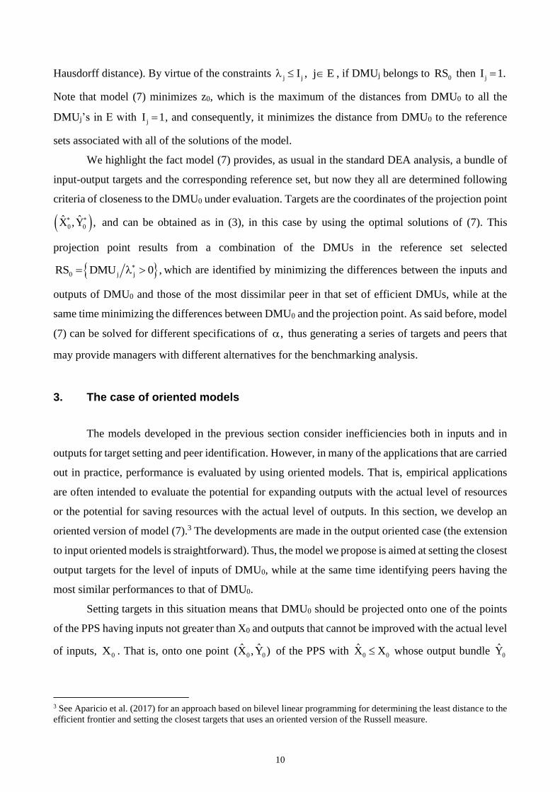
Hausdorff distance). By virtue of the constraints j jI , j E , if DMUj belongs to 0RS then jI 1.

Note that model (7) minimizes z0, which is the maximum of the distances from DMU0 to all the

DMUj’s in E with jI 1 , and consequently, it minimizes the distance from DMU0 to the reference

sets associated with all of the solutions of the model.

We highlight the fact model (7) provides, as usual in the standard DEA analysis, a bundle of

input-output targets and the corresponding reference set, but now they all are determined following

criteria of closeness to the DMU0 under evaluation. Targets are the coordinates of the projection point

0 0ˆ ˆX ,Y , and can be obtained as in (3), in this case by using the optimal solutions of (7). This

projection point results from a combination of the DMUs in the reference set selected

0 j jRS DMU 0 , which are identified by minimizing the differences between the inputs and

outputs of DMU0 and those of the most dissimilar peer in that set of efficient DMUs, while at the

same time minimizing the differences between DMU0 and the projection point. As said before, model

(7) can be solved for different specifications of , thus generating a series of targets and peers that

may provide managers with different alternatives for the benchmarking analysis.

3. The case of oriented models

The models developed in the previous section consider inefficiencies both in inputs and in

outputs for target setting and peer identification. However, in many of the applications that are carried

out in practice, performance is evaluated by using oriented models. That is, empirical applications

are often intended to evaluate the potential for expanding outputs with the actual level of resources

or the potential for saving resources with the actual level of outputs. In this section, we develop an

oriented version of model (7).3 The developments are made in the output oriented case (the extension

to input oriented models is straightforward). Thus, the model we propose is aimed at setting the closest

output targets for the level of inputs of DMU0, while at the same time identifying peers having the

most similar performances to that of DMU0.

Setting targets in this situation means that DMU0 should be projected onto one of the points

of the PPS having inputs not greater than X0 and outputs that cannot be improved with the actual level

of inputs, 0X . That is, onto one point 0 0ˆ ˆ(X ,Y ) of the PPS with 0 0X X whose output bundle 0Y

3 See Aparicio et al. (2017) for an approach based on bilevel linear programming for determining the least distance to the

efficient frontier and setting the closest targets that uses an oriented version of the Russell measure.

11

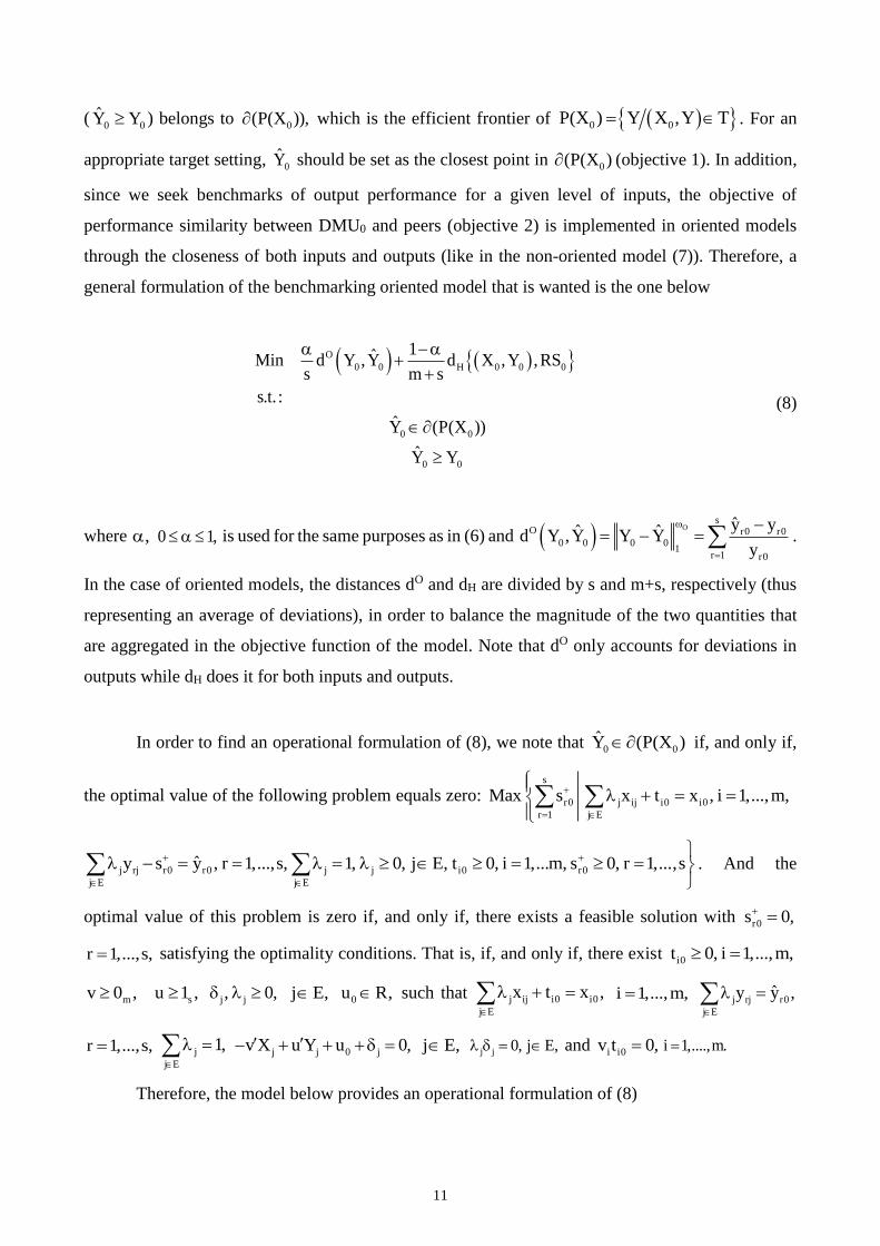
( 0 0Y Y ) belongs to 0(P(X )), which is the efficient frontier of 0 0P(X ) Y X ,Y T . For an

appropriate target setting, 0Y should be set as the closest point in 0(P(X ) (objective 1). In addition,

since we seek benchmarks of output performance for a given level of inputs, the objective of

performance similarity between DMU0 and peers (objective 2) is implemented in oriented models

through the closeness of both inputs and outputs (like in the non-oriented model (7)). Therefore, a

general formulation of the benchmarking oriented model that is wanted is the one below

O

0 0 H 0 0 0

0 0

0 0

1ˆMin d Y ,Y d X ,Y ,RSs m s

s.t. :

Y (P(X ))

Y Y

(8)

where , 0 1, is used for the same purposes as in (6) and O

sO r0 r0

0 0 0 01

r 1 r0

y yˆ ˆd Y ,Y Y Yy

.

In the case of oriented models, the distances dO and dH are divided by s and m+s, respectively (thus

representing an average of deviations), in order to balance the magnitude of the two quantities that

are aggregated in the objective function of the model. Note that dO only accounts for deviations in

outputs while dH does it for both inputs and outputs.

In order to find an operational formulation of (8), we note that 0 0Y (P(X ) if, and only if,

the optimal value of the following problem equals zero: s

r0 j ij i0 i0

r 1 j E

Max s x t x , i 1,...,m,

j rj r0 r0 j j i0 r0

j E j E

ˆy s y , r 1,...,s, 1, 0, j E, t 0, i 1,...m, s 0, r 1,...,s

. And the

optimal value of this problem is zero if, and only if, there exists a feasible solution with r0s 0,

r 1,...,s, satisfying the optimality conditions. That is, if, and only if, there exist i0t 0, i 1,...,m,

mv 0 , su 1 , j j, 0, j E, 0u R, such that j ij i0 i0

j E

x t x ,

i 1,...,m, j rj r0

j E

ˆy y ,

r 1,...,s, j

j E

1,

j j 0 jv X u Y u 0, j E, j j 0, j E, and i i0v t 0, i 1,....,m.

Therefore, the model below provides an operational formulation of (8)

12

sr0

0

r 1 r0

j ij i0 i0

j E

j rj r0 r0

j E

j

j E

m s

i ij r rj 0 j

i 1 r 1

r

j j

i i0

j j

0 0 j j j 0

j

s 1Min z

s y m s

s.t. :

x x t i 1,...,m

y y s r 1,...,s

1

v x u y u 0 j E

u 1 r 1,...,s

0 j E

v t 0 i 1,...,m

I j E

d X ,Y , X ,Y I z j E

I 0,1 j E

j j

r0

i i0

0

0

, 0 j E

s 0 r 1,...,s

v , t 0 i 1,...,m

z 0

u free

(9)

Targets for the outputs in terms of the optimal solutions of model (9) can be obtained as

r0 r0 r0 j rj

j E

y y s y , r 1,...,s

, the reference set for DMU0 being 0 j jRS DMU 0 , as

usual.

4. The constant returns to scale (CRS) case

The specification of returns to scale for the technology has some implications when the

objective of performance similarity for peer identification (objective 2) is addressed in the

formulation of DEA benchmarking models. In the VRS case, the two objectives established in this

paper for the benchmarking models can be implemented through the closeness between the inputs

and/or outputs of DMU0 and both targets and the inputs and/or outputs of the peers in the reference

set. However, if constant returns to scale (CRS) is assumed, the similarity of performances between

DMU0 and the actual efficient DMUs in the reference set cannot be measured in terms of closeness

13

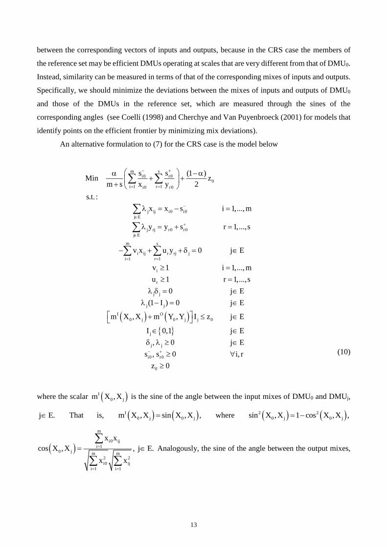
between the corresponding vectors of inputs and outputs, because in the CRS case the members of

the reference set may be efficient DMUs operating at scales that are very different from that of DMU0.

Instead, similarity can be measured in terms of that of the corresponding mixes of inputs and outputs.

Specifically, we should minimize the deviations between the mixes of inputs and outputs of DMU0

and those of the DMUs in the reference set, which are measured through the sines of the

corresponding angles (see Coelli (1998) and Cherchye and Van Puyenbroeck (2001) for models that

identify points on the efficient frontier by minimizing mix deviations).

An alternative formulation to (7) for the CRS case is the model below

m si0 r0

0

i 1 r 1i0 r0

j ij i0 i0

j E

j rj r0 r0

j E

m s

i ij r rj j

i 1 r 1

i

r

j j

j j

I O

0 j 0 j

s s (1 )Min z

m s x y 2

s.t. :

x x s i 1,...,m

y y s r 1,...,s

v x u y 0 j E

v 1 i 1,..., m

u 1 r 1,...,s

0 j E

(1 I ) 0 j E

m X ,X m Y ,Y

j 0

j

j j

i0 r0

0

I z j E

I 0,1 j E

, 0 j E

s , s 0 i, r

z 0

(10)

where the scalar I

0 jm X ,X is the sine of the angle between the input mixes of DMU0 and DMUj,

j E. That is, I

0 j 0 jm X ,X sin X ,X , where 2 2

0 j 0 jsin X ,X 1 cos X ,X ,

m

i0 ij

i 10 j

m m2 2

i0 ij

i 1 i 1

x x

cos X ,X ,

x x

j E. Analogously, the sine of the angle between the output mixes,

14

O

0 jm Y ,Y , j E, can be defined. Note that these scalars have to be calculated prior to solving the

model.

Model (10) works in a similar manner as (7). The main difference is in that objective 2 is now

expressed in terms of similarities of input and output mixes between DMU0 and the DMUj’s in a

reference set. In (7) we use the L1-distance (weighted), which aggregates the deviations between

vectors of inputs and outputs, while in (10) we also aggregate the deviations between the mixes of

inputs and outputs as measured through the sines of the corresponding angles. Again, the two

components of the objective function are divided by a constant in order to balance their magnitude.

Specifically, the one associated with objective 1 is divided by m+s while that of objective 2 is divided

by 2. The constraints j j(1 I ) 0 ensure that, if j 0, then jI 1 (these non-linear constraints can

be handled by using SOS variables as explained in the Remark on model (2)). Therefore, model (10)

seeks to minimize the maximum deviation between the mixes of inputs and outputs of DMU0 and

those of the DMUj’s in the corresponding reference set. Finally, note that the convexity constraint

and the variable u0 have been removed as the result of assuming a CRS technology.

5. Illustrative example

For purposes of illustration only, in this section we apply the proposed approach to the

evaluation of teaching performance of public Spanish universities. The existing regulatory framework

in Spain emphasizes the importance of undergraduate education as a key issue in the performance of

the universities, in line with the higher education policies and practices in Europe. This regulation

also raises the need to design mechanisms for the evaluation of the universities’ teaching

performance, independently from their performance in other areas, such as those of research or

knowledge transfer. Specifically, after the reforms that were motivated by the convergence with

European Space of Higher Education (ESHE), the new degrees are required to have a quality

assurance system available, which must include procedures for the evaluation and improvement of

the quality of teaching and of the academic staff.

We carry out an evaluation of teaching performance from a perspective of benchmarking and

target setting. The practice of benchmarking is growing among universities, which see comparisons

with their peers as an opportunity to analyze their own strengths and weaknesses and to establish

directions for improving performance. In this study, we pay special attention to the selection of

suitable benchmarks among universities through the approach that has been proposed here, which

allows us in addition to set the closest targets to the universities under evaluation.

15

The public Spanish universities may be seen as a set of homogeneous DMUs that undertake

similar activities and produce comparable results regarding teaching performance, so that a common

set of outputs can be defined for their analysis. Specifically, for the selection of the outputs, we only

take into consideration variables that represent aspects of performance explicitly mentioned as

requirements in the section “Expected Results” of the Royal Order RD 1393/2007, such as graduation,

drop out and progress of students. As for the inputs, we consider academic staff and expenditures, as

two variables that account for human and physical capital, and total enrollments, as a proxy of the

size of the universities, which has a significant impact on the performance of European universities

(see Daraio et al. (2015)). We adopt the academic year 2014-15 as the reference year (this approach

has been followed in similar models used for performance evaluation of universities; see, for example,

Agasisti and Dal Bianco (2009)). The variables considered are defined as explained below:

OUTPUTS

- GRADUATION (GRAD): Total number of students that complete the programme of studies

within the planned time.

- RETENTION (RET): Total number of students enrolled for the first time in the academic year

2012-13 that keep enrolled at the university.

- PROGRESS (PROG): Total number of passed credits4.

INPUTS

- TOTAL ENROLLMENT (ENR): Total number of enrollments.

- ACADEMIC STAFF (ASTF): Full-time equivalent academic staff.

- EXPENDITURE (EXP): This input exactly accounts for expenditure on goods and services after

the item corresponding to works carried out by other (external) companies has been removed.

EXP thus reflects the budgetary effort made by the universities in the delivery of their activities.

Data for these variables have been taken from the corresponding report by the Conference of

Rectors of the Spanish Universities (CRUE). The sample consists of 38 (out of 48) public Spanish

universities. Table 1 reports a descriptive summary.

Table 1. descriptive summary

4 Credit is the unit of measurement of the academic load of the subject of a programme.

16

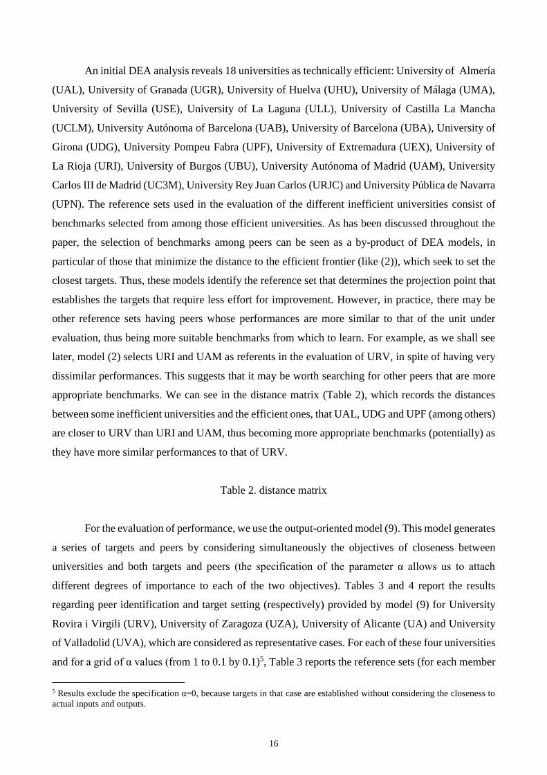
An initial DEA analysis reveals 18 universities as technically efficient: University of Almería

(UAL), University of Granada (UGR), University of Huelva (UHU), University of Málaga (UMA),

University of Sevilla (USE), University of La Laguna (ULL), University of Castilla La Mancha

(UCLM), University Autónoma of Barcelona (UAB), University of Barcelona (UBA), University of

Girona (UDG), University Pompeu Fabra (UPF), University of Extremadura (UEX), University of

La Rioja (URI), University of Burgos (UBU), University Autónoma of Madrid (UAM), University

Carlos III de Madrid (UC3M), University Rey Juan Carlos (URJC) and University Pública de Navarra

(UPN). The reference sets used in the evaluation of the different inefficient universities consist of

benchmarks selected from among those efficient universities. As has been discussed throughout the

paper, the selection of benchmarks among peers can be seen as a by-product of DEA models, in

particular of those that minimize the distance to the efficient frontier (like (2)), which seek to set the

closest targets. Thus, these models identify the reference set that determines the projection point that

establishes the targets that require less effort for improvement. However, in practice, there may be

other reference sets having peers whose performances are more similar to that of the unit under

evaluation, thus being more suitable benchmarks from which to learn. For example, as we shall see

later, model (2) selects URI and UAM as referents in the evaluation of URV, in spite of having very

dissimilar performances. This suggests that it may be worth searching for other peers that are more

appropriate benchmarks. We can see in the distance matrix (Table 2), which records the distances

between some inefficient universities and the efficient ones, that UAL, UDG and UPF (among others)

are closer to URV than URI and UAM, thus becoming more appropriate benchmarks (potentially) as

they have more similar performances to that of URV.

Table 2. distance matrix

For the evaluation of performance, we use the output-oriented model (9). This model generates

a series of targets and peers by considering simultaneously the objectives of closeness between

universities and both targets and peers (the specification of the parameter α allows us to attach

different degrees of importance to each of the two objectives). Tables 3 and 4 report the results

regarding peer identification and target setting (respectively) provided by model (9) for University

Rovira i Virgili (URV), University of Zaragoza (UZA), University of Alicante (UA) and University

of Valladolid (UVA), which are considered as representative cases. For each of these four universities

and for a grid of α values (from 1 to 0.1 by 0.1)5, Table 3 reports the reference sets (for each member

5 Results exclude the specification α=0, because targets in that case are established without considering the closeness to

actual inputs and outputs.

17

of a reference set, its distance to the university under evaluation is recorded between brackets) and

Table 4 reports the targets. The last column of each table records the distance components that are

aggregated in the objective function of (9), that is, those regarding the distances from the university

under evaluation both to its projection on the efficient frontier ( Od 3 ) and to its reference set (Hd 6 ).

The rows α=1 actually record the results provided by model (2), which sets the closest targets on the

efficient frontier. They are therefore included in the tables as the reference specification. As α

decreases, model (9) attaches more importance to the selection of closer benchmarks among peers.

The changes in the distance Od 3 provide us with an insight into the extra effort that is needed for

the achievement of the new targets, while the changes in Hd 6 allow us to assess the degree to which

the new reference sets are more similar.

In the evaluation of URV with model (2) (α=1), the following reference set is found

1

URV UDG,UPF,URR I,UAM . However, when α is lower than 1, model (9) identifies a new

reference set URVR UDG,UPF,UC3M , (α<1). Therefore, solving the model suggests removing

URI and UAM from 1

URVR (because, as said before, they are quite different from URV) and

considering UC3M whose performance is more similar. Note that Hd 6 reduces from 0.976 to 0.346

when the reference set is changed. It is also important to highlight that the output targets associated

with α=1 and those of α’s lower than 1 are quite similar (see in Table 4 that Od 3 only raises from

0.107 to 0.161 when changing the reference set). This means that model (9) allows us to set targets

that require a similar effort as that needed with the closest targets for their achievement, albeit those

targets are associated with a reference set consisting of peers whose performances are more similar

to that of URV, thus being more appropriate benchmarks. The same happens with UZA, because the

reference set provided by (2) includes some universities that are very dissimilar from UZA (UBA and

UPN) while the one provided by (9) suggests other peers that are more like this university (UCLM

and UAB). Now, Hd 6 reduces from 0.728 to 0.212, so, again, there would be no substantial effect

on target setting ( Od 3 only raises from 0.051 to 0.087); perhaps, a little extra effort in GRAD should

be made, but in exchange for setting a less demanding target in RET.

In the case of UA, the model when α<1 suggests removing UAL and UGR and considering

UAM and URJC, which are closer. The same happens with UVA. However, in the latter case, model

(9) identifies a third reference set, UVAR UCLM,UAM,UC3M , when 0.8. The values of

Hd 6 show that new reference sets including peers with more similar performances can be selected

for the benchmarking of UVA, and this flexibility entails in turn more freedom in setting targets.

18

Nevertheless, we should note that selecting in particular UVAR , 0.8, for the benchmarking, would

be suggesting to make an extra effort mainly in GRAD and PROG (with respect to that determined

by closest targets), regardless of having a less demanding target for RET.

Table 3. Model (9) benchmarking results

Table 4. Model (9) target setting results

6. Conclusions

Benchmarking within a DEA framework is carried out through the setting of targets and the

identification of a peer group as the reference set associated with the projection point on the efficient

frontier that determines the targets. However, peer identification is actually a by-product of DEA

models, whose objectives are particularly concerned with the setting of targets (for example, with

finding the closest targets). The approach proposed in this paper seeks to develop DEA benchmarking

models having as an objective not only the setting of appropriate targets but also the identification of

peers following desirable criteria for benchmark selection. Specifically, the models formulated have

two objectives: setting the closest targets and selecting the closest reference sets. The results of the

empirical application show that, in practice, these models often identify reference sets consisting of

peers with more similar performances to the unit under evaluation than those provided by the models

that are only concerned with setting the closest targets. Furthermore, it has been observed that, in

many cases, selecting peers with more similar performances does not necessarily entail setting targets

that require an extra effort for their achievement. In any event, the models proposed, through the

specification of parameter α, may generate a series of targets and peers that offer different alternatives

for managers to consider in evaluating performance and in future planning. Potential lines of future

research would include, on one hand, the extension of the models proposed to deal with units that are

classified in groups whose members experience similar circumstances, following the ideas in Cook

and Zhu (2007) and Cook et al. (2017) and, on the other, their extension to incorporate management

goals, following, for example, the approaches in Stewart (2010) and Cook et al. (2019).

Acknowledgments

This research has been supported through Grant MTM2016-76530-R (AEI/FEDER, UE).

19

References

Adler, N., Liebert, V., Yazhemsky, E. (2013) Benchmarking airports from a managerial perspective,

Omega, 41(2), 442-458.

Aparicio, J. and Pastor, J.T. (2014) Closest targets and strong monotonicity on the strongly efficient

frontier in DEA, Omega, 44, 51-57.

Agasisti, T., Dal Bianco, A. (2009) Reforming the university sector: effects on teaching efficiency-

evidence from Italy, Higher Education, 57, 477-498.

Ando, K., Minamide, M., Sekitani, K., Shi, J. (2017) Monotonicity of minimum distance inefficiency

measures for Data Envelopment Analysis, European Journal of Operational Research,

260(1), 232-243.

Aparicio, J., Cordero, J.M., Pastor, J.T. (2017) The determination of the least distance to the strongly

efficient frontier in Data Envelopment Analysis oriented models: Modelling and

computational aspects, Omega, 71, 1-10.

Aparicio, J., Pastor, J.T. (2014) Closest targets and strong monotonicity on the strongly efficient

frontier in DEA, Omega, 44, 51-57.

Aparicio, J., Ruiz, J.L., Sirvent, I. (2007) Closest targets and minimum distance to the Pareto-efficient

frontier in DEA, Journal of Productivity Analysis, 28(3), 209-218.

Banker, R.D., Charnes, A., Cooper, W.W. (1984) Some models for estimating technical and scale

inefficiencies in data envelopment analysis, Management Science, 30(9), 1078–1092

Beale, E.M.L., Tomlin, J.A. (1970) Special facilities in a general mathematical programming system

for non-convex problems using ordered sets of variables, in J. Lawrence (ed.), Proceedings of

the Fifth International Conference on Operational Research (Tavistock Publications, London,

1970), 447-454.

Charnes, A., Cooper, W.W., Rhodes, E. (1978) Measuring the efficiency of decision making units,

European Journal of Operational Research, 2(6), 429-444.

Cherchye, L.,Van Puyenbroeck, T. (2001) A comment on multi-stage DEA methodology, Operations

Research Letters, 28, 93-98.

Coelli, T.J. (1998) A multistage methodology for the solution of orientated DEA models, Operations

Research Letters, 23, 143-149.

Cook, W.D., Ramón, N., Ruiz, J.L., Sirvent, I., Zhu, J. (2019) DEA-based benchmarking for

performance evaluation in pay-for-performance incentive plans, Omega, 84, 45-54.

Cook, W.D., Ruiz, J.L., Sirvent, I., Zhu, J. (2017) Within-group common benchmarking using DEA,

European Journal of Operational Research, 256, 901-910.

Cook, W.D., Tone, K., Zhu, J. (2014) Data envelopment analysis: Prior to choosing a model, Omega,

20

44, 1-4.

Cook, W.D., Zhu, J. (2007) Within-group common weights in DEA: An analysis of power plant

efficiency, European Journal of Operational Research, 178(1), 207-216.

Dai, X., Kuosmanen, T. (2014). Best-practice benchmarking using clustering methods: Application

to energy regulation, Omega, 42(1), 179-188.

Daraio, C., Bonaccorsi, A., Simar, L. (2015) Rankings and university performance: A conditional

multidimensional approach, European Journal of Operational Research, 244, 918-930.

Daraio, C., Simar, L. (2016) Efficiency and benchmarking with directional distances: A data-driven

approach, Journal of the Operational Research Society, 67(7), 928-944.

Fukuyama, H., Hougaard, J.L., Sekitani, K., Shi, J. (2016) Efficiency measurement with a non convex

free disposal hull technology, Journal of the Operational Research Society, 67, 9-19.

Fukuyama, H., Maeda, Y., Sekitani, K., Shi, J. (2014a) Input–output substitutability and strongly

monotonic p-norm least distance DEA measures, European Journal of Operational Research,

237(3), 997-1007.

Fukuyama, H., Masaki, H., Sekitani, K., Shi, J. (2014b) Distance optimization approach to ratio-form

efficiency measures in data envelopment analysis, Journal of Productivity Analysis, 42(2),

175-186.

Ghahraman, A., Prior, D. (2016) A learning ladder toward efficiency: Proposing network-based

stepwise benchmark selection, Omega, 63, 83-93.

Gomes Júnior, S.F., Rubem, A.P.S., Soares de Mello, J.C.C.B., Angulo Meza, L. (2016) Evaluation

of Brazilian airlines nonradial efficiencies and targets using an alternative DEA approach,

International Transactions in Operational Research, 23(4), 669-689.

Gouveia, M.C., Dias, L.C., Antunes, C.H., Boucinha, J., Inácio, C.F. (2015) Benchmarking of

maintenance and outage repair in an electricity distribution company using the value-based

DEA method, Omega, 53, 104-114.

Lozano, S., Calzada-Infante, L. (2018) Computing gradient-based stepwise benchmarking paths,

Omega, 81, 195-207.

Portela, M.C.A.S., Borges, P.C., Thanassoulis, E. (2003) Finding Closest Targets in Non-Oriented

DEA Models: The Case of Convex and Non-Convex Technologies, Journal of Productivity

Analysis, 19(2-3), 251-269.

Ramón, N., Ruiz, J.L., Sirvent, I. (2016) On the use of DEA models with weight restrictions for

benchmarking and target setting, in Advances in efficiency and productivity (J. Aparicio,

C.A.K. Lovell and J.T. Pastor, eds.), Springer.

21

Ramón, N., Ruiz, J.L., Sirvent, I. (2018) Two-step benchmarking: setting more realistically

achievable targets in DEA, Expert Systems with Applications, 92, 124-131.

Ruiz, J.L., Sirvent, I. (2016) Common benchmarking and ranking of units with DEA, Omega, 65, 1-

9.

Ruiz, J.L. and Sirvent, I. (2018) Performance evaluation through DEA benchmarking adjusted to

goals, Omega, https://doi.org/10.1016/j.omega.2018.08.014.

Stewart, T.J. (2010) Goal directed benchmarking for organizational efficiency, Omega, 38, 534-539.

Thanassoulis, E., Portela, M.C.A.S., Despic, O. (2008) Data Envelopment Analysis: the mathematical

programming approach to efficiency analysis, in: The measurement of productive efficiency

and productivity growth, Oxford University Press.

Thanassoulis, E. (2011) Introduction to the theory and application of Data Envelopment Analysis,

Springer.

Yang, X., Zheng, D., Sieminowski, T., Paradi, J.C. (2015) A dynamic benchmarking system for

assessing the recovery of inpatients: Evidence from the neurorehabilitation process, European

Journal of Operational Research, 240(2), 582-591.

Zanella, A., Camanho, A.S., Dias, T.G. (2013). Benchmarking countries' environmental performance,

Journal of the Operational Research Society, 64(3), 426-438.

22

ENR ASTF EXP GRAD RET PROG

Mean 20362.0 1639.9 15513793.9 1845.2 3801.4 795103.2

Standard Dev. 12105.0 949.4 9828600.3 1057.1 2197.4 466860.9

Minimum 3735 371.9 2514366.7 399 755 140645.5

Maximum 55662 3855.1 46471378.3 4804 9442 1983413

Table 1. Descriptive summary

23

Ineff./Eff UAL UGR UHU UMA USE ULL UCLM UAB UBA UDG UPF UEX URI UBU UAM UC3M URJC UPN

URV 1.309 13.581 2.006 7.704 14.991 2.678 4.761 8.600 16.048 0.892 1.222 3.671 4.226 2.422 5.856 2.074 6.615 2.117

UZA 3.668 2.952 4.103 1.269 3.603 2.413 1.038 1.173 4.368 3.533 3.081 2.207 5.183 4.336 0.623 2.168 1.615 4.201

UA 3.167 4.935 3.664 1.862 5.736 1.641 0.404 2.597 6.865 2.976 2.752 1.360 4.998 3.955 1.114 1.336 1.909 3.768

UVA 3.116 5.131 3.623 2.084 5.951 1.561 0.638 2.700 7.026 2.927 2.643 1.272 4.984 3.929 1.123 1.233 2.070 3.741

Table 2. Distance matrix

Reference set Distance (dH/6)

URV α 1 UDG (0.892) UPF (1.222) URI (4.226) UAM (5.856) 0.976

≤0.9 UDG (0.892) UPF (1.222) UC3M (2.074) 0.346

UZA α 1 UGR (2.952) UBA (4.368) UAM (0.623) UPN (4.201) 0.728

≤0.9 UMA (1.269) UCLM (1.038) UAB (1.173) 0.212

UA α 1 UCLM (0.404) UC3M (1.336) UAL (3.167) UGR (4.935) 0.822

≤0.9 UCLM (0.404) UC3M (1.336) UAM (1.114) URJC (1.909) 0.318

UVA α 1 UCLM (0.638) UC3M (1.233) UAL (3.116) UGR (5.131) 0.855

0.9 UCLM (0.638) UC3M (1.233) UAM (1.123) URJC (2.070) 0.345

≤0.8 UCLM (0.638) UC3M (1.233) UAM (1.123) 0.206

Table 3. Benchmarking with model (9)

24

Targets Distance

Inputs Outputs ENR ASTF EXP GRAD RET PROG

URV α/actual 11587 1071.75 13402500.7 1468 2079 518174 dO/3

1 11587 1071.75 13402500.7 1511.1 2477.5 570132.9 0.107

≤0.9 11587 905.0 13402500.7 1661.5 2460.9 539671.4 0.119

UZA α/actual 27054 2834.5 22531331 2512 5179 1115003

1 27054 2216.9 22531331 2621.4 5746.4 1115003 0.051

≤0.9 27054 2149.0 22531331 3040.4 5324.6 1141579.1 0.087

UA α/actual 24322 2036.25 15204775 2378 4234 948324

1 24322 1767.6 15204775 2378 4885.4 950313.4 0.052

≤0.9 24322 1555.0 15204775 2378 4822.2 1014266.4 0.069

UVA α/actual 23249 2117 15670022.3 2315 4158 883332

1 23249 1670.7 15670022.3 2315 4791.8 901236.6 0.058

0.9 23249 1376.9 15670022.3 2315 4720.0 977228.3 0.080

≤0.8 23249 1880.6 15670022.3 2490.5 4592.4 991503.7 0.101

Table 4. Target setting with model (9)