Probability Theory, Bayes’ Rule & Random Variable Lecture 6.

Bayesian Decision MakingLecture notes for special course in 2012
Akira ImadaBrest State Technical University, Belarus
(last modified on)
May 9, 2012
1

(Bayesian Decision Making) 2
Bibliography
This lectures is partly based on the wonderful book:
• R. O. Duda, P. E. Hart and D. G. Stork (2000) ”Pattern Classification.” 2nd Edition,John Wiley & Sons.
Also
• S. Theodoridis and K. Koutroumbas (1998) ”Pattern Recognition” Academic Press.
• K. B. Korb and A. E. Nicholson (2003) ”Bayesian Artificial Intelligence.” (Availablefrom Internet without its reference list though.)
• E. Charniak (1991) ”Bayesian Networks without Tears.” AI MAGAZINE Vol. 12No. 4, pp. 50-63. (Available from Internet.)
are referred.

(Bayesian Decision Making) 3
PART IBAYESIAN CLASSIFICATION
1 Bayesian Rule
The Bayesian rule is a rule to calculate the probability of a hypothesis h under thecondition on some evidence e.
p(h|e) = p(e|h)p(h)p(e)
.
where p(e) is for normalization so that the sum of probabilities p(h|e) of all hypotheses isone, that is,
p(e) =∑e
p(e|h)p(h).
When hypothesis is just TRUE or FALSE, then
p(h|e) = p(e|h)p(h)p(e|h)p(h) + p(e|¬h)p(¬h)
.
1.1 Examples of Bayesian Rule
• Example-1We have two bags of no difference from its outlook. One bag called R has 70 red ballsand 30 blue balls. The other bag called B has 30 red balls and 70 blue balls. When wetake one bag at random and pick up one ball. The color of the ball was red. Then wasthe bag estimated to be R or B, and how probable the estimate is?
Let’s denote the event of picking red ball as r and blue ball as b then the probability ofthe bag is R under the condition is the ball picked up was red is:
p(R|r) = p(r|R)p(R)
p(r|R)p(R) + p(r|B)p(B)=
(70/100)(1/2)
(70/100)(1/2) + (30/100)(1/2)= 0.7
while the probability of the bag is B under the condition is the ball picked up was red is:
p(B|r) = p(r|B)p(B)
p(r|B)p(B) + p(r|R)p(R)=
(30/100)(1/2)
(30/100)(1/2) + (70/100)(1/2)= 0.3
Therefore the bag was, in conclusion, more likely to be R.
• Example-2Then what if we bick up 5 balls, instead of just one ball, and 4 out of them were red?

(Bayesian Decision Making) 4
Now the date is 3 balls are red and 2 balls are blue. The probability of the bag is R is:
p(R|data) = p(data|R)p(R)
p(data|R)p(R) + p(data|B)p(B)
where
p(data|R) =
(53
)(70/100)3(30/100)2 = 0.3087
and
p(data|B) =
(52
)(30/100)3(70/100)2 = 0.1323
Therefore
p(R|data) = 0.3087
0.3087 + 0.1323=
0.3087
0.4410= 0.61
• Example-3After winning a race, an Olympic runner is tested for the presence of steroids. The testcomes up positive, and the athlete is accused of doping. Suppose it is known that 5% ofall victorious Olympic runners do use performance-enhancing drugs. For this particulartest, the probability of a positive finding given that drugs are used is 95The probabilityof a false positive is 2%. What is the (posterior) probability that the athlete did in factuse steroids, given the positive outcome of the test?
• Example-4Suppose the AIDS positive is one in 100. Suppose the test has a false positive rate of 0.2(that is, 20% of people without HIV will test positive for HIV) and that it has a falsenegative rate of 0.1 (that is, 10% of people with HIV will test negative), which meansthat the probability of a positive test given HIV is 90%. Now suppose a guy is declaredthat his test was positive. What is the probability that he has HIV?
Now our hypothesis is H = ”He has HIV,” while evidence is E = ”test was positive.” So,
p(H|E) =p(E|H)p(H)
p(E|H)p(H) + p(E|¬H)p(¬H).
Now that p(H) = 1/100, p(¬H) = 99/100, p(E|H) = 1− 0.1 (this is called true positive),and p(E|¬H) = 0.2 according to false positive rate. Therefore:
p(H|E) =0.9× 0.01
0.9× 0.01 + 0.2× 0.99=
0.009
0.009 + 0.198=
9
207≈ 0.043.
The value is much less than you’d expected, isn’t it?
• Example-5 The legal system is replete with misapplication of probability and withincorrect claims of the irrelevance of probabilistic reasoning as well. In 1964 an interracialcouple was convicted of robbery in Los Angeles, largely on the grounds that they matcheda highly improbable profile, a profile which fit witness reports. In particular, the tworobbers were reported to be A man with a mustache.

(Bayesian Decision Making) 5
- Who was black and had a beard
- And a woman with a pony tail
- Who was blonde
- The couple was interracial
- And were driving a yellow car
The prosecution suggested that these characteristics had the following probabilities ofbeing observed at random in the LA area.
- A man with a mustache 1/4
- Who was black and had a beard 1/10
- And a woman with a pony tail 1/10
- Who was blonde 1/3
- The couple was interracial 1/1000
- And were driving a yellow car 1/10
This example is Taken from the book “Bayesian Artificial Intelligence” by Kevin B. Korb& Ann E. Nicholson (2004).
Note here that p(e|¬h) is not∏
i p(ei ¬h), but anyway accept this is very small, say1/3000. Also note that p(h|e) is not 1− p(e|¬h) but instead
p(h|e) = p(e|h)p(h)p(e|h)p(h) + p(e|¬h)p(¬h)
.
Now if the couple in question were guilty, what is the probability of evidences? This isdifficult to assess but assume it’s 1 as prosecution claims. So p(e|h) = 1 The last questionis p(h) – the prior probability of a random couple being guilty.
The authors proposed an estimation of p(h|e) = 1/1625000 from the population of LosAngeles, and then concluded:
p(h|e) ≈ 0.002.
That is, 99.8% chance of innocence.
This is what really happened in 1968 in Los Angeles. Collins and his wife were accusedof robbery. Collins was a black mane with a beard and his wife was a blond white woman.
• Example-6Three prisoners (A, B, and C) are in a prison. A knows the fact that the two out of thethree are to be executed tomorrow, and the rest becomes free. A thought either one of Bor C is sure to be executed. Then, A asked a guard “even if you tell me which of B and

(Bayesian Decision Making) 6
C is executed, that will not give me any information as for me. So please tell it to me.”The guard answers ”C will,” which is data, and we denote it D. Now, A knows one of Aor B is sure to be free.
Now let’s change the expression of the Bayes formula to:
p(A|D) =p(D|A)p(A)
p(D|A)p(A) + p(D|B)p(B) + p(D|C)p(C).
The question is, ”Do you guess probability p(A|D) = 1/2?”
If this is correct, then the answer of the guard had given an information as for A, sinceprobability p(A) was 1/3 without the information.
You agree that prior probabilities of being free tomorrow for each of A, B, and C are
p(A) = p(B) = p(C) = 1/3.
Then, try to apply Bayesian rule, i.e., obtain the conditional probability of the data“C will be executed” under the condition that “A will be free tomorrow” And in the sameway for B and C. They are:
p(D|A) = 1/2.
p(D|B) = 1.
p(D|C) = 0.
In conclusion:
p(A|D) =p(D|A)p(A)
p(D|A)p(A) + p(D|B)p(B) + p(D|C)p(C)= 1/3.
This shows probability did not change after the information!

(Bayesian Decision Making) 7
2 Bayesian Classification
2.1 1-dimensional Gaussian
Assume, for simplicity, we now classify an object whose feature is x into either of thetwo classes ω1 or ω2. Then the probability of the object belongs to the class ω1 given thefeature x is, using our Bayesian formula:
p(ω1|x) =p(x|ω1)p(ω1)
p(x|ω1)p(ω1) + p(x|ω2)p(ω2).
Similar calculation holds for p(ω2|x). Then
Rule (Classification Rule) If p(ω1|x) > p(ω2|x) then classify it to ω1 otherwise ω2.
Note that p(x|ω) is no more a probability value but a probability distribution function(pdf), like the Gaussian distribution function which we can apply to many cases. Whenwe assume the Gaussian pdf, we can describe p(x|ω) as:
p(x|ω) = 1√2πσ
exp{−1
2
(x− µ)2
σ2}
where µ is mean value and σ is standard deviation of the distribution.
Exercise 1 Create 100 points xi which are distributed following 1-D Gaussian in whichµ = 5 and σ = 2.
Then what if we have multiple number of features? We should use a high dimensionalpdf.
2.2 2-dimensional Gaussian
The form of the 2D Gaussian pdf is similar to the 1D Gaussian pdf, but now mean is notscalar value but a vector, and the standard deviation is not scalar either but a matrix.So, let’s represent them µ and Σ instead of µ and σ.
p(x|ωi)1
(2π)d/2|Σi|1/2exp{−1
2(x− µi)
tΣi−1(x− µi)}
where µ is called a mean but a vector which is made up of mean value of each feature,and Σ is called still standard deviation but a matrix.
Exercise 2 Create 100 points (xi, yi) which are distributed following 2-D Gaussian inwhich ... µ1 = (2.5, 2.5) and µ2 = (7.5, 7.5) and
Σ =
(0.2 0.40.7 0.3
),
and
Σ =
(0.1 0.10.1 0.1
).

(Bayesian Decision Making) 8
2.2.1 What will borders look like on what condition?
Now that we restrict our universe in two-dimensional space, we use a notation (x, y)instead of (x1, x2). So we now express x = (x, y). Furthermore, both of our two classesare assumed to follow the Gaussian p.d.f. whose µ are µ1 = (0, 0) and µ2 = (1, 0), and Σare
Σ1 =
(a1 00 b1
), Σ2 =
(a2 00 b2
)Under this simple condition, our inverse matrix is simply, |Σ1| = a1b1 and |Σ2| = a2b2.So, we now know
Σ−11 =
1
a1b1
(b1 00 a1
)=
(1/a1 00 1/b1
)and in the same way
Σ−12 =
1
a2b2
(b2 00 a2
)=
(1/a2 00 1/b2
)Now our Gaussian equation is more specifically
p(x|ω1) =1
2π√a1b1
exp{−1
2(x y)
(1/a1 00 1/b1
)(xy
)}
and
p(x|ω2) =1
2π√a2b2
exp{−1
2(x− 1 y)
(1/a2 00 1/b2
)(x− 1y
)}.
Then we can define our discriminant function gi(x) (i = 1, 2) taking logarithm basednatural number e as
g1(x) = −1
2(x y)
(1/a1 00 1/b1
)(xy
)+ ln(2π) +
1
2ln(a1b1)
and
g2(x) = −1
2(x− 1 y)
(1/a2 00 1/b2
)(x− 1y
)+ ln(2π) +
1
2ln(a2b2)
Neglecting here the common term for both equation ln(2π), our new discriminant func-tions are
g1(x) = −1
2{x
2
a1+
y2
b1}+ 1
2ln(a1b1)

(Bayesian Decision Making) 9
and
g2(x) = −1
2{(x− 1)2
a2+
y2
b2}+ 1
2ln(a2b2)
Finally, we obtain the border equation from g1(x)− g2(x) = 0.
(1
a1− 1
a2)x2 +
2
a2x+ (
1
b1− 1
b2)y2 =
1
a2+ ln
a1b1a2b2
(1)
We now know that the shape of the border will be either of the following five cases: (i)straight line (ii) circle; (iii) ellipse; (iv) parabola; (v) hyperbola; (Vi) two straight lines,depending on how the points distribute, that is, depending on a1, b1, b1 and b2 in oursituation above.
ExamplesLet’s try following calculations,
(1) Σ1 =
(0.10 00 0.10
), Σ2 =
(0.10 00 0.10
)
(2) Σ1 =
(0.10 00 0.10
), Σ2 =
(0.20 00 0.20
)
(3) Σ1 =
(0.10 00 0.15
), Σ2 =
(0.20 00 0.25
)
(4) Σ1 =
(0.10 00 0.15
), Σ2 =
(0.15 00 0.10
)
(5) Σ1 =
(0.10 00 0.20
), Σ2 =
(0.10 00 0.10
)The next example is somewhat tricky. I wanted an example in which the right-hand sideof the equation (6) becomes zero and the left-hand side is a product of one-order equationsof x and y. As you might know, this is the case where border equation will be made upof two straight lines.
(6) Σ1 =
(2e 00 0.5
), Σ2 =
(1 00 1
)My quick calculation tentatively results in as follows. See also the Figure below.
(1) 2x = 1

(Bayesian Decision Making) 10
(2) 5(x+ 1)2 + 5y2 = 10− ln 4
(3) 5(x+ 1)2 + (8/3)y2 = 10− ln(10/3)
(4) 5(x+ 1)2 − (10/3)y2 = 10
(5) 20x− 5y2 = 10− ln 2
(6) (1− 1/2e)x2 − x− y2 = 0
-3
-2
-1
0
1
2
3
-3 -2 -1 0 1 2 3
’two-d-example-11.data’’two-d-example-12.data’
-3
-2
-1
0
1
2
3
-3 -2 -1 0 1 2 3
’two-d-example-21.data’’two-d-example-22.data’
f(x)g(x)
-3
-2
-1
0
1
2
3
-3 -2 -1 0 1 2 3
’two-d-example-31.data’’two-d-example-32.data’
f(x)g(x)
-3
-2
-1
0
1
2
3
-3 -2 -1 0 1 2 3
’two-d-example-61.data’’two-d-example-62.data’
f(x)g(x)
-3
-2
-1
0
1
2
3
-3 -2 -1 0 1 2 3
’two-d-example-51.data’’two-d-example-52.data’
f(x)g(x)
-3
-2
-1
0
1
2
3
-3 -2 -1 0 1 2 3
’two-d-example-41.data’’two-d-example-42.data’
f(x)g(x)
Figure 1: A cloud of 100 points each extracted from a set of two classes and border of thetwo classes calculated on six different conditions. (Results of (5) and (6) are still fishyand under another trial.)
⋆ When all Σi’s are arbitraryThe final example in this sub-section is a general 2-dimensional case, but (artificially)devised so that calculations won’t become very complicated. We now assume µ1 = (0, 0)and µ2 = (1, 0), and we both classes share the same Σ:
(7) Σ1 =
(1.1 0.30.3 1.9
), Σ2 =
(1.1 0.30.3 1.9
)When no such restriction as above to simplify situation, the discriminant function is
gi(x) = −1
2(x− µ)tΣ−1
i (x− µ)− d
2ln 2π − 1
2ln |Σi|+ lnP (ωi)

(Bayesian Decision Making) 11
Only the term we can neglect now is (d/2) ln 2π. We now apply the identity
(x− y)tA(x− y) = xtAx− 2(Ay)tx+ ytAy.
Then, we get the following renewed discriminant function
gi(x) = xtWix+wtix+ wi0 (2)
where
Wi = −1
2Σ−1
i
wi = Σ−1i µi
wi0 = −1
2µt
iΣ−1i µi −
1
2ln |Σi|+ lnP (ωi).
Hence, gi(x) − gj(x) = 0 leads us to a hyper quadratic form. Or, if you want, we canexpress it as
(a1x1 + a2x2 + · · ·+ anxn)(b1x1 + b2x2 + · · ·+ bnxn) = const.
Namely, the border is either of (i) Hyper-planes; (ii) a pair of hyper-planes; (iii) hyper-sphere; (iv) hyper-ellipsoid; (v) hyper paraboloid; (vi) hyper-hyperboloid.
2.3 A Higher order Gaussian case
The Equation
gi(x) = ln(p(x|ωi) + lnP (ωi))
(3)
still holds, of course. Now let’s recall that the Gaussian p.d.f. is
p(x|ω) = 1
(2π)d/2|Σ|1/2exp{−1
2(x− µ)tΣ−1(x− µ)} (4)
and as such
gi(x) = −1
2(x− µi)
tΣ−1i (x− µi)−
d
2ln(2π)− 1
2|Σi|+ lnP (ωi) (5)
We know take a look at cases which simplify situation more or less.
(Bayesian Decision Making) 12
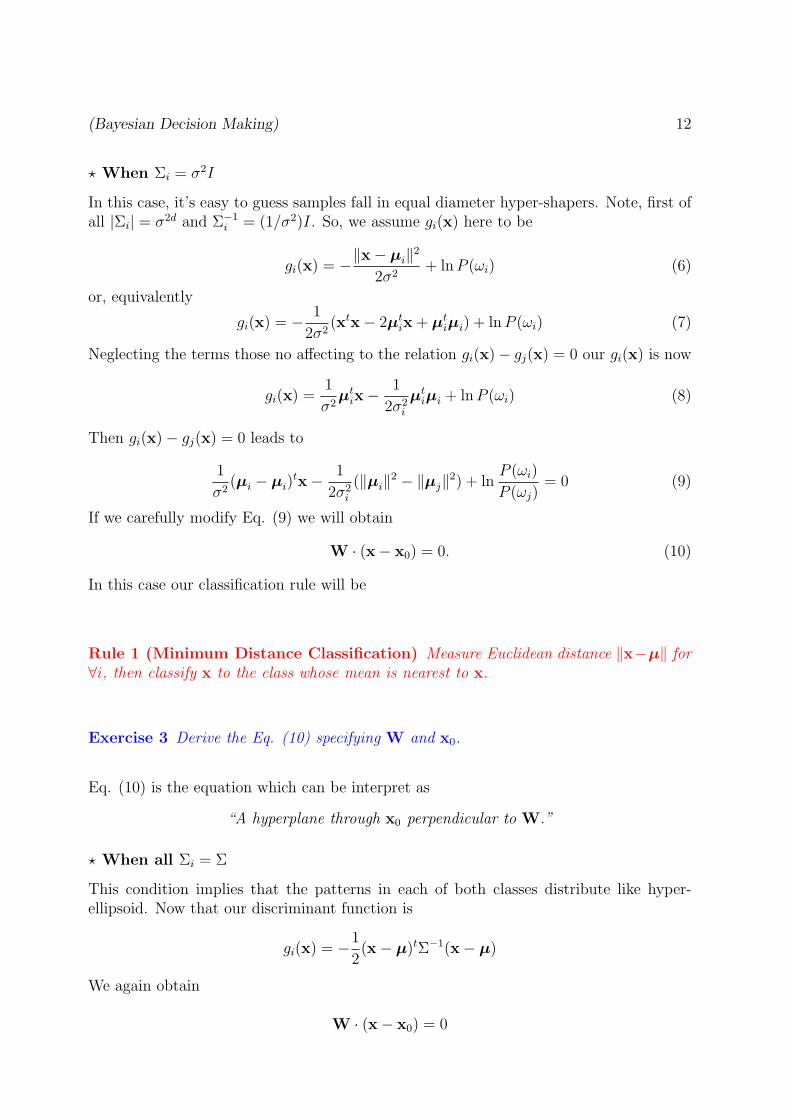
⋆ When Σi = σ2I
In this case, it’s easy to guess samples fall in equal diameter hyper-shapers. Note, first ofall |Σi| = σ2d and Σ−1
i = (1/σ2)I. So, we assume gi(x) here to be
gi(x) = −∥x− µi∥2
2σ2+ lnP (ωi) (6)
or, equivalently
gi(x) = − 1
2σ2(xtx− 2µt
ix+ µtiµi) + lnP (ωi) (7)
Neglecting the terms those no affecting to the relation gi(x)− gj(x) = 0 our gi(x) is now
gi(x) =1
σ2µt
ix− 1
2σ2i
µtiµi + lnP (ωi) (8)
Then gi(x)− gj(x) = 0 leads to
1
σ2(µi − µi)
tx− 1
2σ2i
(∥µi∥2 − ∥µj∥2) + lnP (ωi)
P (ωj)= 0 (9)
If we carefully modify Eq. (9) we will obtain
W · (x− x0) = 0. (10)
In this case our classification rule will be
Rule 1 (Minimum Distance Classification) Measure Euclidean distance ∥x−µ∥ for∀i, then classify x to the class whose mean is nearest to x.
Exercise 3 Derive the Eq. (10) specifying W and x0.
Eq. (10) is the equation which can be interpret as
“A hyperplane through x0 perpendicular to W.”
⋆ When all Σi = Σ
This condition implies that the patterns in each of both classes distribute like hyper-ellipsoid. Now that our discriminant function is
gi(x) = −1
2(x− µ)tΣ−1(x− µ)
We again obtain
W · (x− x0) = 0

(Bayesian Decision Making) 13
where W and x0 are
W = Σ−1(µi − µj) (11)
and
x0 =1
2(µi + µj)−
lnP (ωi)/P (ωj)
(µi − µj)tΣ−1(µi − µj)
(12)
Notice here that W is no more perpendicular to the direction between µi and µj.
Exercise 4 Derive w and x0 above.
So we modify the above rule to
Rule 2 (Classification by Mahalanobis distance) Assign x to ωi in which Maha-lanobis distance from µi is minimum for ∀i.
Yes! This Mahalanobis distance between a and b is defined as
(a− b)tΣ−1(a− b) (13)
• 3-D Gaussian case as an example
⋆ When all Σi = ΣHere we study only one example. We assume two classes where P (ω1) = P (ω1) = 1/2. Ineach class, the patterns are distributed with Gaussian p.d.f both have the same covariancematrix
Σi = Σj = Σ =
0.3 0.1 0.10.1 0.3 −0.10.1 −0.1 0.3
and means of the distribution are (0, 0, 0)T and (1, 1, 1)T . We now take a look at whatour discriminant function
gi(x) = −1
2(x− µi)
TΣ−1i (x− µi) (14)
leads to?
Since we calculate (See APPENDIX for detail)
Σ−1 =1
30
5 −3 −3−2 6 3−1 3 6

(Bayesian Decision Making) 14
Now our discriminant equation g1(x) = g2(x) is
(x1x2x3)
5 −3 −3−2 6 3−1 3 6
x1
x2
x3
=
((x1 − 1)(x2 − 1)(x3 − 1))
5 −3 −3−2 6 3−1 3 6
x1 − 1x2 − 1x3 − 1
Further calculation leads to
((5x1 − 2x2 − x3)(−3x1 + 6x2 + 3x3))
x1
x2
x3
=
((5x1 − 2x2 − x3 − 2)(−3x1 + 6x2 + 3x3 − 6)(−3x1 + 3x2 + 6x3 − 6))
x1 − 1x2 − 1x3 − 1
All the 2nd-order terms are canceled and we obtain,
7x1 + 13x2 − 20x3 = 14
We now know that it is the plane which discriminates two of these classes ω1 and ω2.

(Bayesian Decision Making) 15
PART IIBAYESIAN NETWORK
3 Bayesian Network
So far our conditional probabilities are sometimes probability distribution function, suchas p(x|ω), not a numerical value of probability. From now on, all the notations will benumerical value of the probability of some event. E.g. p(A|B) means the probability ofA under the condition of B, or equivalently, the probability of A given B. Specifically wecall them (A and B here) variables.
Then Bayesian network is a graph which represent dependence of these variables. Nodesrepresent these variables, and arcs represent the probability of these dependencies. Thatis, the arc from node A to B is p(B|A).
The objective of the Bayesian network is to infer a probability of some variable whoseprobability is unknown from the information of a set of value of the other variables. Theformer variable is called hypothesis and the latter are called evidences. Hence we may saythis objective is to:
Infer the probability of hypotheses from evidences given.
So our most frequent notation of a probability will be described p(h|e). Sometimes thisprobability is called belief and also described as
Bel(h|e).To simply put, this is, ”how much is our belief for the hypothesis given those evidences.”
3.1 Examples
3.1.1 Flu & Temperature
This example is taken from Korb et al.1
Flu causes a high temperature by and large. We now suppose the probability that weare flu is p(Flu) = 0.05, the probability that we have High-temperature when we are fluis p(High-temperature|Flu) = 0.9 and the probability of we still have a high temperatureeven when we are not flu (false alarm) is p(High-temperature|¬Flu) = 0.2. See Figure 2.
Exercise 5 Now we assume to have an evidence that one guy has a high-temperature,then how much is a belief of this guy is Flu?
1K. B. Korb and A. E. Nicholson (2003) ”Bayesian Artificial Intelligence.”

(Bayesian Decision Making) 16
Or conversely,
Exercise 6 We have an evidence that one guy is flu then how much is a belief of this guyhas a high-temperature?
Flu
High-temperature
FluF
HighTempF TFlu
FT
0.95
0.900.200.800.10
T
0.05
Figure 2: Flu causes high-temperature. Redrawn from Korb et al. (Sorry but withoutpermission.)
3.1.2 Season & Rain
In the example of the previous subsection, all the variables take a binary value. Sometimeswe want variables which takes more cases. Here we have such an example. Again a simpleexample of two variables but one is about season which takes 4 values: {winter, spring,summer and autumn}, and weather which takes also 4 values: {fine, cloudy, rain, andsnow} See Figure 3.
Season
Weather
A:
B:
a1a2a3a4
: winter: spring: summer: autumn
b1b2b3
: fine: cloudy: rain
b4 : snow
0.40.20.10.3
p(a)
p(b|a)
a1a2a3a4
b3 b4b1 b2
0.45 0.38 0.26 0.130.60 0.34 0.12 0.000.35 0.22 0.40 0.16
0.15 0.32 0.17 0.50
a1a2a3a4
Figure 3: Season & Weather
Now try the following two inferences. The first one is very direct.

(Bayesian Decision Making) 17
Exercise 7 Assume it’s now Summer (evidence), then how much is the probability thatit’s rain?
The next one is not such straight forward but still quite easy.
Exercise 8 Now it’s snow, then how much is the probability of being autumn now?
3.1.3 Flu, Temperature & Thermometer
Now we move on to a case of three variables. First one is simple enough like A → B → C.Let’s call A ”parent of B,” and C ”child of B.” This example is again taken from Korbet al.
Relation of Flu & High Temperature is the same as before. Now we have a thermometerwhose rate of false negative reading is 5% and false positive reading is 14 %, that is,
p(HighTherm = True|HighTemp = True) = 0.95p(HighTherm = True|HighTemp = False) = 0.15
Flu
High-temperature
FluF
HighTempF TFlu
FT
0.95
0.900.200.800.10
T
0.05
Thermometer-highHighTemp
F TThermoHigh
FT 0.05
0.150.850.95
Figure 4: Flu → HighTemp → ThermoHigh. Redrawn from Korb et al. (Sorry butwithout permission.)
Exercise 9 Evidence now is, he is Flu and Thermometer suggests HighTemp, then howmuch is the probability of hypothesis that he has a High temperature?
Or, lack of one evidence
Exercise 10 Now thermometer suggests HighTmp, then how much is the probability ofhis being Flu?

(Bayesian Decision Making) 18
3.1.4 Grass are soaked then it’s rain or sprinkler
Now we proceed a more complicated case in which dependency is not linear. This exampleis taken from Wikipedia.2
The situation is described in the page as:
Suppose that there are two events which could cause grass to be wet: either thesprinkler is on or it’s raining. Also, suppose that the rain has a direct effecton the use of the sprinkler (namely that when it rains, the sprinkler is usuallynot turned on). All three variables have two possible values, T for true and Ffor false.
Sprinkler
Grass-soaked
Rain
RAINT F0.2 0.8
SPRINKLERF T
Rain
FT
0.60 0.400.99 0.01
GRASS SOAKEDF TSPRINKLER RAIN
F F
F T
T F
T T
1.00 0.00
0.20 0.80
0.10 0.90
0.01 0.99
Figure 5: Grass are soaked because it’s rain and/or sprinkler?
Let’s calculate the joint probability function. First, recall that the joint probability of Aand B, in general, can be expressed as:
3.1.5 Pearl’s earthquake Bayesian Network
This is a very popular example to show how Bayesian network looks like by Pearl.3
You have a new burglar alarm installed. It reliably detects burglary, but alsoresponds to minor earthquakes. Two neighbors, John and Mary, promise tocall the police when they hear the alarm. John always calls when he hearsthe alarm, but sometimes confuses the alarm with the phone ringing and callsthen also. On the other hand, Mary likes loud music and sometimes doesn’thear the alarm. Given evidence about who has and hasn’t called, you’d like toestimate the probability of a burglary.
2at http : //en.wikipedia.org/wiki/Bayesian network3Pearl, J. (1988) ”Probabilistic Reasoning in Intelligent Systems: Networks of Plausible Inference.”
San Mateo, Morgan Kaufmann.
(Bayesian Decision Making) 19
Burglary
Alarm
Earthquake
JohnCalls MaryCalls
Burglary EarthquakeTF
0.010.99
TF
0.020.98
JohnCalls MaryCallsAlarm Alarm
TF
TF
0.700.01
0.300.99
TF
TF
0.900.05
0.100.95
Burglary
TF
Earthquake
FFTFFTTT
AlarmTF
0.999 0.0010.710 0.2900.060 0.9400.050 0.950
Figure 6: Pearl’s Earthquake
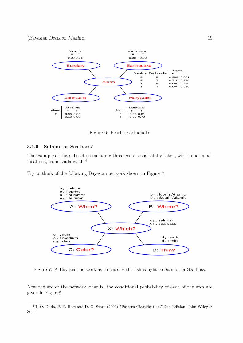
3.1.6 Salmon or Sea-bass?
The example of this subsection including three exercises is totally taken, with minor mod-ifications, from Duda et al. 4
Try to think of the following Bayesian network shown in Figure 7
When?
Which?
Where?
Color? Thin?
A: B:
X:
D:C:
a1a2a3a4
: winter: spring: summer: autumn
b1b2
: North Atlantic: South Atlantic
x 1x 2
: salmon: sea bass
d1d2
: wide: thin
c 1c 2c 3
: light: medium: dark
Figure 7: A Bayesian network as to classify the fish caught to Salmon or Sea-bass.
Now the arc of the network, that is, the conditional probability of each of the arcs aregiven in Figure8.
4R. O. Duda, P. E. Hart and D. G. Stork (2000) ”Pattern Classification.” 2nd Edition, John Wiley &Sons.
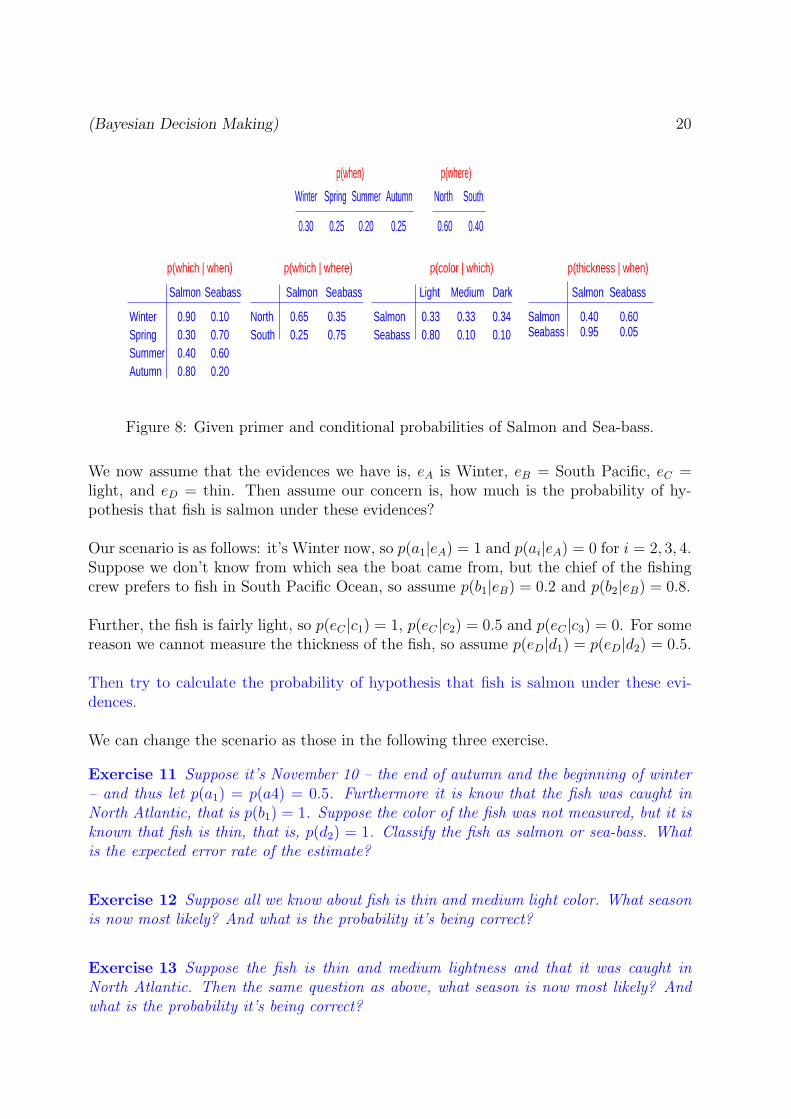
(Bayesian Decision Making) 20
Winter Spring Summer Autumn
p(when)
North South
0.60 0.40
p(where)
0.25 0.250.30 0.20
Salmon Seabass
WinterSpringSummerAutumn
p(which | when)
0.900.300.400.80
0.100.700.600.20
NorthSouth
0.650.25
0.350.75
p(which | where)
0.400.95
0.600.05
p(thickness | when)
Salmon Seabass
0.330.80
0.330.10
p(color | which)
SalmonSeabass
Light Medium Dark
0.340.10
SalmonSeabass
Salmon Seabass
Figure 8: Given primer and conditional probabilities of Salmon and Sea-bass.
We now assume that the evidences we have is, eA is Winter, eB = South Pacific, eC =light, and eD = thin. Then assume our concern is, how much is the probability of hy-pothesis that fish is salmon under these evidences?
Our scenario is as follows: it’s Winter now, so p(a1|eA) = 1 and p(ai|eA) = 0 for i = 2, 3, 4.Suppose we don’t know from which sea the boat came from, but the chief of the fishingcrew prefers to fish in South Pacific Ocean, so assume p(b1|eB) = 0.2 and p(b2|eB) = 0.8.
Further, the fish is fairly light, so p(eC |c1) = 1, p(eC |c2) = 0.5 and p(eC |c3) = 0. For somereason we cannot measure the thickness of the fish, so assume p(eD|d1) = p(eD|d2) = 0.5.
Then try to calculate the probability of hypothesis that fish is salmon under these evi-dences.
We can change the scenario as those in the following three exercise.
Exercise 11 Suppose it’s November 10 – the end of autumn and the beginning of winter– and thus let p(a1) = p(a4) = 0.5. Furthermore it is know that the fish was caught inNorth Atlantic, that is p(b1) = 1. Suppose the color of the fish was not measured, but it isknown that fish is thin, that is, p(d2) = 1. Classify the fish as salmon or sea-bass. Whatis the expected error rate of the estimate?
Exercise 12 Suppose all we know about fish is thin and medium light color. What seasonis now most likely? And what is the probability it’s being correct?
Exercise 13 Suppose the fish is thin and medium lightness and that it was caught inNorth Atlantic. Then the same question as above, what season is now most likely? Andwhat is the probability it’s being correct?

(Bayesian Decision Making) 21
3.2 A formula for inference
Recall a basic formula in probability theory named joint probability
Rule 3 (Joint Probability) Assuming we have n nodes of variables X1, X2, · · · , Xn.Then we can calculate the joint probability of X1, X2, · · · , Xn.
p(X1, X2, · · · , Xn) = Πni=1p(Xi|parent(Xi))
where Parent(X) means parent node of X.
See the following examples.
F
B
T
S
G
X
Y
Z
W
W
p(F,B,T)
=p(F)p(B|F)p(T|B)
p(W,S,G)
=p(W)p(S|W)p(G|W,G)
p(X,Y,Z,W)
=p(X)p(W)p(Y|X)pZ(Y,W)
Let’s try more challenging examples.
E
A
M
p(B,E,A,J,M)
=p(B)p(E)p(A|B,E)p(J|A|B)p(M|A)
p(W,S,C,I)
=p(W)p(S|W)p(C|W)p(I|S,C)
B
J
CS
W
I
CS
I
DW
p(W,D,S,C,I)
=p(W)p(D)p(S|W)p(C|W,D)p(I|S,C)
Exercise 14 Then what about the following example?
ED
CB
G
A
H
F

(Bayesian Decision Making) 22
How to calculate the probability of hypotheses given evidences?
Now question is, wow we calculate the probability of hypotheses given evidences? Assumewe have 5 variables A, B, C, D, and E, of which D = d is hypotheses, and A = a, andE = e are evidences, just an example. Then what we want to calculate is:
p(D = d|A = a,E = e).
A basic formula of probability tells us:
p(X, Y ) = p(X|Y )p(Y ).5
So,
p(X|Y ) =p(X,Y )
p(Y ).
Hence
p(D = d|A = a,E = e) =p(A = a,D = d,E = e)
p(A = a,E = e).
Then,
p(A = a,D = d,E = e) =∑B,C
p(A,B,C,D,E).
As we already obtained p(A,B,C,D,E) we can calculate this. And similarly,
p(A = a,E = e) =∑B,C,D
p(A,B,C,D,E),
where, for example, ∑B,C,D
p(A,B,C,D,E)
means sum over all possible value of B, C, and D while remain A = a and E = e. Now letus take a further concrete example Weather-Sprinkler-GrassWet where we have alreadylearned
p(R,S,G) = p(R)p(S|R)p(G|S,R).
Assume now we want to know the probability of hypotheses ”It’s rain” under the evidenceof ”Grass is wet,” for example. Then
p(R = true|G = true) =p(R = true,G = true)
p(G = true)=
∑S p(R = true, S,G = true)∑
R,S p(R, S,G = true)
For the sake of simplicity, let’s denote p(R = true, S = true,G = true) = TTT , p(R =true, S = true,G = false) = TTF , p(R = false, S = false,G = true) = FFT , and soon, then the above equation can be described as
=TTT + TFT
TTT + TTF + TFT + TFF
Now we can calculate the probability value, can we not?
5or, p(X,Y ) = p(Y |X)p(X) depending on the situation.

(Bayesian Decision Making) 23
4 Bayesian network for decision making
4.1 Utility
When we make a decision of an action, we might consider our preferences among differentpossible outcomes of those available actions. In the Bayesian decision theory this pref-erence is called utility, or we may rephrase it as ”usefulness,” ”desirability,” or simply”value” of the outcome.
Introducing this concept of utility allows us to calculate which action is expected to resultin the most valuable utility given any available evidence E.
We now define expected utility as:
eu(A|E) = p(Oi|E,A)u(Oi|A),
where A is an action with possible outcome Oi. E is the available evidence. U(Oi)|Ais the utility of each of the outcome under the action A. p(Oi|E,A) is the conditionalprobability distribution over the outcome Oi under the action A with the evidence E. Eis the available evidence.
4.1.1 Three different nodes to express network
• Chance nodes
• Decision nodes:
– The decision being made at a particular point in time. The values of a decisionnode are the actions
• Utility nodes:
– Each utility node has an associated utility table with one entry for each possibleinstantiation of its parents, perhaps including an When there are multipleutility nodes, the overall utility is the sum of the individual utilities.
Chance Decision Utility (value)
Figure 9: Symbol to express BDN – Chance, Decision, and Utility

(Bayesian Decision Making) 24
4.2 Example-1: To bet or not to my football team?
Clares football team, Melbourne, is going to play her friend Johns team, Carl-ton. John offers Clare a friendly bet: whoevers team loses will buy the winenext time they go out for dinner. They never spend more than $15 on winewhen they eat out. When deciding whether to accept this bet, Clare will have toassess her teams chances of winning (which will vary according to the weatheron the day). She also knows that she will be happy if her team wins andmiserable if her team loses, regardless of the bet.
Weather
Result
Accept Bet
How Happy?
Weatherdry wet0.7 0.3
weathermy team win
0.60
F T
0.250.400.75
Result Accept Bet
no -5drywet
How Happy?
lostyes -20lostno 20winyes 40win
Figure 10: To bet or not to my football team?
Algorithm 1 Decision network evaluation with a single decision node:
1. For each action value in the decision node:
(a) Set the decision node to that value;
(b) Calculate the probability for the parent nodes of the utility node;
(c) Estimate the utility for the action by selecting variables one by one from theseparent nodes: such that if the variable is evidence then select it, otherwise thehighest probability variable in the current node. From the utility table, We candecide the most favorable action for these selected variables of the parent nodes.
2. Return the action.

(Bayesian Decision Making) 25
4.2.1 Information links
There may be arcs from chance nodes to decision nodes these are called information links.
Weather
Result
Accept Bet
How Happy?Forecast
Information link
Weahter
Forecast
rainy cloudy sunny
wet
dry
0.60 0.25 0.15
0.10 0.40 0.50
Forecast Accept Betrainy
cloudy
sunny
yes
no
no
Decision Table
Figure 11: An example of information link.
Algorithm 2 Decision network evaluation with multiple decision nodes:
1. For each combination of values of the parents of decision node:
(a) For each action value in the decision node:
i Set the decision node to that action.
ii Calculate the posterior probabilities for each of the parent nodes of theutility node from one parent node to the next.
iii Record the utility value corresponding to the combination of the highestprobability set of parent nodes of the utility node calculated in (ii).
(b) Record the action with the highest utility value for the action in the decisiontable.
3. Return the decision table.
4.2.2 An example of decision making table
(Allow me to skip this.)

(Bayesian Decision Making) 26
4.3 Sequential decision making
4.3.1 Revisit to the Flu example
Suppose that you know that a fever can be caused by the flu. You can use athermometer, which is fairly reliable, to test whether or not you have a fever.Suppose you also know that if you take aspirin it will almost certainly lowera fever to normal. Some people (about 5% of the population) have a negativereaction to aspirin. You’ll be happy to get rid of your fever, as long as youdon’t suffer an adverse reaction if you take aspirin.
F
Flu
Fever
Take Aspirin
meritThermo
Fever LaterBad Reaction
information link
F T0.95 0.05
Fever
Flu T
TF 0.02
0.950.05
0.98
Flu
FeverF T
0.05
0.900.10
0.95TF
ThermoFever Take Aspirin
Fever Later
F noF T
0.020.98F yes 0.010.99T no 0.900.10T yes 0.050.95
F
Bad Reaction
Take Aspirin T
T0.020.950.05
0.98F
Fever Later Bad Reaction merit
F no -50F yes -10T no -30T yes 50
Figure 12:
4.3.2 An investment to a Real estate
Paul is thinking about buying a house as an investment. While it looks fineexternally, he knows that there may be structural and other problems with thehouse that aren’t immediately obvious. He estimates that there is a 70% chancethat the house is really in good condition, with a 30% chance that it could bea real dud. Paul plans to resell the house after doing some renovation. Heestimates that if the house really is in good condition (i.e., structurally sound),he should make a $5,000 profit, but if it isn’t, he will lose about $3,000 onthe investment. Paul knows that he can get a building surveyor to do a fullinspection for $600. He also knows that the inspection report may not becompletely accurate. Paul has to decide whether it is worth it to have thebuilding inspection done, and then he will decide whether or not to buy thehouse.

(Bayesian Decision Making) 27
Report
Condition
Buy
How Happy?Inspect
Good?
Inspect Good?no
yes -6000
Condition
goodbad 0.3
0.7
Buy Condition How Happy?no bad 0no good 0yes bad -3000yes good 5000
Inspect ConditionReport
no bad
bad unknown good
no goodyes badyes good
0.00 1.00 0.000.00 1.00 0.000.90 0.00 0.100.05 0.00 0.95
Figure 13: Revised real-estate example.
4.4 Dynamic Bayesian network (DBN)
When we say Bayesian network, usually all events are static. In other words, all theprobability value do not change as time goes by. But as we see in the Flu-Fever-Aspirinexample above, taking an aspirin influence the fever tomorrow. Now we study the prob-abilities are dynamically change as a function of time with the structure of the networkbasically remaining the same. The structure of the network at time t is called a time-slice.Arcs in one time-slice is called inter-slice arcs while arcs link to the next time-slice arecalled intra-slice arcs.
Intra-slice are usually not from all the nodes to the corresponding nodes in the next time-slice. Only sometimes we have such connections as Xi(T ) → Xi(t+1). Or sometimes onenode in one time-slice links different node in the next time-slice Xi(T ) → Xj(t+ 1).
Flu
Fever
Thermometer-high
Flu
Fever
Thermometer-high
p(Flu_after | Flu_before)
p(Feaver_after | Feaver_before)
Figure 14: Revised Flu example as a simple case of Dynamic Bayesian Network.

(Bayesian Decision Making) 28
Sometimes some nodes wield an observation, and as a result we see a time series ofobservation. In this scenario the node that wields the observation is called state.
Reaction
Take aspirine
Flu
Fever
Thermo
Reaction
Take aspirine
Flu
Fever
Thermo
U
t t+1
Figure 15: Still simple but more realistic Dynamic Bayesian Network.
Sometimes we want to call a node which creates an result that we can observe. Fromthe other field like a Model of Automaton or the Hidden Markov Model, it might beconvenient to call such nodes state and observation.
state
observation
Figure 16: Node ”state” and node ”observation”
Such Dynamic Bayesian Network are useful when we must make a decision making inan uncertainty. That is to say, it’s a good tool for Sequential design making or planningunder uncertainty. Let’s recall the example of decision making: to take an aspirin or notto take being afraid of it bad reaction to a body.
4.4.1 Mobile robot example
We now assume a mobile robot whose task is to detect and chase a moving object. Therobot should reassess its own position as well as the information where the target objectis. The robot observes at any slice of time its position with respect to walls and cornersand the target position with respect to the robot.

(Bayesian Decision Making) 29
state
observation
state
observation
U
Decision Decision
tt-1
D t such that maximizeU
Figure 17: A Dynamic Bayesian Network for decision making.
We denote the real location of own and target at time t as ST (t) and SR(t), and theobservation of location of own and target at time t as OT (t) and OR(t). Utility is thedistance from own to target.
S T
OTOR
S R
U
M
S T
OTOR
S R
U
M
Figure 18: Dynamic Bayesian Network for a mobile robot.

(Bayesian Decision Making) 30
CONCLUDING REMARKS
In the article in The New York Times on 16 March 2012, Steve Lohr wrote:
Google search, I.B.M.’s Watson Jeopardy-winning computer, credit-card fraud de-tection and automated speech recognition. There seems not much in common on thatlist. But it is a representative sampling of the kinds of modern computing choresthat use the ideas and technology developed by Judea Pearl, the winner of this year’sTuring Award. The award, often considered the computer science equivalent of aNobel prize, was announced on Wednesday by the Association for Computing Ma-chinery. ”It allowed us to learn from the data rather than write down rules of logic,”said Peter Norvig, an artificial intelligence expert and research director at Google.”It really opened things up.”
Dr. Pearl, with his work, he added, ”was influential in getting me, and many oth-ers, to adopt this probabilistic point of view.” Dr. Pearl, 75, a professor at theUniversity of California, Los Angeles, is being honored for his contributions to thedevelopment of artificial intelligence. In the 1970s and 1980s, the dominant ap-proach to artificial intelligence was to try to capture the process of human judgmentin rules a computer could use. They were called rules-based expert systems. Dr.Pearl championed a different approach of letting computers calculate probable out-comes and answers. It helped shift the pursuit of artificial intelligence onto morefavorable terrain for computing. Dr. Pearl’s work on Bayesian networks - named forthe 18th-century English mathematician Thomas Bayes - provided ”a basic calculusfor reasoning with uncertain information, which is everywhere in the real world,”said Stuart Russell, a professor of computer science at the University of California,Berkeley. ”That was a very big step for artificial intelligence.”
Dr. Pearl said he was not surprised that his ideas are seen in many computingapplications. ”The applications are everywhere, because uncertainty is everywhere,”Dr. Pearl said. ”But I didn’t do the applications,” he continued. ”I provided a wayfor thinking about your problem, and the formalism and framework for how to do it.”
(The Turing Award, named for the English mathematician Alan M. Turing, includes
a cash prize of $250,000, with financial support from Intel and Google.)

(Bayesian Decision Making) 31
APPENDIX
I. Quadratic form in 2-dimensional space
You might be interested, first of all, in how points scattered are influenced by values inΣ, that is, σ2
1, σ22, and σ12 = σ21. Let’s observe here three different cases of Σ when
µ = (0, 0).
(1) Σ1 =
(0.20 00 0.20
)(2) Σ2 =
(0.1 00 0.9
)(3) Σ3 =
(0.5 0.30.3 0.2
)
-4
-3
-2
-1
0
1
2
3
4
-4 -3 -2 -1 0 1 2 3 4
’sigma-2-0-2-0.data’
-4
-3
-2
-1
0
1
2
3
4
-4 -3 -2 -1 0 1 2 3 4
’sigma-1-0-9-0.data’
-4
-3
-2
-1
0
1
2
3
4
-4 -3 -2 -1 0 1 2 3 4
’sigma-5-3-3-2.data’
Figure 19: A cloud of 200 Gaussian random points with three different three Σ.

(Bayesian Decision Making) 32
II. How to calculate inverse of 3-dimensional matrix.
We now try to calculate the inverse of the following 3-D matrix A which appeared in thesubsection ??.
A =
0.3 0.1 0.10.1 0.3 −0.10.1 −0.1 0.3
We use a relation Ax = I where x = (x, y, z)T and I is identity matrix, i.e., 0.3 0.1 0.1
0.1 0.3 −0.10.1 −0.1 0.3
xyz
=
1 0 00 1 00 0 1
It remains identical if we multiply {2nd-raw} by 3 and subtract the {1st-raw}, i.e., 0.3 0.1 0.1
0 0.8 −0.40.1 −0.1 0.3
xyz
=
1 0 0−1 3 00 0 1
In the same way, but this time, we multiply {3rd-raw} by 3 and subtract the {1st-raw}. 0.3 0.1 0.1
0 0.8 −0.40 −0.4 0.8
xyz
=
1 0 0−1 3 0−1 0 3
Then, e.g., multiply the {1st-raw} by 8 and then subtract the {2nd-raw}: 2.4 0 1.2
0 0.8 −0.40 −0.4 0.8
xyz
=
9 −3 0−1 3 00 0 3
Multiply the {3rd-raw} by 2 and then add the {2nd-raw}: 2.4 0 1.2
0 0.8 −0.40 0 1.2
xyz
=
9 −3 0−1 3 0−1 3 6
Subtract {3rd-raw} from the {1st-raw}: 2.4 0 0
0 0.8 −0.40 0 1.2
xyz
=
10 −6 −6−1 3 0−1 3 6
Multiply the {2nd-raw} by 3 then add the {3rd-raw}: 2.4 0 0
0 2.4 00 0 1.2
xyz
=
10 −6 −6−4 12 6−1 3 6

(Bayesian Decision Making) 33
Finally, divide the {1st-raw} by 2.4, divide the {2nd-raw} by 2.4, and divide the {3rd-raw}by 1.2, we obtain,
1 0 00 1 00 0 1
xyz
=1
30
5 −3 −3−2 6 3−1 3 6
Now we know the right-hand-side is the inverse of A because the equation implies Ix = Band it holds AIx = AB, that is, Ax = AB. Hence AB = I which means B = A−1.
To make it sure, calculate and find
0.3 0.1 0.10.1 0.3 −0.10.1 −0.1 0.3
× 1
30
5 −3 −3−2 6 3−1 3 6
=1
6
25 −15 −15−10 30 15−5 15 30
×
0.3 0.1 0.10.1 0.3 −0.10.1 −0.1 0.3
=
1 0 00 1 00 0 1
Therefore
A−1 =1
30
5 −3 −3−2 6 3−1 3 6

![Bayes Decision Theory [Lecture]](https://static.fdocuments.in/doc/165x107/55cf885b55034664618fb762/bayes-decision-theory-lecture.jpg)