Back testing “The Magic Formula” in the Nordic region

STOCKHOLM SCHOOL OF ECONOMICS DEPARTMENT OF FINANCE MASTER THESIS 2009

Back testing “The Magic Formula” in the Nordic region

Victor Persson† & Niklas Selander††

ABSTRACT

We will in this thesis back test Joel Greenblatt’s magic formula on stocks in the Nordic Region between January 1st

1998 and January 1st

2008. We will compare the return with benchmarks such as MSCI Nordic and S&P 500 as well

as the return predicted by the Capital Assets Pricing Model (CAPM) and Fama French’s three factor model. The

portfolio based on the formula had during the ten year period a compounded annual growth rate (CAGR) of 14.68

percent compared to 9.28 percent for the MSCI Nordic and 4.23 percent for the S&P 500. However, the intercept

was not significant neither when testing against the CAPM or Fama French’s three factor model on the 5 percent

level. Adding transaction cost lowers the CAGR to 11.98 percent. With transaction costs, the intercepts were not

significant neither when testing against the CAPM or Fama French’s three factor model on the 5 percent level. The

Sharpe ratio for the portfolio was above MSCI Nordic and S&P 500 both with and without transaction costs. We

also find that the return of the portfolios improve when including intangible assets in the magic formula.

† [email protected] †† [email protected] TUTOR: Clas Bergström KEYWORDS: Efficient markets, Magic Formula, Joel Greenblatt ACKNOWLEDGEMENTS: We would first like to thank Professor Clas Bergström for his advices and guidance. We would also like to thank Pauline Nisha and Wilfred Wilson from Thomson regarding their invaluable help regarding the DataStream database.

i

Table of Contents

1 INTRODUCTION ..........................................................................................................................1

2 PREVIOUS RESEARCH ..................................................................................................................2

2.1 EFFICIENT MARKET HYPOTHESIS........................................................................................................... 2

2.2 FINDINGS CONTRADICTING THE EMH .................................................................................................... 3

2.2.1 Size effect .............................................................................................................................. 3

2.2.2 January effect ........................................................................................................................ 3

2.2.3 Weekend effect ..................................................................................................................... 4

2.2.4 Contrarian ............................................................................................................................. 5

2.2.5 Momentum ........................................................................................................................... 5

2.2.6 Ratios .................................................................................................................................... 6

3 GREENBLATT’S MAGIC FORMULA ................................................................................................7

3.1 INTRODUCTION ................................................................................................................................. 7

3.2 THE MAGIC FORMULA ........................................................................................................................ 7

3.2.1 Ranking ................................................................................................................................. 8

3.2.2 Results ................................................................................................................................... 9

3.2.3 Risk and investment time horizon ....................................................................................... 10

3.3 GREENBLATT VERSUS EFFICIENT MARKET HYPOTHESIS ............................................................................ 11

3.4 PREVIOUS BACK TESTING OF THE GREENBLATT’S WORK ......................................................................... 12

3.5 THE POSSIBILITY TO USE ANOMALIES AS TRADING STRATEGIES .................................................................. 15

3.6 THE ANOMALIES AND GREENBLATT ..................................................................................................... 16

4 METHOD AND DATA ................................................................................................................. 16

4.1 METHOD ........................................................................................................................................ 16

4.2 BAD MODEL PROBLEM AND THE JOINT HYPOTHESIS PROBLEM ................................................................. 20

4.3 DATA ............................................................................................................................................. 21

5 HYPOTHESIS ............................................................................................................................. 21

6 RESULTS ................................................................................................................................... 23

6.1 HYPOTHESIS 1 ................................................................................................................................. 23

6.2 HYPOTHESIS 2 ................................................................................................................................. 24

6.3 HYPOTHESIS 3 ................................................................................................................................. 25

6.4 HYPOTHESIS 4 ................................................................................................................................. 26

6.5 ADDING TRANSACTION COSTS ............................................................................................................ 27

6.6 ROLLING 12 MONTH PERFORMANCES ................................................................................................ 30

7 DISCUSSIONS AND CONCLUSIONS ............................................................................................. 30

ii

8 FURTHER RESEARCH ................................................................................................................. 31

9 REFERENCE LIST ........................................................................................................................ 32

9.1 ACADEMIC REFERENCES .................................................................................................................... 32

9.2 NON-ACADEMIC REFERENCES ............................................................................................................ 34

9.3 OTHER SOURCES .............................................................................................................................. 34

9.4 DATABASES .................................................................................................................................... 34

10 APPENDIX ............................................................................................................................. 35

10.1 MORE OF GREENBLATT’S RESULTS ...................................................................................................... 35

10.2 ROLLING 12 MONTH PERFORMANCE .................................................................................................. 36

10.3 THE CASE OF RAYSEARCH LABORATORIES ............................................................................................ 37

10.4 ORIGINAL LIST OF STOCK................................................................................................................... 41

10.5 THE STOCKS SELECTED IN EACH PERIOD .............................................................................................. 55

10.6 RESULT IN EACH PERIOD ................................................................................................................... 61

10.7 SUMMARY OUTPUT OF REGRESSIONS .................................................................................................. 62

1

1 Introduction

Can you beat the market? Or rather, can you systematically beat the stock market taking advantage of

market inefficiency? This is a frequently debated question within academic circles as well as among

practitioners in the investment community. Supporters of the Efficient market hypothesis (EMH) claim

that you cannot, while others argue that you can. Investors systematically outperforming the market

have been present during many decades, including; John Templeton, Warren Buffet and Peter Lynch.

We will in this thesis examine a trading strategy from the perspective of EMH. The trading strategy that

we have chosen is the strategy presented by hedge fund manager and adjunct professor Joel Greenblatt

in his bestselling book The little book that beats the market.

Since the efficient market hypothesis became widely accepted in the academic world in the 1970s

(Schiller (2003)), many attempts have been done to show its flaws. We will highlight some of the

anomalies that have been found, and to large extent disappeared, during the years. Some of the

anomalies are more interesting in the understanding of our study, explaining the reason for us to

penetrate deeper into those1. We will summarize these anomalies and give our current view on their

implications on investment strategies in general and Greenblatt’s strategy in particular.

Can you beat the market with approximately 10 percent per year for decades without additional risk?

Well, Joel Greenblatt claims this is in his book The little book that beats the market. Greenblatt’s book

has gained attention within the investment community and his strategy has been successfully back-

tested and published by e.g. Lancetti and Montier for Dresdner Kleinwort Wasserstein (DrKW), and by

Robert Haugen, professor in finance at UCLA at Irvine.

Greenblatt belongs to the investment philosophy called Value investing. Value investing has a long

history, dating back to the work by Benjamin Graham and David Dodd in their book Security Analysis

from 1934, and further developed by Graham in the book The intelligent Investor from 1949. The value

investing community, including Greenblatt, has a different view of risk compared to supporters of EMH.

Greenblatt and most other value investors disagree on volatility being the proper measure for risk,

arguing that the fact that volatility “punishes” upside volatility with increased risk is wrong (Dremen

(1998), Greenblatt (2006), Greenwald et al. (2001)). They believe risk to be the probability of losing

1 Some of the anomalies are included for illustrative purposes.

2

money and protect themselves against that via thorough analysis and margin of safety2. Since the value

investing community has a different view of risk, we believe it would be interesting to examine

Greenblatt’s strategy through a more traditional and academic view of risk via asset pricing models.

The contribution of this thesis is aimed to be fivefold. Firstly, we will try to put Greenblatt’s method in a

perspective using previous research regarding EMH. Secondly, we will test Greenblatt’s formula on

Nordic stocks. To our knowledge this has not been done before. Thirdly, we will test Greenblatt’s

method against two asset-pricing models – the CAPM and Fama & French’s three-factor model - to see if

the method produces abnormal return. That is also something that to our knowledge has not been done

before. Fourthly, we will also test a portfolio including intangible assets and see if that affect the

performance of the formula. Finally, we will try to conclude whether the magic formula is a good

investment strategy or not.

2 Previous Research

2.1 Efficient Market Hypothesis According to Fama (1970), a market in which prices always fully reflect available information is a

efficient market. Jensen (1978) later developed a definition of efficient market as a market where it is

impossible to make economic profits3 by trading on a certain set of information.

Fama (1970) developed three forms of the efficient market hypothesis (EMH): weak form, semi-strong

form and strong form. In the weak form, current prices reflect all information obtainable by examining

historical prices, meaning that technical analysis will not lead to abnormal returns, while fundamental

analysis may. The semi-strong form maintains that prices reflect all public available information, e.g.

earnings announcements and annual reports. According to this, neither technical- nor fundamental

analysis will lead to abnormal returns. Finally, in strong form, prices fully reflect both public and private

information and thus, not even investors with monopolistic access to information, e.g. insiders, will be

able to earn abnormal return. Fama (1970) conclude that empirical research supports both the weak-

and semi-strong form.

There has been a lot of support for EMH since Fama’s defintion. Until the mid-1980s empirical research

and theoretical reasoning vastly supported the EMH. Jensen (1978) even went so far as saying that there

2 Value Investors do typically not invest in what they believe to be fair value. They want a margin of safety as well

to give them downside protection. 3 By economic profit, Jensen means risk-adjusted return net all costs.

3

is no other proposition in economics that has a more solid empirical support than the EMH. Implications

of the EMH dominance in the field of investment were seen, as index-funds and buy-and-hold strategies

became increasingly popular (Szyszka (2007)).

2.2 Findings contradicting the EMH Empirical studies that find patterns contradicting the EMH are numerous, though most of them have

disappeared. Some of these anomalies, as they are called by EMH supporters, have been tried to be

explained by what is called behavioral finance – finance from a psychological and social perspective

(Schiller (2003)). Contrasting the classical paradigm of EMH, behavioral finance assumes that investors

are not always rational in their reactions to market information (Szyszka (2007)). Since there have been

extensive research performed regarding EMH, we will in this thesis only give a brief introduction to the

effects and anomalies that caused the emergence of the field of behavioral finance in the mid 1980s and

1990s.

2.2.1 Size effect

Banz (1981) studied the relationship between return and the market value of common stocks. Banz

found that, for the period between 1936 and 1975, the stocks of small size firms had on average higher

risk-adjusted return4 than the stocks of large firms. This finding would be known as the size effect. Chan

and Chen (1991) found that size had reliable explanatory power on the distribution of returns among

the size portfolios. However, when adding additional risk factors, determined by the stock’s sensitivity

to a value-weighted index, a leverage index and a dividend-decrease index, size lost its explanatory

power. This suggests that there is a risk proxy captured by size and that is not captured by CAPM. More

recent studies suggest that the small-size effect has disappeared. For example, Horowitz et al (2000)

examine data for the period between 1982 and 1997 and they found no sign of a small-size effect.

2.2.2 January effect

Keim (1983) argues that the studies by Banz (1981) implicitly assume that size-related excess returns are

obtained continuously; i.e. evenly throughout time. According to Keim’s findings, a significant

proportion of the size effect is due to the return premium observed during the month of January each

year.5 The average annual premium of 30.3 percent is reduced to 15.4 percent when the January

observations are removed, thus the exclusion of January-observations reduces the overall anomaly by

close to 50 percent. This finding would be known as the January effect.

4 Banz used CAPM to determinate the risk-adjusted return.

5 Test performed for the period (1963-1979).

4

Possible explanations of the January effect are proposed by e.g. Wachtel (1942) and Branch (1977),

explaining the abnormal returns with tax-loss selling of shares at the end of the year. Roll (1983)

suggests that the annual pattern in small firm returns is strongly associated with tax loss selling, and

suggest, in line with Lakonishok and Smidt (1984), that in the case of small firms, small trading volume

and large bid-ask spreads neutralize big profit opportunities (Thaler (1987)). Evidence suggests that

taxes may not be the only explanation of the January effect. In Great Britain and Australia, January

effects where identified by Thaler (1987) even though their tax years begin on other times a year. It

should be noted that returns in both countries are high in the beginning of the tax-year, indicating that

tax has implications on abnormal returns, but may not be the only explanation.

Another possible explanation is the information hypothesis. Keim (1983) states that January is a period

of increased uncertainty due to the release of important information. The distribution of this

information during January may have a greater impact on the prices of small firms, relative to large

firms, since the gathering and processing of information in small firms is a less costly process (Keim

(1983)).

2.2.3 Weekend effect

First reported by Cross (1973) and further developed by French (1980), the Monday effect, later to be

known as the Weekend effect, refers to the tendency of stocks to have relatively larger returns on

Fridays compared to Mondays. According to Dyl and Marbely (1988), common stocks and other financial

assets earn negative average returns on Mondays, because of the amount of unfavourable information

during the weekend. Dyl and Marbely (1988) further argue that this does not explain the anomaly, as

rational investors keep holding the financial assets during this unfavourable part of the week.

The Monday effect is perhaps the strongest of the calendar anomalies, despite this not large enough to

build a trading strategy around it (Rubenstein (2001)). According to Rubenstein (2001), while the U.S.

stock market rose with approximately 10 percent per year, the Friday-close to Monday-close return was

negative. In accordance with Rubenstein’s findings, Keim and Stambaugh (1984) add to the findings of

Cross (1973) and French (1980), that the majority of the negative average return on the S & P Composite

for the period 1928-1952, occurs during the non-trading period from Monday open to previous Friday

close, hereby stressing that the Monday effect in fact is a Weekend effect. The results are similar to the

ones reported by French (1980) for the period 1953-1977 and also supported by Rogalski (1984). The

5

latter also found empirical evidence of an inexplicable link between the Weekend effect, the January

effect and the size effect; small firms have higher return on Mondays in January than large firms.

Schwert (2003) found the estimate of the weekend effect not being reliably different from the other

days of the week since 1978. Sullivan, Timmerman and White (1999) showed that the effect could easily

be the result of data mining or chance. After 1987, the weekend effect has disappeared and more

strikingly, during the period 1989–1998 Monday has been the best day of the week, suggesting there is

no such thing as a weekend effect (Rubenstein (2001)).

2.2.4 Contrarian

De Bondt and Thaler (1985) used monthly data from 1926 to 1982 to form a winners’- and a losers’

portfolios based on the stocks’ past long-term performance6 and then measured the performance of the

stocks over the next three years. The result was that the losers earned 24.6 percent more than the

winners over the following three-year period, despite that the winners were significantly more risky.

According to these findings there is a contrarian effect, meaning that losers outperform winners in the

subsequent time period. De Bondt and Thaler (1985) explained their result with market overreactions to

unexpected news and information.

Chan (1988) argued that De Bondt’s and Thaler’s (1985) results were due to failure to risk-adjust returns.

Chan found that the risk of winners and losers were not constant. When adjusted for this, Chan only

found small abnormal returns, which were likely to be economically insignificant.

2.2.5 Momentum

In contrast to the contrarian effect, there is the momentum effect. Jegadeesh and Titman (1993) studied

data for the period between 1965 and 1989. Their strategy is based on buying stocks that have

performed well in the past 3- to 12-month period and sell stocks that have performed poorly in the

same period. Jegadeesh and Titman (1993) found that the strategy generated significant positive returns

over 3- to 12-month holding periods. They argue that the findings were not due to the strategy’s

systematic risk, nor to a delay in stock price reactions. Lo and MacKinlay (1988) examined weekly

returns of US stocks for the period 1962-1987, and found significant positive serial correlation in weekly

and monthly holding-period returns.

6 Ranging between one to five years

6

2.2.6 Ratios

2.2.6.1 Price-to-earnings (P/e)

Basu (1977) found empirical evidence of stocks with low P/e-ratios outperforming stocks with high P/e-

ratios, during the period April 1957-March 1971. The tests performed by Basu (1977) using; Jensen’s

alpha, Treynor- and Sharpe measures, show that low P/e-portfolios on average outperform random

portfolios of equivalent risk, while high P/e-portfolios fail to outperform randomly selected portfolios of

equivalent risk. All investors with the aim of rebalancing their portfolio annually (and tax-exempt

investors) could find abnormal returns. Transactions costs, search costs and tax effects prevented

traders7 from taking advantage of the market inefficiency. Basu’s findings implicate that security price

behavior is not consistent with the semi-strong form of the efficient market hypothesis. Basu suggests

there are exaggerated investor expectations on high P/e-stocks, and lags in new information being

accurately interpreted by investors. Chan, Hamao, and Lakonishok (1991) have found similar results.

Fama and French (1992) argue that low P/e-stocks are fundamentally riskier. Lakonishok, Shleifer and

Vishny (1994) on the other hand show that the reward for bearing fundamental risk does not explain

higher average returns on low P/e-stock portfolios.

2.2.6.2 Dividend-to-price (d/p)

As P/e, dividend yield or (d/p) is an initial value parameter that has been used extensively in empirical

research, in trying to determine future stock returns. The ratio d/p is simply the dividend divided with

the stock price. Fama and French (1988) and Campbell and Shiller (1988) have in found that a significant

portion of the variance of future returns for the stock market can be predicted by the initial dividend

yield. Furthermore, they show that investors have earned a higher rate of return from the stock market

when they purchased a market basket of equities with an initial dividend yield that was relatively high.

Fama and French (1988) argue that the stock returns are more predictable when measured over a

longer time period.

Fluck, Malkiel and Quandt (1997) found that a higher rate of return on equities with initially high

dividend yield is not consistent for individual stock picking. Investors purchasing a portfolio of individual

stocks with the highest dividend yields in the market will not earn a particularly high rate of return.

Examples of mutual funds pursuing this strategy underperformed the market during the period 1995-

1999, according to Malkiel (2003). Malkiel (2003) shows evidence of dividend yields being unable to

predict future returns since the mid-1980s. Fama and French (2001) argue that this may be due to a

7 Rebalancing more frequently.

7

changing pattern in dividend behavior of companies, using share buyback programs as means of pay out

money to shareholders. Thus, dividend yield may not be as meaningful as in the past as a predictor of

future equity returns.

3 Greenblatt’s Magic Formula

3.1 Introduction In an attempt to link the vast amount of theory on the field of investments to a more pragmatic view on

investments, we have chosen to further investigate the magic formula strategy presented by Joel

Greenblatt in his book The little book that beats the market.

Joel Greenblatt is a value investing hedge fund manager at Gotham Capital and adjunct professor at

Columbia University. Greenblatt summarizes his investment philosophy into a simple selection process

based on return on capital and earnings yield, both defined in his own way. Companies are ranked

according to these two selection criteria and investments are done in the companies with the best

combined rankings. This process makes up the magic formula, which will be treated in the next sections.

3.2 The Magic formula When valuing a company, Greenblatt stresses the fact that predictions and estimates are guesses of the

future outcomes, and those predictions are therefore flawed. The magic formula takes into account

factors that are known, making no predictions. In performing the ranking and building of an entire

portfolio of stocks, the best reasonable proxy publically available is, according to Greenblatt, last year’s

performance. The magic formula ranks companies based on two factors:

(i) Return on capital = EBIT8/ Tangible capital employed9

(ii) Earnings Yield = EBIT/ Enterprise Value10

Greenblatt’s way of defining Return on capital is by measuring the ratio of the 12 month trailing pre-tax

operating profits to tangible capital employed (Net Working Capital + Net Fixed Assets). He presents

several reasons for why he uses this ratio instead of the more common ROA (earnings/total assets) or

ROE (earnings/equity).

8 Earnings before Interest and Tax

9 Net Working Capital + Net Fixed Assets

10 Market value of equity (including preferred equity) + net interest bearing debt + minority interest

8

EBIT is used instead of earnings to compare companies on operating level without the distortion of

different debt- and tax levels. Greenblatt assumes that depreciation and amortization expenses were

roughly equal to maintenance capital spending requirements, meaning earnings were not charged with

any cash expenses. Greenblatt thereby assumes: EBITDA- Maintenance capital expenditures = EBIT.

Tangible capital employed is used instead of total assets (ROA) and equity (ROE), to find out the capital

needed to conduct business. Greenblatt argues that a company has to fund its inventory and receivables

but not its payables, which are an interest free loan.

Intangible assets, specifically goodwill, as well as excess cash (not needed to conduct business), are not

part of the tangible capital employed. Goodwill is a historical cost created at a transaction. These assets

are not in need of replacement for the company to earn its profits going forward. Consequently

Greenblatt argues that tangible capital employed better reflects the return on capital.

Greenblatt’s definition of earnings yield results in measuring the pre-tax earnings yield on the full

purchase price of the company, by taking the ratio of EBIT to enterprise value. The measure is used

instead of the more common P/e because distortions of debt level are mitigated, as the price of debt is

included. This means taking into account the price paid for the entire business including debt, allowing

comparing companies with different levels of tax-rates and debt proportions. In this way Greenblatt

takes a private equity view of the companies (Lancetti and Montier (2006)).

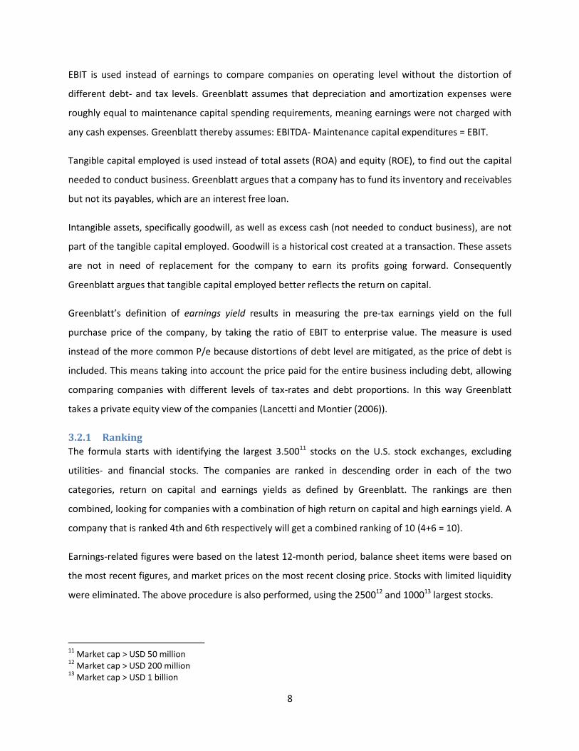
3.2.1 Ranking

The formula starts with identifying the largest 3.50011 stocks on the U.S. stock exchanges, excluding

utilities- and financial stocks. The companies are ranked in descending order in each of the two

categories, return on capital and earnings yields as defined by Greenblatt. The rankings are then

combined, looking for companies with a combination of high return on capital and high earnings yield. A

company that is ranked 4th and 6th respectively will get a combined ranking of 10 (4+6 = 10).

Earnings-related figures were based on the latest 12-month period, balance sheet items were based on

the most recent figures, and market prices on the most recent closing price. Stocks with limited liquidity

were eliminated. The above procedure is also performed, using the 250012 and 100013 largest stocks.

11

Market cap > USD 50 million 12

Market cap > USD 200 million 13

Market cap > USD 1 billion

9

The portfolio consists of, on average, the 30 highest ranked companies at every rebalancing of the

portfolio. Initially, five to seven stocks are picked during the first few months until 30 stocks are reached.

Each time the group of stocks reach one year in the portfolio, rebalancing is done and the highest

ranked stocks replace the previous held stocks.

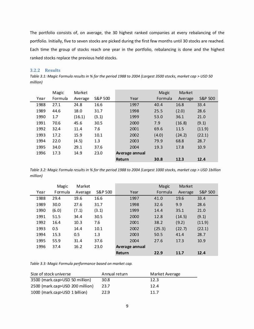
3.2.2 Results Table 3.1: Magic Formula results in % for the period 1988 to 2004 (Largest 3500 stocks, market cap > USD 50

million)

Year

Magic

Formula

Market

Average S&P 500 Year

Magic

Formula

Market

Average S&P 500

1988 27.1 24.8 16.6 1997 40.4 16.8 33.4

1989 44.6 18.0 31.7 1998 25.5 (2.0) 28.6

1990 1.7 (16.1) (3.1) 1999 53.0 36.1 21.0

1991 70.6 45.6 30.5 2000 7.9 (16.8) (9.1)

1992 32.4 11.4 7.6 2001 69.6 11.5 (11.9)

1993 17.2 15.9 10.1 2002 (4.0) (24.2) (22.1)

1994 22.0 (4.5) 1.3 2003 79.9 68.8 28.7

1995 34.0 29.1 37.6 2004 19.3 17.8 10.9

1996 17.3 14.9 23.0

30.8 12.3 12.4

Average annual

Return

Table 3.2: Magic Formula results in % for the period 1988 to 2004 (Largest 1000 stocks, market cap > USD 1billion

million)

Year

Magic

Formula

Market

Average S&P 500 Year

Magic

Formula

Market

Average S&P 500

1988 29.4 19.6 16.6 1997 41.0 19.6 33.4

1989 30.0 27.6 31.7 1998 32.6 9.9 28.6

1990 (6.0) (7.1) (3.1) 1999 14.4 35.1 21.0

1991 51.5 34.4 30.5 2000 12.8 (14.5) (9.1)

1992 16.4 10.3 7.6 2001 38.2 (9.2) (11.9)

1993 0.5 14.4 10.1 2002 (25.3) (22.7) (22.1)

1994 15.3 0.5 1.3 2003 50.5 41.4 28.7

1995 55.9 31.4 37.6 2004 27.6 17.3 10.9

1996 37.4 16.2 23.0

22.9 11.7 12.4

Average annual

Return

Table 3.3: Magic Formula performance based on market cap.

Size of stock universe Annual return Market Average

3500 (mark.cap>USD 50 million) 30.8 12.3

2500 (mark.cap>USD 200 million) 23.7 12.4

1000 (mark.cap>USD 1 billion) 22.9 11.7

10

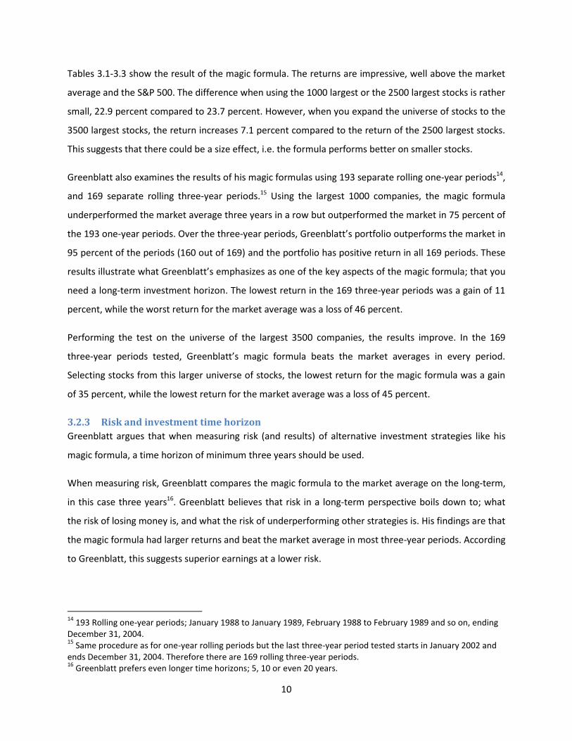
Tables 3.1-3.3 show the result of the magic formula. The returns are impressive, well above the market

average and the S&P 500. The difference when using the 1000 largest or the 2500 largest stocks is rather

small, 22.9 percent compared to 23.7 percent. However, when you expand the universe of stocks to the

3500 largest stocks, the return increases 7.1 percent compared to the return of the 2500 largest stocks.

This suggests that there could be a size effect, i.e. the formula performs better on smaller stocks.

Greenblatt also examines the results of his magic formulas using 193 separate rolling one-year periods14,

and 169 separate rolling three-year periods.15 Using the largest 1000 companies, the magic formula

underperformed the market average three years in a row but outperformed the market in 75 percent of

the 193 one-year periods. Over the three-year periods, Greenblatt’s portfolio outperforms the market in

95 percent of the periods (160 out of 169) and the portfolio has positive return in all 169 periods. These

results illustrate what Greenblatt’s emphasizes as one of the key aspects of the magic formula; that you

need a long-term investment horizon. The lowest return in the 169 three-year periods was a gain of 11

percent, while the worst return for the market average was a loss of 46 percent.

Performing the test on the universe of the largest 3500 companies, the results improve. In the 169

three-year periods tested, Greenblatt’s magic formula beats the market averages in every period.

Selecting stocks from this larger universe of stocks, the lowest return for the magic formula was a gain

of 35 percent, while the lowest return for the market average was a loss of 45 percent.

3.2.3 Risk and investment time horizon

Greenblatt argues that when measuring risk (and results) of alternative investment strategies like his

magic formula, a time horizon of minimum three years should be used.

When measuring risk, Greenblatt compares the magic formula to the market average on the long-term,

in this case three years16. Greenblatt believes that risk in a long-term perspective boils down to; what

the risk of losing money is, and what the risk of underperforming other strategies is. His findings are that

the magic formula had larger returns and beat the market average in most three-year periods. According

to Greenblatt, this suggests superior earnings at a lower risk.

14

193 Rolling one-year periods; January 1988 to January 1989, February 1988 to February 1989 and so on, ending December 31, 2004. 15

Same procedure as for one-year rolling periods but the last three-year period tested starts in January 2002 and ends December 31, 2004. Therefore there are 169 rolling three-year periods. 16

Greenblatt prefers even longer time horizons; 5, 10 or even 20 years.

11

Greenblatt’s view of risk is different from the traditional. He emphasizes the risk of losing money and

use rolling long-term performance as a proxy for that. He does not like the traditional view of volatility

as a measure of risk. This is why we think it is interesting to examine his returns using traditional views

of risk.

The investment time horizon is an issue that Greenblatt’s highlights as important when understanding

how investors make their decisions. Many investment professionals follow the herd of investors

avoiding the risk of poor performance in comparison to peer investors. Professional investors losing

money during an extended time period may be subject to sanctions; losing their job, clients, or capital

needed. This is a potential reason why long-term investment strategies e.g. the magic formula are

disregarded, and also why they perform well (a strategy followed by the entire universe of investors will

obviously not beat the market average).

3.3 Greenblatt versus Efficient market hypothesis The efficient market hypothesis suggests that investors price stocks at a fair value at all times. The EMH

is the main framework used in criticizing trading strategies, among them Greenblatt’s magic formula.

Some of the main critiques brought forward, and dismissed, by Greenblatt are; data mining, look-ahead

bias, survivorship bias, mispricing of risk and size effect.

As for data mining, Greenblatt assures that the two factors in his model were used by him when

investing, prior to the construction of the magic formula. Greenblatt also assures that these were the

two first factors that he back tested.

In his tests, Greenblatt used Compustat, which is a point-in-time database. This means that the database

contains the exact information available to Compustat users on each date in the test, ensuring no look-

ahead bias. Compustat furthermore corrects information that might otherwise produce false positive

results in a back test. It restores companies taken out of the database because of insolvency or a

merger, which avoids the survivorship bias (Alpert).

As mentioned in section 3.2.3, Greenblatt argues that his portfolio is subject to lower risk than the

market average in the long-term horizon, which would mean no mispricing of risk. Furthermore, the

small-size effect does not seem to be the reason for the high returns, since Greenblatt’s formula

12

performs well even for companies with market cap above USD 1 billion, the largest 1000 U.S Stocks.17

3.4 Previous Back Testing of the Greenblatt’s work Back tests of Greenblatt’s results have been done by ClariFI18, finding similar results. The results are an

average return of 28 percent (compared to Greenblatt’s 30.8 percent) using the largest 3500 U.S stocks,

and 17.5 percent (22.9 percent) using the largest 1000 U.S. stocks. These results give credibility to

Greenblatt’s findings since the results are (almost) replicable. Greenblatt’s unrevealed definition of

excess cash could be one of the explanations to why the results differ in the ClariFI back test.

There is no indication that Greenblatt intentionally engaged in data mining. In any case, it is interesting

to see how his strategy performs on a different set of data, i.e. an out-of-sample test. Tests performed,

ranging from finance professor Robert Haugen to Dresdner Kleinwort Wasserstein Securities19 (DRKW),

applying Greenblatt’s strategy to the markets of Europe, Japan and the U.S. The research done by DRKW

finds results showing that Greenblatt’s formula achieves high return in other countries than the U.S.

DRKW compares their results only to the market average, not any alternative strategies. Haugen on the

other hand makes comparisons between different strategies, including his own and Greenblatt’s, on U.S.

stocks.

Before presenting Haugen’s findings, we will present Greenblatt’s comparisons with Haugen’s multi-

factor model. Greenblatt compares his results to Haugen- and Baker’s 71-factor model, on the

Compustat data. The 71-factor model was tested and compared to Greenblatt’s magic formula using

highest and lowest deciles performance20, over the period February 1994 through November 2004, on

the 1000 largest stocks (market cap over $ 1 billion). The two tables show the results when rebalancing

each month and once a year, respectively.

17

Even though it performs even better using smaller stocks as well. 18 Develops and sells financial-modeling software that quantitative investors use to test strategies on data like

Compustat's. 19

DRKW through Montier and Lancetti. 20

Haugen does not suggest investment in the highest decile, nor holding stocks for one year.

13

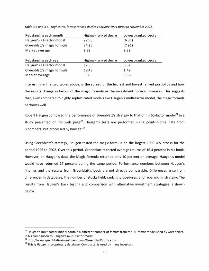
Table 3.5 and 3.6: Highest vs. lowest ranked deciles February 1994 through November 2004.

Rebalancing each month Highest-ranked decile Lowest-ranked decile

Haugen’s 71-factor model 22.98 (6.91)

Greenblatt’s magic formula 24.25 (7.91)

Market average 9.38 9.38

Rebalancing each year Highest-ranked decile Lowest-ranked decile

Haugen’s 71-factor model 12.55 6.92

Greenblatt’s magic formula 18.43 1.49

Market average 9.38 9.38

Interesting in the two tables above, is the spread of the highest and lowest ranked portfolios and how

the results change in favour of the magic formula as the investment horizon increases. This suggests

that, even compared to highly sophisticated models like Haugen’s multi-factor model, the magic formula

performs well.

Robert Haugen compared the performance of Greenblatt’s strategy to that of his 65-factor model21 in a

study presented on his web page22. Haugen’s tests are performed using point-in-time data from

Bloomberg, but processed by himself.23

Using Greenblatt’s strategy, Haugen tested the magic formula on the largest 1000 U.S. stocks for the

period 1996 to 2002. Over this period, Greenblatt reported average returns of 16.4 percent in his book.

However, on Haugen's data, the Magic formula returned only 10 percent on average. Haugen's model

would have returned 17 percent during the same period. Performance numbers between Haugen´s

findings and the results from Greenblatt’s book are not directly comparable. Differences arise from

differences in databases, the number of stocks held, ranking procedures, and rebalancing strategy. The

results from Haugen’s back testing and comparison with alternative investment strategies is shown

below.

21

Haugen’s multi factor model contain a different number of factors from the 71-factor model used by Greenblatt, in his comparison to Haugen’s multi-factor model. 22

http://www.quantitativeinvestment.com/GreenblattStudy.aspx 23

This is Haugen’s proprietary database. Compustat is used by many investors.

14

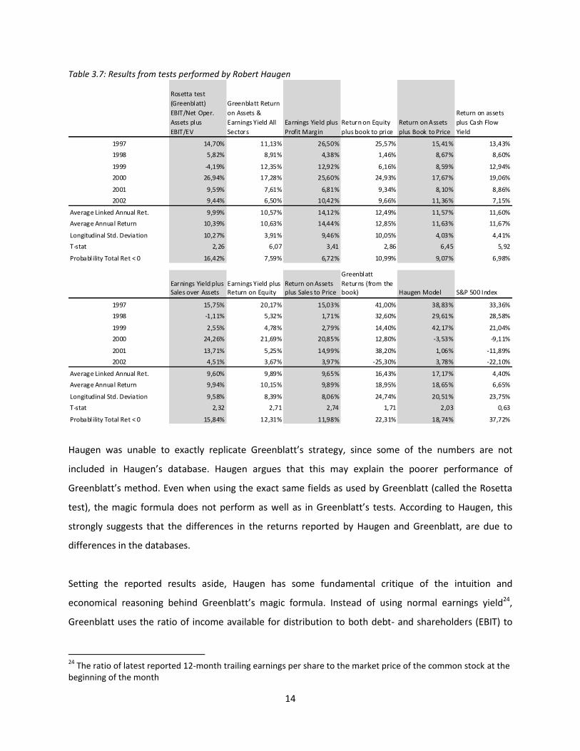
Table 3.7: Results from tests performed by Robert Haugen

Rosetta test

(Greenblatt)

EBIT/Net Oper.

Assets plus

EBIT/EV

Greenblatt Return

on Assets &

Earnings Yield All

Sectors

Earnings Yield plus

Profit Margin

Return on Equity

plus book to price

Return on Assets

plus Book to Price

Return on assets

plus Cash Flow

Yield

1997 14,70% 11,13% 26,50% 25,57% 15,41% 13,43%

1998 5,82% 8,91% 4,38% 1,46% 8,67% 8,60%

1999 -4,19% 12,35% 12,92% 6,16% 8,59% 12,94%

2000 26,94% 17,28% 25,60% 24,93% 17,67% 19,06%

2001 9,59% 7,61% 6,81% 9,34% 8,10% 8,86%

2002 9,44% 6,50% 10,42% 9,66% 11,36% 7,15%

Average Linked Annual Ret. 9,99% 10,57% 14,12% 12,49% 11,57% 11,60%

Average Annual Return 10,39% 10,63% 14,44% 12,85% 11,63% 11,67%

Longitudinal Std. Deviation 10,27% 3,91% 9,46% 10,05% 4,03% 4,41%

T-stat 2,26 6,07 3,41 2,86 6,45 5,92

Probabl ility Total Ret < 0 16,42% 7,59% 6,72% 10,99% 9,07% 6,98%

Earnings Yield plus Sales over Assets

Earnings Yield plus Return on Equity

Return on Assets plus Sales to Price

Greenblatt

Returns (from the book) Haugen Model S&P 500 Index

1997 15,75% 20,17% 15,03% 41,00% 38,83% 33,36%

1998 -1,11% 5,32% 1,71% 32,60% 29,61% 28,58%

1999 2,55% 4,78% 2,79% 14,40% 42,17% 21,04%

2000 24,26% 21,69% 20,85% 12,80% -3,53% -9,11%

2001 13,71% 5,25% 14,99% 38,20% 1,06% -11,89%

2002 4,51% 3,67% 3,97% -25,30% 3,78% -22,10%

Average Linked Annual Ret. 9,60% 9,89% 9,65% 16,43% 17,17% 4,40%

Average Annual Return 9,94% 10,15% 9,89% 18,95% 18,65% 6,65%

Longitudinal Std. Deviation 9,58% 8,39% 8,06% 24,74% 20,51% 23,75%

T-stat 2,32 2,71 2,74 1,71 2,03 0,63

Probabl ility Total Ret < 0 15,84% 12,31% 11,98% 22,31% 18,74% 37,72%

Haugen was unable to exactly replicate Greenblatt’s strategy, since some of the numbers are not

included in Haugen’s database. Haugen argues that this may explain the poorer performance of

Greenblatt’s method. Even when using the exact same fields as used by Greenblatt (called the Rosetta

test), the magic formula does not perform as well as in Greenblatt’s tests. According to Haugen, this

strongly suggests that the differences in the returns reported by Haugen and Greenblatt, are due to

differences in the databases.

Setting the reported results aside, Haugen has some fundamental critique of the intuition and

economical reasoning behind Greenblatt’s magic formula. Instead of using normal earnings yield24,

Greenblatt uses the ratio of income available for distribution to both debt- and shareholders (EBIT) to

24

The ratio of latest reported 12-month trailing earnings per share to the market price of the common stock at the beginning of the month

15

the market value of equity plus the face value of debt. Haugen argues that this measure the

“cheapness” of a combined investment in the firm's debt and equity. Haugen claims that this do not

make sense when only investing in equity, as Greenblatt’s strategy suggests.

Haugen argues that Greenblatt's version of earnings yield can actually be seen as a blend of two ratios.

He decomposes it as follows; E is income available for distribution to stockholders, I is interest paid on

debt, P is the market value of the stock, and D is the face value of the debt. Greenblatt's version of

earnings yield is therefore (E+I)/(P+D). The ratio is E/P, is generally known as earnings yield and well

known in the investment community. The ratio, I/D, is the ratio of interest expense to face value of debt.

Haugen further explains that the size of this ratio is determined by: the credit worthiness of the

company, the term of the debt, and the interest rates when issuing debt. Haugen argues that the ratio

employed by Greenblatt as an earnings yield version has no explanatory effect or economic sense.

Furthermore, the results are not better than when using the classical earnings yield, or any other version

of this measurement, according to tests presented above.

3.5 The possibility to use anomalies as trading strategies The predictive power of the anomalies on stock returns are of interest when evaluating Greenblatt’s

trading strategy. We will in this section assess the possibility to use the anomalies when designing

investment strategies.

The anomalies presented represent a significant amount of evidence against the EMH. There are

however strong arguments made that these anomalies have common problems, suggesting that the

market is efficient. We will present some of these problems below.

Firstly, one problem argued by e.g. Schwert (2003) is data mining. Researchers use data samples to find

anomalies that contradict the EMH. Schwert argues that researchers perform their tests trying to mount

evidence against the current accepted knowledge, in this case the EMH. This would suggest that the

anomalies cannot be used as a trading strategy, as it is a pure statistical construction.

Secondly, a problem common to the anomalies is that even if they are statistically significant during

some research periods they show now economic significance, i.e. you cannot take advantage of those

anomalies to earn abnormal profits (Malkiel (2003)).

16

Thirdly, another important critique of the anomalies is that they fail to be consistent over time. One

example is the shifting performance of the momentum strategy, which leads to abnormal positive

returns during the late 1990s but highly negative returns during 2000 (Malkiel (2003)).

Fourthly, another problem facing some of the anomalies is the self-destructing effect the finding and

publishing of the anomalies have. The possibility to use the anomaly as a trading strategy may disappear

because investors are handed a free lunch and make use of it until no profits can be made with that

particular trading strategy.

3.6 The anomalies and Greenblatt It is interesting to see the connection between Greenblatt’s formula and the anomalies presented. For

example, a high earnings yield25, which Greenblatt uses, is closely associated with low P/e. Both

measures premiere companies that has low ratio between earnings and price. Basu (1977) found that

stocks with low P/e outperformed, which could be an indicator that a high earnings yield is a good

measure to identify winners.

The contrarian strategy is also interesting when it comes to Greenblatt’s measures, since it is possible

that companies that have a high earnings yield due to a low price, has been a loser over the last couple

of years. Hence, the earnings yield could possibly identify contrarian stocks.

Greenblatt’s findings have a connection to the size effect, since his formula performs substantially

better when using a market cap of USD 50 million as cut-off point for which stocks to include compared

to using USD 200 million or USD 1 billion.

4 Method and Data

4.1 Method We will try to imitate Greenblatt’s procedures to as a large extent as possible. However, some

comments on our procedures are necessary.

We will perform rankings every month for the period starting January 1998 and ending December 2007.

The start date of the accumulation of the stocks to our portfolio is January 1st 1998 and the final date of

25

Greenblatt uses EBIT/EV as earnings yield. It is common to use earnings/profit as earnings yield.

17

the portfolio will be January 1st 2008. The stock market is typically not open on those dates, but there

are values for those dates in the Datastream database and it is those values that we will use26. The same

procedure will be used for other dates when the stock market is closed.

The data from the companies is sorted into different periods. One period represents a month, so in total

we will have 120 periods. We perform the rankings on the first day in each month and the stocks will be

added to the portfolio the same day.

Exactly what items Greenblatt uses in his rankings is somewhat unclear. We will therefore create two

portfolios that we will test. The portfolio that we believe to be most in line with Greenblatt’s will use

EBIT/ (Net Working Capital + Net Fixed Assets27) as return on capital. This portfolio will be called

Portfolio I. The other portfolio will use EBIT / Capital Employed28 as return on capital. This portfolio will

be called Portfolio II. We believe that the latter portfolio could be a better indicator of the performance

of the company since it also includes intangible assets such as goodwill, patents and licences etcetera.

We argue that these assets should be included because companies use these asset types to get their

earnings and should therefore be a part of the measure. Otherwise it could create a bias towards

companies that have little fixed assets and large intangible assets. Both portfolios will use EBIT/EV as

earnings yield.

We will accumulate the stocks gradually during the first year by adding the two stocks that rank the

highest in each month. Hence, it will take until the twelfth ranking until the portfolio is full. The full

portfolio consists of 24 stocks. The two stocks selected by the rankings will be a part of the portfolio for

twelve months. After that the two stocks will be sold off and two new stocks selected by the rankings

will be added to the portfolio. Stocks that are being sold off in a period can, if selected by the rankings,

be picked up in the same period and will then be held for another twelve month period. If the rankings

select a stock that already is a part of the portfolio, the next stock that is not part of the portfolio will be

added.

26

Datastream uses the previous day’s closing price in those cases. 27

We uses Datastream’s “Total Fixed Assets – Net” as Net Fixed Assets. 28

As defined in the Datastream data base.

18

Figure 4.1: Holding of the stocks

Month 0 1 2 3 4 5 6 7 8 9 10 11 12 13 14 15 …

1st pair

2nd pair

3rd Pair

4th pair

Etc

We will in the study also see what happens if we add transaction costs. The transaction costs will be

calculated as a monthly percentage of the portfolio value. We arrived to the monthly percentage of 0.2

percent (20 basis points). The reasoning behind that number is as follow. The commission on each trade

is assumed to be 15 basis points per transaction29. In each month the portfolio sells two stocks and buy

stocks; that is four transactions. 15 basis points times four equals 60 basis points. However, the

transactions each month only represent 1/12 of portfolio value, which brings us down to five (60/12)

basis points of portfolio value. But we wanted a larger number than that to reflect potential market

impact and possible rebalancing that has to be made to keep the portfolio equally weighted. And that is

why we use 0.2 percent. This is not an exact measure of the transaction cost, but it gives a more realistic

picture of the performance than without using transaction costs.

One problem with the kind of rankings that we perform is the problem of look-ahead bias. Look-ahead

bias is that you at a historic point in time use information that was not available for the people who lived

then. For example, if you use company X’s EBIT for the full year 2006 at January 1st 2007, you are subject

to look-ahead bias since company X’s annual accounts for 2006 is typically not available at January 1st

2007. The database that we have used, Datastream, does not take this into account. In order to reduce

the effects of look-ahead bias, we use a two month lag, e.g. the numbers for 2006 for a company that

uses a normal calendar year will not be in the rankings until March 1st 2007. We use a two-month lag

since most companies tend to report their full year earnings in the end of January or early February. We

did not want to use just a one-month lag, since there are companies that have not report by then and it

is better for the reliability of our model to have a disadvantage compared to an advantage. We realize

29

This number tend to be what the major brokerage firms in the Nordic region charge their institutional clients.

19

that this is not a perfect solution, since some companies report within a month after their financial year

expires and some does not report within two months after expiration of the financial years, but we

believe this is a good approximation that makes the rankings more in line what the rankings would have

looked.

The monthly return of the portfolios will be tested against the CAPM and Fama-French’s three factor

model. CAPM is (Cochrane(1999)):

(i) )( ftmtitftit rrrr

or as testable in a regression:

(ii) )( ftmtitiftit rrrr

where

itr = return of asset I at time t,

ftr = return of the risk free rate at time t,

mtr = return of the market portfolio at time t.

When testing against CAPM, we decided to use two different proxies for the market portfolio. Since we

did the study on a Nordic basic, we used the benchmark MSCI Nordic as one proxy30. However, since the

argument can be made that the Nordic region is not diversified enough to represent the market

portfolio, we also used the market portfolio from database on Kenneth French’s homepage31. As seen

later, which proxy we use does not affect the results.

The Fama-French’s three factor model is (Fama (1998)):

(iii) )()()( tittitftmtitftit HMLhSMBsrrrr

or

(iv) )()()( tittitftmtitiftit HMLhSMBsrrrr

30

With 12 month Stockholm Interbank Offered Rate (STIBOR) as the risk free rate. 31

http://mba.tuck.dartmouth.edu/pages/faculty/ken.french/data_library.html

20

where

itr = return of asset I at time t,

ftr = return of the risk free rate at time t,

mtr = return of the market portfolio at time t,

SMBt = return of the Small minus Big portfolio at time t,

HMLt = return of the High minus Low portfolio at time t.

We will also calculate the Sharpe ratio for the portfolios and benchmark. The Sharpe ratio is (Sharpe

(1994)):

(v) i

fi

i

rrS

where

ir = the mean return of asset I,

fr = the mean return of the risk free rate,

i = the standard deviation of asset i.

4.2 Bad model problem and the Joint Hypothesis Problem In order for a strategy to violate EMH it is not sufficient for the strategy to just have higher returns than

the market. Remember, a strategy that leads to large returns can be explained by that the strategy takes

on a large amount of risk. The strategy has to earn abnormal return, i.e. the return has to be above what

the risk specifies. In order to test for this, you need to have an asset-pricing model that specifies what

return you should earn given the risk. An observant reader will here discover a problem. The test that

you will perform will be dependent on the asset-pricing model that you use. It becomes a joint

hypothesis problem since you will test both the asset-pricing model and EMH (in form of if the return is

abnormal). If the asset-pricing model is miss-specified, the test may lead to the wrong conclusion since

21

the test can fail for two reasons. Either because one of the two hypotheses is false or because both parts

of the joint hypothesis are false. And you cannot determine which one it is. (Fama (1991), Jensen (1978))

4.3 Data The stocks included in our study are all the stocks listed on five stock exchanges in the Nordic region:

Copenhagen, Helsinki, Oslo, Reykjavik and Stockholm. We use data from the Datastream database

between 1996 and 2008. Most of the data is the form of company account data on annual basis.

However, prices on the stocks are on a monthly basis. The prices of the MSCI Nordic and S&P 500 index

are also from Datastream. For the Nordic risk free rate we used 12 month STIBOR from the Swedish

Riksbank’s homepage. The three Fama-French factors – Market return minus risk free rate, High-Minus-

Low and Small-Minus-Big - are downloaded from Kenneth French’s beautiful homepage32.

The original number of stocks was 1184. Just as Greenblatt did, we excluded the stocks of financial33 and

utility companies. We also made sure that there only was one type of share representing each company.

Unfortunately, for some companies there was not sufficient data in the database and we therefore had

to exclude them. It is obviously a problem that companies that should have been a part of the sample

had to be excluded. However, since it is most likely completely random which companies did not have

sufficient data, this is not likely to interfere with our results. After these procedures, 744 stocks are

remaining for our study34.

5 Hypothesis Is Greenblatt’s finding for real or is it just pure luck? Since the two measures that he used was the first

that he tested for, the case of data mining is not applicable, but it could be luck. In a large set of historic

stock data, a large number of patterns will appear. And stocks that produce above market returns will

share some common patterns. But unless the factors that constitute the patterns are things that cause

the above market returns, then the patterns are of no use. For example, Jason Zwieg (1999) from Money

Magazine found by using 10 500 stocks between 1980 and 1999, you could have beaten the market with

1.3 percents by just buying stocks that have no repeat letters in its name. By all this we are trying to say

that just because Greenblatt managed to get above market return in his sample, it is not certain that we

will receive the same when using the formula in the Nordics.

32

http://mba.tuck.dartmouth.edu/pages/faculty/ken.french/data_library.html 33

Banks, asset managers, clearing houses, brokerage firms and insurance companies. 34

For a complete list of the companies in the study, see appendix.

22

However, there is an economic intuition behind Greenblatt’s formula that is reasonable (buy companies

that create good return on their assets cheap), although Haugen disagrees. Furthermore, the study

performed by Dresdner Kleinwort showed that the magic formula outperformed in other regions as

well.

With all this in mind we get our first hypothesis, which is that the absolute return of the tested

portfolios will be above the return of the market.

Hypothesis 1a. Portfolio I achieves higher return than the Fama-French’s market portfolio and broad

market indices. The market indices that we use are S&P 500 Composite and MSCI Nordic.

Hypothesis 1b. Portfolio II achieves higher return than the Fama-French’s market portfolio and broad

market indices.

As we mentioned in section 4.1, we believe that by using Capital Employed instead of Net Working

Capital + Net Fixed Assets we better reflect the state of the companies. We therefore believe that this

strategy will achieve a higher return than Greenblatt’s original formula. This will be our second

hypothesis.

Hypothesis 2. Our strategy achieves higher return than Greenblatt’s, i.e. Portfolio II will achieve a higher

return than Portfolio I.

According to Finance theory a high return could be explained by high risk. Greenblatt does not talk

extensively about risk and he does not risk adjust the return of his portfolios. If Greenblatt’s formula

produce abnormal returns, then his findings are really interesting. By this we arrive to our third

hypothesis, which is if the Magic formula does not outperform the market when risk adjusted.

As discussed before about bad model we cannot have the EMH as a hypothesis. We therefore have to

break down EMH to testable hypothesis. We decided to use arguably the two most famous and used

asset pricing models; Capital Asset Pricing Model (CAPM) and Fama-French’s three-factor model.

Hypothesis 3a. Portfolio I’s return is explained by CAPM, i.e. the alpha is not significant.

Hypothesis 3b. Portfolio II’s return is explained by CAPM, i.e. the alpha is not significant.

Hypothesis 4a. Portfolio I’s return is explained by Fama-French’s three factor model, i.e. the alpha is not

significant.

Hypothesis 4b. Portfolio II’s return is explained by Fama-French’s three factor model, i.e. the alpha is

not significant.

23

6 Results

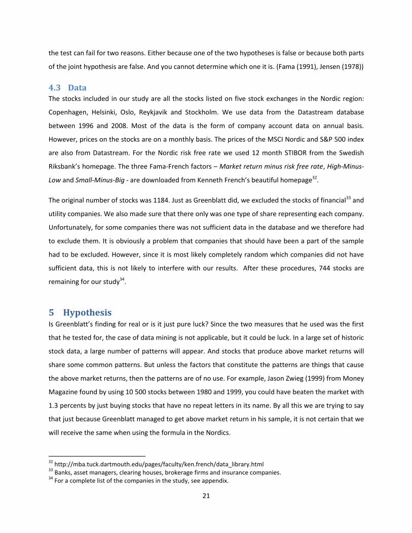
6.1 Hypothesis 1 Table 6.1: Monthly descriptives (except CAGR which is on an annual basis) of the market portfolio, S&P 500

Composite, MSCI Nordic, Portfolio I and Portfolio II for the whole sample period.

Portfolio I Portfolio II Mkt

Mean 0,0132 Mean 0,0233 Mean 0,0065

Median 0,0080 Median 0,0168 Median 0,0123

Standard Deviation 0,0592 Standard Deviation 0,1040 Standard Deviation 0,0447

Minimum -0,1750 Minimum -0,1482 Minimum -0,1577

Maximum 0,1555 Maximum 1,0114 Maximum 0,0839

CAGR 0,1468 CAGR 0,2609 CAGR 0,0677

Sharpe 0,1739 Sharpe 0,1957 Sharpe 0,0800

S&P 500 Composite MSCI Nordic

Mean 0,0043 Mean 0,0102

Median 0,0056 Median 0,0104

Standard Deviation 0,0414 Standard Deviation 0,0744

Minimum -0,1062 Minimum -0,1794

Maximum 0,1269 Maximum 0,2389

CAGR 0,0423 CAGR 0,0928

Sharpe 0,0338 Sharpe 0,0973

Both Portfolio I and Portfolio II achieve a higher return than the Market portfolio, S&P 500 and MSCI

Nordic, which is what we expected. Both our portfolios achieve impressive compounded annual growth

rates (CAGR), 14.68 percent for Portfolio I and 26.09 percent for Portfolio II. The standard deviation of

the Market portfolio and S&P 500 is lower than our portfolios, which is also expected. However, the

standard deviation of MSCI Nordic is higher than the standard deviations of Portfolio I; but Portfolio II

has a higher standard deviation. The Sharpe ratio is higher for both Portfolio I and Portfolio II compared

to the benchmarks.

24

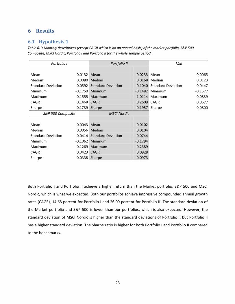
Figure 6.1: The aggregated returns of Portfolio I, Portfolio II, Market portfolio (Mkt), S&P 500 Composite and MSCI

Nordic. (Start value for all portfolios is 100)

In figure 6.1 we can see the aggregated returns of the different portfolios and indices. As seen, Portfolio

II is a clear-cut winner with Portfolio I as a clear runner-up. If you had invested SEK 100 in Portfolio at

the start of 1998, you would have SEK 1015 at January 1st 2008, which represents a return of 915

percent. A SEK 100 investment in Portfolio I in 1998 would have led to SEK 393 at the end of the period.

We can conclude that Portfolio I and Portfolio II achieve higher return (and a higher Sharpe ratio) than

the market portfolio and the market indices that we used. We therefore accept hypothesis 1a and 1b.

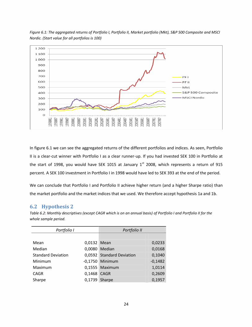
6.2 Hypothesis 2 Table 6.2: Monthly descriptives (except CAGR which is on an annual basis) of Portfolio I and Portfolio II for the

whole sample period.

Portfolio I Portfolio II

Mean 0,0132 Mean 0,0233





CAGR 0,1468 CAGR 0,2609


25

As seen in table 6.2 the both portfolios have a positive mean, Portfolio I 1.32 percent and Portfolio II

2.33 percent. Portfolio II also has a higher median than Portfolio I. An explanation for that Portfolio II

has a higher return is that it takes on more risk; Portfolio II has a standard deviation of 10.4 percent

compared to 5.92 percent for Portfolio I. However, Portfolio I has the lowest minimum value indicating

that Portfolio I has the lowest single month drop in the portfolio value. Portfolio II also has a higher

Sharpe ratio than Portfolio I

We can therefore conclude that Portfolio II achieves a higher return than Portfolio I. We therefore

accept hypothesis 2.

6.3 Hypothesis 3 We now move on to the hypothesis regarding EMH, which is the heart and soul of this thesis.

Table 6.3: Regression table using the return of Portfolio I as dependable variable and Mkt-RF as explanatory

variable.

Coefficients Standard Error t Stat P-value

Intercept 0,0078 0,0046 1,6817 0,0953

Mkt-RF 0,7024 0,1034 6,7950 0,0000000

Table 6.4: Regression table using the return of Portfolio I as dependable variable and MSCI – 12 month STIBOR as

explanatory variable.

Coefficients Standard

Error t Stat P-value

Intercept 0,0070 0,0045 1,5432 0,1254

MSCI Nordic - 12M 0,4521 0,0604 7,4794 1,45E-11

The intercept (alpha) is positive when using Mkt-RF as explanatory variable. However, the P-value is

quite high. The coefficient for Mkt-RF is positive and significant on all reasonable significant levels. The

same analysis can be made when MSCI – 12M is the explanatory variable. Hence, we cannot reject

hypothesis 3a that the return of Portfolio I is explained by CAPM.

26

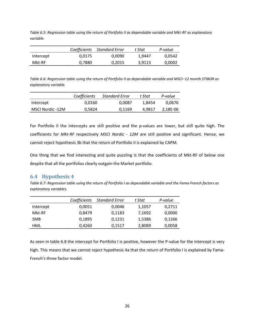
Table 6.5: Regression table using the return of Portfolio II as dependable variable and Mkt-RF as explanatory

variable.


Intercept 0,0175 0,0090 1,9447 0,0542

Mkt-RF 0,7880 0,2015 3,9113 0,0002

Table 6.6: Regression table using the return of Portfolio II as dependable variable and MSCI–12 month STIBOR as

explanatory variable.


Intercept 0,0160 0,0087 1,8454 0,0676

MSCI Nordic -12M 0,5824 0,1169 4,9817 2,18E-06

For Portfolio II the intercepts are still positive and the p-values are lower, but still quite high. The

coefficients for Mkt-RF respectively MSCI Nordic - 12M are still positive and significant. Hence, we

cannot reject hypothesis 3b that the return of Portfolio II is explained by CAPM.

One thing that we find interesting and quite puzzling is that the coefficients of Mkt-RF of below one

despite that all the portfolios clearly outgain the Market portfolio.

6.4 Hypothesis 4 Table 6.7: Regression table using the return of Portfolio I as dependable variable and the Fama-French factors as

explanatory variables.


Intercept 0,0051 0,0046 1,1057 0,2711

Mkt-RF 0,8479 0,1183 7,1692 0,0000

SMB 0,1895 0,1231 1,5386 0,1266

HML 0,4260 0,1517 2,8089 0,0058

As seen in table 6.8 the intercept for Portfolio I is positive, however the P-value for the intercept is very

high. This means that we cannot reject hypothesis 4a that the return of Portfolio I is explained by Fama-

French’s three factor model.

27

Table 6.8: Regression table using the return of Portfolio II as dependable variable and the Fama-French factors as



Intercept 0,0135 0,0091 1,4788 0,1419

Mkt-RF 0,9546 0,2333 4,0906 0,0001

SMB 0,4235 0,2430 1,7432 0,0839

HML 0,6008 0,2992 2,0078 0,0470

We can see in table 6.9 that the intercept for Portfolio II is positive, but once again the P-value for the

intercept is high. We can therefore not reject hypothesis 4b that the return of Portfolio II is explained by

Fama-French’s three factor model.

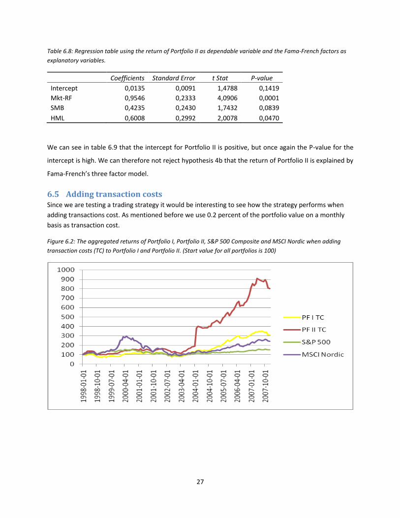
6.5 Adding transaction costs Since we are testing a trading strategy it would be interesting to see how the strategy performs when

adding transactions cost. As mentioned before we use 0.2 percent of the portfolio value on a monthly

basis as transaction cost.

Figure 6.2: The aggregated returns of Portfolio I, Portfolio II, S&P 500 Composite and MSCI Nordic when adding

transaction costs (TC) to Portfolio I and Portfolio II. (Start value for all portfolios is 100)

28

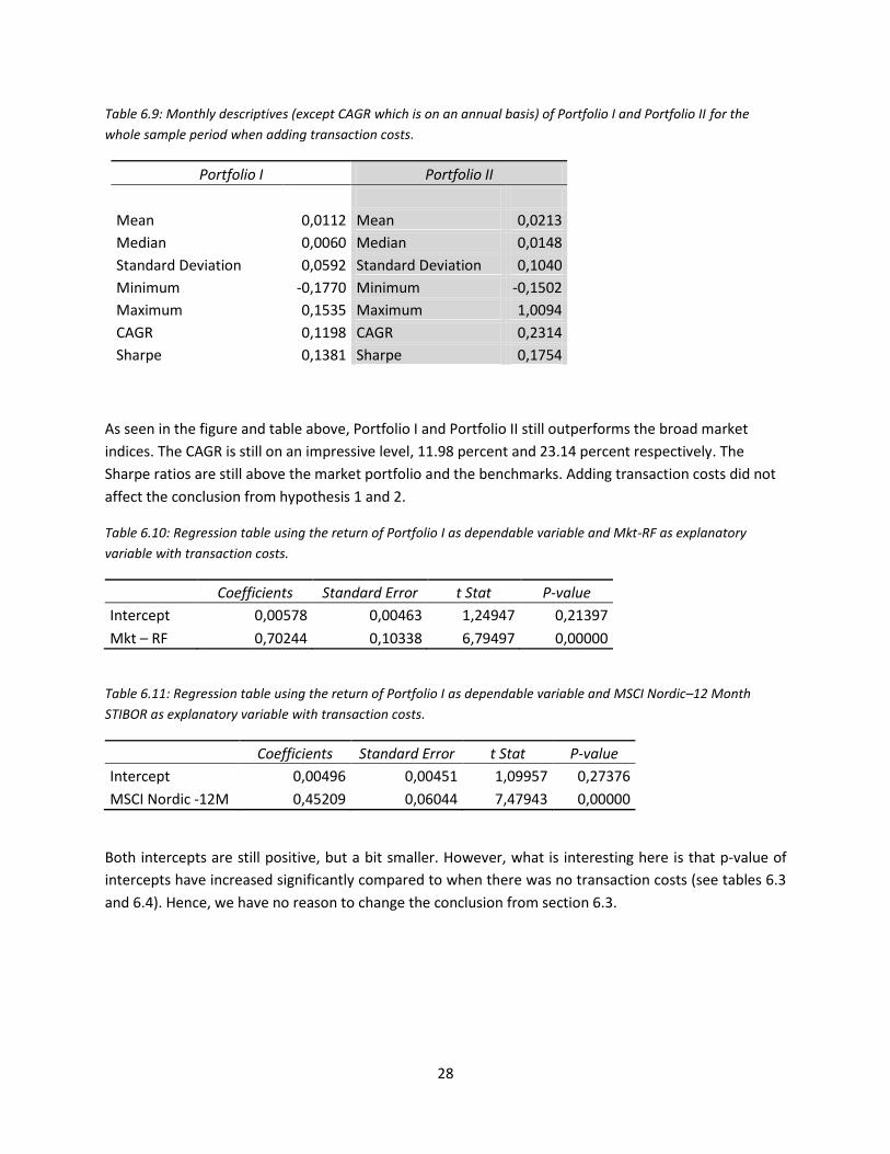
Table 6.9: Monthly descriptives (except CAGR which is on an annual basis) of Portfolio I and Portfolio II for the

whole sample period when adding transaction costs.

Portfolio I Portfolio II

Mean 0,0112 Mean 0,0213





CAGR 0,1198 CAGR 0,2314


As seen in the figure and table above, Portfolio I and Portfolio II still outperforms the broad market

indices. The CAGR is still on an impressive level, 11.98 percent and 23.14 percent respectively. The

Sharpe ratios are still above the market portfolio and the benchmarks. Adding transaction costs did not

affect the conclusion from hypothesis 1 and 2.

Table 6.10: Regression table using the return of Portfolio I as dependable variable and Mkt-RF as explanatory

variable with transaction costs.


Intercept 0,00578 0,00463 1,24947 0,21397

Mkt – RF 0,70244 0,10338 6,79497 0,00000

Table 6.11: Regression table using the return of Portfolio I as dependable variable and MSCI Nordic–12 Month

STIBOR as explanatory variable with transaction costs.


Intercept 0,00496 0,00451 1,09957 0,27376

MSCI Nordic -12M 0,45209 0,06044 7,47943 0,00000

Both intercepts are still positive, but a bit smaller. However, what is interesting here is that p-value of

intercepts have increased significantly compared to when there was no transaction costs (see tables 6.3

and 6.4). Hence, we have no reason to change the conclusion from section 6.3.

29

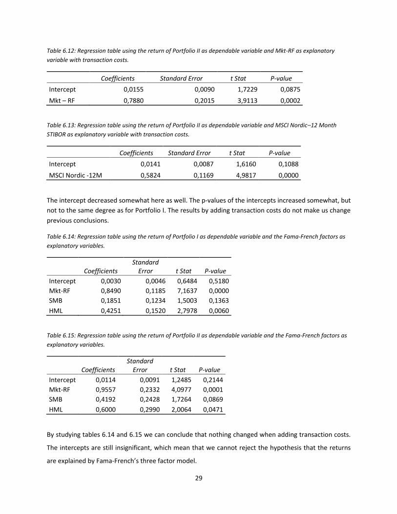
Table 6.12: Regression table using the return of Portfolio II as dependable variable and Mkt-RF as explanatory

variable with transaction costs.


Intercept 0,0155 0,0090 1,7229 0,0875

Mkt – RF 0,7880 0,2015 3,9113 0,0002

Table 6.13: Regression table using the return of Portfolio II as dependable variable and MSCI Nordic–12 Month

STIBOR as explanatory variable with transaction costs.


Intercept 0,0141 0,0087 1,6160 0,1088

MSCI Nordic -12M 0,5824 0,1169 4,9817 0,0000

The intercept decreased somewhat here as well. The p-values of the intercepts increased somewhat, but

not to the same degree as for Portfolio I. The results by adding transaction costs do not make us change

previous conclusions.

Table 6.14: Regression table using the return of Portfolio I as dependable variable and the Fama-French factors as




Intercept 0,0030 0,0046 0,6484 0,5180

Mkt-RF 0,8490 0,1185 7,1637 0,0000

SMB 0,1851 0,1234 1,5003 0,1363

HML 0,4251 0,1520 2,7978 0,0060

Table 6.15: Regression table using the return of Portfolio II as dependable variable and the Fama-French factors as




Intercept 0,0114 0,0091 1,2485 0,2144

Mkt-RF 0,9557 0,2332 4,0977 0,0001

SMB 0,4192 0,2428 1,7264 0,0869

HML 0,6000 0,2990 2,0064 0,0471

By studying tables 6.14 and 6.15 we can conclude that nothing changed when adding transaction costs.

The intercepts are still insignificant, which mean that we cannot reject the hypothesis that the returns

are explained by Fama-French’s three factor model.

30

6.6 Rolling 12 Month Performances The average rolling 12-month return is 21.5 percent for Portfolio I and 36.0 percent for Portfolio II.

However, there is a risk of losing money since both portfolios had quite many negative rolling 12-month

periods. Portfolio I lost money in 25 of the 109 periods (22.9 percent), while Portfolio II lost money in 22

periods (20.2 percent). The probability of losing money could therefore been seen as quite high in our

case. See appendix for complete list of the rolling 12-month performance.

7 Discussions and Conclusions As we have pointed earlier in this thesis, you can with a large set of data by pure luck find patterns

among stocks that perform better than the market. Was this the case with Joel Greenblatt? Probably

not, since others and we managed to get healthy returns above the market by back testing his strategy.

The implications of our results are dependent on how you look at risk and what you believe risk to be.

Our two portfolios had an absolute return above the market. It did however lose money in more than 20

percent of the rolling 12-month periods, which suggest that there is a rather big chance of losing money.

When we risk adjust our portfolios with CAPM and Fama-French’s three factor model, they do not beat

the market. From an EMH perspective this suggests that there is something more risky with this

strategy. That earnings yield could be a proxy for risk is not hard to see, the price of the stock could be

low due to financial distress. That a high return on capital could be a proxy for risk is harder, but not

impossible, to see. It could be that the market expects the company to continue achieving high returns

and therefore pushes up the price. And if the expectations are not met, that would lead to volatility.

However, that combining the two should be a proxy for risk is intuitively hard to understand.

We found that using transaction cost lowered the return (no surprise there) but the intercepts in our

regressions remained insignificant. We also found that using a measure that includes intangible assets

was a better measure to use. That is not surprising to us since we believe such measure better reflect

the state of the company.

Greenblatt stresses, in line with other value investors, that the traditional risk measures have flaws and

are not adequate in the interpretation of risk for an investing strategy. Bearing in mind the development

of risk measures since the CAPM was introduced, we see the point with this criticism. However, we want

to stress the fact that neither Greenblatt, nor any other value investors that we have come across, have

any compelling alternative measure that are quantifiable. This leads us to another interesting question,

31

does it make sense to use statistical measures such as the significances of the intercepts to judge

whether or not an investment strategy is good or bad? We raise this question since it is hard to get

significance intercepts with a limited number of time periods, which often is the case when evaluating

trading strategies. Maybe the best measure of an investment strategy’s performance is the track-record

of an investor putting his money where his mouth is.

The high returns of the magic formula are definitely intriguing. However, we would be caution to use

this strictly as a trading strategy, since the results are not definitive. We are not convinced that the

strategy will achieve high returns going forward. We do believe that the formula could be valuable as a

part of a screening process for which stocks to invest in, since it has in the past shown an ability to pick

good stocks.

8 Further research We think that the most interesting thing to further research is to use the strategy over a longer period,

say 20 or 30 years. That would give a better picture of the risk of the strategy.

It would be interesting to further examine if the formula performs better if updating the corporate

accounts data quarterly and use rolling four quarters. To use more recent data would most likely lead to

a better performance. In our thesis we have used last year’s EBIT when performing the rankings. A

better way to identify future winners could be to use average EBIT for the last couple of years, since this

would better reflect a typical year for the companies. Other things one can try are changing the holding

period and the number of stocks that you buy to see if this affects the performance.

Another interesting thing to examine is to see how the formula performed during the fall of 2008 when

the market dropped significantly. Since our result indicates that the strategy increases the risk it is not

unreasonable to believe that this would come in effect during an event like that. However, by buying

stocks that are cheap, the fall height would probably not be as high. It would also be interesting to see if

the formula could pick future winners by identifying cases where the stock market has overreacted,

which De Bondt and Thaler (1985) showed that it sometimes does.

32

9 Reference list

9.1 Academic references Banz, Rolf W., 1981; The relationship between return and market value of common stocks, Journal of

Financial Economics 9, 3-18.

Basu, Sanjoy, 1977; Investment performance of common stocks in relation to their price earnings ratios:

A test of market efficiency, Journal of Finance 32, 663-682.

Branch, Ben, 1977; A tax loss trading rule, Journal of Business 50, 198–207.

Campbell, John Y. and Robert J. Shiller, 1998; Valuation ratios and the long-run stock market outlook,

Journal of Portfolio Management, 24, 11−26.

Chan, K. C., 1988; On the contrarian investment strategy, Journal of Business 61, 147-163.

Chan, K. C. and Nai-fu Chen, 1991; Structural and return characteristics of small and large firms, Journal

of Finance 46, 1467-1484.

Cochrane, John H, 1999;New Facts In Finance, Economic Perspectives Federal Reserve Bank of Chicago

23(3), pp. 36-58.

Chan, K. C., Yasushi Hamao, and Josef Lakonishok, 1991; Fundamentals and stock returns in Japan,

Journal of Finance 46, 1739-1764.

Cross, Frank, 1973; The Behavior of Stock Prices on Fridays and Mondays, Financial Analysts Journal

29:6, 67-69.

DeBondt, Werner F. M. and Richard H. Thaler, 1985; Does the stock market overreact, Journal of Finance

40, 793-805.

Dyl, Edward A. and Edwin D. Maberly, 1988; A Possible Explanation of the Weekend, Financial Analysts

Journal 44:3, 83-84.

Fama, Eugene, 1970; Efficient Capital Markets: A Review of Theory and Empirical Work, Journal of

Finance 25, 383–417.

Fama, Eugene F. and Kenneth R. French, 1992; The cross-section of expected stock returns, Journal of

Finance 47, 427-66.

Fama, Eugene and Kenneth R. French, 1993; Common Risk Factors in the Returns on Stocks and Bonds, Journal of Finance, 33:1, 3–56.

Fama, E.F. and Kenneth R. French, 1998; Value versus growth: the international evidence, Journal of

Finance 53, 1975−1999.

33

Fama, Eugene F, 1998; Market efficiency, long term returns, and behavioural finance, Journal of

Economics 49, 283-306.

Fama, Eugene and Kenneth R. French, 2001; Disappearing Dividends: Changing Firm Characteristics or

Lower Propensity to Pay, Journal of Financial Economics 60:1, 3– 43.

Fluck , Zsuzsanna, Burton Malkiel and Richard E. Quandt, 1997; The Predictability of Stock Returns:

A Cross-Sectional Simulation, Review of Economics and Statistics 79:2, 176-183.

French, Kenneth R., 1980; Stock returns and the weekend effect, Journal of Financial Economics 8, 55-

70.

Horowitz, Joel L., Tim Loughran and N. E. Savin, 2000; The Disappearing Size Effect, Research in

Economics 54, 83-100.

Jegadeesh, Narasimhan and Sheridan Titman, 1993; Returns to buying winners and selling losers:

implications for stock market efficiency, Journal of Finance 48, 65−91.

Jensen, Michael C., 1978; Some Anomalous Evidence Regarding Market Efficiency, Journal of

Financial Economics 6, 95-101.

Keim, Donald B., 1983; Size-Related Anomalies and Stock Return Seasonality: Further Empirical

Evidence, Journal of Financial Economics 12, 13-32.

Keim, Donald B. and Robert F. Stambaugh, 1984; A Further Investigation of the Weekend Effect in Stock

Returns, Journal of Finance 39:3, 819-835.

Lakonishok, Josef, Anrei Shleifer and Robert W. Vishny, 1994; Contrarian investment, extrapolation, and

risk, Journal of Finance 49, 1541−1578.

Lakonishok, Josef and Seymour Smidt, 1984; Volume and Turn of the year behavior, Journal of Financial

Economics, 435-455.

Lo, Andrew W. and A. Craig MacKinlay, 1988; Stock market prices do not follow random walks: Evidence

from a simple specification test, Review of Financial Studies 1, 41-66.

Malkiel, Burton, 2003; The Efficient Market Hypothesis and Its Critics, Journal of Economic

Perspectives 17:1, 59-82.

Rogalski, Richard J., 1984; New findings Regarding Day-of-the-Week Returns over Trading and Non-

Trading Periods: A Note, Journal of finance 39:5, 1603-1614.

Roll, Richard, 1983; Vas ist das? The turn-of-the-year effect and the return premia of small firms, Journal

of Portfolio Management 9, 18-28.

34

Rubinstein, Mark, 2001; Rational Markets: Yes or No? The Affirmative Case, Financial Analysts Journal

57:3, 15-29.

Schiller, Robert J., 2003; From Efficient Markets Theory to Behavioral Finance, Journal of Economic

Perspectives 17:1, 83-104.

Schwert, G. William, 2003; Anomalies and Market Efficiency, Handbook of the Economics of Finance,

Edited by George Constantinides, Milton Harris, and Rene M. Stulz, North-Holland, 937-972.

Sharpe, W. F. 1994; The Sharpe Ratio, Journal of Portfolio Management 21 (1): 49–58.

Sullivan, Ryan, Allan Timmermann and Halbert White, 2001; Dangers of Data Mining: The Case of

Calendar Effects in Stock Returns, Journal of Econometrics 105, 249-286.

Szyszka, Adam, 2007; From the Efficient Market Hypothesis to Behavioral Finance: How Investors'

Psychology Changes the Vision of Financial Markets, Working Paper.

Thaler, Richard H., 1987; The January effect, The Journal of Economic perspectives 1:1, 197-201.

Wachtel, Sidney B., 1942; Certain observations on seasonal movements in stock prices, Journal of

Business 15, 184-193.

9.2 Non-academic references Dremen, David; Contrarian Investment Strategies: The Next Generation, Simon & Schuster, New York,

1998.

Greenblatt, Joel; The little book that beats the market, John Wiley & Sons Inc., Hoboken, 2006.

Greenwald, Bruce C.N., Judd Kahn, Paul D. Sonkin and Michael van Biema, Value Investing: From

Graham to Buffett and Beyond, John Wiley & Sons inc., New York, 2001.

Lancetti Sebastian and James Montier, 2006; The little note that beats the market, Global Equity

Strategy 9 March.

9.3 Other sources Haugen, Robert A; Comparative Analysis of Two-factor and Multi-factor Ranking Methodologies,

http://www.quantitativeinvestment.com/GreenblattStudy.aspx

Alpert, Bill; The Little Book’s Little Flaw,

http://online.barrons.com/article_print/SB114325090789508133.html

9.4 Databases Thomson Datastream

35

Kenneth French’s Data Library

http://mba.tuck.dartmouth.edu/pages/faculty/ken.french/data_library.html

The Swedish Riksbank’s database of Market rates,

http://www.riksbank.se/templates/stat.aspx?id=16738

10 Appendix

10.1 More of Greenblatt’s results The table below shows that the magic formula not only performs well on the 30 stocks in the portfolio,

it performs well in ascending order as well as the return of the stocks in the group descends as the

groups contain stocks with lower combined rankings. Rankings are performed every month and stock

the stocks in each group are held for one year and then rebalanced according to the new combined

rankings.

Table 10.1: 10 groups of 250 stocks each, with the highest ranked in group 1, based on a universe of 2500 stocks

(market cap> USD 200 million), annualized returns 1988-2004.

Group Annual return in %,

1988-2004.

1 17.9

2 15.6

3 14.8

4 14.2

5 14.1

6 12.7

7 11.3

8 10.1

9 5.2

10 2.5

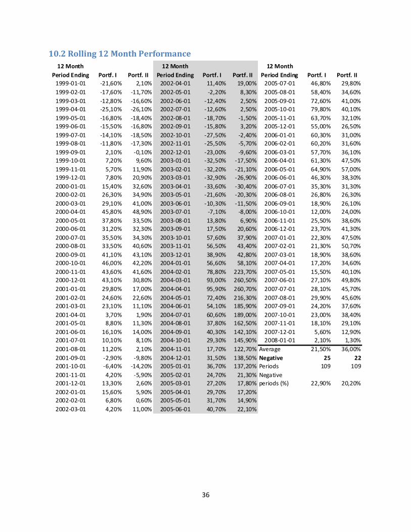
36

10.2 Rolling 12 Month Performance

12 Month

Period Ending Portf. I Portf. II

12 Month


12 Month


1999-01-01 -21,60% 2,10% 2002-04-01 11,40% 19,00% 2005-07-01 46,80% 29,80%

1999-02-01 -17,60% -11,70% 2002-05-01 -2,20% 8,30% 2005-08-01 58,40% 34,60%

1999-03-01 -12,80% -16,60% 2002-06-01 -12,40% 2,50% 2005-09-01 72,60% 41,00%

1999-04-01 -25,10% -26,10% 2002-07-01 -12,60% 2,50% 2005-10-01 79,80% 40,10%

1999-05-01 -16,80% -18,40% 2002-08-01 -18,70% -1,50% 2005-11-01 63,70% 32,10%

1999-06-01 -15,50% -16,80% 2002-09-01 -15,80% 3,20% 2005-12-01 55,00% 26,50%

1999-07-01 -14,10% -18,50% 2002-10-01 -27,50% -2,40% 2006-01-01 60,30% 31,00%

1999-08-01 -11,80% -17,30% 2002-11-01 -25,50% -5,70% 2006-02-01 60,20% 31,60%

1999-09-01 2,10% -0,10% 2002-12-01 -23,00% -9,60% 2006-03-01 57,70% 36,10%

1999-10-01 7,20% 9,60% 2003-01-01 -32,50% -17,50% 2006-04-01 61,30% 47,50%

1999-11-01 5,70% 11,90% 2003-02-01 -32,20% -21,10% 2006-05-01 64,90% 57,00%

1999-12-01 7,80% 20,90% 2003-03-01 -32,90% -26,90% 2006-06-01 46,30% 38,30%

2000-01-01 15,40% 32,60% 2003-04-01 -33,60% -30,40% 2006-07-01 35,30% 31,30%

2000-02-01 26,30% 34,90% 2003-05-01 -21,60% -20,30% 2006-08-01 26,80% 26,30%

2000-03-01 29,10% 41,00% 2003-06-01 -10,30% -11,50% 2006-09-01 18,90% 26,10%

2000-04-01 45,80% 48,90% 2003-07-01 -7,10% -8,00% 2006-10-01 12,00% 24,00%

2000-05-01 37,80% 33,50% 2003-08-01 13,80% 6,90% 2006-11-01 25,50% 38,60%

2000-06-01 31,20% 32,30% 2003-09-01 17,50% 20,60% 2006-12-01 23,70% 41,30%

2000-07-01 35,50% 34,30% 2003-10-01 57,60% 37,90% 2007-01-01 22,30% 47,50%

2000-08-01 33,50% 40,60% 2003-11-01 56,50% 43,40% 2007-02-01 21,30% 50,70%

2000-09-01 41,10% 43,10% 2003-12-01 38,90% 42,80% 2007-03-01 18,90% 38,60%

2000-10-01 46,00% 42,20% 2004-01-01 56,60% 58,10% 2007-04-01 17,20% 34,60%

2000-11-01 43,60% 41,60% 2004-02-01 78,80% 223,70% 2007-05-01 15,50% 40,10%

2000-12-01 43,10% 30,80% 2004-03-01 93,00% 260,50% 2007-06-01 27,10% 49,80%

2001-01-01 29,80% 17,00% 2004-04-01 95,90% 260,70% 2007-07-01 28,10% 45,70%

2001-02-01 24,60% 22,60% 2004-05-01 72,40% 216,30% 2007-08-01 29,90% 45,60%

2001-03-01 23,10% 11,10% 2004-06-01 54,10% 185,90% 2007-09-01 24,20% 37,60%

2001-04-01 3,70% 1,90% 2004-07-01 60,60% 189,00% 2007-10-01 23,00% 38,40%

2001-05-01 8,80% 11,30% 2004-08-01 37,80% 162,50% 2007-11-01 18,10% 29,10%

2001-06-01 16,10% 14,00% 2004-09-01 40,30% 142,10% 2007-12-01 5,60% 12,90%

2001-07-01 10,10% 8,10% 2004-10-01 29,30% 145,90% 2008-01-01 2,10% 1,30%

2001-08-01 11,20% 2,10% 2004-11-01 17,70% 122,70% Average 21,50% 36,00%

2001-09-01 -2,90% -9,80% 2004-12-01 31,50% 138,50% Negative 25 22

2001-10-01 -6,40% -14,20% 2005-01-01 36,70% 137,20% Periods 109 109

2001-11-01 4,20% -5,90% 2005-02-01 24,70% 21,30%

2001-12-01 13,30% 2,60% 2005-03-01 27,20% 17,80% 22,90% 20,20%

2002-01-01 15,60% 5,90% 2005-04-01 29,70% 17,20%

2002-02-01 6,80% 0,60% 2005-05-01 31,70% 14,90%

2002-03-01 4,20% 11,00% 2005-06-01 40,70% 22,10%

Negative

periods (%)

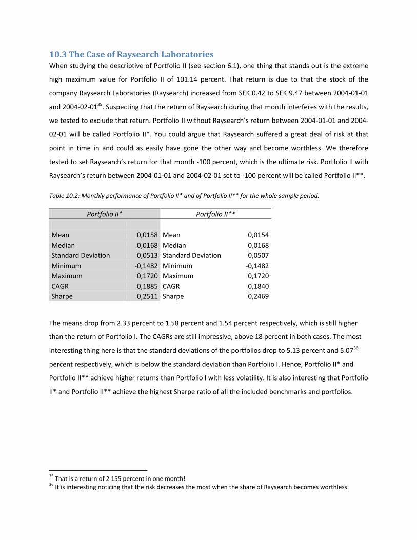
10.3 The Case of Raysearch Laboratories When studying the descriptive of Portfolio II (see section 6.1), one thing that stands out is the extreme

high maximum value for Portfolio II of 101.14 percent. That return is due to that the stock of the

company Raysearch Laboratories (Raysearch) increased from SEK 0.42 to SEK 9.47 between 2004-01-01

and 2004-02-0135. Suspecting that the return of Raysearch during that month interferes with the results,

we tested to exclude that return. Portfolio II without Raysearch’s return between 2004-01-01 and 2004-

02-01 will be called Portfolio II*. You could argue that Raysearch suffered a great deal of risk at that

point in time in and could as easily have gone the other way and become worthless. We therefore

tested to set Raysearch’s return for that month -100 percent, which is the ultimate risk. Portfolio II with

Raysearch’s return between 2004-01-01 and 2004-02-01 set to -100 percent will be called Portfolio II**.

Table 10.2: Monthly performance of Portfolio II* and of Portfolio II** for the whole sample period.

Portfolio II* Portfolio II**

Mean 0,0158 Mean 0,0154





CAGR 0,1885 CAGR 0,1840


The means drop from 2.33 percent to 1.58 percent and 1.54 percent respectively, which is still higher

than the return of Portfolio I. The CAGRs are still impressive, above 18 percent in both cases. The most

interesting thing here is that the standard deviations of the portfolios drop to 5.13 percent and 5.0736

percent respectively, which is below the standard deviation than Portfolio I. Hence, Portfolio II* and

Portfolio II** achieve higher returns than Portfolio I with less volatility. It is also interesting that Portfolio

II* and Portfolio II** achieve the highest Sharpe ratio of all the included benchmarks and portfolios.

35

That is a return of 2 155 percent in one month! 36

It is interesting noticing that the risk decreases the most when the share of Raysearch becomes worthless.

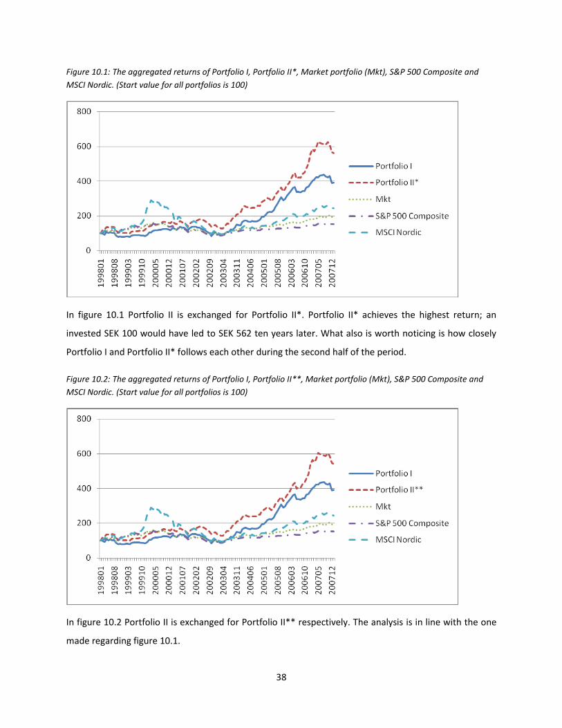
38

Figure 10.1: The aggregated returns of Portfolio I, Portfolio II*, Market portfolio (Mkt), S&P 500 Composite and

MSCI Nordic. (Start value for all portfolios is 100)

In figure 10.1 Portfolio II is exchanged for Portfolio II*. Portfolio II* achieves the highest return; an

invested SEK 100 would have led to SEK 562 ten years later. What also is worth noticing is how closely

Portfolio I and Portfolio II* follows each other during the second half of the period.

Figure 10.2: The aggregated returns of Portfolio I, Portfolio II**, Market portfolio (Mkt), S&P 500 Composite and

MSCI Nordic. (Start value for all portfolios is 100)

In figure 10.2 Portfolio II is exchanged for Portfolio II** respectively. The analysis is in line with the one

made regarding figure 10.1.

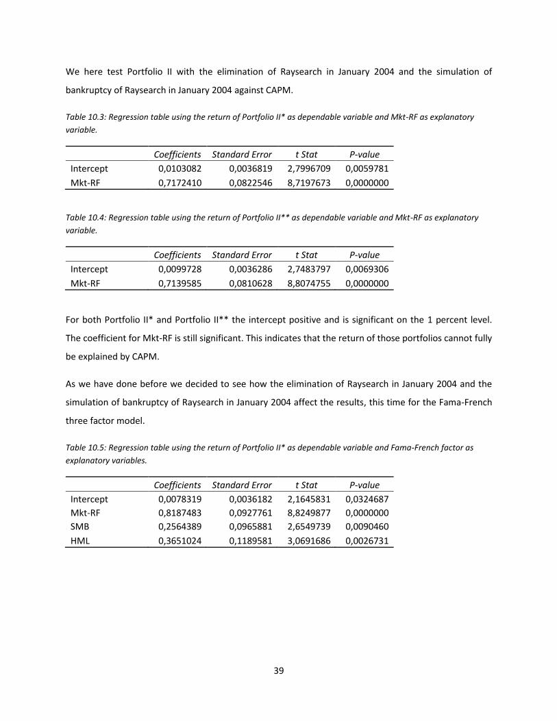
39

We here test Portfolio II with the elimination of Raysearch in January 2004 and the simulation of

bankruptcy of Raysearch in January 2004 against CAPM.

Table 10.3: Regression table using the return of Portfolio II* as dependable variable and Mkt-RF as explanatory

variable.


Intercept 0,0103082 0,0036819 2,7996709 0,0059781

Mkt-RF 0,7172410 0,0822546 8,7197673 0,0000000

Table 10.4: Regression table using the return of Portfolio II** as dependable variable and Mkt-RF as explanatory

variable.


Intercept 0,0099728 0,0036286 2,7483797 0,0069306

Mkt-RF 0,7139585 0,0810628 8,8074755 0,0000000

For both Portfolio II* and Portfolio II** the intercept positive and is significant on the 1 percent level.

The coefficient for Mkt-RF is still significant. This indicates that the return of those portfolios cannot fully

be explained by CAPM.

As we have done before we decided to see how the elimination of Raysearch in January 2004 and the

simulation of bankruptcy of Raysearch in January 2004 affect the results, this time for the Fama-French

three factor model.

Table 10.5: Regression table using the return of Portfolio II* as dependable variable and Fama-French factor as



Intercept 0,0078319 0,0036182 2,1645831 0,0324687

Mkt-RF 0,8187483 0,0927761 8,8249877 0,0000000

SMB 0,2564389 0,0965881 2,6549739 0,0090460

HML 0,3651024 0,1189581 3,0691686 0,0026731

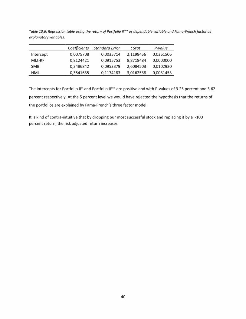
40

Table 10.6: Regression table using the return of Portfolio II** as dependable variable and Fama-French factor as



Intercept 0,0075708 0,0035714 2,1198456 0,0361506

Mkt-RF 0,8124421 0,0915753 8,8718484 0,0000000

SMB 0,2486842 0,0953379 2,6084503 0,0102920

HML 0,3541635 0,1174183 3,0162538 0,0031453

The intercepts for Portfolio II* and Portfolio II** are positive and with P-values of 3.25 percent and 3.62

percent respectively. At the 5 percent level we would have rejected the hypothesis that the returns of

the portfolios are explained by Fama-French’s three factor model.

It is kind of contra-intuitive that by dropping our most successful stock and replacing it by a -100

percent return, the risk adjusted return increases.

41

10.4 Original List of Stock Stock that is marked with an “I” is excluded due to lack of information. Stock that is marked with a “D” is

excluded because there are doublets. Stock that is marked with an “F” is excluded due to being a

financial company. Stock that is marked with an “U” excluded due to being a utility company. Stock that

is unmarked, 744 in total, is a part of the study.

Name of Stock Excluded

AALBORG BOLDSPILKLUB

AARHUS LOKALBANK F

ALM BRAND F

ALM BRAND PANTEBREVE F

ALMANIJ BRAND FORMUE 'B' F

ALK-ABELLO

AMAGERBANKEN F

AMBU

ANDERSEN & MARTINI

A & O JOHANSEN PR.

ARKIL HOLDING

ASGAARD GROUP

ATLANTIC PETROLEUM

AURIGA INDUSTRIES 'B'

BAVARIAN NORDIC

BG INVEST HEALTH CARE I

BG INVEST EUROPA I

IC COMPANYS (EX. UDBYTTE 06/07) I

OSTJYDSK BANK NYE F

BG INVEST VERDEN I

BRONDBY IF 'B'

#ERROR I

BAVARIAN NORDIC NYE I

BANG & OLUFSEN 'B'

BIOPORTO

BOCONCEPT HOLDING 'B'

BONUSBANKEN F

BRD KLEE 'B'

BRODRENE HARTMANN 'B'

CARLSBERG 'B'

CAPINORDIC NYE I

CAPINORDIC F

CARLSBERG 'A' D

CARNEGIE WORLDWIDE I

Name of Stock Excluded

CBRAIN I

CHEMOMETEC I

#ERROR I

COLUMBUS IT PARTNER

#ERROR I

COLOPLAST 'B'

#ERROR I

CURALOGIC

DANSKE BANK F

DANTRUCK

DANIONICS

DANISCO

DANTAX 'B'

DAN EJENDOMME HLDG.

DFDS

DIBA BANK F

DJURSLANDS BANK F

DLH 'B'

#ERROR I

D/S NORDEN

DANTHERM

D/S ORION

A P MOLLER - MAERSK 'A' D

A P MOLLER - MAERSK 'B'

DSV 'B'

D/S TORM

#ERROR I

EUROINVESTOR COM NYE I

EDB GRUPPEN

EGETAEPPER 'B'

EBH BANK A/S F

EUROINVESTOR COM I

EIK BANKI F

ARHUS ELITE 'B'

42

#ERROR I

NORDJYSKE BANK F

ERRIA I

EXIQON NYE I

EXPEDIT 'B'

EXIQON

FE BORDING 'B'

FIRSTFARMS I

FIONIA BANK F

FLSMIDTH & COMPANY 'B'

FLUGGER 'B'

FORSTAEDERNES BANK F

FOROYA BANKI I

FORMUEPLEJE EPIKUR I

FORMUEPLEJE MERKUR I

FORMUEPLEJE PENTA I

FORMUEPLEJE SAFE I

#ERROR I

GABRIEL HOLDING

GENMAB

GREENTECH ENERGY SYS.

GLUNZ & JENSEN

GPV INDUSTRI 'B'

GPV INDUSTRI 'A' D

GRIFFIN III BERLIN 'B' I

GRIFFIN IV BERLIN 'B' I

GRONLANDSBANKEN F

GUDME RAASCHOU VISION I

GN STORE NORD

GREEN WIND ENERGY

GYLDENDAL 'B'

GYLDENDAL 'A' D

HARBOES BRYGGERI 'B'

HEDEGAARD

H&H INTERNATIONAL 'B'

HOJGAARD HLDG.'B'

HOJGAARD HOLDING 'A' D

MAX BANK F

SPAREKASSEN HVETBO I

HVIDBJERG BANK F

IC COMPANYS

INTERMAIL 'B'

INVESTEA GERMAN HIGH ST II I

INVESTEA STOCKHOLM RET. I

JEUDAN

JENSEN & MOL.INVEST

JYSKE BANK F

KAPITALPLEJE F

KOBENHAVNS LUFTHAVNE

KREDITBANKEN F

LAN & SPAR BANK F

LASTAS 'B'

LIFECYCLE PHARMA NYE I

LIFECYCLE PHARMA

FORMUEPLEJE LIMITTELLUS I

LAND & LEISURE 'A' D

LAND & LEISURE 'B'

LOKALBANKEN I NORD F

LOLLANDS BANK F

LUNDBECK

LUXOR 'B'

MACONOMY

MIGATRONIC 'B'

MIDTINVEST I

MONDO I

MONS BANK F

#ERROR I

MOLS-LINIEN

MONBERG & THORSEN 'B'

MORSO BANK F

NEUROSEARCH

NKT

NORDICOM

NORDFYNS BANK F

NORDIC TANKERS

NOVO NORDISK 'B'

NORRESUNDBY BANK F

NORDIC TANKERS NYE I

NETOP SOLUTIONS

NTR HOLDING

NUNAMINERALS I

NOVOZYMES

OLICOM

OSTASIATISKE KOM

OSTJYDSK BANK F

PER AARSLEFF

43

PHARMEXA

PRIME OFFICE I

PARKEN SPORT & ENTM.

ROYAL UNIBREW

RELLA HOLDING

RENEWAGY

RIAS 'B'

RINGKJOBING LNDOBK F

RINGKJOBING BANK F

ROCKWOOL 'A' D

ROBLON 'B'

ROCKWOOL 'B'

ROSKILDE BANK F

ROVSING I

RTX TELECOM

#ERROR I

SALLING BANK F

SANISTAL 'B'

SATAIR

SCANDINAVIAN BRAKE SYS.

SCHOUW & CO

SCF TECHNOLOGIES I

SCHAUMANN PROPERTIES I

DICENTIA

SIF FODBOLD 'B'

SIMCORP

SJAELSOE GRUPPEN

SKJERN BANK NYE I

SKAELSKOR BANK F

SKAKO INDUSTRIES

SKJERN BANK F

SPAR NORD BANK F

SONDAGSAVISEN

SOLAR 'B'

SPAENCOM 'A' D

SPAENCOM 'B'

SPAREKASSEN FAABORG F

SP GROUP

SPAREKASSEN HIMLD. I

SPAREKASSEN LOLLAND I

SPARBANK F

#ERROR I

SVENDBORG SPAREKASSE F

SYDBANK F

TDC

THRANE & THRANE

TIVOLI 'B'

TK DEVELOPMENT

TONDER BANK F

TOPDANMARK F

TOTALBANKEN F

TOWER GROUP

TOPOTARGET

#ERROR I

#ERROR I

DK TRENDS INVEST I

TRIFORK I

TRYGVESTA F

TOPSIL SEMICON.MATS.

UTD.INTL.ENTS.

UNITED PLTNS.AFRICA

UP I

VESTFYNS BANK F

VESTAS WINDSYSTEMS

VIBORG HANDBOLD KLUB 'B'

VICTOR INTERNATIONAL

VINDERUP BANK F

VICTORIA PROPERTIES

VESTJYSK BANK F

VORDINGBORG BANK F

WALLS

WILLIAM DEMANT HLDG.

AFFECTO

AHLSTROM

ALANDSBANKEN 'A' F

ALANDSBANKEN 'B' F

ALDATA SOLUTIONS OYJ

ALMA MEDIA

AMER SPORTS 'A'

UPONOR

ASPOCOMP GROUP

ASPO

ATRIA 'A'

BASWARE

WULFF-GROUP

BIOHIT 'B'

44

BIOTIE THERAPIES

CAPMAN 'B' I

CARGOTEC 'B'

CITYCON

CENCORP

CRAMO

COMPONENTA

COMPTEL

DONE SOLUTIONS

STORA ENSO 'A' D

STORA ENSO 'R'

ELISA

ELCOTEQ SE

ETTEPLAN

EVIA

EXEL

EFORE

FINNLINES

FISKARS 'A' D

FISKARS 'K'

FINNAIR

FORTUM U

F-SECURE

GEOSENTRIC

GLASTON

HEX 25 I

HKSCAN 'A'

HONKARAKENNE 'B'

HUHTAMAKI

ILKKA 1 D

ILKKA YHTYMA

INCAP

INTERAVANTI

ELEKTROBIT

JULIUS TALLBERG

SUOMINEN

KONECRANES

KEMIRA

KESKISUOMALAINEN

KESKO 'A' D

KESKO 'B'

KESLA 'A'

KONE 'B'

LANNEN TEHTAAT

LAROX 'B'

LEMMINKAINEN

LASSILA & TIKANOJA

MARTELA 'A'

MARIMEKKO

METSO

M-REAL 'A' D

M-REAL 'B'

NORDEA BANK FDR F

NESTE OIL

NURMINEN LOGISTICS

#ERROR I

NOKIA

NOKIAN RENKAAT

NORDIC ALUMINIUM

ORIOLA-KD 'A' D

ORIOLA-KD 'B'

OKMETIC

ORAL HAMMASLAAKARIT

ORION 'A' D

ORION 'B'

OUTOTEC

OUTOKUMPU 'A'

OLVI 'A'

PANOSTAJA 'B' D

PANOSTAJA 'A'

PERLOS

PROHA

PKC GROUP

POHJOLA BANK F

POHJOISKARJALAN

PONSSE

POYRY

QPR SOFTWARE

RAMIRENT

RAPALA VMC

#ERROR I

RAUTE 'A'

RUUKKI GROUP

ROCLA

RAUTARUUKKI 'K'

RAISIO 'K'

45

RAISIO YHTYMA 'V' D

SALCOMP

SAMPO 'A' F

SOPRANO I

SOLTEQ

SPONDA

SRV GROUP

SSH COMMS.SCTY.

STOCKMANN 'A' I

STOCKMANN 'B'

STROMSDAL 'B'

STONESOFT

SSK SUOMEN SAASTAJIEN

SUOMEN TERVEYSTALO

DIGIA

TAKOMA

TAMFELT KANTA D

TAMFELT ETU

TALENTUM

TECHNOPOLIS

TEKLA

TELESTE

TECNOMEN

TIETOENATOR

TIIMARI

WESTEND ICT

TRAINERS' HOUSE

TULIKIVI 'A'

ELECSTER 'A'

TURKISTUOTTAJAT 'C'

UPM-KYMMENE

VAAHTO GROUP 'A' D

VAAHTO GROUP 'K'

VACON

VAISALA 'A'

VIKING LINE

SCANFIL

WARTSILA

#ERROR I

IXONOS

YLEISELEKTRONIIKKA OYJ

YIT

ADRESSEAVISEN

AQUA BIO TECHNOLOGY I

ACTA HOLDING F

ACERGY

ABILITY DRILLING I

AF GRUPPEN 'A'

ARENDALS FOSSEKOMPANI U

ARTUMAS GROUP I

AGR GROUP

AKTIV KAPITAL F

AKER BIOMARINE

AKER

AKER FLOATING PRODUCTION

AKER PHILADELPHIA SHPYD. I

AKER SEAFOODS

AKER SOLUTIONS

AKVA GROUP I

AKER EXPLORATION

AKER YARDS

ALGETA

AMERICAN SHIPPING CO.

APPTIX

ABG SUNDAL CLI.HLDG. F

AURSKOG SPAREBANK F

AUSTEVOLL SEAFOOD

AWILCO OFFSHORE

BELSHIPS

BERGEN GROUP I

BIOTEC PHARMACON

BIRDSTEP TECHNOLOGY

BJORGE

BLOM

BLUEWATER INSURANCE F

BYGGMA

BONHEUR

BORGESTAD 'A'

BOUVET I

BWG HOMES

BW GAS I

BW OFFSHORE

BADGER EXPLORER

CECON I

CAMILLO EITZEN & CO

CERMAQ

46

CLAVIS PHARMA I

CODFARMERS I

COMROD COMMUNICATION I

CONFIRMIT I

COPEINCA

CONTEXTVISION

CAMPOSOL HOLDING I

DATA RESPONS

DEEP SEA SUPPLY

DET NORS.OLJESELSKAP

DIAGENIC

DNB NOR F

DNO INTERNATIONAL

DOCKWISE

DOF

DOF SUBSEA

DOLPHIN INTCONN.SLN. I

DOMSTEIN

EITZEN CHEMICAL

EDB BUSINESS PARTNER

EIDSIVA REDERI

EIDESVIK OFFSHORE

EKORNES

ELTEK

EMENTOR

ELECTROMAGNETIC GEOSVS.

EITZEN MARITIME SERVICES

EOC

ETMAN INTERNATIONAL I

EXENSE

EXENSE CONSULTING DEAD - 24/09/08 I

FAIRSTAR HEAVY TRAN.

FAKTOR EIENDOM I

FARSTAD SHIPPING

FARA ASA

FRED OLSEN ENERGY

FRED OLSEN PRDN.

FOSEN

FRONTLINE

FUNCOM

GRENLAND GROUP ASA

GLOBAL GEO SERVICES

GLOBAL IP SLTN.HOLDING I

GOODTECH

GOLDEN OCEAN GROUP

GOLAR LNG

GREGOIRE I

GANGER ROLF

GREEN REEFERS

GRIEG SEAFOOD I

GYLDENDAL

HAVILA ARIEL I

HAVILA SHIPPING

HELGELAND SPAREBANK I

HEXAGON COMPOSITES

HAFSLUND INFRATEK I

HJELLEGJERDE

HAFSLUND 'A' U

HAFSLUND 'B' U

HOL SPAREBANK F

HURTIGRUTEN

HOLAND SPAREBANK I

INTERNATIONAL GOLD EXP.

IGE NORDIC I

IGNIS

IMAREX F

IM SKAUGEN

INMETA

INVIVOSENSE I

INTEROIL EXP.& PRDN. I

INDRE SOGN SPAREBANK F

INTELECOM GROUP

ITERA CONSULTING GROUP

INTEX RESOURCES

PETROJACK

JINHUI SHIP.& TRSP.

KONGSBERG AUTV.HOLDING

KITRON

KLEPP SPAREBANK I

KONGSBERG GRUPPEN

KOMPLETT

KVERNELAND

LIGHTHOUSE CALEDONIA

LONDON MINING I

LEROY SEAFOOD GROUP

LUXO

47

MARINE FARMS I

MAMUT

MEDICULT

MEDI-STIM

MELHUS SPAREBANK F

MARINE HARVEST

SPAREBANK 1 SMN F

MARITIM INDUSTRIAL SVS.

SPAREBANKEN MORE F

NAMSOS TRAFIKKSELSKAP

NORWEGIAN AIR SHUTTLE

NATTOPHARMA I

NAVAMEDIC I

NEAS I

NORSE ENERGY CORP.

NES PRESTEGJELDS SPB. F

NEXUS FLOATING PRDN. I

NORSK HYDRO

NIO SECURITY I

NORTHERN LOGISTIC PR.

NORDIC SEMICONDUCTOR

NORWEGIAN ENERGY CO.

NORDIC MINING I

SPAREBANK 1 NORD-NORGE F

NORWEGIAN PROPERTY

NORMAN

NORDIAG ASA

NORWAY PELAGIC I

NORSKE SKOG

SPAREBANK 1 NOTTEROY I

NUTRIPHARMA

ODFJELL 'A' D

ODFJELL 'B'

ODIM

OCEAN HEAVY LIFT

ODFJELL INVEST

OLAV THON

OPERA SOFTWARE

OCEANTEAM I

ORKLA

OTRUM

PCI BIOTECH HOLDING I

PETROLIA DRILLING

PETROLEUM GEO SERVICES

PHOTOCURE

SPAREBANKEN PLUSS F

PETROMENA

POWEL

PETROPROD I

PROSAFE PRODUCTION PUB. I

PRONOVA BIOPHARMA

PROTECTOR FORSIKRING I

PROSAFE

PSI GROUP

Q-FREE

RENEWABLE ENERGY

REM OFFSHORE

REPANT I

REVUS ENERGY

ROCKSOURCE

RIEBER & SON

RINGERIKE SPAREBANK F

GC RIEBER SHIPPING

REMEDIAL (CYPRUS) I

SPAREBANK 1 SR BANK F

ROMREAL I

ROXAR

RYGGE-VAALER SPB I

RESERVOIR EXP.TECH.'B'

SANDNES SPAREBANK F

SALMAR

SANDSVAER SPAREBANK F

SEABIRD EXPLORATION

SCANARC

SCAN GEOPHYSICAL

SCHIBSTED

SCANA INDUSTRIER

SCANDINAVIAN CLIN.NUT. I

SCORPION OFFSHORE

SEADRILL

SEAJACKS INTERNATIONAL

SEVAN MARINE

SYNNOVE FINDEN

SIMTRONICS I

SIEM OFFSHORE

SIMRAD OPTRONICS

48

SKIENS AKTIEMOLLE

STOLT NIELSEN

SOLSTAD OFFSHORE

SOFTWARE INNOVATION

SOLVANG

SONGA OFFSHORE

SCANDINAVIAN PR.DEV.

SPAREBANKEN OST F

SPECTRUM I

STAR REEFERS

STAVANGER AFTENBLAD

STOREBRAND F

STATOILHYDRO

STEPSTONE

SUBSEA 7

SUPEROFFICE

SPAREBANKEN VEST F

TANDBERG

TANDBERG DATA

TELECOMPUTING

TECO MARITIME

TELENOR

TELIO HOLDING I

24SEVENOFFICE

TGS-NOPEC GEOPHS.

THIN FILM ELECTRONICS I

THULE DRILLING I

TIDE

TOMRA

TOTENS SPAREBANK F

TANDBERG STORAGE

TTS MARINE

VEIDEKKE

VMETRO

SPAREBANKEN VESTFOLD F

VOSS VEKSEL-OG LMDBK. F

WAVEFIELD INSEIS

WEGA MINING

WILSON

WILHS.WILHELMSEN 'A' D

WILHS.WILHELMSEN 'B'

YARA INTERNATIONAL

ZONCOLAN I

2ENTERTAIN

360 HOLDING I

3L SYSTEM

AARHUSKARLSHAMN

ACAP INVEST 'A' I

ACADEMEDIA 'B'

ACANDO 'B'

ACAP INVEST I

ATLAS COPCO 'B'

ACCELERATOR NORDIC 'B'

ACSC DEAD - 31/12/07

ACTIVE BIOTECH

ADDVISE

ADDTECH 'B'

AEROCRINE 'B'

AF 'B'

AFFARSSTRATEGERNA 'B'

AGELLIS GROUP I

AIK FOTBOLL 'B'

ALFA LAVAL

AUTOLIV SDB I

BEIJER ALMA 'B'

ALLOKTON 'B' I

ALPHAHELIX MOLEDIAG.

AMAGO CAPITAL I

AMHULT 2 'B'

ANCORA ENERGISPAR I

ANNEHEM FASTIGHETER I

ADDNODE 'B'

ANOTO GROUP

AROS QUALITY GROUP

AQERI HOLDING I

ARCAM 'B'

ARENA PERSONAL I

ARK TRAVEL

ARTIMPLANT

ASPIRO

ASSA ABLOY 'B'

ALLTELE ALLM.SVEN.TELAB I

AQUA TERRENA

AUDIODEV 'B'

AU HOLDING

AVALON ENTERPRISE 'B'

49

AVEGA I

AVENSIA INNOVATION

AVONOVA SVERIGE

AXFOOD

AXIS

AXLON GROUP I

AVANZA BANK HOLDING F

BAHNHOF 'B' I

FASTIGHETS BALDER 'B'

BALLINGSLOV INTL.

B&B TOOLS 'B'

BE GROUP

BEIJER ELECTRONICS

BEOWULF MINING SDB I

BETSSON 'B'

BETTING PROM.SWEDEN

BONG LJUNGDAHL

BIOSENSOR APPS.SWEDEN 'A'

BIOGAIA 'B'

BILIA 'A'

BILLERUD

BIOINVENT INTL.

BIOMETRON 'B'

BIOPHAUSIA 'A'

BIOTAGE

BJORN BORG

ELEKTRONIKGRUPPEN BK 'B'

BLACK EARTH FARMING SDB

BENCHMARK OIL & GAS

BOLIDEN

BOREVIND

BRIO 'B'

BERGS TIMBER 'B'

BRINOVA FASTIGHETER

BROSTROM

BRIO 'B' SPECIAL RIGHTS I

BTS GROUP

BURE EQUITY

BIOVITRUM

BRINGWELL INTERNATIONAL

C2SAT 'B' I

CENTRAL ASIA GOLD I

NCS NDC.CAMPING & SPS.

CATERING PLEASE I

CAPILON I

D CARNEGIE & CO F

CARDO

CARL LAMM I

CASTELLUM

CATENA

CATECH 'B' I

CYBAERO I

COMMUNITY ENTM. I

CELLAVISION I

CHEMEL I

CHERRYFORETAGEN 'B' I

CLAS OHLSON 'B'

CARL LAMM HOLDING I

CONCORDIA MARITIME 'B'

CISION

CONNECTA

CONPHARM 'A' D

CONPHARM 'B'

SVENSKA CAPITAL OIL I

A-COM

CONSILIUM 'B'

CONFIDENCE INTL.'B'

COOLGUARD 'B'

COREM PROPERTY GROUP I

COUNTERMINE 'B' I

CELLPOINT CONNECT

C-RAD 'B' I

CLOETTA FAZER 'B'

CTT SYSTEMS

CYBERCOM GROUP EUROPE

CRYPTZONE I

DACKE GROUP NORDIC I

DAGON

DEVICOM I

DGC ONE I

DIADROM HOLDING I

DIAMYD MEDICAL 'B'

DTG SWEDEN I

DIBS PAYMENT SER. I

DIN BOSTAD SVERIGE

DIOS FASTIGHETER I

50

DANNEMORA MINERAL I

DO NETWORKS SVERIGE I

#ERROR I

DONE MAN.& SYS. I

DORO

DRILLCON I

DUROC 'B'

DUNI

DIGITAL VISION

ELECTROLUX 'A'

EAST CAPITAL EXPLORER F

EIRIKUVA DIGITAL IMAGE I

EDI COMPANY 'B' I

EFFNET HOLDING

HEXAGON 'B'

ELECTRA GRUPPEN I

ELEKTA 'B'

ELLEN I

ELANDERS 'B'

ELOS 'B'

ELVERKET VALLENTUNA U

EMPIRE 'B'

EMITOR HOLDING I

ENACO

ENEA

ENDOMINES

#ERROR I

ENLIGHT INTERNATIONAL

ENJOY GROUP 'B' I

ENIRO

ENTRACTION HOLDING 'B'

ENERGYO SLTN.RUSSIA I

ERICSSON 'A'

EUROCINE VACCINES

EUROCON CONSULTING I

EUROPEAN INST.OF SCI.'B'

EUROVIP GROUP 'A' I

EUROVIP GROUP 'B' I

FABEGE

FAGERHULT

FAST PARTNER

FASTTV NET

FEELGOOD SVENSKA

FINGERPRINT CARDS

FIREFLY

FENIX OUTDOOR

FORSSTROM HIGH FREQ.

FOLLOWIT HOLDING

FORSHEM GROUP I

FORMPIPE SOFTWARE I

FRAGUS GROUP 'B'

FUNDIOR I

GEVEKO 'B'

GENERIC SWEDEN I

GENLINE HOLDING

GENOVIS 'B'

GLOBALFUN I

GLOBAL GAMING FACTORY X

GIFTTODAY SWEDEN

GETUPDATED INET.MKTG.

GETINGE

GUIDELINE OIL DRL.TECH. I

LAPPLAND GOLDMINERS

GLYCOREX TRANSPL 'B'

GULD INVEST NORDEN I

GUNNEBO INDUSTRIER

GUNNEBO

GEXCO I

H1 COMMUNICATION 'B' I

HAKON INVEST

HALDEX

HAMMAR INVEST 'B'

HUFVUDSTADEN 'C'

HEBA 'B'

HEBI HEALTH CARE I

HEDSON TECHS.INTL.

HEMTEX

HIQ INTERNATIONAL

HL DISPLAY 'B'

PEAB 'B'

HENNES & MAURITZ 'B'

HANSA MEDICAL I

HMS NETWORKS I

HEART OF BRANDS 'B' I

HOGANAS 'B'

HOMEMAID

51

HOME PROPERTIES

HEXPOL 'B' I

HQ F

HUFVUDSTADEN 'A' I

HUMAN CARE H C

HUSQVARNA 'A' D

HUSQVARNA 'B'

IBS 'B'

ICT SWEDEN HOLDING I

ICM KUNGSHOLMS

INTELLECTA 'B'

IDL BIOTECH 'B'

INDL.& FINL.SYS.'A' D

INDL.& FINL.SYS.'B'

#ERROR I

IMPACT COATINGS I

INDUTRADE

INTRUM JUSTITIA

INNATE PHARMS.'A'

INTOI

INTIUS

INVESTOR 'A' D

INSPLANET I

INVESTOR 'B'

ITAB SHOP CONCEPT 'B'

INDUSTRIVARDEN 'A' D

INDUSTRIVARDEN 'C'

INVISIO HEADSETS I

RORVIK TIMBER

JAMES CONCEPTS I

JEEVES INFO.SYSTEMS

JELLO

JLT MOBILE COMPUTERS

JM

KARO BIO

KAPPAHL HOLDINGS

KABE HUSVAGNAR 'B'

KONTAKT EAST HOLDING I

KINNEVIK 'A' D

KINNEVIK 'B'

KLOVERN

KUNGSLEDEN

KLICK DATA 'B'

#ERROR I

KOPPARBERG MINERAL 'B' I

KNOW IT

KINDWALLS 'B'

LABS2GROUP

LAGERCRANTZ 'B'

LAMMHULTS DESIGN GROUP

LBI INTERNATIONAL

LINDAB INTERNATIONAL

LIFEASSAYS 'B' I

LINEAR 'B'

#ERROR I

ATRIUM LJUNGBERG 'B'

LINKMED I

LUNDBERGFORETAGEN 'B'

LOVISAGRUVAN I

LATOUR INVESTMENT 'A' D

LATOUR INVESTMENT 'B'

LUCENT OIL

LUNDIN MINING SDB I

LUNDIN PETROLEUM

MAHLER INTERNATIONAL AB

MALKA OIL I

MEDCAP I

MICRO HOLDING

MEDIVIR 'B'

MIDWAY HOLDINGS 'A' D

MALMBERGS ELEKTRISKA

MEDA 'A'

BIOLIN

MEGACON

MEKONOMEN

MELKER SCHORLING

MEDIAPROVIDER SCAN. I

MICRONIC LASER SYS.

MILLICOM INTL.CELU.SDB I

MIDWAY HOLDINGS 'B'

MIRIS HOLDING

MUNTERS

#ERROR I

MOBISPINE I

MOBYSON

HOLMEN 'A'

52

MODUL 1 DATA

MORPHIC TECHNOLOGIES 'B'

MODERN TIMES GP.MTG 'A' D

MODERN TIMES GP.MTG 'B'

MEDICPEN

MEDIROX 'A' I

MICRO SYSTEMATION 'B' I

MSC KONSULT 'B'

MIDELFART SONESSON 'B'

MIDELFART SONESSON 'A' D

METRO INTL.SDB 'B'

METRO INTL.SDB 'A' D

MULTIQ INTERNATIONAL

MYSCOOP INTERNATIONAL I

NOLATO 'B'

NORDIC ACS.BUYOUT FUND I

NOVACAST TECHS.'B'

NORDEA BANK F

NEONET

NET ENTERTAINMENT NE 'B'

NET INSIGHT 'B'

NETREVELATION

NEW WAVE GROUP 'B'

TECHNOLOGY NEXUS

NGM HOLDING I

NGS NEXT GENERATION SYS. SWEDEN I

NIBE INDUSTRIER 'B'

NILORNGRUPPEN 'B'

NISCAYAH GROUP 'B'

NEDERMAN HOLDING

NEW NORDIC HEALTHBRANDS I

NOBIA

NORDIC MINES I

NETONNET

NOTE

NOVOTEK 'B'

NOVUS GROUP INTL.

NORDNET SECURITIES BANK F

NORDIC SER.PTNS.HDG.'B' I

NCC 'A' D

NCC 'B'

OASMIA PHARMACEUTICAL I

OBDUCAT 'B'

ODD MOLLY INTL. I

ODEN CONTROL 'B'

OEM INTERNATIONAL 'B'

ONSKEFOTO I

OPCON

OPUS PRODOX I

ORC SOFTWARE

ORIFLAME COSMETICS SDB

ORTIVUS 'A' D

ORTIVUS 'B'

OREXO

ORASOLV I

PANALARM I

PA RESOURCES 'B'

PARTNERTECH

PANAXIA SECURITY I

PAYNOVA I

PRECOMP SOLUTIONS 'B' I

PARADOX ENTERTAINMENT I

PHONERA

PILUM 'B' I

PEAB INDUSTRI 'B'

POLYPLANK I

POOLIA 'B'

PROBI

PRECIO SYSTEMUTVECKLING

PROACT IT GROUP

PREVAS 'B'

PRECISE BIOMETRICS

PRICER 'B'

PROFFICE 'B'

PROFILGRUPPEN 'B'

PUSH DEVELOPMENT I

PV ENTERPRISE SWEDEN

PEARL EXP.& PRDN.SDB. I

Q-MED

RATOS 'A' D

REDERI AB TNSAT.'B'

RAILCARE GROUP I

RASTA GROUP

RELATION AND BRAND 'B'

REDBET HOLDING I

RAYCLINIC I

53

REJLERKONCERNEN 'B' I

RESURS CNC 'B' I

REZIDOR HOTEL GROUP

RADIO FREQ.INV.GP.SWEDEN

RAYSEARCH LABORATORIES

ROTTNEROS

RNB RETAIL AND BRANDS

READSOFT 'B'

RATOS 'B'

RUNAWARE I

RUSSIAN RL.EST.INV.

SAAB 'B'

SAFE AT SEA I

SAGAX I

SANDVIK

SAS

SVERIGES BOSTADSRATTSCENTRUM

SCA 'A' D

SCRIBONA 'A' D

SCRIBONA 'B'

SCIROCCO 'B'

SWITCHCORE

#ERROR I

SCANIA 'A' D

SCANIA 'B'

SEAMLESS DISTRIBUTION I

ELECTROLUX 'B' D

SEB 'A' F

SEANET MARITIME COMMS. I

SEMCON

SEB 'C' F

SENSYS TRAFFIC

SWEDE RESOURCES

SERVAGE 'B' I

SECTRA 'B'

SENZIME I

SKANDITEK INDRI.FRV.

SVENSKA HANDBKN.'B' F

SIGMA B

SINTERCAST

SV.INTERNETREKRYTERING I

SIX 'B'

SJR IN SCANDINAVIA 'B' I

SKANE MOLLAN

SKANSKA 'B'

SKF 'A' D

SKF 'B'

SKISTAR 'B'

G & L BEIJER

ERICSSON 'B' D

HOLMEN 'B' D

SMARTEQ 'B'

SECO TOOLS 'B'

SOFTRONIC 'B'

PSI SPELINVEST I

ATLAS COPCO 'A' D

SRAB SHIPPING 'B'

SSAB 'A' D

SSAB 'B'

STARBREEZE

STAVRULLEN FINANS 'B' I

STORA ENSO 'A' (OME) I

STORA ENSO 'R' (OME) I

STILLE

STRAND INTERCONNECT 'A' D

STRAND INTERCONNECT 'B'

1618 STRICT B SHARE I

STORMFAGELN

STAR VAULT I

SECURITAS 'B'

SVEDBERGS 'B'

STUDSVIK

SVITHOID TANKERS 'B' I

SVENSKA HANDBKN.'A' F

SCA 'B'

SWECO 'A' D

SWECO 'B'

SWEDBANK 'A' F

SWEDISH MATCH

SWEDOL 'B'

SY.SEPTN.SWEDEN HLDG.

SYSTEMAIR

TRIGON AGRI

TATURA I

TAURUS ENERGY 'B' I

TELE2 'B'

54

TELE2 'A' D

TELECA 'B'

#ERROR I

TETHYS OIL I

TAGMASTER I

TELIGENT

THALAMUS NETWORKS 'B'

TICKET TRAVEL

TILGIN I

TELIASONERA

TOWORK SVERIGE I

TRAVELPARTNER I

TRIPEP I

TRADEDOUBLER

TRACTECHNOLOGY

#ERROR I

TRIMERA

TRICORONA F

TRETTI I

SKY COMMUNICATION

TRELLEBORG 'B'

TRANSCOM WWD.SDB.A D

TRANSCOM WWD.SDB.B

TANGANYIKA OIL SDB I

UNIFLEX 'B' I

ULYSS I

UNIBET GROUP SDB

UNLTD.TRAVEL GROUP I

VARYAG RESOURCES I

VOSTOK GAS SDB

VBG GROUP

VICTORIA PARK I

VINOVO I

VITEC SOFTWARE GROUP 'B'

VITROLIFE

VARMEKYL GRSSN.SCAN.

VLT 'B'

VOSTOK NAFTA INV.SDB

VITA NOVA VENTURES

VOLVO 'B'

VOLVO 'A' D

BORAS WAFVERI 'B'

WAYFINDER SYSTEMS I

WALLENSTAM 'B'

WEDINS SKOR & ACESOR.'B'

WESC I

#ERROR I

WIHLBORGS FASTIGHETER

WIKING MINERAL

WEST INTERNATIONAL I

WISE GROUP I

WATER JET SWEDEN I

WHITE SHARK 'B' I

WEST SIBERIAN RES.SDB

XANO INDUSTRI 'B'

XTRACOM CNSL.GROUP 'B' I

XPONCARD

XRF ANALYTICAL 'B' I

XTRANET

ZODIAK TELEVISION 'B'

ATLANTIC AIRWAYS (ICE) I

HF EIMSKIPAFELAG ISLANDS

BAKKAVOR

EXISTA F

FL GROUP DEAD - 09/06/08

GRANDI HF I

HAMPIDJAN I

ICELANDAIR GROUP

GLITNIR BANKI F

ATORKA GROUP

KAUPTHING BANK F

LANDSBANKI ISLANDS F

MAREL FOOD SYSTEMS

NYHERJI I

OSSUR

ALFESCA

SKIPTI HF I

SLATURFELAG SUDURLAND I

SPRON I

STRAUMUR BUROARAS F

TEYMI I

TRYGGINGAMIDSTODIN HF F

VINNSLUSTODIN I

55

10.5 The Stocks Selected in Each Period

Date Portfolio I

1998-01-01 SPAENCOM ACTIVE BIOTECH

1998-02-01 OSTASIATISKE KOM PANOSTAJA

1998-03-01 SOLAR BURE EQUITY

1998-04-01 TURKISTOUTTAJAT RAUTE

1998-05-01 G&L BEIJER BEIJER ALMA 'B'

1998-06-01 GC RIEBER SHIPPING FLÜGGER

1998-07-01 ARKIL HOLDING TOWER GROUP

1998-08-01 EVIA SKANSKA 'B'

1998-09-01 HEXAGON ORKLA

1998-10-01 VOLVO 'B' TULIKIVI

1998-11-01 INTELLECTA 'B' LAROX

1998-12-01 SANISTAL A&O JOHANSEN

1999-01-01 EXPEDIT GLUNZ & JENSEN

1999-02-01 GPV INDUSTRI MARTELA

1999-03-01 BONHEUR LEMMINKAINEN

1999-04-01 TURKISTOUTTAJAT OSTASIATISKE KOM

1999-05-01 GANGER ROLF SKAKO INDUSTRIES

1999-06-01 RENEWAGY FLÜGGER

1999-07-01 ELECTROLUX 'A' MONBERG & THORSEN 'B'

1999-08-01 GC RIEBER SHIPPING TOWER GROUP

1999-09-01 INCAP GABRIEL HOLDING

1999-10-01 LANNEN TEHAT BURE EQUITY

1999-11-01 OLICOM TULIKIVI

1999-12-01 IC COMPANYS A&O JOHANSEN

2000-01-01 PANOSTAJA SANISTAL

2000-02-01 MARTELA SCANA INDUSTRIER

2000-03-01 NKT SOLAR

2000-04-01 LEMMIKAINEN GEVEKO

2000-05-01 RAUTE AURIGA INDUSTRIES

2000-06-01 KESLA INDUSTRIVARDEN 'C'

2000-07-01 ELECTROLUX 'A' FLÜGGER

2000-08-01 WARTSILA CARDO

2000-09-01 SKANSKA 'B' STOCKMANN

2000-10-01 SKF 'B' SECO TOOLS 'B'

2000-11-01 HALDEX HONKARAKENNE

2000-12-01 OLICOM GABRIEL HOLDING

2001-01-01 PANOSTAJA A&O JOHANSEN

2001-02-01 MARTELA TURKISTOUTTAJAT

2001-03-01 ADDNODE MONBERG & THORSEN 'B'

2001-04-01 SCHOUW & CO TRAINERS' HOUSE

2001-05-01 AF VLT 'B'

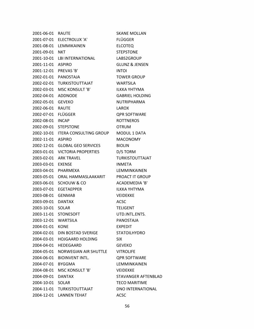
56

2001-06-01 RAUTE SKANE MOLLAN

2001-07-01 ELECTROLUX 'A' FLÜGGER

2001-08-01 LEMMIKAINEN ELCOTEQ

2001-09-01 NKT STEPSTONE

2001-10-01 LBI INTERNATIONAL LABS2GROUP

2001-11-01 ASPIRO GLUNZ & JENSEN

2001-12-01 PREVAS 'B' INTOI

2002-01-01 PANOSTAJA TOWER GROUP

2002-02-01 TURKISTOUTTAJAT WARTSILA

2002-03-01 MSC KONSULT 'B' ILKKA YHTYMA

2002-04-01 ADDNODE GABRIEL HOLDING

2002-05-01 GEVEKO NUTRIPHARMA

2002-06-01 RAUTE LAROX

2002-07-01 FLÜGGER QPR SOFTWARE

2002-08-01 INCAP ROTTNEROS

2002-09-01 STEPSTONE OTRUM

2002-10-01 ITERA CONSULTING GROUP MODUL 1 DATA

2002-11-01 ASPIRO MACONOMY

2002-12-01 GLOBAL GEO SERVICES BIOLIN

2003-01-01 VICTORIA PROPERTIES D/S TORM

2003-02-01 ARK TRAVEL TURKISTOUTTAJAT

2003-03-01 EXENSE INMETA

2003-04-01 PHARMEXA LEMMINKAINEN

2003-05-01 ORAL HAMMASLAAKARIT PROACT IT GROUP

2003-06-01 SCHOUW & CO ACADEMEDIA 'B'

2003-07-01 EGETAEPPER ILKKA YHTYMA

2003-08-01 GENMAB VEIDEKKE

2003-09-01 DANTAX ACSC

2003-10-01 SOLAR TELIGENT

2003-11-01 STONESOFT UTD.INTL.ENTS.

2003-12-01 WARTSILA PANOSTAJA

2004-01-01 KONE EXPEDIT

2004-02-01 DIN BOSTAD SVERIGE STATOILHYDRO

2004-03-01 HOJGAARD HOLDING SIX

2004-04-01 HEDEGAARD GEVEKO

2004-05-01 NORWEGIAN AIR SHUTTLE VITROLIFE

2004-06-01 BIOINVENT INTL. QPR SOFTWARE

2004-07-01 BYGGMA LEMMINKAINEN

2004-08-01 MSC KONSULT 'B' VEIDEKKE

2004-09-01 DANTAX STAVANGER AFTENBLAD

2004-10-01 SOLAR TECO MARITIME

2004-11-01 TURKISTOUTTAJAT DNO INTERNATIONAL

2004-12-01 LANNEN TEHAT ACSC

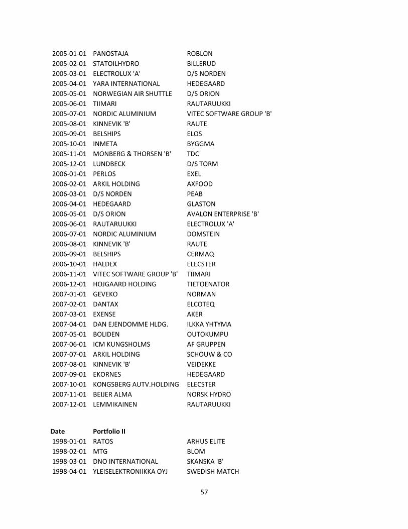
57

2005-01-01 PANOSTAJA ROBLON

2005-02-01 STATOILHYDRO BILLERUD

2005-03-01 ELECTROLUX 'A' D/S NORDEN

2005-04-01 YARA INTERNATIONAL HEDEGAARD

2005-05-01 NORWEGIAN AIR SHUTTLE D/S ORION

2005-06-01 TIIMARI RAUTARUUKKI

2005-07-01 NORDIC ALUMINIUM VITEC SOFTWARE GROUP 'B'

2005-08-01 KINNEVIK 'B' RAUTE

2005-09-01 BELSHIPS ELOS

2005-10-01 INMETA BYGGMA

2005-11-01 MONBERG & THORSEN 'B' TDC

2005-12-01 LUNDBECK D/S TORM

2006-01-01 PERLOS EXEL

2006-02-01 ARKIL HOLDING AXFOOD

2006-03-01 D/S NORDEN PEAB

2006-04-01 HEDEGAARD GLASTON

2006-05-01 D/S ORION AVALON ENTERPRISE 'B'

2006-06-01 RAUTARUUKKI ELECTROLUX 'A'

2006-07-01 NORDIC ALUMINIUM DOMSTEIN

2006-08-01 KINNEVIK 'B' RAUTE

2006-09-01 BELSHIPS CERMAQ

2006-10-01 HALDEX ELECSTER

2006-11-01 VITEC SOFTWARE GROUP 'B' TIIMARI

2006-12-01 HOJGAARD HOLDING TIETOENATOR

2007-01-01 GEVEKO NORMAN

2007-02-01 DANTAX ELCOTEQ

2007-03-01 EXENSE AKER

2007-04-01 DAN EJENDOMME HLDG. ILKKA YHTYMA

2007-05-01 BOLIDEN OUTOKUMPU

2007-06-01 ICM KUNGSHOLMS AF GRUPPEN

2007-07-01 ARKIL HOLDING SCHOUW & CO

2007-08-01 KINNEVIK 'B' VEIDEKKE

2007-09-01 EKORNES HEDEGAARD

2007-10-01 KONGSBERG AUTV.HOLDING ELECSTER

2007-11-01 BEIJER ALMA NORSK HYDRO

2007-12-01 LEMMIKAINEN RAUTARUUKKI Date Portfolio II

1998-01-01 RATOS ARHUS ELITE

1998-02-01 MTG BLOM

1998-03-01 DNO INTERNATIONAL SKANSKA 'B'

1998-04-01 YLEISELEKTRONIIKKA OYJ SWEDISH MATCH

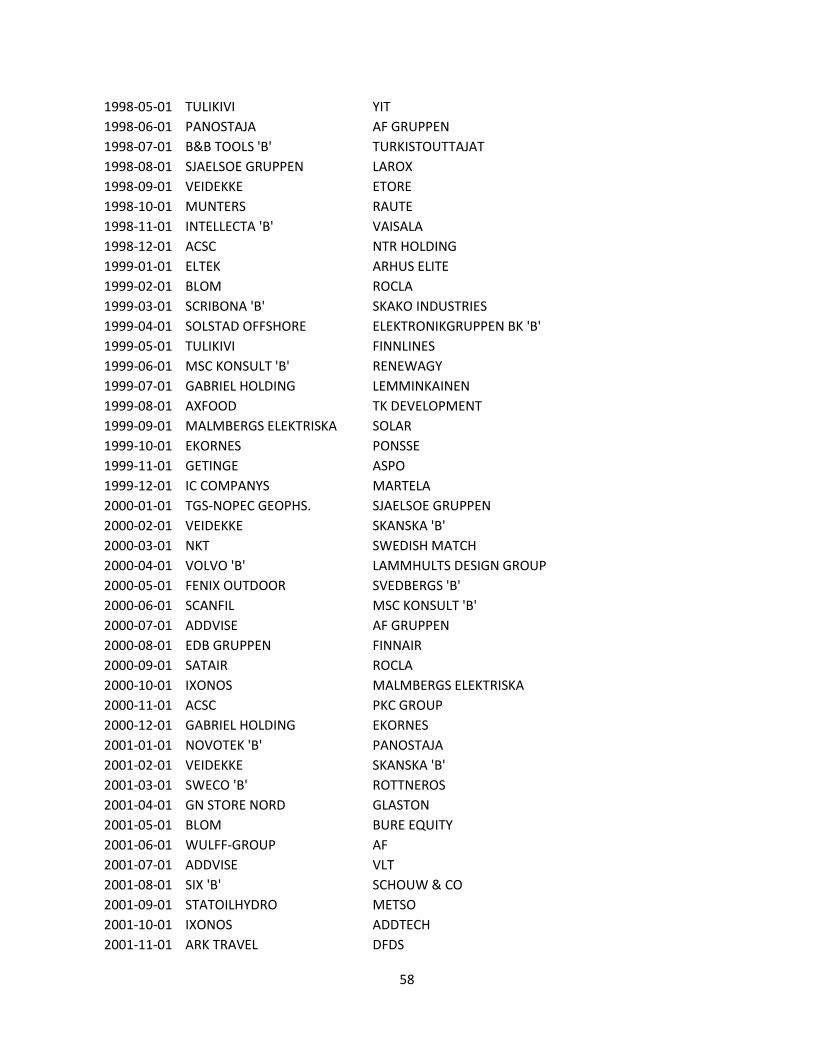
58

1998-05-01 TULIKIVI YIT

1998-06-01 PANOSTAJA AF GRUPPEN

1998-07-01 B&B TOOLS 'B' TURKISTOUTTAJAT

1998-08-01 SJAELSOE GRUPPEN LAROX

1998-09-01 VEIDEKKE ETORE

1998-10-01 MUNTERS RAUTE

1998-11-01 INTELLECTA 'B' VAISALA

1998-12-01 ACSC NTR HOLDING

1999-01-01 ELTEK ARHUS ELITE

1999-02-01 BLOM ROCLA

1999-03-01 SCRIBONA 'B' SKAKO INDUSTRIES

1999-04-01 SOLSTAD OFFSHORE ELEKTRONIKGRUPPEN BK 'B'

1999-05-01 TULIKIVI FINNLINES

1999-06-01 MSC KONSULT 'B' RENEWAGY

1999-07-01 GABRIEL HOLDING LEMMINKAINEN

1999-08-01 AXFOOD TK DEVELOPMENT

1999-09-01 MALMBERGS ELEKTRISKA SOLAR

1999-10-01 EKORNES PONSSE

1999-11-01 GETINGE ASPO

1999-12-01 IC COMPANYS MARTELA

2000-01-01 TGS-NOPEC GEOPHS. SJAELSOE GRUPPEN

2000-02-01 VEIDEKKE SKANSKA 'B'

2000-03-01 NKT SWEDISH MATCH

2000-04-01 VOLVO 'B' LAMMHULTS DESIGN GROUP

2000-05-01 FENIX OUTDOOR SVEDBERGS 'B'

2000-06-01 SCANFIL MSC KONSULT 'B'

2000-07-01 ADDVISE AF GRUPPEN

2000-08-01 EDB GRUPPEN FINNAIR

2000-09-01 SATAIR ROCLA

2000-10-01 IXONOS MALMBERGS ELEKTRISKA

2000-11-01 ACSC PKC GROUP

2000-12-01 GABRIEL HOLDING EKORNES

2001-01-01 NOVOTEK 'B' PANOSTAJA

2001-02-01 VEIDEKKE SKANSKA 'B'

2001-03-01 SWECO 'B' ROTTNEROS

2001-04-01 GN STORE NORD GLASTON

2001-05-01 BLOM BURE EQUITY

2001-06-01 WULFF-GROUP AF

2001-07-01 ADDVISE VLT

2001-08-01 SIX 'B' SCHOUW & CO

2001-09-01 STATOILHYDRO METSO

2001-10-01 IXONOS ADDTECH

2001-11-01 ARK TRAVEL DFDS

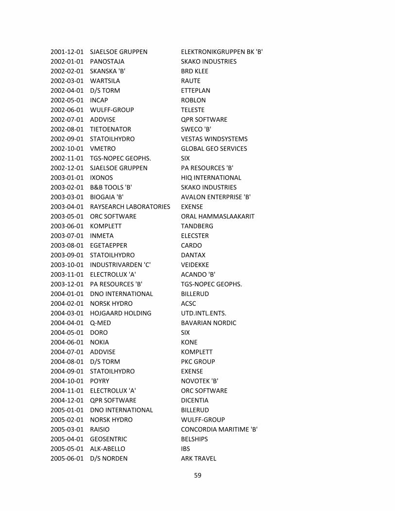
59

2001-12-01 SJAELSOE GRUPPEN ELEKTRONIKGRUPPEN BK 'B'

2002-01-01 PANOSTAJA SKAKO INDUSTRIES

2002-02-01 SKANSKA 'B' BRD KLEE

2002-03-01 WARTSILA RAUTE

2002-04-01 D/S TORM ETTEPLAN

2002-05-01 INCAP ROBLON

2002-06-01 WULFF-GROUP TELESTE

2002-07-01 ADDVISE QPR SOFTWARE

2002-08-01 TIETOENATOR SWECO 'B'

2002-09-01 STATOILHYDRO VESTAS WINDSYSTEMS

2002-10-01 VMETRO GLOBAL GEO SERVICES

2002-11-01 TGS-NOPEC GEOPHS. SIX

2002-12-01 SJAELSOE GRUPPEN PA RESOURCES 'B'

2003-01-01 IXONOS HIQ INTERNATIONAL

2003-02-01 B&B TOOLS 'B' SKAKO INDUSTRIES

2003-03-01 BIOGAIA 'B' AVALON ENTERPRISE 'B'

2003-04-01 RAYSEARCH LABORATORIES EXENSE

2003-05-01 ORC SOFTWARE ORAL HAMMASLAAKARIT

2003-06-01 KOMPLETT TANDBERG

2003-07-01 INMETA ELECSTER

2003-08-01 EGETAEPPER CARDO

2003-09-01 STATOILHYDRO DANTAX

2003-10-01 INDUSTRIVARDEN 'C' VEIDEKKE

2003-11-01 ELECTROLUX 'A' ACANDO 'B'

2003-12-01 PA RESOURCES 'B' TGS-NOPEC GEOPHS.

2004-01-01 DNO INTERNATIONAL BILLERUD

2004-02-01 NORSK HYDRO ACSC

2004-03-01 HOJGAARD HOLDING UTD.INTL.ENTS.

2004-04-01 Q-MED BAVARIAN NORDIC

2004-05-01 DORO SIX

2004-06-01 NOKIA KONE

2004-07-01 ADDVISE KOMPLETT

2004-08-01 D/S TORM PKC GROUP

2004-09-01 STATOILHYDRO EXENSE

2004-10-01 POYRY NOVOTEK 'B'

2004-11-01 ELECTROLUX 'A' ORC SOFTWARE

2004-12-01 QPR SOFTWARE DICENTIA

2005-01-01 DNO INTERNATIONAL BILLERUD

2005-02-01 NORSK HYDRO WULFF-GROUP

2005-03-01 RAISIO CONCORDIA MARITIME 'B'

2005-04-01 GEOSENTRIC BELSHIPS

2005-05-01 ALK-ABELLO IBS

2005-06-01 D/S NORDEN ARK TRAVEL

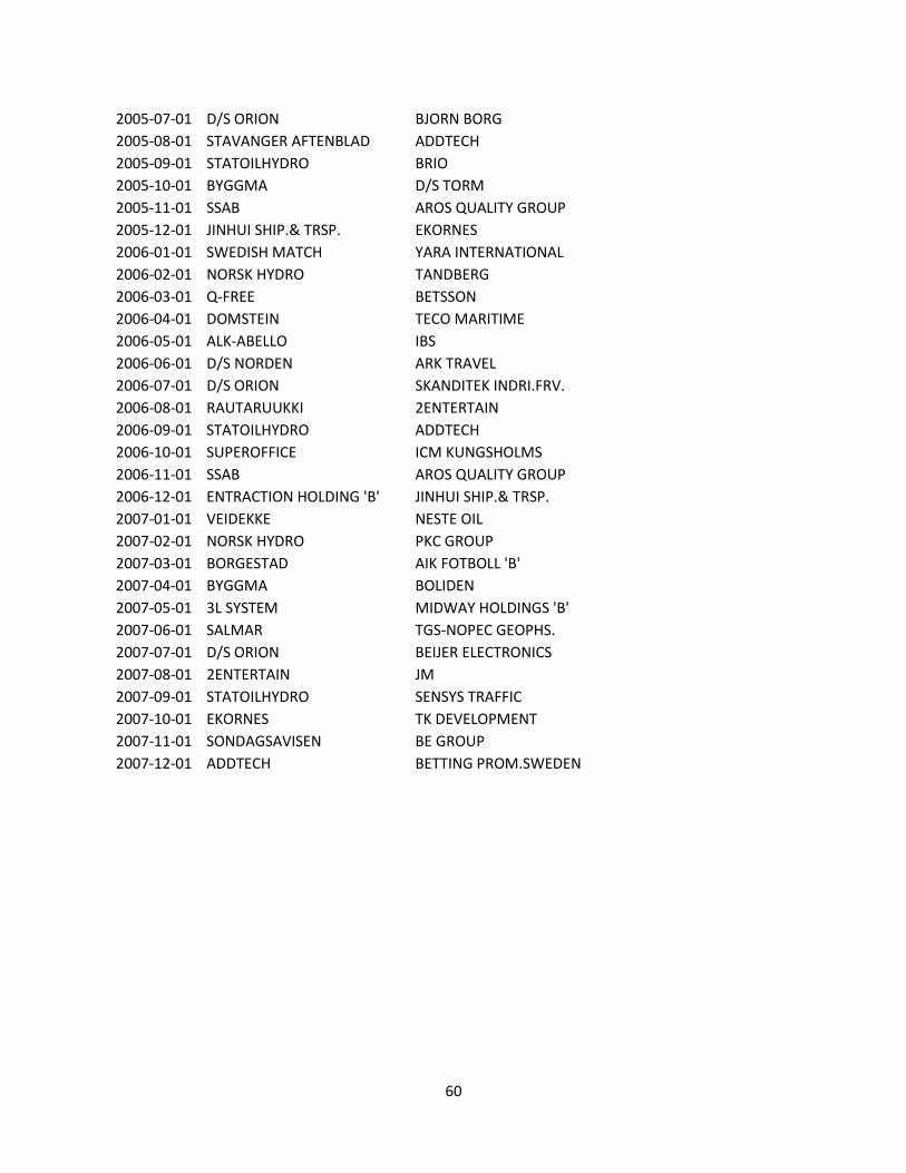
60

2005-07-01 D/S ORION BJORN BORG

2005-08-01 STAVANGER AFTENBLAD ADDTECH

2005-09-01 STATOILHYDRO BRIO

2005-10-01 BYGGMA D/S TORM

2005-11-01 SSAB AROS QUALITY GROUP

2005-12-01 JINHUI SHIP.& TRSP. EKORNES

2006-01-01 SWEDISH MATCH YARA INTERNATIONAL

2006-02-01 NORSK HYDRO TANDBERG

2006-03-01 Q-FREE BETSSON

2006-04-01 DOMSTEIN TECO MARITIME

2006-05-01 ALK-ABELLO IBS

2006-06-01 D/S NORDEN ARK TRAVEL

2006-07-01 D/S ORION SKANDITEK INDRI.FRV.

2006-08-01 RAUTARUUKKI 2ENTERTAIN

2006-09-01 STATOILHYDRO ADDTECH

2006-10-01 SUPEROFFICE ICM KUNGSHOLMS

2006-11-01 SSAB AROS QUALITY GROUP

2006-12-01 ENTRACTION HOLDING 'B' JINHUI SHIP.& TRSP.

2007-01-01 VEIDEKKE NESTE OIL

2007-02-01 NORSK HYDRO PKC GROUP

2007-03-01 BORGESTAD AIK FOTBOLL 'B'

2007-04-01 BYGGMA BOLIDEN

2007-05-01 3L SYSTEM MIDWAY HOLDINGS 'B'

2007-06-01 SALMAR TGS-NOPEC GEOPHS.

2007-07-01 D/S ORION BEIJER ELECTRONICS

2007-08-01 2ENTERTAIN JM

2007-09-01 STATOILHYDRO SENSYS TRAFFIC

2007-10-01 EKORNES TK DEVELOPMENT

2007-11-01 SONDAGSAVISEN BE GROUP

2007-12-01 ADDTECH BETTING PROM.SWEDEN

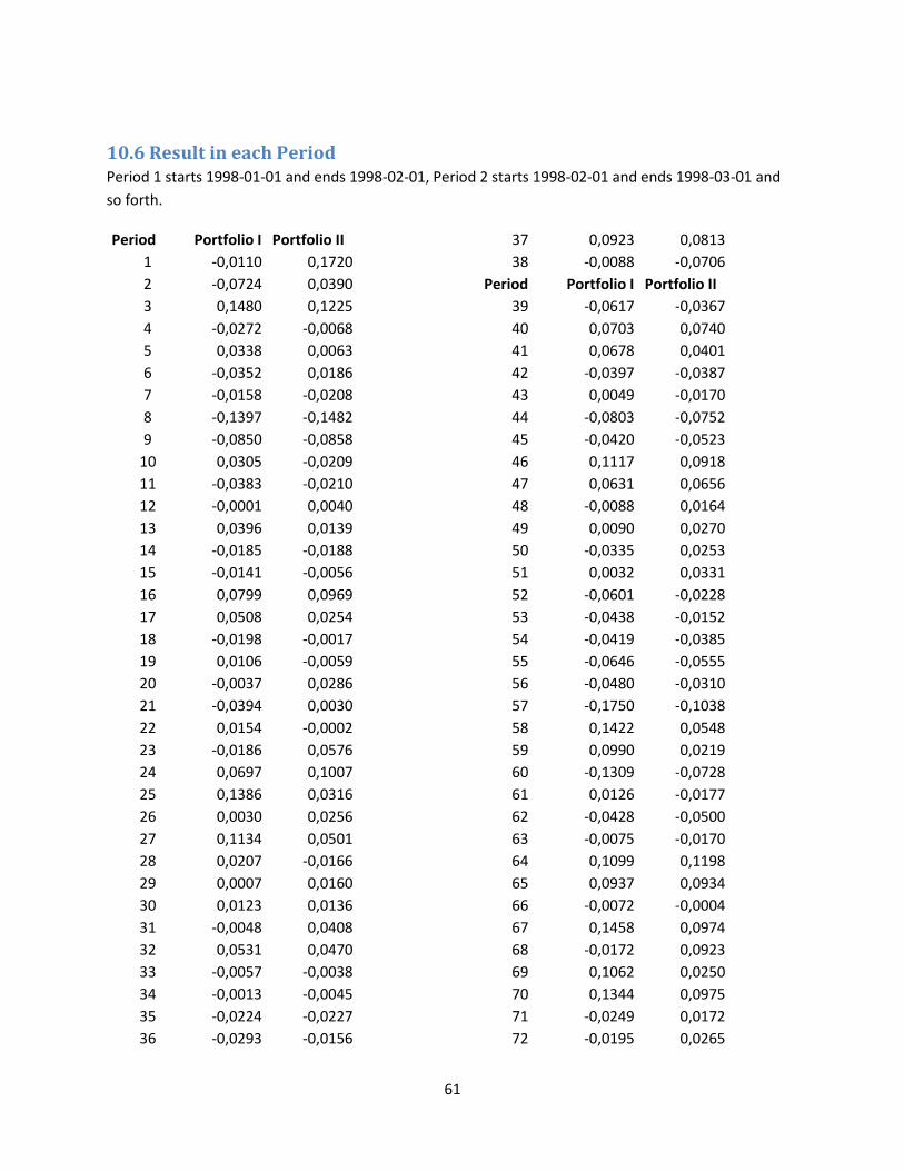
61

10.6 Result in each Period Period 1 starts 1998-01-01 and ends 1998-02-01, Period 2 starts 1998-02-01 and ends 1998-03-01 and

so forth.

Period Portfolio I Portfolio II

1 -0,0110 0,1720

2 -0,0724 0,0390

3 0,1480 0,1225

4 -0,0272 -0,0068

5 0,0338 0,0063

6 -0,0352 0,0186

7 -0,0158 -0,0208

8 -0,1397 -0,1482

9 -0,0850 -0,0858

10 0,0305 -0,0209

11 -0,0383 -0,0210

12 -0,0001 0,0040

13 0,0396 0,0139

14 -0,0185 -0,0188

15 -0,0141 -0,0056

16 0,0799 0,0969

17 0,0508 0,0254

18 -0,0198 -0,0017

19 0,0106 -0,0059

20 -0,0037 0,0286

21 -0,0394 0,0030

22 0,0154 -0,0002

23 -0,0186 0,0576

24 0,0697 0,1007

25 0,1386 0,0316

26 0,0030 0,0256

27 0,1134 0,0501

28 0,0207 -0,0166

29 0,0007 0,0160

30 0,0123 0,0136

31 -0,0048 0,0408

32 0,0531 0,0470

33 -0,0057 -0,0038

34 -0,0013 -0,0045

35 -0,0224 -0,0227

36 -0,0293 -0,0156

37 0,0923 0,0813

38 -0,0088 -0,0706


39 -0,0617 -0,0367

40 0,0703 0,0740

41 0,0678 0,0401

42 -0,0397 -0,0387

43 0,0049 -0,0170

44 -0,0803 -0,0752

45 -0,0420 -0,0523

46 0,1117 0,0918

47 0,0631 0,0656

48 -0,0088 0,0164

49 0,0090 0,0270

50 -0,0335 0,0253

51 0,0032 0,0331

52 -0,0601 -0,0228

53 -0,0438 -0,0152

54 -0,0419 -0,0385

55 -0,0646 -0,0555

56 -0,0480 -0,0310

57 -0,1750 -0,1038

58 0,1422 0,0548

59 0,0990 0,0219

60 -0,1309 -0,0728

61 0,0126 -0,0177

62 -0,0428 -0,0500

63 -0,0075 -0,0170

64 0,1099 0,1198

65 0,0937 0,0934

66 -0,0072 -0,0004

67 0,1458 0,0974

68 -0,0172 0,0923

69 0,1062 0,0250

70 0,1344 0,0975

71 -0,0249 0,0172

72 -0,0195 0,0265

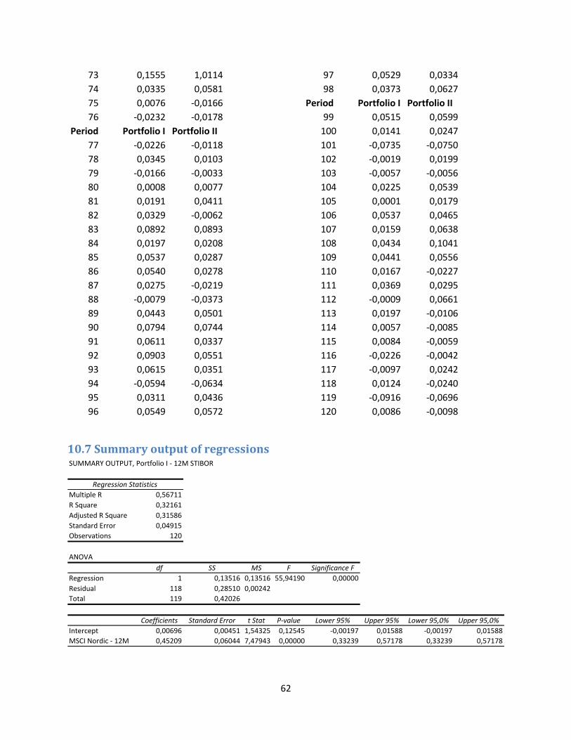
62

73 0,1555 1,0114

74 0,0335 0,0581

75 0,0076 -0,0166

76 -0,0232 -0,0178


77 -0,0226 -0,0118

78 0,0345 0,0103

79 -0,0166 -0,0033

80 0,0008 0,0077

81 0,0191 0,0411

82 0,0329 -0,0062

83 0,0892 0,0893

84 0,0197 0,0208

85 0,0537 0,0287

86 0,0540 0,0278

87 0,0275 -0,0219

88 -0,0079 -0,0373

89 0,0443 0,0501

90 0,0794 0,0744

91 0,0611 0,0337

92 0,0903 0,0551

93 0,0615 0,0351

94 -0,0594 -0,0634

95 0,0311 0,0436

96 0,0549 0,0572

97 0,0529 0,0334

98 0,0373 0,0627


99 0,0515 0,0599

100 0,0141 0,0247

101 -0,0735 -0,0750

102 -0,0019 0,0199

103 -0,0057 -0,0056

104 0,0225 0,0539

105 0,0001 0,0179

106 0,0537 0,0465

107 0,0159 0,0638

108 0,0434 0,1041

109 0,0441 0,0556

110 0,0167 -0,0227

111 0,0369 0,0295

112 -0,0009 0,0661

113 0,0197 -0,0106

114 0,0057 -0,0085

115 0,0084 -0,0059

116 -0,0226 -0,0042

117 -0,0097 0,0242

118 0,0124 -0,0240

119 -0,0916 -0,0696

120 0,0086 -0,0098

10.7 Summary output of regressions SUMMARY OUTPUT, Portfolio I - 12M STIBOR

Regression Statistics

Multiple R 0,56711

R Square 0,32161

Adjusted R Square 0,31586

Standard Error 0,04915

Observations 120

ANOVA

df SS MS F Significance F

Regression 1 0,13516 0,13516 55,94190 0,00000

Residual 118 0,28510 0,00242

Total 119 0,42026

Coefficients Standard Error t Stat P-value Lower 95% Upper 95% Lower 95,0% Upper 95,0%

Intercept 0,00696 0,00451 1,54325 0,12545 -0,00197 0,01588 -0,00197 0,01588

MSCI Nordic - 12M 0,45209 0,06044 7,47943 0,00000 0,33239 0,57178 0,33239 0,57178

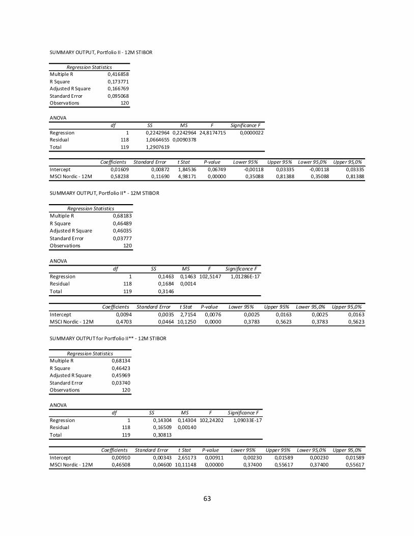
63

SUMMARY OUTPUT, Portfolio II - 12M STIBOR


Multiple R 0,416858

R Square 0,173771



Observations 120

ANOVA


Regression 1 0,2242964 0,2242964 24,8174715 0,0000022

Residual 118 1,0664655 0,0090378

Total 119 1,2907619


Intercept 0,01609 0,00872 1,84536 0,06749 -0,00118 0,03335 -0,00118 0,03335

MSCI Nordic - 12M 0,58238 0,11690 4,98171 0,00000 0,35088 0,81388 0,35088 0,81388

SUMMARY OUTPUT, Portfolio II* - 12M STIBOR


Multiple R 0,68183

R Square 0,46489



Observations 120

ANOVA


Regression 1 0,1463 0,1463 102,5147 1,01286E-17

Residual 118 0,1684 0,0014

Total 119 0,3146


Intercept 0,0094 0,0035 2,7154 0,0076 0,0025 0,0163 0,0025 0,0163

MSCI Nordic - 12M 0,4703 0,0464 10,1250 0,0000 0,3783 0,5623 0,3783 0,5623

SUMMARY OUTPUT for Portfolio II** - 12M STIBOR


Multiple R 0,68134

R Square 0,46423



Observations 120

ANOVA


Regression 1 0,14304 0,14304 102,24202 1,09033E-17

Residual 118 0,16509 0,00140

Total 119 0,30813


Intercept 0,00910 0,00343 2,65173 0,00911 0,00230 0,01589 0,00230 0,01589

MSCI Nordic - 12M 0,46508 0,04600 10,11148 0,00000 0,37400 0,55617 0,37400 0,55617

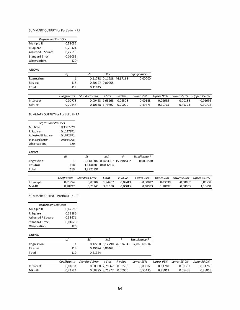
64

SUMMARY OUTPUT for Portfolio I - RF


Multiple R 0,53032

R Square 0,28124



Observations 120

ANOVA


Regression 1 0,11788 0,11788 46,17163 0,00000

Residual 118 0,30127 0,00255

Total 119 0,41915


Intercept 0,00778 0,00463 1,68168 0,09528 -0,00138 0,01695 -0,00138 0,01695

Mkt-RF 0,70244 0,10338 6,79497 0,00000 0,49773 0,90715 0,49773 0,90715

SUMMARY OUTPUT for Portfolio II - RF


Multiple R 0,3387729

R Square 0,1147671



Observations 120

ANOVA


Regression 1 0,1483387 0,1483387 15,2982492 0,0001538

Residual 118 1,1441808 0,0096964

Total 119 1,2925194


Intercept 0,01754 0,00902 1,94467 0,05419 -0,00032 0,03539 -0,00032 0,03539

Mkt-RF 0,78797 0,20146 3,91130 0,00015 0,38903 1,18692 0,38903 1,18692

SUMMARY OUTPUT, Portfolio II* - RF


Multiple R 0,62599

R Square 0,39186



Observations 120

ANOVA


Regression 1 0,12290 0,12290 76,03434 2,08577E-14

Residual 118 0,19074 0,00162

Total 119 0,31364


Intercept 0,01031 0,00368 2,79967 0,00598 0,00302 0,01760 0,00302 0,01760

Mkt-RF 0,71724 0,08225 8,71977 0,00000 0,55435 0,88013 0,55435 0,88013

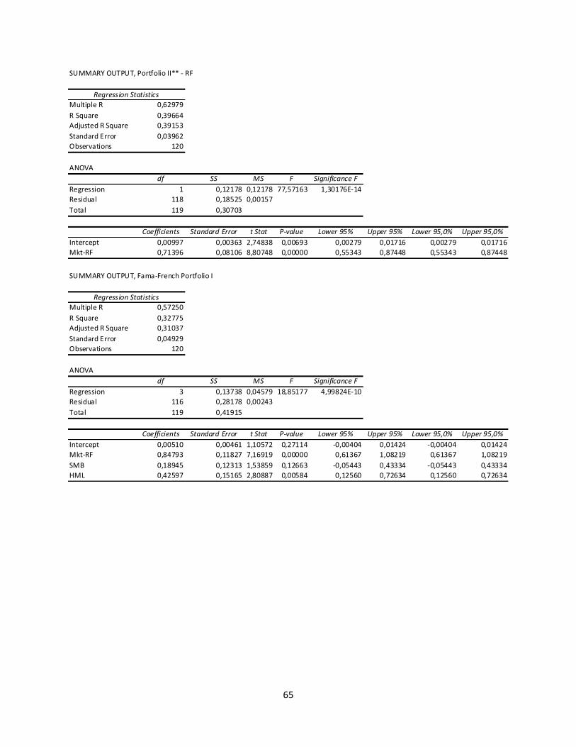
65

SUMMARY OUTPUT, Portfolio II** - RF


Multiple R 0,62979

R Square 0,39664



Observations 120

ANOVA


Regression 1 0,12178 0,12178 77,57163 1,30176E-14

Residual 118 0,18525 0,00157

Total 119 0,30703


Intercept 0,00997 0,00363 2,74838 0,00693 0,00279 0,01716 0,00279 0,01716

Mkt-RF 0,71396 0,08106 8,80748 0,00000 0,55343 0,87448 0,55343 0,87448

SUMMARY OUTPUT, Fama-French Portfolio I


Multiple R 0,57250

R Square 0,32775



Observations 120

ANOVA


Regression 3 0,13738 0,04579 18,85177 4,99824E-10

Residual 116 0,28178 0,00243

Total 119 0,41915


Intercept 0,00510 0,00461 1,10572 0,27114 -0,00404 0,01424 -0,00404 0,01424

Mkt-RF 0,84793 0,11827 7,16919 0,00000 0,61367 1,08219 0,61367 1,08219

SMB 0,18945 0,12313 1,53859 0,12663 -0,05443 0,43334 -0,05443 0,43334

HML 0,42597 0,15165 2,80887 0,00584 0,12560 0,72634 0,12560 0,72634

66

SUMMARY OUTPUT, Fama-French Portfolio II


Multiple R 0,38889

R Square 0,15124



Observations 120

ANOVA


Regression 3 0,19547 0,06516 6,88973 0,00026

Residual 116 1,09705 0,00946

Total 119 1,29252


Intercept 0,01346 0,00910 1,47878 0,14191 -0,00457 0,03149 -0,00457 0,03149

Mkt-RF 0,95463 0,23337 4,09058 0,00008 0,49241 1,41686 0,49241 1,41686

SMB 0,42353 0,24296 1,74321 0,08395 -0,05768 0,90475 -0,05768 0,90475

HML 0,60081 0,29923 2,00783 0,04698 0,00814 1,19348 0,00814 1,19348

SUMMARY OUTPUT, Fama-French Portfolio II*


Multiple R 0,66873

R Square 0,44721



Observations 120

ANOVA


Regression 3 0,14026 0,04675 31,28102 0,00000

Residual 116 0,17338 0,00149

Total 119 0,3136397


Intercept 0,00783 0,00362 2,16458 0,03247 0,00067 0,01500 0,00067 0,01500

Mkt-RF 0,81875 0,09278 8,82499 0,00000 0,63499 1,00250 0,63499 1,00250

SMB 0,25644 0,09659 2,65497 0,00905 0,06513 0,44774 0,06513 0,44774

HML 0,36510 0,11896 3,06917 0,00267 0,12949 0,60071 0,12949 0,60071

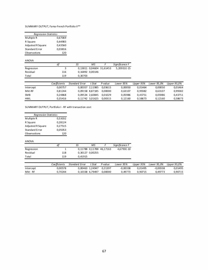
67

SUMMARY OUTPUT, Fama-French Portfolio II**


Multiple R 0,67069

R Square 0,44983



Observations 120

ANOVA


Regression 3 0,13811 0,04604 31,61453 5,20931E-15

Residual 116 0,16892 0,00146

Total 119 0,30703


Intercept 0,00757 0,00357 2,11985 0,03615 0,00050 0,01464 0,00050 0,01464

Mkt-RF 0,81244 0,09158 8,87185 0,00000 0,63107 0,99382 0,63107 0,99382

SMB 0,24868 0,09534 2,60845 0,01029 0,05986 0,43751 0,05986 0,43751

HML 0,35416 0,11742 3,01625 0,00315 0,12160 0,58673 0,12160 0,58673

SUMMARY OUTPUT, Portfolio I - RF with transaction cost


Multiple R 0,53032

R Square 0,28124



Observations 120

ANOVA


Regression 1 0,11788 0,11788 46,17163 4,6793E-10

Residual 118 0,30127 0,00255

Total 119 0,41915


Intercept 0,00578 0,00463 1,24947 0,21397 -0,00338 0,01495 -0,00338 0,01495

Mkt - RF 0,70244 0,10338 6,79497 0,00000 0,49773 0,90715 0,49773 0,90715

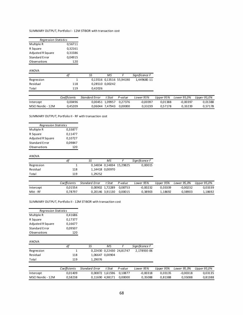
68

SUMMARY OUTPUT, Portfolio I - 12M STIBOR with transaction cost


Multiple R 0,56711

R Square 0,32161



Observations 120

ANOVA


Regression 1 0,13516 0,13516 55,94190 1,44968E-11

Residual 118 0,28510 0,00242

Total 119 0,42026


Intercept 0,00496 0,00451 1,09957 0,27376 -0,00397 0,01388 -0,00397 0,01388

MSCI Nordic - 12M 0,45209 0,06044 7,47943 0,00000 0,33239 0,57178 0,33239 0,57178

SUMMARY OUTPUT, Portfolio II - RF with transaction cost


Multiple R 0,33877

R Square 0,11477



Observations 120

ANOVA


Regression 1 0,14834 0,14834 15,29825 0,00015

Residual 118 1,14418 0,00970

Total 119 1,29252


Intercept 0,01554 0,00902 1,72289 0,08753 -0,00232 0,03339 -0,00232 0,03339

Mkt - RF 0,78797 0,20146 3,91130 0,00015 0,38903 1,18692 0,38903 1,18692

SUMMARY OUTPUT, Portfolio II - 12M STIBOR with transaction cost


Multiple R 0,41686

R Square 0,17377



Observations 120

ANOVA


Regression 1 0,22430 0,22430 24,81747 2,17893E-06

Residual 118 1,06647 0,00904

Total 119 1,29076


Intercept 0,01409 0,00872 1,61596 0,10877 -0,00318 0,03135 -0,00318 0,03135

MSCI Nordic - 12M 0,58238 0,11690 4,98171 0,00000 0,35088 0,81388 0,35088 0,81388

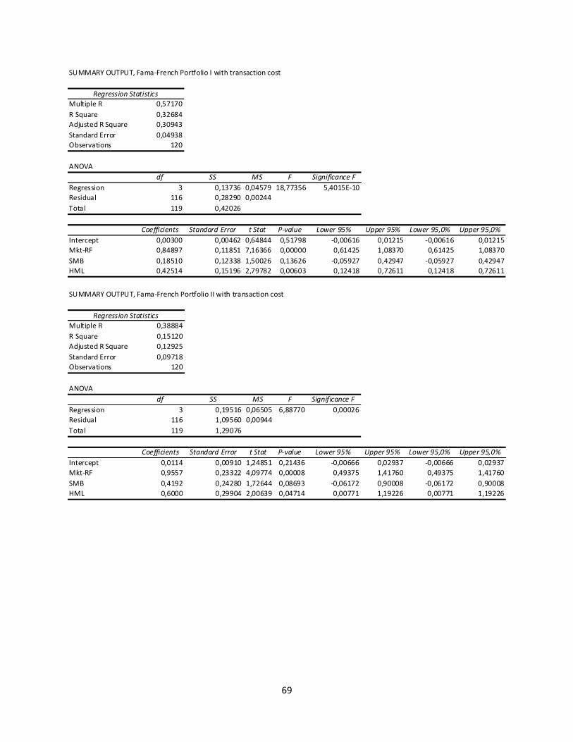
69

SUMMARY OUTPUT, Fama-French Portfolio I with transaction cost


Multiple R 0,57170

R Square 0,32684



Observations 120

ANOVA


Regression 3 0,13736 0,04579 18,77356 5,4015E-10

Residual 116 0,28290 0,00244

Total 119 0,42026


Intercept 0,00300 0,00462 0,64844 0,51798 -0,00616 0,01215 -0,00616 0,01215

Mkt-RF 0,84897 0,11851 7,16366 0,00000 0,61425 1,08370 0,61425 1,08370

SMB 0,18510 0,12338 1,50026 0,13626 -0,05927 0,42947 -0,05927 0,42947

HML 0,42514 0,15196 2,79782 0,00603 0,12418 0,72611 0,12418 0,72611

SUMMARY OUTPUT, Fama-French Portfolio II with transaction cost


Multiple R 0,38884

R Square 0,15120



Observations 120

ANOVA


Regression 3 0,19516 0,06505 6,88770 0,00026

Residual 116 1,09560 0,00944

Total 119 1,29076


Intercept 0,0114 0,00910 1,24851 0,21436 -0,00666 0,02937 -0,00666 0,02937

Mkt-RF 0,9557 0,23322 4,09774 0,00008 0,49375 1,41760 0,49375 1,41760

SMB 0,4192 0,24280 1,72644 0,08693 -0,06172 0,90008 -0,06172 0,90008

HML 0,6000 0,29904 2,00639 0,04714 0,00771 1,19226 0,00771 1,19226

Back testing “The Magic Formula” in the Nordic region

Documents

Transcript of Back testing “The Magic Formula” in the Nordic region