Delft University of Technology

Assessment of sectoral greenhouse gas emission reduction potentials for 2030

Blok, Kornelis; Afanador, Angélica; Van Der Hoorn, Irina; Berg, Tom; Edelenbosch, Oreane Y.; Van Vuuren,Detlef P.DOI10.3390/en13040943Publication date2020Document VersionFinal published versionPublished inEnergies

Citation (APA)Blok, K., Afanador, A., Van Der Hoorn, I., Berg, T., Edelenbosch, O. Y., & Van Vuuren, D. P. (2020).Assessment of sectoral greenhouse gas emission reduction potentials for 2030. Energies, 13(4),[en13040943]. https://doi.org/10.3390/en13040943

Important noteTo cite this publication, please use the final published version (if applicable).Please check the document version above.

CopyrightOther than for strictly personal use, it is not permitted to download, forward or distribute the text or part of it, without the consentof the author(s) and/or copyright holder(s), unless the work is under an open content license such as Creative Commons.

Takedown policyPlease contact us and provide details if you believe this document breaches copyrights.We will remove access to the work immediately and investigate your claim.

This work is downloaded from Delft University of Technology.For technical reasons the number of authors shown on this cover page is limited to a maximum of 10.

energies

Article

Assessment of Sectoral Greenhouse Gas EmissionReduction Potentials for 2030

Kornelis Blok 1,* , Angélica Afanador 2, Irina van der Hoorn 3, Tom Berg 3,Oreane Y. Edelenbosch 4,5 and Detlef P. van Vuuren 5,6

1 Faculty of Technology, Policy and Management, Delft University of Technology, Jaffalaan 5, 2628 BX Delft,The Netherlands

2 Navigant, a Guidehouse Company, Am Wassermann 36, 50829 Cologne, Germany;angelica.afanador@navigant.com

3 Navigant, a Guidehouse Company, Stadsplateau 15, 3521 AZ Utrecht, The Netherlands;irina.van.der.hoorn@navigant.com (I.v.d.H.); tom.berg@navigant.com (T.B.)

4 Present affiliation: Department of Management and Economics, Politecnico di Milan, I Via Lambruschini 4/B,20156 Milan, Italy; oreane.edelenbosch@polimi.it

5 PBL Netherlands Environmental Assessment Agency, Bezuidenhoutseweg 30, 2594 AV The Hague,The Netherlands; Detlef.vanVuuren@pbl.nl

6 Copernicus Institute of Sustainable Development, Utrecht University, Princetonlaan 8a, 3584 CB Utrecht,The Netherlands

* Correspondence: k.blok@tudelft.nl

Received: 20 January 2020; Accepted: 18 February 2020; Published: 20 February 2020�����������������

Abstract: The aim of this article is to provide an overview of greenhouse gas emission reductionpotentials for 2030 based on the assessment of detailed sectoral studies. The overview updatesa previous assessment that dates back more than ten years. We find a total emission reduction potentialof 30–36 GtCO2e compared to a current-policies baseline of 61 GtCO2e. The energy production andconversion sector is responsible for about one third of this potential and the agriculture, buildings,forestry, industry, and transport sectors all contribute substantially to the total potential. The potentialfor 2030 is enough to bridge the gap towards emissions pathways that are compatible with a maximumglobal temperature rise of 1.5–2 ◦C compared to preindustrial levels.

Keywords: emission reduction potential; emissions gap; energy production and conversion; sectoralanalysis; bottom-up analysis

1. Introduction

As part of the Paris Agreement process, an overwhelming majority of countries have submittedNationally Determined Contributions (NDCs) setting out their commitments with respect to thereduction of domestic greenhouse gas emissions. Most of these NDCs take 2030 as a target year.The total commitments falls short of being compatible with a long-term target of limiting globaltemperature rise to levels well below 2 ◦C compared to preindustrial levels [1–3]. In the coming year,the governments will be invited to put forward more ambitious commitments, but what is possible?An important question is what the total emission reduction potential is for the year 2030. This articleintends to show to what extent the portfolio of technologies and options that are available can providefor a sufficient reduction of global greenhouse gas emissions to be in line with the Paris Agreement.

Various methods exist to provide policy makers with information on climate change mitigationoptions. Scenarios that are supported by integrated assessment models (IAMs) provide information oncomprehensive strategies and account for the interactions between sectors. They can also provide insightinto the required level of reduction per sector to reach specific climate goals; see, e.g., Reference [4].

Energies 2020, 13, 943; doi:10.3390/en13040943 www.mdpi.com/journal/energies

Energies 2020, 13, 943 2 of 24

However, in general, the technical details of these assessments are relatively low, and in correspondencewith their scope and focus, most recent technological developments might be underrepresented [5].In contrast, studies that start with the (technology) options per sector can typically provide more detailin terms of emission reduction options—these are often referred to as bottom-up studies. They providea more disaggregated characterization and analysis but are generally less concerned with systemiceffects [6]. Such sectoral studies can provide, at a fairly detailed level, how much emission reductionis feasible within certain sectors or for specific emission categories. Ideally, these sectoral emissionreduction potentials present the mitigation options in a transparent way and provide a good indicationof the areas where climate mitigation action can be achieved. In the past, several studies have lookedat the strengths and weaknesses of these methods and at how they can be used together [7].

However, the most recent assessments of (bottom-up) sectoral emission reduction potentialsdate back more than eight years ago. These include the ones done for 2020 [8,9] and for 2030 bythe Intergovernmental Panel on Climate Change (IPCC) [10] and by McKinsey [11] (for a criticalassessment of the latter, see Reference [12]). More recent assessments were made by IPCC [13] and theInternational Energy Agency (IEA) [14], but both did not make a sector-by-sector assessment of the fullemission reduction potentials. In addition, several emission reduction potential assessments have beendone for specific regions, e.g., for the EU [15], for the US [16], and for 15 developing countries [17].Also, for specific sectors, assessments have been carried out, e.g., for the Chinese cement industry [18],for shipping [19], and for specific regional categories [20]. Therefore, the emission reduction potentialassessments that are available for 2030 either are partial or date back nearly a decade. Since then, climatepolicy ambitions have been formulated more clearly at the global level in the Paris Agreement as wellas at the national level. At the same time, greenhouse gas emissions (GHG) levels have continued toincrease and technology development continues [21], making the earlier emission reduction potentialassessments obsolete. There is thus an urgent need to fill this knowledge gap and to provide an updateon these studies. The aim of this article is to provide new sectoral GHG reduction potentials for 2030for all sectors at the global level. The focus will be on the socioeconomic potential.

In this article, we estimate the sectoral reduction potential by combining estimates of the impactof specific measures while accounting for their overlap. Based on a literature review, the potential ofavailable measures in all sectors contributing to GHG emissions, including the agriculture and forestrysector, the energy demand sectors, and the energy production and conversion sector, is estimated.This enables us to estimate the total emission reduction potential at the global level. We presenta comparison of this information with the emission reduction pathways generated through integratedassessment models (IAMs). While the IAMs have become more and more detailed over time and oftencontain many bottom-up elements, the outcomes between the two approaches can still differ [7] andcontrasting the two approaches provides additional insights.

After describing the methods in Section 2, the assessment of emission reduction potentials ona sector-by-sector basis is presented in Section 3. Section 4 provides an overview and discussion ofthe results, including a comparison with earlier estimates of the 2030 emission reduction potential,and compares the findings concerning the sectoral emission reduction potentials with the outcomes ofthe emission reductions calculated with integrated assessment models. The final section summarizesthe main conclusions.

2. Methods

2.1. Overall Method Used to Calculate Potential

Sectoral-based assessments can be used to assess different types of potential. The technicalpotential refers to the emission reduction that can be achieved by implementing the full set of availableoptions in a given future year. The socioeconomic potential is that part of the technical potentialwhich is economically attractive from a social cost perspective [22]. In this article, we specify thesocioeconomic potential as the collection of all emission reduction options that can be achieved at

Energies 2020, 13, 943 3 of 24

a marginal cost of no more than USD100/tCO2e, at current prices (not taking into account benefits otherthan saved energy costs). This level is similar to the cutoff level that was used in the 4th assessmentreport of the IPCC [10]. This was the previous global assessment of this type, and using the samecutoff level makes comparisons easier. It is also the carbon price level that is found to be necessary by2030 to achieve the ambitious reduction pathways that are more or less consistent with the objectivesformulated in the Paris Agreement [13,23].

The focus is on six key sectors: agriculture, buildings, energy production and conversion,forestry, industry, and transport. Waste-related options and carbon removal options not connected toa specific sector are discussed in the final subsection of Section 3. The following gases are included inthe analysis: carbon dioxide (CO2), methane (CH4), nitrous oxide (N2O), perfluorocarbons (PFCs),hydrofluorocarbons (HFCs), and sulphur hexafluoride (SF6). The assessment is done for the worldas a whole. We included all emission mitigation options as they are discussed in the literature andassessed, for example, in the sectoral chapters 7 through 11 of the last contribution of Working Group IIIto the IPCC (2014) assessment report. Some mitigation categories have not been included as no globalquantification is available yet (see the Discussion section). Our approach is in line with the approachfollowed in the Fourth Assessment Report of the IPCC [10]. First of all, for each sector, an overview ismade of (most recent) available literature on emission reduction potentials in 2030. Next, four elementsneed to be considered: (i) comparability: the studies need to have determined the potentials in ways thatlead to comparable results; (ii) coverage: all sectors and all major mitigation categories per sector needto be covered; (iii) baselines: the emission reduction potentials need to be referring to a coherent set ofbaselines; and (iv) aggregation: mitigation potentials influence each other, even cross-sectorally—thisneeds to be taken into account in the aggregation process [10]. There will be remaining uncertainties,but these are brought back to the levels that are indicated by the uncertainty ranges. We constrained thesample of abatement measures to those that could be realised through technologies that are available by2030. There are important uncertainties related to assumptions regarding technology development andimplementation rates, for example, how rapidly solar photovoltaic energy production can be scaled upand the rate at which buildings can be retrofitted. Most of the underlying analyses introduces somedegree of “realism” in the assessment and its respective assumptions. In general, it is assumed in thefollowing that the potentials can be achieved if countries around the globe are willing to set policiesthat enable the implementation of the available solutions.

We distinguish two types of potentials. First of all, the “basic potential” includes the categoriesfor which a long history of potential estimates is available. Next, some new categories are included forwhich only recently the first global estimates of emission reduction potentials were made. These areindicated as the “additional potential”. The potentials are calculated with reference to a current policyscenario. Such a scenario is needed to estimate future activity levels and to exclude measures thatare already implemented on the basis of such scenario. The main baseline scenario used here is theIEA World Energy Outlook [23]; for more details, see Section 2.2. In case the baseline emissionsfrom our literature sources deviated from the baseline emissions in WEO-2016, we corrected for thedifference, e.g., by proportionally scaling up or down the potential. In cases where potentials weregiven in terms of avoided fossil energy use, we calculated the emission reduction potentials based onaverage emission factors for 2030 from the World Energy Outlook. For the electricity sector, however,we use the average emission intensity of fossil-fuel-based power plants, as these are the emissionsthat are commonly avoided when emission reduction measures are taken [24]. The reasoning behindthis is that the plants with the highest marginal operating costs are those that are last in merit order.In general fossil-fuel-fired plants have the highest marginal costs; therefore, in case of more energyefficiency improvement or more renewables application, those plants are the first to reduce their output,which justifies our choice. Of course, there is some remaining uncertainty as the fuel mix avoided isnot known, but at a global level, this uncertainty will be limited. The average emission intensity forfossil-fuel-based power plants in 2030 is calculated to be 758 kg CO2/MWh in the baseline scenario.In some cases, a switch of energy carriers may occur, for example, from fuel to electricity (e.g., electric

Energies 2020, 13, 943 4 of 24

cars and heat pumps for buildings). In these cases, the potential was corrected for the additionalemissions associated with the additional electricity production, in line with the underlying sources.

For several sectors, there is potential overlap between the measures within the sector. In general,if in a sector two mitigation options are available that apply to the same emission category, the firstone measure is applied and then the emission reduction fraction of the second measure is applied tothe remaining emissions. For each sector, we discuss how we dealt with these overlaps at the endof the respective subsection in Section 3. The most important intersectoral overlap is between thepower sector and other sectors. Here, we took a (potentially too conservative) estimate based on themaximum potential that we found in a bottom-up analysis for the power sector.

For each emission category, we calculated the uncertainty of the size of the emission reductionpotentials. In some cases, the estimates we found in the literature were single-point potentials; in othercases, the estimates were given in ranges. To ensure consistency and to reflect the uncertainty ofthe size of the potentials, we applied a general ±25% uncertainty range to individual abatementcategories, which is in line with the uncertainty range that we find for those categories for whichan uncertainty range is given. For some measures, we applied a ±50% uncertainty range in orderto stay on the conservative side. We applied the latter to seven abatement measures out of 39 intotal: peatland degradation and peat fires, biochar, shifting dietary patterns, decreasing food loss andwaste, the various energy efficiency categories, and enhanced weathering measures. Most of these aremitigation options that have a relatively small track record in estimation of the size of the potential andwhich are therefore inherently more uncertain. We also had to include the energy efficiency measuresin this category, as we found out that these estimates showed some uncertainties, e.g., in some cases,they were based on extrapolation. Next, the estimates of energy efficiency potentials always have to bedetermined as the additional energy efficiency improvement compared to a significant autonomousdevelopment. This latter idea introduces additional uncertainty. For the calculation of the uncertaintyin sectoral aggregates and in the total, we applied the standard rules for error propagation [25].

2.2. Baseline Emissions

We use the Current Policies Scenario of the International Energy Agency’s World EnergyOutlook [23] as the baseline scenario. This scenario assumes no changes in policies from mid-2016onwards. In this article, we present for illustration purposes the degree of energy efficiency improvementfor all energy efficiency measures. We do this on the one hand compared to the baseline and on theother hand compared to the so-called frozen efficiency level. The calculate the latter, we assume that,in the Current Policies Scenario, the autonomous energy efficiency improvement rate is 1% per year,which is in line with historic developments [26].

For CO2 emissions from the calcination process in cement manufacturing, we used productiondata from Reference [14] and the emission factor for process emissions in cement [27].

Few recent baseline projections for the global forestry sector are published. These come witha considerable amount of uncertainty since forests are vulnerable to climate change, even underlow-warming scenarios [28]. We use emissions and absorption data from Reference [29].

Emissions from peatland degradation and peat fires are often not included in climate models.No baseline projections for peatland degradation are available. Taking into account trends in i)an increasing area of drained peatland, ii) a decreasing area of already drained peatland, and iii)a decreasing area of drained peatland, we assume they will remain at the current level [30]. Given theincreased awareness on the adverse effects of peat fires, we estimate that current emissions based onan extrapolation from Reference [31] will be halved [32].

For non-CO2 GHGs, we use baseline trajectories estimated by the United States EnvironmentalProtection Agency (USEPA) [33], unless more recent global baseline estimates were available. For energysector, methane emissions were taken from Reference [34] and was updated to become compatiblewith WEO-2016 [35]. Emissions originating from fluorinated gases (HFCs, PFCs, and SF6) were takenfrom Reference [36].

Energies 2020, 13, 943 5 of 24

For a detailed sectoral breakdown in the current policy projection, see Table 1. The total emissionsprojected for 2030 amount to 61.1 GtCO2e.

Table 1. Emissions by sector in the current policy scenario (GtCO2e): The emissions related to electricityproduction are also allocated to the end-use sectors, so these are listed twice in this table. These allocatedemissions are given in grey italics and not counted in the total.

Sector Category Gases 2030 Emissions(GtCO2e)

Sector Aggregates(GtCO2e)

Agriculture

Agricultural soils N2O 2.48

8.8

Enteric fermentation CH4 2.35

Manure CH4, N2O 0.38

Rice cultivation CH4, N2O 0.51

Other agricultural sources (includes burningof savannahs and from forest clearing andagricultural residues)

CH4, N2O 1.18

Peatland degradation CO2 1.6

Peat fires CO2, CH4 0.3

BuildingsFuel use (direct emissions) CO2 3.7

3.7Electricity use (indirect emissions) CO2 8.89

Energyproduction andconversion 1

Electricity production CO2 16.31

21.3Other energy conversion CO2 1.85

Natural gas and oil systems CH4 2.38

Coal mining CH4 0.73

Forestry

Deforestation CO2 3.44

3.5Afforestation and forest management CO2 −0.88

Other land-use change CO2 0.93

ManufacturingIndustry

Fuel use (direct emissions) CO2 7.31

12.7

Electricity use (indirect emissions) CO2 6.58

Process emissions for cement production CO2 2.3

Emissions from stationary and mobilecombustion CH4, N2O 0.77

Substitutes for ozone-depleting substances HFCs 1.6

Hydrochlorofluorocarbon-22 production HFC-23 0.2

Other industrial sources Allnon-CO2

0.5

TransportFuel use (direct emissions) CO2 9.42

9.4Electricity use (indirect emissions) CO2 0.28

Other

Other sectors electricity use (indirect emissions) CO2 0.56

1.7Landfilling of solid waste CH4 0.96

Other waste sources CH4, N2O 0.03

Wastewater CH4, N2O 0.71

Total 61.11 Includes emissions due to electricity use in end-use equipment.

3. Emission Reduction Potential for 2030 per Sector

3.1. Agriculture

In this subsection, we will first discuss options for the various agricultural production categories.Next, we will also discuss demand-side options.

Energies 2020, 13, 943 6 of 24

For croplands, Smith et al. [37] cite a 2030 mitigation and sequestration potential of 0.74 GtCO2e in2030 with 90% of the potential coming from CO2. The non-CO2 component is more or less in line withthe 0.04 GtCO2e from USEPA [38], presenting a range of options to reduce the emissions originatingfrom crop farming. The mitigation and sequestration can be established through a combination of 1)no-tillage and residue management, 2) agronomy, and 3) nutrient management, which are all assumedto be applied on one-third of global croplands. Recently, there has been discussion on no-tillagemeasures, for example, by Dimassi et al. [39], who argue that an increase in the soil carbon stock may bethe result of a redistribution of carbon between soil layers. However, this would not affect the potentialfrom Reference [37], since the area to which no-tillage measures are applied can be substituted withmeasures that have a more or less similar potential from the other cropland management categories,like agronomy and nutrient management. We therefore maintain the estimated potential of 0.74GtCO2e in 2030 for cropland management.

Grazing lands are typically managed less intensively than croplands, leaving significant potentialfor enhanced removals and emission reduction. Suggested grazing land measures by Smith et al. [37]include adjusting grazing intensity and allowing for more biomass growth; increasing land productivityby reducing nutrient deficiencies; using more precise nutrient additions, and thus, saving in fertilizer;managing fire (reducing frequency and fire intensity in fire-prone areas); and introducing species, e.g.,grass species with higher productivity from associated N inputs. They have estimated the impacts ofthese measures by combining emission reduction effects per area from a large database of experimentswith the area in various climate zones. Together, these measures have the potential to sequester 0.75GtCO2 in 2030.

Degraded peatlands drained for agricultural use disproportionally contribute to global GHGemissions from the land-use sectors [40]. When peatlands are drained, organic matter in soils startsoxidising and releases significant volumes of carbon emissions until drainage is reversed or all peatis lost [40]. Smith et al. [37] provides 2030 mitigation potentials for the restoration of cultivatedorganic (peaty) soils of 1.3 GtCO2e. Emissions from peatland fires can be nearly fully preventedcost-effectively, partly by the same measures and partly by additional fire control measures [41,42],leading to an emission reduction of 0.3 GtCO2e.

Based on a simulation of alternative rice management scenarios using varying managementtechniques, USEPA [38] estimates an emissions reduction potential of 0.18 GtCO2e in 2030. The optionsinclude measures such as adjusting the flooding regime, applying no-tillage, and using variousfertilizer alternatives.

Although current policy emissions from enteric fermentation and manure management make upa significant part of total agriculture emissions, the mitigation potential from livestock managementso far is limited. USEPA [38] estimates a global mitigation potential of 0.23 GtCO2e at costs belowUSD 100/tCO2 in 2030. The mitigation options with the highest cost-effective potentials are waste andmanure digesters, antimethanogens, intensive grazing, improved feed conversion, and propionateprecursors (animal feed additions that convert more of the produced hydrogen into propionate insteadof methane).

Based on a combination of intensive restoration projects on agricultural lands (15 million ha)and farmer-managed natural regeneration projects (135 million ha), the Global Commission on theEconomy and Climate estimates that an emission reduction of 1.1 GtCO2e can be achieved by 2030 [43].These estimates are scaled up from case-study results in China and Niger. We therefore applyan uncertainty range of 0.5–1.7 GtCO2e.

Recently, biochar has gained attention as a potential carbon removal option for agricultural lands,mainly cropland. Biochar is produced by heating biomass under anaerobic conditions, which underthe right conditions can enhance soil fertility and improve soil’s water retention properties whileenhancing the soil organic carbon content. Using a mix of dedicated crops, residues, manure, and otheragricultural inputs, Woolf et al. [44] estimate that a maximum of 1.8 GtCO2e per year can be mitigatedover the course of a century. Pratt and Moran [45] arrive at a similar potential. However, biochar

Energies 2020, 13, 943 7 of 24

production will ultimately be limited by the rate at which biomass can be extracted and pyrolyzedsustainably. Under their “maximum sustainable technical potential” scenario, Woolf et al. estimatethat, by 2030, a reduction of about 0.2 GtCO2e per year can be realized [44].

We now come to the emission reduction options related to the demand side of the food system.Efforts can be made to lower the carbon footprint of the average diet. Stehfest et al. [46] model theimpact of shifting food patterns to a diet recommended by the World Health Organization—whichsets recommendations on the consumption of animal products and fat—and compare this effect intwo different economic models: IMPACT from the International Food Policy Research Institute andLEITAP from the Global Trade Analysis Project. Both were coupled to the integrated assessment modelIMAGE. As a result of less agricultural demand, total GHG emissions decrease by 0.37 to 1.37 GtCO2ein 2030 in LEITAP and IMPACT, respectively [46].

Stehfest et al. [46] also studied the effect of reducing food waste, utilising the same methodsas described in the previous paragraph. Within the agricultural supply chain, significant losses canbe identified when considering factors such as harvesting inefficiency, bad harvesting conditions,deterioration during storage, or consumer behaviour. Estimates of total losses vary considerably,between 30–50% [47,48], and the effect of waste reduction is modelled as a 15 percent reduction inthe amount of food needed to meet similar nutrition levels, which requires a 45–75% reduction of thewasted amount of food. Modelled impacts on GHG emissions range from 0.97 GtCO2e to 2.0 GtCO2e.

Combining the potentials of all the measures discussed leads to a potential of 3 GtCO2e in 2030(uncertainty range 2.3–3.7 GtCO2e) if we exclude the “additional” measures like biochar, peat-relatedemission reductions, and the demand-side measures. The latter measures add up to a 3.7 GtCO2epotential (uncertainty range 2.6–4.8 GtCO2e) in 2030, after correction for overlap with the earliermeasures. Hence, the total emission reduction potential is 6.7 GtCO2e (uncertainty range 5.4–8 GtCO2e).

3.2. Buildings

We estimate that, for new buildings, between 0.68–0.85 GtCO2 could be avoided in 2030 based onthe method used by Reference [49]. This would require that all new buildings are near-zero energy incountries belonging to the Organisation for Economic Co-operation and Development (OECD) from2020 onwards and, in non-OECD countries, from 2020 to 2025 onwards (variation in start year leadingto the range in emission reductions). It is assumed that near-zero energy buildings have 90% loweremissions than the standard. This figure is consistent with Blok et al. [50], who estimated, based onan analysis of several studies, a potential of ambitious energy efficiency standards for new buildings of0.7–1.3 GtCO2 in 2030. It is also comparable with Reference [51], which reports a reduction potential of0.9 GtCO2 in 2030 for heating efficiency in new buildings. The improvement measures can include theapplication of heat pumps; the numbers presented here represent the net avoided emissions.

For the thermal retrofit of existing buildings, the estimated emission reduction potential is 0.53–0.93GtCO2 in 2030, using the same method as in Reference [49]. The lower range requires annual renovationrates of 3% in OECD and non-OECD countries from 2020 onwards with 75% direct emissions reductionper retrofit [52]. The higher range requires annual renovation rates of 5% in OECD countries and of 3%in non-OECD, in both cases, from 2020 onwards, with 90%direct emissions reduction per retrofit [52].These retrofit rates represent the highest reported in the literature. Typical historic retrofit rates are 1%per year; one of the highest numbers reported is for Germany, with a rate of just more than 2% [53].The reduction potential is consistent with Reference [51], which estimates a reduction potential of0.8 GtCO2 in existing buildings for 2030. Note that also, in these cases, the net emission mitigationpotential is reported, taking into account additional emissions in the power sector in the case of shiftsfrom fuels to electricity, e.g., through the use of heat pumps. The combined savings for new buildingsand building retrofits will lead to a reduction of the fuel use intensity of 33–60% in addition to what isachieved in the baseline (estimated to be 42–66% compared to 2015 frozen efficiency levels).

According to the International Renewable Energy Agency (IRENA) [54,55], heat from renewablesources can grow compared to the baseline by 5.4 EJ for solid, liquid, and gaseous biofuels and by 2.9

Energies 2020, 13, 943 8 of 24

EJ for solar energy. This equals an emission reduction potential of 0.39 GtCO2 in 2030 from biomassand of 0.21 GtCO2 for solar heat.

For electric appliances (excluding lighting) in households and the service sector, an assessmentof the potential is calculated based on Reference [56], leading to an emission reduction potentialof 3.3 GtCO2 in 2030. This is in line with the estimation of adopting the world’s best end-useequipment technology by the Collaborative Labeling and Appliance Standards Program (CLASP) [57].For energy-efficient lighting, a report by UNEP [58] estimates energy savings of 4.4 EJ, equivalent to 0.92GtCO2 in 2030. Molenbroek et al. [56] also reports emission reductions from lighting of 0.67 GtCO2 in2030. We will use this figure, which is slightly lower than the older estimate in Reference [57]. The totalsavings for appliances and lighting are equivalent to a reduction of the energy intensity in this categoryof 42% compared to the baseline (estimated to be 57% compared to 2015 frozen efficiency levels).Note that, in these numbers, only the impact of more efficient light sources is included and not othermeasures, such as more efficient luminaires. The same will apply to space cooling, for which betterarchitectural design can save more than what can be achieved by efficient cooling equipment alone.

Efficient behaviour of end-users is an option that can also reduce greenhouse gas emissions; see,e.g., Reference [59]. Providing advanced feedback to households facilitated by new technology likesmart meters and smart thermostats may save 5–15% in the EU or the US (see, e.g., References [60,61]).However, an estimate of the global emission mitigation potential is not available.

The total reduction potential for direct emissions from buildings is 1.9 GtCO2e (uncertainty range1.6–2.1 GtCO2e) in 2030 after correction for overlap between energy efficiency and renewable energymeasures. The reduction potential for indirect emissions is included in the potential for the energyproduction and conversion sector.

3.3. Energy Production and Conversion

A wide variety of emission reduction options exist in the power sector: a variety of renewableenergy sources, nuclear energy, and carbon capture and storage (CCS). Emission reductions from theoil and gas sector and from coal mining are also discussed in this section.

There is a wide range of estimates of solar photovoltaic (PV) potentials [62,63]. Solar powercapacity can reach 3725 GW in 2030 [64] compared to 708 GW in the reference scenario, which wouldprovide an emission reduction of 3.0 GtCO2 in 2030. The installed global solar capacity by the endof 2016 amounted to 303 GW [65]; reaching these potentials would require an annual growth ofinstalled capacity of 14–20% per year [64]. For comparison, the growth in the past decade amountedto 48% per year [65]. Some newer studies, however, provide higher potentials. A recent analysis byBreyer et al. [66] comes to a potential of 7100–9100 GW. This potential would require a growth ofthe installed solar PV capacity of 26–29% per year. For a more electrified energy system, Breyer etal. report a potential of 12,000 GW. Another study showed that, by scaling up the solar PV energystrategy of Germany to the whole world, solar PV, globally, could potentially increase in the range of3885–8722 GW by 2030 [67,68]. These potentials are also in range with those proposed by Haegel etal. [62]. Based on the large variety of numbers presented here and excluding the outliers, we come toa potential of 3–6 GtCO2 avoided through solar PV (total installed capacity 3700–8200 GW).

The installed global wind capacity by the end of 2016 was 487 GW [65]. Wind energy capacitycan grow to between 2110 and 3064 GW [64,69] compared to 940 GW in the reference scenario in 2030.This provides an emission reduction between 2.6–4.1 GtCO2; reaching these potentials would requirean annual growth of installed capacity of 11–15% per year. For comparison, the growth in the pastdecade amounted to 21% per year [65].

There are also other electricity production options that have potential to reduce emissions in thepower sector in 2030. Biomass has a potential of 0.85 GtCO2 and geothermal has a potential of 0.73GtCO2 compared to the baseline [64]. For hydro power and nuclear energy, the IEA [23] providesan indication for the potential of hydro and nuclear energy in its 450 scenario; with increases of 147

Energies 2020, 13, 943 9 of 24

GW and 154 GW compared to the baseline, the reduction potential is estimated as 0.32 and 0.87 GtCO2

in 2030, respectively.The total emission reduction potential for carbon capture and storage is estimated by IEA [14] as

2.03 GtCO2, which is slightly lower than the estimation by Mac Dowell and Fajardy [70] of 2.5 GtCO2

based on an earlier IEA study. This includes a reduction of 0.8 GtCO2 in 2030 for CO2 for enhancedoil recovery (EOR) and of 0.1 GtCO2 in 2030 for carbon capture and utilisation (CCU). Based on theallocation in Reference [14], 67% of the total potential will be allocated to the industry sector and 33%will be allocated to the power sector. The amount of carbon dioxide avoided is smaller than the amountof carbon dioxide captured because operating CCS consumes energy as well. This ratio is 70–90% [71].Therefore, we correct for the stored CO2 that is reported by applying a 20% discount. In the industrialsectors, a correction of 10% is applied since the CO2 in these sectors is often emitted at higher purity.Note that it is not certain that the entire CCS potential can be realised at costs below 100 USD/tCO2

(see Section 4.1).Bioenergy with carbon capture and storage (BECCS) has a reduction potential of 0.31 GtCO2 in

2030 [14]. Arasto et al. [72] estimate costs of 100–200 USD/tCO2, while McGlashan et al. [73] estimatethe average costs for BECCS to be 80–90 USD/tCO2 and Johnsen et al. [74] estimates that BECCS appliedon biofuel production in 2030 will cost €25–175/tCO2. Since there are studies with estimations underand above 100 USD/tCO2, the potential for BECCS will be allocated to the power sector category asan “additional” option.

We do not include the shift from coal to gas since natural gas declines in the World Energy Outlook450 scenario compared to the baseline [22]. However, within certain regions, the shift from coal togas can play a role in the reduction of emissions from the power sector; within the World EnergyOutlook 450 scenario, there is only a small increase visible in India (0.3 EJ) and South Africa (0.04EJ) [23]. Given the small size, this is not included in the potentials.

The total potential in the power sector is large—all numbers counted together make up about60–80% of the current policy scenario emissions in the power sector when summing up all individualpotentials, without considering overlap. Adding electricity savings from buildings and the industrysector have the potential to avoid the full current policy emissions in the power sector, bringing the totalto over 10%, which is obviously not possible unless BECCS is applied on a large scale. However, alreadylong before the 100% is reached, there will be increasing interactions between the different options,making the total potential smaller than the sum of the options. In the overall assessment, we assumethat total emissions in the power sector are not reduced by more than 57–65%, which are the largestfractions found in the literature [64,75]; this will lead to total emission reductions of 9.3–10.6 GtCO2.

Outside the power sector, methane emissions from the distribution of gas and the productionand transmission of oil and gas can be reduced by 1.78 GtCO2 in 2030 [35]. This is 75% of the baselineemissions from the oil and gas industry. These reductions can mainly be achieved by implementationof measures for the recovery and utilization of vented gas and the reduction of leakages.

Methane emissions from coal mining can be reduced by 0.41 GtCO2e in 2030, which is a reductionof 56% compared to the current policy scenario [35]. Measures implemented in this scenario includepre-mining degasification measures and the installation of ventilation air oxidisers.

Combining the potentials of all the electricity-related measures discussed in buildings and theindustry leads to a potential of 10.0 GtCO2e (range 9.3–10.6 GtCO2e) in 2030. BECCS could providean additional potential of 0.3 GtCO2e in 2030 (range 0.2–0.4 GtCO2e). Emission reductions from the oiland gas sector and from coal mining are 2.2 GtCO2e (range 1.7–2.6 GtCO2e).

3.4. Forestry

There are two main options in the forestry category: halting deforestation and restoration ofdegraded forest land. Emission reduction potentials from halting deforestation come with greatuncertainty. These uncertainties relate, for example, to the degree to which decreased deforestation

Energies 2020, 13, 943 10 of 24

leads to lowered degradation and associated carbon emissions and to which baseline is used [43].We assume a global potential in 2030 of 3 GtCO2e (based on Reference [4]).

Global commitments on the restoration of degraded forests aim to bring a total of 350 millionha of degraded and deforested land under restoration, such as commitments to the Bonn Challengeand the New York Declaration on Forests [76]. Reaching this target by 2030 would yield emissionreductions in the order of 1.6–3.4 GtCO2, with a central estimate of 2.3 GtCO2 in 2030 [77].

Combining the potentials of the measures discussed leads to a total contribution from the forestrysector of 5.3 GtCO2e (with an uncertainty range of 4.1–6.5 GtCO2e).

3.5. Manufacturing Industry

Two main options of industrial GHG emission reduction are energy efficiency improvement offuel and electricity use. There are also smaller sources of GHG emissions including “non-energy”use of fossil fuels (e.g., fossil fuels as feedstock for chemical processes) and emissions from industrialprocesses (for example, calcination in the cement process and several sources of non-CO2 GHGs).

For energy efficiency, the emission reduction potential for 2030 is estimated at 4.1 GtCO2 comparedto the current policy scenario. This estimate is based on data from ClimateWorks Foundation and theWorld Bank [78], scaled up from six major regions to the entire world and correcting for measuresother than energy efficiency. The analysis [78] covers all sectors. Both sector-specific technologiesand cross-cutting technologies (like heat recovery and energy-efficient motor systems) are included.The emission reduction means an additional reduction of the energy intensity of nearly 30% comparedto the current policy scenario (estimated to be 40% compared to 2015 frozen efficiency levels). This iscompatible with the estimate by Worrell and Carreon [79] (see also Reference [80]), who estimateda static potential of 27 ± 9%. Note that the potentials vary by sector and by region. For example, Worrelland Carreon estimate them to be 9 to 30%for iron and steel, 4 to 7% for primary aluminium, 20 to 25%for cement, 23 to 27% for petrochemicals, and 11 to 25% for ammonia production [79]. Based on theshare in current policy emissions, 2.2 GtCO2 emission reduction is allocated to direct emissions and 1.9GtCO2 is allocated to indirect emissions.

Renewable energy use in the form of solid, liquid, and gaseous biofuels; solar thermal energy;and geothermal can generate 9.7 EJ [54], which is an additional 7.8 EJ compared to the current policyscenario. This will save 0.5 GtCO2 in 2030.

Carbon capture and storage in the manufacturing industry has an emission reduction potentialof 1.22 GtCO2 in 2030; see the discussion of this option in the subsection on energy productionand conversion.

For non-CO2 greenhouse gases, the largest reduction is from HFCs, which can be reduced by 1.5GtCO2e in 2030 [36]. USEPA [38] estimates a reduction potential for other non-CO2 GHG emissions of0.2 GtCO2e in 2030, where 0.12 GtCO2e comes from nitric and adipic acid production and the rest isfrom reducing PFCs from primary aluminium production and SF6 from electric power systems andmagnesium production.

Measures to reduce the use of materials in society, like steel, cement, and plastics, can significantlyreduce emissions. This option is often called “dematerialization”, but no quantitative assessments areavailable for 2030. A study by Ecofys and Circle Economy [81] reports that circular economy measurescan reduce emissions in 2030 by 9.7 GtCO2. This number overlaps significantly with other measuresand is therefore not included in the overall add-up.

Based on the above, the reduction potential for the industry for the reduction of direct emissionsis 5.4 GtCO2e in 2030 (range 4.2–6.6 GtCO2e). No correction for overlap is needed, as many industrialplants are so large that energy efficiency measures can be combined with CCS or bioenergy, given therelatively small potentials of the latter. The reduction potential of indirect emissions is alreadyaccounted for in the potential for the energy supply sector.

Energies 2020, 13, 943 11 of 24

3.6. Transport

The emission reduction potential differs per mode of transport but is most significant forlight-duty vehicles and heavy-duty vehicles, with other contributions coming from shipping, aviation,and biofuels.

In the automobile sector, fuel efficiency measures could potentially reduce emissions by 0.88GtCO2 (high duty vehicles) and by 2.0 GtCO2 (light duty vehicles) by 2030 [82]. These numbers includemodal shifts, e.g., to public transport or nonmotorized transport. A shift to more electric vehicles is alsoincluded. The International Council on Clean Transportation (ICCT) [82] assumes that electric-drivevehicles will form a small but not insignificant share (up to 9%) of new-vehicle sales by 2030. This is inline with the estimations of IRENA [54] (10%). More recent sources, for example, Bloomberg NewEnergy Finance [83], consider higher market shares feasible (28% in 2030); no analysis is available on theimpact on global emissions in 2030, though. More use of nonmotorized transport, like cycling, can leadto significant emission reductions [84], but we have not included this as a separate option, as modalshifts are already included in the estimates of the ICCT. Note that substantial emission reductions dueto fuel economy standards for passenger cars are already included in the current policy scenario.

Aviation can reduce emissions by 0.32–0.42 GtCO2 in 2030 by using alternative fuels, improvedinfrastructure use, and technical improvements [82,85].

Several studies indicated an emission reduction for shipping [86–89], ranging from 0.39 to 0.99GtCO2. The studies contain several measures focused on fuel efficiency. The most recent study,from Bouman et al. [90], reports an emission reduction potential of 0.70 GtCO2 in 2030. The numbersfor aviation and shipping are in the same order as those in the study from New Climate Economy [91],which shows a reduction potential between 0.60 and 0.90 GtCO2 per year.

Another measure that is relevant for the transport sector is the application of biofuels. ICCT [82]provides no potential for biofuels due to the high uncertainty. IRENA [54] does provide an estimatefor biofuels to cover 10% of the sector’s total fuel use in 2030. Taking into account that greenhouse gasemissions from biofuels are 70–90% lower than those of conventional fuels [92], an emission reductionpotential of 0.63 to 0.81 GtCO2e in 2030 can be calculated.

Based on the above, the total emission reduction potential for the transport sector is 4.7 GtCO2ein 2030 (with an uncertainty of 4.1–5.3 GtCO2e). No overlap correction is needed, as biofuels canbe used as drop-in fuels. The energy efficiency measures alone will lead to a total sector energyintensity reduction of 42% compared to the baseline (estimated to be 54% compared to 2015 frozenefficiency levels).

3.7. Other

Some options for emission reduction are difficult to allocate to one of the sectors assessed in theprevious sections. This may be because it is still unknown in which sector it can best be implementedor because the option can be applied to multiple sectors. Some promising mitigation measures aredescribed below.

Methane constitutes some 90% of GHG emissions from the waste sector. An emission reductionoption is landfill gas recovery and utilization. USEPA [38] estimates that landfill gas recovery canreduce emissions by 0.4 GtCO2e in 2030, which is 42% of the emissions in the current policy scenario.

Enhanced weathering measures aim to draw carbon from the atmosphere via, among others,the natural chemical weathering process of silicates. Biogeochemical activity in soils naturallyaccelerates the weathering of rock and thereby leaches out calcium and magnesium, which then reactswith dissolved CO2 (HCO3

- and CO32-) [93]. First global estimates, assuming use of wastes from the

cement, iron, and steel and from the power industry, arrive at 0.73–1.22 GtCO2e [94].Direct capture of atmospheric CO2 from air is not included as the costs seem to be larger than

USD100/tCO2e [95].

Energies 2020, 13, 943 12 of 24

4. Total Emission Reduction Potentials

4.1. Total Emission Reduction Potential

An overview of the estimated total emission reduction potentials in 2030 assessed in the previoussection is provided in Table 2. The table shows that emission reduction categories have a longer historyof assessment, which we indicate as the “basic potential”, leading to a total emission reduction potentialin 2030 of 33 GtCO2e (uncertainty range 30–36 GtCO2e). If we consider, in addition, that options forwhich estimates of emission reduction potentials are relatively new and the feasibility of realising thesein 2030 is more uncertain (the “additional potential”), we get to a total potential of 38 GtCO2e (range35–41 GtCO2e). A sectoral breakdown is presented in Figure 1.

Energies 2020, 13, x FOR PEER REVIEW 12 of 25

Methane constitutes some 90% of GHG emissions from the waste sector. An emission reduction

option is landfill gas recovery and utilization. USEPA [38] estimates that landfill gas recovery can

reduce emissions by 0.4 GtCO2e in 2030, which is 42% of the emissions in the current policy scenario.

Enhanced weathering measures aim to draw carbon from the atmosphere via, among others, the

natural chemical weathering process of silicates. Biogeochemical activity in soils naturally accelerates

the weathering of rock and thereby leaches out calcium and magnesium, which then reacts with

dissolved CO2 (HCO3- and CO32-) [93]. First global estimates, assuming use of wastes from the cement,

iron, and steel and from the power industry, arrive at 0.73–1.22 GtCO2e [94].

Direct capture of atmospheric CO2 from air is not included as the costs seem to be larger than

USD100/tCO2e [95].

4. Total Emission Reduction Potentials

4.1. Total Emission Reduction Potential

An overview of the estimated total emission reduction potentials in 2030 assessed in the previous

section is provided in Table 2. The table shows that emission reduction categories have a longer

history of assessment, which we indicate as the “basic potential”, leading to a total emission reduction

potential in 2030 of 33 GtCO2e (uncertainty range 30–36 GtCO2e). If we consider, in addition, that

options for which estimates of emission reduction potentials are relatively new and the feasibility of

realising these in 2030 is more uncertain (the “additional potential”), we get to a total potential of 38

GtCO2e (range 35–41 GtCO2e). A sectoral breakdown is presented in Figure 1.

Figure 1. Sectoral emission reduction potentials at the global level compared to the total emissions

gap in 2030: Note that electricity efficiency options are included in the sector energy production and

conversion and not in the end-use sectors buildings and manufacturing industry. The total potential

is compared with the emission gap (see text for definition) [96].

According to the 2017 emissions gap report [96], the difference in 2030 between emissions under

the current policy scenario and the emission levels consistent with a likely chance of staying below 2

°C (>66% probability) and a medium chance of staying below 1.5 °C (50–66% probability) are

respectively 17 and 22.5 GtCO2e. Importantly, even if only the basic emission reduction potential for

2030 is considered, the estimated total potential listed in this report is more than sufficient to bridge

the emissions gap in 2030 for 2 °C and 1.5 °C.

0 5 10 15 20 25 30 35 40 45

Emission Gap

Total emission reduction

Other

Transport

Manufacturing Industry

Forestry

Energy production and conversion

Buildings

Agriculture

Emission reduction potential (Gt CO2e)

Emission Gap Basic potential Basic and Additional potential

Figure 1. Sectoral emission reduction potentials at the global level compared to the total emissionsgap in 2030: Note that electricity efficiency options are included in the sector energy production andconversion and not in the end-use sectors buildings and manufacturing industry. The total potential iscompared with the emission gap (see text for definition) [96].

According to the 2017 emissions gap report [96], the difference in 2030 between emissions underthe current policy scenario and the emission levels consistent with a likely chance of staying below 2 ◦C(>66% probability) and a medium chance of staying below 1.5 ◦C (50–66% probability) are respectively17 and 22.5 GtCO2e. Importantly, even if only the basic emission reduction potential for 2030 isconsidered, the estimated total potential listed in this report is more than sufficient to bridge theemissions gap in 2030 for 2 ◦C and 1.5 ◦C.

Energies 2020, 13, 943 13 of 24

Table 2. Overview of emission reduction potentials: Although for many emission reduction categoriesa single point estimate is given, there are always uncertainties, assumed to be ±25%. For the categoriesof peatland degradation and peat fires, biochar, and the various energy efficiency measures, the potentialin 2030 is more uncertain. Therefore, a higher uncertainty range of 50% is applied for these categories.In the final column, the categories are aggregated to the sectoral level (see discussion in the text).The numbers in the third column are not corrected for overlap between measures. The numbers in thefinal column are corrected for overlap, and this is also reflected in the total potential. Therefore, the totalis smaller than the sum of the individual potentials in the third column. The aggregate potentials forindirect emission reductions in buildings and industry are reflected in the electricity sector potential.

Sector Category Emission ReductionPotential in 2030 (GtCO2e) Category Sectoral Aggregate

Potential (GtCO2e)

Agriculture

Cropland management 0.74

Basic 3 (2.3–3.7)

Rice management 0.18

Livestock management 0.23

Grazing land management 0.75

Restoration of degraded agricultural land 0.5–1.7

Peatland degradation and peat fires 1.6

Additional 3.7 (2.6–4.8)Biochar 0.2

Shifting dietary patterns 0.37–1.37

Decreasing food loss and waste 0.97–2.0

Buildings

New buildings 0.68–0.85

Basic 1.9 (1.6–2.1)Existing buildings 0.52–0.93

Renewable heat—bioenergy 0.39

Renewable heat—solar energy 0.21

Lighting 0.67 Basic (indirectemissions)

See energy productionand conversionAppliances 3.3

Energyproduction and

conversion

Solar energy 3–6

Basic 10.0 (9.3–10.6)

Wind energy 2.6–4.1

Hydropower 0.32

Nuclear energy 0.87

Bioenergy 0.85

Geothermal 0.73

Carbon capture and storage 0.53

Bio-energy with carbon capture and storage 0.31 Additional 0.3 (0.2–0.4)

Methane from coal 0.41Basic 2.2 (1.7–2.6)

Methane from oil and gas 1.78

ForestryRestoration of degraded forest 1.6–3.4

Basic 5.3 (4.1–6.5)Reducing deforestation 3

ManufacturingIndustry

Energy efficiency—indirect 1.9 Basic (indirectemissions)

See energy productionand conversion

Energy efficiency—direct 2.2

Basic 5.4 (4.2–6.6)Renewable heat 0.5

Non-CO2 greenhouse gases 1.5

CCS 1.22

Transport

Heavy duty vehicles (efficiency, modal shift) 0.88

Basic 4.7 (4.1–5.3)

Light duty vehicles (efficiency, modal shift,electric vehicles) 2.0

Shipping efficiency 0.7

Aviation efficiency 0.32–0.42

Biofuels 0.63–0.81

OtherLandfill gas recovery 0.4 Basic 0.4 (0.3–0.5)

Enhanced weathering measures 0.73–1.22 Additional 1 (0.7–1.2)

Total basic emission reduction potential 33 (30–36)

Total emissions reduction potential including additional measures 38 (35–41)

Energies 2020, 13, 943 14 of 24

4.2. Discussion on Sectoral Emission Reduction Potentials

The sectoral assessment of emission reduction options relies on a variety of secondary sources,including both peer-reviewed and grey literature. Especially for the grey literature, we have carefullyexamined the sources that we used for quality and completeness. Use of grey literature is not necessarilya drawback: it can bring in expertise from outside academia and, sometimes, is more up to date.Nevertheless, there are still options for which limited information is available, e.g., the global mitigationimpact of circular economy options and changes in end-user behavior, so these are missing from theoverall analysis. Also, the potential impact of the introduction of new intermediate energy carriers,like hydrogen produced with electricity from renewable sources, is still insufficiently investigated.

Although the available studies prevent an explicit, economic assessment of all emission reductionoptions, there is a relatively high degree of confidence that all options included in Table 2 have costsbelow USD100 per tCO2e avoided. In many cases, this is explicitly mentioned in the source documents(referred to Section 3); in the remaining cases, this is supported by other sources [97,98]. For some,however, it is not clear whether the costs will fall below USD100/tCO2e. For example, some electricitysources may show costs above USD100/tCO2e in specific cases, as there are large variations in costs [98].However, given that there are abundant options in the electricity sector, leaving out these options willnot affect the total potential.

Energy efficiency options are spread across the sectors (including the sector energy productionand conversion; electricity efficiency options are included there). They make up a substantial partof the emission mitigation potential: about 13 GtCO2e. Nevertheless, this is also the area for whichcalculations of the global potential are relatively rare and better analysis is needed to get to more precisepotential estimates. There are indications that the potential might be higher than what is presented inthis assessment; see, for example, Reference [99]. One area that deserves specific mention is that ofelectric vehicles, where potentials currently are estimated to be higher than what we derived from ourprimary source. Another area that was not at all included in our analysis is material efficiency andother circular-economy-related options because of the lack of global analysis (see Section 3.5). The highpotential of reducing emissions by demand-side measures is also confirmed by Grübler et al. [100],leading to a level of final energy use in 2050 of 245 EJ (for comparison, in 2014, global final energyuse was approx. 400 EJ [23]). Our results also indicate that there is a potential for final energy use toalready decline in 2030, compared to current levels.

The 30–36 GtCO2e range found in this article is at the high end of the range of 15.8–31.1 GtCO2efound in the Fourth Assessment Report of the IPCC [10], even if we exclude the additional potential.Note that the IPCC report starts from a 7% lower baseline. A detailed comparison can be found inTable 3. In the current study, we find higher potentials for energy production and conversion (especiallyfor solar and wind energy), the forestry sector (higher potentials for reforestation), the industry sector(higher potentials for electricity efficiency), and the transport sector (higher potential for fuel efficiencyin all transportation modes). In most of these cases, the higher potential estimates that we find nowmay probably be related to a favourable development of the technology (e.g., much lower costs forsolar PV) or further exploration of the options. The potential estimate of 38 GtCO2e that was reportedby McKinsey [11] is in the high end of our range, but their baseline emissions are also not currentpolicies but rather business-as-usual and 15% higher; note that McKinsey included some options thatwe did not include, e.g., recycling. Our total results for agriculture and forestry of about 11 GtCO2efor the agriculture and forestry sectors compare well with the 11.3 GtCO2e found in the recent studyby Griscom et al. [101] for “natural climate solutions” (although they did not include demand-sidemeasures like dietary changes and prevention of food waste). For a comparison with the results ofintegrated assessment models, see Section 4.3.

Note that we counted all potentials together on the basis of global warming potentials (GWPs)with a time horizon of 100 years. This approach is the only suitable one if potentials for one specificyear are given. Nevertheless, it has its limitations, given that the reduction of relatively short-lived

Energies 2020, 13, 943 15 of 24

substances (like methane) will have a higher short-term impact than a similar CO2-equivalent emissionreduction impact of long-lived substances (like N2O).

Table 3. Comparison of our results to those of the Fourth Assessment Report of the IntergovernmentalPanel on Climate Change (IPCC) (in GtCO2e): Note that, in this table, the emission reductions due toelectricity savings in buildings and industry in this table are counted with the energy production andconversion sector, whereas in the Summary for Policy Makers of the IPCC report, they are countedwith the buildings and industry sector. Here, the respective emission reductions from the IPCC reportare reallocated to the energy production and conversion sector.

IPCC (2007) This Study Basic Potential(in Parenthesis Additional Potential)

Agriculture 2.3–6.4 2.3–3.7 (2.6–4.8)Buildings 2.3–2.9 1.6–2.1Energy production and conversion 6.2–9.3 11.4–13.0 (0.2–0.4)Forestry 1.3–4.2 4.1–6.5Manufacturing Industry 2.3–4.9 4.2–6.6Transport 1.6–2.5 4.1–5.3Waste 0.4–1.0 0.3–0.5

An important question is what the efforts and costs are of realising these emission reductions.Although it is beyond the scope of the current article to answer this question in full, a number ofobservations can be made. It is remarkable that a large part of the potential consists of just six relativelyhomogeneous categories, that is, solar and wind energy, efficient appliances, efficient passenger cars,afforestation, and stopping deforestation; they sum up to a potential of 18.5 GtCO2e in 2030 (range:15–22 GtCO2e), making up more than half of the basic potential. Equally important, all these measurescan be realised at modest or in some cases even net-negative costs and are predominantly achievablethrough proven policies. Solar PV and wind energy: Many countries around the world have targetsfor renewable energy and have policies in place to stimulate the adoption. The most dominant policyinstruments are feed-in tariffs or feed-in premiums, which have been implemented in 75 countries and29 states or provinces in the world, providing long-term power purchase agreements with a specifiedprice or premium price per kWh for a renewable energy technology [65]. An instrument with increasingpopularity is competitive bidding or auctioning, especially for large-scale developments, where therenewable energy market is mature and governments have already achieved a degree of successwith renewable energy installation through feed-in tariffs [65]. Costs of electricity from solar andwind electricity have already declined to levels comparable with fossil-fuel-based electricity [98],and auctions have accelerated this trend [102]. Continuation of feed-in policies and/or a shift to auctionsare a straightforward and cheap approach to rapid decarbonisation of the power sector. Energy-efficientappliances and cars: To stimulate the uptake of efficient appliances, the combination of labelling andminimum energy performance standards are the dominant policies. Over 60 countries have adopted orpledged to adopt policies to shift to more energy-efficient lighting [58]. Under the united for efficiency(U4E) public-private-partnership, UN Environment is supporting developing countries and emergingeconomies to move their markets to energy-efficient appliances and equipment [96]. In terms ofperformance standards for cars, countries have opted to implement fuel economy standards in milesper gallon or CO2 emission standards in gCO2 per km; these standards exist in Brazil, the EU, India,Japan, Mexico, and the USA [103]. Typically, energy efficiency standards are implemented in sucha way that lifecycle costs are minimized, hence leading to net-negative costs for the consumer. Similarpolicies are in place for new building construction [104]. Further continuation of these policies, scalingthem up to more countries while raising ambitions, is a way forward to limit the growth of energy useand hence to reduce emissions. Stopping deforestation and restoration of degraded forests: There areseveral examples of policies successfully stopping deforestation, the most large-scale being the Brazilian“Action Plan for Prevention and Control of Deforestation in the Amazon”, consisting of (1) territorial and

Energies 2020, 13, 943 16 of 24

land-use planning, (2) environmental control and monitoring, and (3) fostering sustainable productionactivities. The programme led to a reduction of the deforestation rate by over 80%. Costs are found tobe on average USD13/tCO2e [67,68]. For reforestation of degraded forests, the scale of operations is notthat size, but promising examples are available for China [105], Costa Rica [67,68], and the Republic ofKorea [106]. Costs are comparable with the costs of stopping deforestation.

4.3. Comparison of the Sectoral Results with Results from Integrated Assessment Models

The results of the bottom-up sector-by-sector assessment can be compared with the sectoralemissions as reported by a range of state-of-the-art integrated assessment models (IAMs). This is usefulbecause IAMs provide information on how a given climate target can be achieved in a “least-cost” waythrough a full cost comparison across all sectors and by taking into account the interactions between thedifferent reduction options and the interactions with the wider economy. Since the scenarios we discusshere stay within the 2 ◦C and 1.5 ◦C targets, they also bridge the gap between current policy emissionsin 2030 and the emissions in line with the 2 ◦C and 1.5 ◦C targets. Hence, the package of mitigationmeasures identified in the scenarios can be viewed as successful examples of how to close the gap.For the comparison, we use the baseline of the Shared Socioeconomic Pathways (SSP), a new scenarioframework facilitating the integrated analysis of future climate policy and impacts [107]. The SSP2scenario is the “middle-of-the-road” scenario of the Shared Socioeconomic Pathways. Six IAMs havebeen used to quantify the SSP scenarios, namely AIM/CGE, GCAM, IMAGE, MESSAGE-GLOBIOM,REMIND, and WITCH. AIM/CGE, REMIND, and WITCH are general equilibrium models usingintertemporal optimization solution algorithms. The other three models use a recursive dynamicapproach, with for GCAM a partial equilibrium framework, and for IMAGE and MESSAGE-GLOBIOM,a hybrid form [107]. Subsequently, we compare the derived mitigation scenarios aiming for a likely(>66%) probability of staying below 2 ◦C, with bottom-up assessment of the mitigation potential.It should be noted that the SSP2 baseline scenarios range from 62–69 GtCO2e, which is higher thanthe baseline emissions used in the sectoral assessment, i.e., 61.1 GtCO2e (Table 1). The reason is thatSSP2 shows emission development in the absence of climate policies, whereas the baseline of thesector-by-sector analysis is a current-policies scenario. Estimates of current policy scenarios in IAMmodels (e.g., Reference [108]) show a similar emission range as included in Table 1.

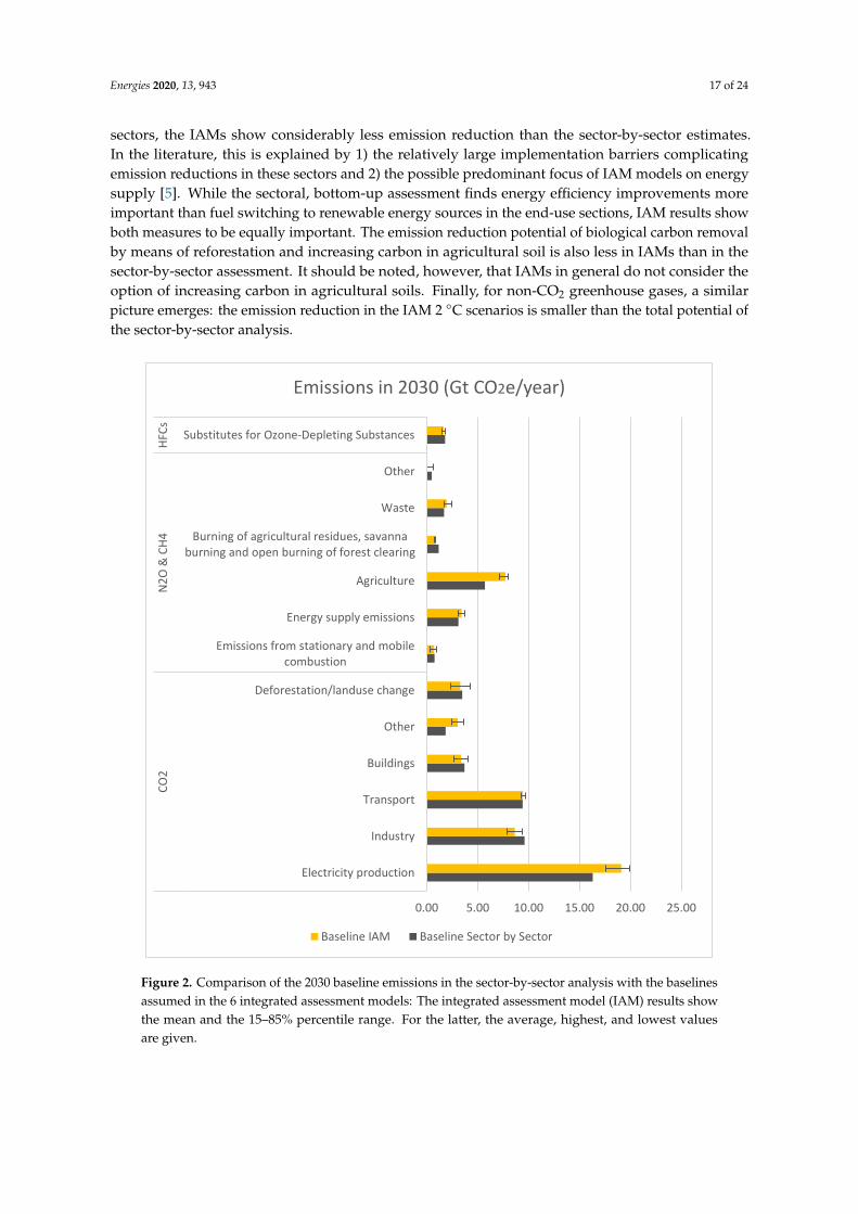
At the sector level, the projections from integrated assessment models show that baselineemissions can grow rapidly in industry and transport sectors. Direct emissions from the buildingssector, in contrast, are projected to grow only slowly or to even stabilize due to an increase inelectrification rates [109]. Figure 2 also shows that a similar sectoral pattern emerges in the SSP2 setas in the sector-by-sector analysis, which implies that it is possible to also compare the mitigationpotential. While in the electricity and agriculture sector the sector-by-sector baseline emissions aresignificantly below the average of the IAMs, they are in most sectors within or close to the total rangereported by the IAMs.

Figure 3 compares the emission reduction potentials of the sector-by-sector technology-basedanalysis with the mitigation activities in the IAM set for the 2 ◦C scenario, noting that the IAMs assumea slightly higher total 2030 emission level. The average total mitigation in 2030 in the IAM scenarios is23 GtCO2e, with a full range of 5–42 GtCO2e. The wide range across the IAMs is caused by differentreduction strategies over time and different baseline assumptions. Overall, the IAM range reductionsfrom the baseline are lower than the total emission reduction potential found in the sector-by-sectoranalysis, providing evidence that the IAM scenarios are technically feasible. The sectoral breakdownshows that, in the electricity sector, emission reductions are comparable, although the IAMs show a verywide range for this sector. This is also true for the underlying contribution of increased use of renewableand nuclear power, fossil-fuel and CCS, fuel switch, and bioenergy and CCS. Typically, however,IAMs show a relatively high contribution of bioenergy and fossil fuel CCS technology, certainly alsofor the long term. This highlights the importance of research and development with respect to negativeemission options even though their role might still be limited on the short term. For the various end-use

Energies 2020, 13, 943 17 of 24

sectors, the IAMs show considerably less emission reduction than the sector-by-sector estimates.In the literature, this is explained by 1) the relatively large implementation barriers complicatingemission reductions in these sectors and 2) the possible predominant focus of IAM models on energysupply [5]. While the sectoral, bottom-up assessment finds energy efficiency improvements moreimportant than fuel switching to renewable energy sources in the end-use sections, IAM results showboth measures to be equally important. The emission reduction potential of biological carbon removalby means of reforestation and increasing carbon in agricultural soil is also less in IAMs than in thesector-by-sector assessment. It should be noted, however, that IAMs in general do not consider theoption of increasing carbon in agricultural soils. Finally, for non-CO2 greenhouse gases, a similarpicture emerges: the emission reduction in the IAM 2 ◦C scenarios is smaller than the total potential ofthe sector-by-sector analysis.

Energies 2020, 13, x FOR PEER REVIEW 17 of 25

of current policy scenarios in IAM models (e.g., Reference [108]) show a similar emission range as

included in Table 1.

At the sector level, the projections from integrated assessment models show that baseline

emissions can grow rapidly in industry and transport sectors. Direct emissions from the buildings

sector, in contrast, are projected to grow only slowly or to even stabilize due to an increase in

electrification rates [109]. Figure 2 also shows that a similar sectoral pattern emerges in the SSP2 set

as in the sector-by-sector analysis, which implies that it is possible to also compare the mitigation

potential. While in the electricity and agriculture sector the sector-by-sector baseline emissions are

significantly below the average of the IAMs, they are in most sectors within or close to the total range

reported by the IAMs.

Figure 2. Comparison of the 2030 baseline emissions in the sector-by-sector analysis with the baselines

assumed in the 6 integrated assessment models: The integrated assessment model (IAM) results show

the mean and the 15–85% percentile range. For the latter, the average, highest, and lowest values are

given.

Figure 3 compares the emission reduction potentials of the sector-by-sector technology-based

analysis with the mitigation activities in the IAM set for the 2 °C scenario, noting that the IAMs

assume a slightly higher total 2030 emission level. The average total mitigation in 2030 in the IAM

scenarios is 23 GtCO2e, with a full range of 5–42 GtCO2e. The wide range across the IAMs is caused

by different reduction strategies over time and different baseline assumptions. Overall, the IAM

0.00 5.00 10.00 15.00 20.00 25.00

Electricity production

Industry

Transport

Buildings

Other

Deforestation/landuse change

Emissions from stationary and mobilecombustion

Energy supply emissions

Agriculture

Burning of agricultural residues, savannaburning and open burning of forest clearing

Waste

Other

Substitutes for Ozone-Depleting Substances

CO

2N

2O

& C

H4

HFC

s

Emissions in 2030 (Gt CO2e/year)

Baseline IAM Baseline Sector by Sector

Figure 2. Comparison of the 2030 baseline emissions in the sector-by-sector analysis with the baselinesassumed in the 6 integrated assessment models: The integrated assessment model (IAM) results showthe mean and the 15–85% percentile range. For the latter, the average, highest, and lowest valuesare given.

Energies 2020, 13, 943 18 of 24Energies 2020, 13, x FOR PEER REVIEW 19 of 25

Figure 3. Comparison of mitigation in the IAMs under a 2 °C pathway with the emission reduction

potentials found in the sector-by-sector analysis: The IAM results show the mean and the 15–85

percentile range. The red dots indicate the reduction in the IMAGE model for both 2 °C and 1.5 °C (in

some cases, the IMAGE numbers are outside the 15–85% percentile of the IAM uncertainty range).

0.00 2.00 4.00 6.00 8.00 10.00 12.00

Electricity production

Industry

Transport

Buildings

Other

Deforestation/landuse change

Emissions from stationary and mobilecombustion

Energy supply emissions

Agriculture

Burning of agricultural residues, savannaburning and open burning of forest clearing

Waste

Other

Substitutes for Ozone-Depleting Substances

CO

2N

2O

& C

H4

HFC

sAvoided Emissions in 2030 (Gt CO2e/year)

2 °C IAM BU Sector by Sector 2 °C IMAGE 1.5 °C IMAGE

Figure 3. Comparison of mitigation in the IAMs under a 2 ◦C pathway with the emission reductionpotentials found in the sector-by-sector analysis: The IAM results show the mean and the 15–85percentile range. The red dots indicate the reduction in the IMAGE model for both 2 ◦C and 1.5 ◦C (insome cases, the IMAGE numbers are outside the 15–85% percentile of the IAM uncertainty range).

It is not possible to compare the sector-by-sector analysis with the IAM models for 1.5 ◦C becausemost of these IAM scenarios were not published at the time of analysis. However, focusing on theresults of one IAM, the IMAGE model, Figure 3 shows the IMAGE results for both 2 ◦C and 1.5 ◦C.The figure shows that moving to the more ambitious target requires scaling up emission reductions inseveral sectors, including the electricity sector and most end-use sectors.

Energies 2020, 13, 943 19 of 24

In conclusion, the emission reductions of the IAM 2 ◦C scenarios as well as the IMAGE 1.5 ◦Care typically within the overall sector-specific potential of the bottom-up assessment. The electricitysector is an exception, but here, it should be noted that the current policy emissions in the bottom-upassessment were lower than for the IAMs. The analysis also suggests that further reductions in theIAM scenarios could mostly be achieved via energy efficiency and biological carbon removal options.

5. Conclusions

The analysis confirms the potential to close the global emissions gap with measures that aretechnically and economically feasible to implement by 2030 at a marginal cost of no more thanUSD100/tCO2e. The total potential is more than sufficient to bridge the total emissions gap in2030 between the current policy trajectory and the emissions consistent with a 2 ◦C and a 1.5 ◦Ctemperature target.

All sectors present substantial emission reduction potentials, which add up to a total of 33 GtCO2ein 2030 (range: 30–36). This sum does not include potentials of fairly new measures (such as directcapture of atmospheric CO2, decreasing food loss and waste, and biochar) because it is uncertainwhether these could realise their estimated emission reduction potentials by 2030. We also foundthat just six options, i.e., wind energy, solar energy, efficient cars, efficient appliances, reforestation,and stopping deforestation already provide a potential of 15–22 GtCO2e, making up more than half ofthe potential just mentioned. These are also options for which policies are available that have provensuccessful in many countries.

In 2015, in the preparation phase for the Paris Agreement, countries have committed themselves intheir Nationally Determined Contributions (NDCs) to realise quantified emission reductions. The NDCsof all countries together aim for an emission reduction of 4–6 GtCO2e compared to a current policyscenario (10–12 GtCO2e compared to a no policy scenario). This year, in 2020, countries are requestedto enhance the ambition of their NDCs. This analysis shows that there is ample potential to increasethe contributions. To realise the full emission reduction potential reported here, countries need toimplement ambitious policies to enable and accelerate the implementation of the full socioeconomicpotential of available measures and technologies.

Author Contributions: Conceptualization, K.B.; data curation, T.B., I.v.d.H. and O.Y.E.; investigation, K.B., A.A.,T.B., I.v.d.H and O.Y.E; methodology, K.B. and D.P.v.V.; supervision, A.A. and D.P.v.V.; writing—original draft,K.B. and T.B.; writing—review & editing, A.A.; funding acquisition: A.A. and K.B. All authors have read andagreed to the published version of the manuscript.

Funding: This research was funded by the Finnish Innovation Fund Sitra; by the Ministry of Infrastructure, PublicWorks, and Water Management of the Netherlands; and by UN Environment.

Acknowledgments: The authors wish to thank the funders for financially supporting this research. They wantto thank Hans Joosten, Pete Smith, Saran Sohi, and Paul Waide for providing critical information for this work.We also wish to thank these persons and Ann Gardiner, Danny Harvey, Lynn Price, Roberto Schaefer, and OrasTynkkynnen for providing comments to an earlier version of this article.

Conflicts of Interest: The authors declare no conflict of interest.

References

1. Rogelj, J.; Shindell, D.; Jiang, K.; Fifita, S.; Forster, P.; Ginzburg, V.; Handa, C.; Kheshgi, H.; Kobayashi, S.;Kriegler, E.; et al. 2018: Mitigation Pathways Compatible with 1.5 ◦C in the Context of SustainableDevelopment. In Global Warming of 1.5 ◦C; IPCC: Geneva, Switzerland, 2018; in press.

2. UNEP. Emission Gap Report 2018; United Nations Environment Programme (UNEP): Nairobi, Kenya, 2018.3. Bertoldi, P. The Paris Agreement 1.5 ◦C goal: What does it mean for energy efficiency. In Proceedings of the

ACEEE Summer Study on Energy Efficiency in Buildings; ACEEE: Washington, DC, USA, 2018.4. Clarke, L.; Jiang, K.; Akimoto, K.; Babiker, M.; Blanford, G.; Fisher-Vanden, K.; Hourcade, J.-C.; Krey, V.;

Kriegler, E.; Löschel, A.; et al. Assessing Transformation Pathways. In Climate Change 2014: Mitigation ofClimate Change; Contribution of Working Group III to the Fifth Assessment Report of the IntergovernmentalPanel on Climate Change; Cambridge University Press: Cambridge, UK; New York, NY, USA, 2014.

Energies 2020, 13, 943 20 of 24

5. Krey, V. Global energy-climate scenarios and models: A review. Wiley Interdiscip. Rev. Energy Environ. 2014,3, 363–383. [CrossRef]

6. Mundaca, L.; Ürge-Vorsatz, D.; Wilson, C. Demand-side approaches for limiting global warming to 1.5 ◦C.Energy Effic. 2019, 12, 343–362. [CrossRef]

7. Vuuren, D.P.; van Hoogwijk, M.; Barker, T.; Riahi, K.; Boeters, S.; Chateau, J.; Scrieciu, S.; Van Vliet, J.;Masui, T.; Blok, K.; et al. Comparison of top-down and bottom-up estimates of sectoral and regionalgreenhouse gas emission reduction potentials. Energy Policy 2009, 37, 5125–5139. [CrossRef]

8. UNEP. Bridging the Emission Gap; United Nations Environment Programme: Nairobi, Kenya, 2011.9. Akimoto, K.; Sano, F.; Homma, T.; Oda, J.; Nagashima, M.; Kii, M. Estimates of GHG emission reduction

potential by country, sector, and cost. Energy Policy 2010, 38, 3384–3393. [CrossRef]10. IPCC. Fourth Assessment Report of the Intergovernmental Panel on Climate Change; IPCC: Geneva, Switzerland,

2007.11. McKinsey. Pathways to a Low-Carbon Economy—Version 2 of the Global Greenhouse Abatement Cost Curve;

McKinsey & Company: Brussels, Belgium, 2009.12. Kesicki, F.; Ekins, P. Marginal abatement cost curves: A call for caution. Clim. Policy 2012, 12, 219–236.

[CrossRef]13. IPCC. Climate Change 2014: Mitigation of Climate Change; IPCC: Geneva, Switzerland, 2014.14. IEA. Energy Technology Perspectives 2017; International Energy Agency: Paris, France, 2017.15. Wesselink, B.; Deng, Y. Sectoral Emission Reduction Potentials and Economic Costs for Climate Change; Ecofys:

Utrecht, The Netherlands, 2009.16. Lovins, A.B. Reinventing Fire; Chelsea Green Publishing: White River Junction, VT, USA, 2011.17. UNEP. Profile of Emission Reduction Potentials in Developing Countries; UNEP Risø Centre: Roskilde, Denmark,

2013.18. Xu, J.-H.; Fleiter, T.; Fan, Y.; Eichhammer, W. CO2 emission reduction potential in China’s cement industry

compared to IEA’s Cement Technology Roadmap up to 2050. Appl. Energy 2014, 130, 592–602. [CrossRef]19. Yuan, J.; Ng, S.H. Emission reduction measures ranking under uncertainty. Appl. Energy 2017, 188, 270–279.

[CrossRef]20. Schallenberg-Rodríguez, J.; Notario-del Pino, J. Evaluation of on-shore wind techno-economic potential in

regions and islands. Appl. Energy 2014, 124, 117–129. [CrossRef]21. Olivier, J.G.J.; Peters, J.A.H.W. Trends in Global CO2 and Total Greenhouse Gas Emissions: Summary of the 2017

Report; PBL Netherlands Environmental Assessment Agency: The Hague, The Netherlands, 2017.22. IEA. World Energy Outlook 2016; International Energy Agency: Paris, France, 2016.23. IPCC. Climate Change 2001: Synthesis Report. A Contribution of Working Groups I, II, and III to the Third

Assessment Report of the Intergovernmental Panel on Climate Change; Cambridge University Press: Cambrigde,UK; New York, NY, USA, 2001.

24. Blok, K.; Nieuwlaar, E. Introduction to Energy Analysis; Taylor & Francis Ltd.: Oxfordshire, UK, 2016.25. Squires, G.L. Practical Physics, 4th ed.; Cambridge University Press: Cambridge, UK, 2001; Section 4.1.26. Blok, K. Improving Energy Efficiency by Five Percent and More per Year? J. Ind. Ecol. 2004, 8, 87–89.

[CrossRef]27. Van Ruijven, B.; Van Vuuren, D.P.; Boskaljon, W.; Neelis, M.; Saygin, M.P.D. Long-term model-based

projections of energy use and CO2 emissions from the global steel and cement industries. Resour. Conserv.Recycl. 2016, 112, 15–36. [CrossRef]

28. Settele, J.; Scholes, R.; Betts, R.; Bunn, S.; Leadley, P.; Nepstad, D.; Overpeck, J.; Taboada, M. Terrestrial andInland Water Systems. In Climate Change 2014: Impacts, Adaptation, and Vulnerability; Cambridge UniversityPress: Cambridge, UK; New York, NY, USA, 2014.

29. PBL. IMAGE Baseline—Land-Use Emissions; PBL Netherlands Environmental Assessment Agency: The Hague,The Netherlands, 2017; unpublished.

30. Tanneberger, F.; Appulo, L. Peat for Speed. UNFCCC COP22 Marrakech; Wetlands International and GreifswaldGermany—Greifswald Mire Centre: Wageningen, The Netherlands, 2016.

31. Miettinen, J.; Hooijer, A.; Vernimmen, R.; Chin Liew, S.; Page, S. From carbon sink to carbon source: Extensivepeat oxidation in insular Southeast Asia since 1990. Environ. Res. Lett. 2017, 12, 024014. [CrossRef]

Energies 2020, 13, 943 21 of 24

32. Joosten, H.; Couwenberg, J.; Von Unger, M. International carbon policies as a new driver for peatlandrestoration. In Peatland Restoration and Ecosystem Services: Science, Policy and Practice; Bonn, A., Allott, T.,Evans, M., Joosten, H., Stoneman, R., Eds.; Cambridge University Press/British Ecological Society: Cambridge,UK, 2016; pp. 291–313.

33. USEPA. Global Anthropogenic Non-CO2 Greenhouse Gas. Emissions: 1990–2030; Environmental ProtectionAgency: Washington, DC, USA, 2012.

34. Höglund-Isaksson, L. Global anthropogenic methane emissions 2005–2030. Atmos. Chem. Phys. 2012, 12,9079–9096. [CrossRef]

35. Klimont, Z.; Höglund-Isaksson, L.; (IIASA, Laxenburg, Austria). Personal Communication, 2017.36. Purohit, P.; Höglund-Isaksson, L. Global emissions of fluorinated greenhouse gases 2005–2050 with abatement

potentials and costs. Atmos. Chem. Phys. 2017, 17, 2795–2816. [CrossRef]37. Smith, P.; Martino, D.; Cai, Z.; Gwary, D.; Janzen, H.; Pushpam, K.; McCarl, B.; Ogle, S.; O’Mara, F.; Rice, C.;

et al. Greenhouse gas mitigation in agriculture. Phil. Trans. R. Soc. B 2008, 363, 789–813. [CrossRef] [PubMed]38. USEPA. Global Mitigation of Non-CO2 Greenhouse Gases: 2010–2030; Environmental Protection Agency:

Washington, DC, USA, 2013.39. Dimassi, B.; Mary, B.; Wylleman, R.; Labreuche, J.; Couture, D.; Piraux, F.; Cohan, J. Long-term effect of

contrasted tillage and crop management on soil carbon dynamics during 41 years. Agric. Ecosyst. Environ.2014, 64, 136–146. [CrossRef]

40. Bonn, A.; Reed, M.; Evans, C.; Joosten, H.; Bain, C.; Farmer, J.; Emmer, I.; Birnie, D. Investing in nature:Developing ecosystem service markets for peatland restoration. Ecosyst. Serv. 2014, 9, 54–65. [CrossRef]

41. World Bank. The Cost of Fire: An Economic Analysis of Indonesia’s 2015 Fire Crisis; World Bank: Jakarta,Indonesia, 2016.

42. Wichtmann, W.; Schröder, C.; Joosten, H. Paludiculture—Productive Use of Wet Peatlands. ClimateProtection—Biodiversity—Regional Economic Benefits; Schweizerbart Science Publishers: Stuttgart, Germany,2016.

43. New Climate Economy Technical Note: Abatement Reduction Potential; The Global Commission on the Economyand Climat: London, UK, 2015. Available online: http://newclimateeconomy.report/workingpapers/wp-content/uploads/sites/5/2016/04/NCE-technical-note-emission-reduction-potential_final.pdf (accessed on 24October 2017).

44. Woolf, D.; Amonette, J.; Alayne Street-Perrott, F.; Lehmann, J.; Joseph, S. Sustainable biochar to mitigateglobal climate change. Nat. Commun. 2010, 1, 56. [CrossRef]

45. Pratt, K.; Moran, D. Evaluating the cost-effectiveness of global biochar mitigation potential. Biomass Bioenergy2010, 34, 1149–1158. [CrossRef]

46. Stehfest, E.; Van den Berg, M.; Woltjer, G.; Westhoek, G. Options to reduce the environmental effects oflivestock production—Comparison of two economic models. Agric. Syst. 2013, 26, 38–53. [CrossRef]

47. Nelleman, C.; MacDevette, M.; Manders, T.; Eickhout, B.; Svihus, B.; Prins, A. The Environmental Food Crisis—The Environment’s Role in Averting Future Food Crises. A UNEP Rapid Response Assessment; United NationsEnvironmental Programme, GRID: Arendal, Norway, 2009.

48. Lundqvist, J. Losses and waste in the global crisis. Rev. Environ. Sci. Biotechnnol. 2009, 8, 121–123. [CrossRef]49. Constructing the Future—Will the Building Sector Use Its Decarbonisation Tools? Climate Action Tracker,

Utrecht/Cologne/Berlin. 2016. Available online: https://climateactiontracker.org/documents/47/CAT_2016-08-26_DecarbBuilding_CATAnalysis.pdf (accessed on 17 October 2017).

50. Blok, K.; Groenenberg, H.; Bardout, M.; Smeets, B. Quantification of the Mitigation Impact of the 2030Recommendations; Ecofys: Utrecht, The Netherlands, 2015.

51. C40. Advancing Climate Ambition: Cities as Partners in Global Climate Action; C40: New York, NY, USA,2014. Available online: http://c40-production-images.s3.amazonaws.com/researches/images/25_Advancing_Climate_Ambition.original.pdf?1412878084 (accessed on 24 October 2017).

52. GBPN. What Is a Deep Renovation Definition? Global Building Performance Network: Paris, France, 2013.Available online: http://www.gbpn.org/sites/default/files/08.DR_TechRep.low_.pdf (accessed on 24 October2017).

53. Schimschar, S.; Blok, K.; Boermans, T.; Hermelink, A. Germany’s path towards nearly zero-energybuildings-Enabling the greenhouse gas mitigation potential in the building stock. Energy Policy 2011,39, 3346–3360. [CrossRef]

Energies 2020, 13, 943 22 of 24

54. IRENA. Roadmap for a Renewable Energy Future; IRENA Innovation and Technology Centre: Bonn, Germany,2016.

55. Wagner, N.; (IRENA, Bonn, Germany). Personal Communication, 2017.56. Molenbroek, E.; Smith, M.; Surmeli, N.; Schimschär, S.; Waide, P.; Tait, J.; McAllister, C. Savings and Benefits of

Global Regulations for Energy Efficient Products; European Commission: Brussels, Belgium, 2015.57. CLASP. Opportunities for Success and CO2 Savings from Appliance Energy Efficiency Harmonisation; CLASP:

Washington DC, USA, 2011. Available online: https://clasp.ngo/publications/opportunities-for-success-and-co2-savings-from-appliance-energy-efficiency-harmonisation (accessed on 24 October 2017).

58. UNEP. Green Paper Policy Options to Accelerate the Global Transition to Advanced Lighting; United NationsEnvironment Programme: Nairobi, Kenya, 2014.

59. Bertoldi, P. Are current policies promoting a change in behaviour, conservation and sufficiency? An analysisof existing policies and recommendations for new and effective policies. In Proceedings of the ECEEE 2017Summer Study on Energy Efficiency: Consumption, Efficiency and Limits; European Council for an Energy-EfficientEconomy: Stockholm, Sweden, 2017.

60. Darby, S. The Effectiveness of Feedback on Energy Consumption; Environmental Change Institute, University ofOxford: Oxford, UK, 2006.

61. Ehrhardt-Martinez, K. A Comparison of Feedback-Induced Behaviors from Monthly Energy Reports, OnlineFeedback, and In-home Displays. In Proceedings ACEEE Summer Study on Energy Efficiency in Buildings;ACEEE: Washington, DC, USA, 2012.

62. Haegel, N.M.; Margolis, R.; Buonassisi, T.; Feldman, D.; Froitzheim, A.; Garabedian, R.; Green, M.; Glunz, S.;Henning, H.-M.; Holder, B.; et al. Terawat-scale photovoltaics: Trajectories and challenges. Science 2017, 356,141–143. [CrossRef] [PubMed]

63. Creutzig, F.; Agoston, P.; Goldschmidt, J.; Luderer, G.; Nemet, G.; Pietzcker, R. The underestimated potentialof solar energy to mitigate climate change. Nature Energy 2017, 2, 17140. [CrossRef]

64. Teske, S.; Sawyer, S.; Schäter, O.; Pregger, T.; Simon, S.; Naegler, T. Energy [R]evolution, a Sustainable WorldEnergy Outlook 2015; Greenpeace International: Hamburg, Germany, 2015.

65. REN21. Renewables 2017—Global Status Report; Renewable Energy Policy Network for the 21st Century: Paris,France, 2017. Available online: http://www.ren21.net/status-of-renewables/global-status-report/ (accessedon 24 October 2017).

66. Breyer, C.; Bogdanov, D.; Gulagi, A.; Aghahosseini, A.; Barbosa, L.S.N.S.; Koskinen, O.; Barasa, M.; Caldera, U.;Afanasyeva, S.; Child, M.; et al. On the role of solar photovoltaics in global energy transition scenarios.Progress Photovolt. Res. Appl. 2017, 25, 727–745. [CrossRef]

67. Sitra. Green to Scale; Sitra Foundation: Helsinki, Finland, 2015. Available online: https://media.Sitra.fi/2017/

02/28142523/Selvityksia105.pdf (accessed on 24 October 2017).68. Afanador, A.; Begemann, E.; Bourgault, C.; Krabbe, O.; Wouters, K. The Potential of Scaling up Proven

Low-Carbon Solutions; Ecofys: Utrecht, The Netherlands, 2015. Available online: https://media.Sitra.fi/2017/

02/28142516/Ecofys_2015_potential_of_scaling_up-low_carbon_solutions.pdf (accessed on 19 October 2017).69. GWEC. Global Wind Report 2016; Global Wind Energy Council: Brussels, Belgium, 2016. Available online:

http://gwec.net/publications/global-wind-report-2/global-wind-report-2016/ (accessed on 24 October 2017).70. Mac Dowell, N.; Fajardy, M. Inefficient power generation as an optimal route to negative emissions via

BECCS? Environ. Res. Lett. 2017, 12, 045004. [CrossRef]71. Herzog, H.; Smekens, K.; Dadhich, P.; Dooley, J.; Fujii, Y.; Hohmeyer, O.; Riahi, K. Costs and Economic

Potential. In IPCC Special Report on Carbon Dioxide Capture and Storage; Cambridge University Press:Cambridge, UK; New York, NY, USA, 2005.

72. Arasto, A.; Onarheim, K.; Tsupari, E.; Kärki, J. Bio-CCS: Feasibility comparison of large scale carbon-negativesolution. Energy Procedia 2014, 63, 6756–6769. [CrossRef]

73. McGlashan, N.; Workman, M.; Caldecott, B.; Shah, N. Negative Emissions Technologies; Grantham Institute forClimate Change and the Environment: London, UK, 2012; Briefing Paper No 8.

74. Johnson, N.; Parker, N.; Ogden, J. How negative can biofuels with CCS take us and at what cost? EnergyProcedia 2014, 63, 6770–6791. [CrossRef]

75. Deng, Y.; Blok, K.; Van der Leun, K. Transition to a fully sustainable global energy system. Energy StrategyRev. 2012, 1, 109–121. [CrossRef]

Energies 2020, 13, 943 23 of 24

76. Messinger, J.; DeWitt, S. Bonn Challenge on Track to Meet Land Restoration Goal by 2020; World ResourcesInstitute: Washington, DC, USA, 2015. Available online: http://www.wri.org/blog/2015/03/bonn-challenge-track-meet-land-restoration-goal-2020-0 (accessed on 24 October 2017).

77. Verdone, M.; Olsen, N.; Wylie, P.; Saint Laurent, C.; Maginnis, M. Making the Case for Forest LandscapeRestoration. White Paper, Initial Working Draft for Future Discussion. Post-Bonn Challenge 2.0 Ministerial Event,20-21 March 2015; IUCN: Gland, Switzerland, 2015.

78. Akbar, S.; Kleiman, G.; Menon, S.; Segafredo, L. Climate-Smart Development: Adding up the Benefits of Actions thatHelp Build Prosperity, End Poverty and Combat Climate Change: Main Report; World Bank Group: Washington, DC,USA, 2014. Available online: http://documents.worldbank.org/curated/en/794281468155721244/Main-report(accessed on 10 October 2017).

79. Worell, E.; Carreon, J.R. Energy demand for materials in an international context. Philos. Trans. R. Soc. A2017, 375, 20160377. [CrossRef]

80. Saygin, D.; Worrell, E.; Patel, M.K.; Gielen, D.J. Benchmarking the energy use of energy-intensive industriesin industrialized and in developing countries. Energy 2011, 36, 6661–6673. [CrossRef]

81. Ecofys and Circle Economy. Inplementing Circular Economy Globally Makes Paris Targets Achievable; Ecofys:Utrecht, The Netherlands, 2016.

82. ICCT. Global Transportation Energy and Climate Roadmap; The International Council on Clean Transportation:Washington, DC, USA, 2012. Available online: http://www.theicct.org/publications/global-transportation-energy-and-climate-roadmap (accessed on 24 October 2017).

83. Bloomberg New Energy Finance. Long-Term Electric Vehicle Outlook 2018; Bloomberg NEF: New York, NY,USA, 2018.

84. Mason, J.; Fulton, L.; McDonald, Z. A Global High Shift Cycling Scenario: The Potential for Dramatically IncreasingBicycle and E-Bike Use in Cities around the World, with Estimated Energy, CO2, and Cost Impacts; Institute forTransportation & Development Policy: New York, NY, USA, 2015.

85. ICAO. Environmental Report 2013; International Civil Aviation Organisation: Montreal, QC, Canada,2013. Available online: http://cfapp.icao.int/Environmental-Report-2013/files/assets/basic-html/index.html#1(accessed on 24 October 2017).

86. Alvik, S.; Eide, M.; Endresen, Ø.; Hoffman, P.; Longva, T. Pathways to Low Carbon Shipping-Abatement PotentialTowards 2030; DNV Det Norske Veritas: Oslo, Norway, 2010.

87. Faber, J.; Wang, H.; Nelissen, D.; Russell, B.; Amand, D. Marginal Abatement Costs and Cost Effectiveness ofEnergy-Efficiency Measures; Institute of Marine Engineering, Science and Technology: London, UK, 2011.

88. Eide, M.; Longva, T.; Hoffmann, P.; Endresen, Ø.; Dalsøren, S. Future cost scenarios for reduction of shipCO2 emissions. Marit. Policy Manag. 2011, 38, 11–37. [CrossRef]

89. Hoffmann, P.; Eide, M.; Endresen, Ø. Effect of proposed CO2 emission reduction scenarios on capitalexpenditure. Marit. Policy Manag. 2012, 39, 443–460. [CrossRef]

90. Bouman, E.; Lindstad, E.; Rialland, A.; Stromann, A. State-of-the-art technologies, measures, and potentialfor reducing GHG emissions from shipping—A review. Transp. Res. Part D 2017, 52, 408–421. [CrossRef]

91. Raising Ambition to Reduce International Aviation and Maritime Emissions. Contributing Paper for Seizing theGlobal Opportunity: Partnerships for Better Growth and a Better Climate; New Climate Economy: London,UK; Washington, DC, USA, 2015. Available online: http://newclimateeconomy.report/misc/working-papers(accessed on 24 October 2017).

92. BLE. Evaluations und Erfahrungsbericht für das Jahr 2015, Biomassestrom-Nachhaltigkeitsverordnung andBiokraftstoff-Nachhaltigkeitsverordnung; Bundesanstalt für Landwirtschaft und Ernährung: Bonn, Germany,2016.

93. Renforth, P. The potential of enhanced weathering in the UK. Int. J. Greenh. Gas Control 2012, 10, 229–243.[CrossRef]

94. Renforth, P.; Washbourne, C.; Taylder, J.; Manning, D. Silicate Production and Availability for MineralCarbonation. Environ. Sci. Technol. 2011, 10, 2035–2041. [CrossRef] [PubMed]

95. McLaren, D. A comparative global assessment of potential negative emissions technologies. Process. Saf.Environ. Prot. 2012, 90, 489–500. [CrossRef]

96. UNEP. Emission Gap Report 2017; United Nations Environment Programme (UNEP): Nairobi, Kenya, 2017.97. IEA. Market. Report Series: Energy Efficiency 2018; International Energy Agency: Paris, France, 2018.

Energies 2020, 13, 943 24 of 24

98. Lazard. Levelized Cost of Energy Analysis 10.0; Lazard: New York, NY, USA, 2016. Available online:https://www.lazard.com/media/438038/levelized-cost-of-energy-v100.pdf (accessed on 24 October 2017).

99. Lovins, A.B. How big is the energy efficiency resource? Environ. Res. Lett. 2018, 13, 090401. [CrossRef]100. Grübler, A.; Wilson, C.; Bento, N.; Boza-Kiss, B.; Krey, V.; McCollum, D.L.; Rao, N.D.; Riahi, K.; Rogelj, J.;

De Stercke, S.; et al. A low energy demand scenario for meeting the 1.5 ◦C target and sustainable developmentgoals without negative emissions technologies. Nat. Energy 2018, 3, 515–527. [CrossRef]

101. Griscom, B.W.; Adams, J.; Ellis, P.W.; Houghton, R.A.; Lomax, G.; Miteva, D.A.; Schlesinger, W.H.; Shoch, D.;Siikamäki, J.V.; Smith, P.; et al. Natural Climate Solutions. Proc. Natl. Acad. USA 2017, 114, 11645–11650.[CrossRef]

102. IRENA. Renewable Energy Auctions: Analysing 2016; IRENA: Abu Dhabi, UAE, 2017. Available online:http://www.irena.org/DocumentDownloads/Publications/IRENA_REAuctions_summary_2017.pdf (accessedon 10 October 2017).

103. ICCT. Technology Uptake, Costs, and Benefits under a Next-Phase Passenger Car Efficiency Program in Brazil; ICCT:Washington, DC, USA, 2017. Available online: http://www.theicct.org/publications/technology-uptake-costs-andbenefits-under-next-phase-passenger-car-efficiency-program (accessed on 24 October 2017).

104. UNEP. Emission Gap Report 2016; United Nations Environment Programme (UNEP): Nairobi, Kenya, 2016.105. Chen, X.; Luo, Y.; Zhou, Y.; Lu, M. Carbon Sequestration Potential in Stands under the Grain for Green

Program in Southwest China. PLoS ONE 2016, 11, e0150992. [CrossRef]106. Kim, K.; Zsuffa, L. Reforestation of South Korea: The history and analysis of a unique case in forest tree

improvement and forestry. For. Chron. 1994, 70, 58–64. [CrossRef]107. Riahi, K.; van Vuuren, D.P.; Kriegler, E.; Edmonds, J.; O’Neill, B.C.; Fujimori, S.; Bauer, N.; Calvin, K.;

Dellink, R.; Fricko, O.; et al. The Shared Socioeconomic Pathways and their energy, land use, and greenhousegas emissions implications: An overview. Glob. Environ. Chang. 2017, 42, 153–168. [CrossRef]

108. Tavoni, M.; Kriegler, E.; Riahi, K.; Van Vuuren, D.P.; Aboumahboub, T.; Bowen, A.; Calvin, K.; Campiglio, E.;Kober, T.; Jewell, J.; et al. Post-2020 climate agreements in the major economies assessed in the light of globalmodels. Nat. Clim. Chang. 2015, 5, 119–126. [CrossRef]

109. Edelenbosch, O.Y.; Van Vuuren, D.P.; Blok, K.; Calvin, K.; Fujimori, S. Mitigating energy demand emissions:The integrated modelling perspective. Appl. Energy 2020, 261, 114347. [CrossRef]

© 2020 by the authors. Licensee MDPI, Basel, Switzerland. This article is an open accessarticle distributed under the terms and conditions of the Creative Commons Attribution(CC BY) license (http://creativecommons.org/licenses/by/4.0/).