Artificial Neural Networks. Introduction Artificial Neural Networks (ANN) Information processing...
75
Artificial Neural Networks
-
Upload
briana-butler -
Category
Documents
-
view
228 -
download
1
Transcript of Artificial Neural Networks. Introduction Artificial Neural Networks (ANN) Information processing...

Artificial Neural Networks
Introduction
Artificial Neural Networks (ANN) Information processing paradigm inspired by
biological nervous systemsANN is composed of a system of neurons
connected by synapsesANN learn by example
Adjust synaptic connections between neurons

History
1943: McCulloch and Pitts model neural networks based on their understanding of neurology. Neurons embed simple logic functions:
a or b a and b
1950s: Farley and Clark
IBM group that tries to model biological behavior Consult neuro-scientists at McGill, whenever stuck
Rochester, Holland, Haibit and Duda
History
Perceptron (Rosenblatt 1958) Three layer system:
Input nodes Output node Association layer
Can learn to connect or associate a given input to a random output unit
Minsky and Papert Showed that a single layer perceptron cannot learn
the XOR of two binary inputs Lead to loss of interest (and funding) in the field
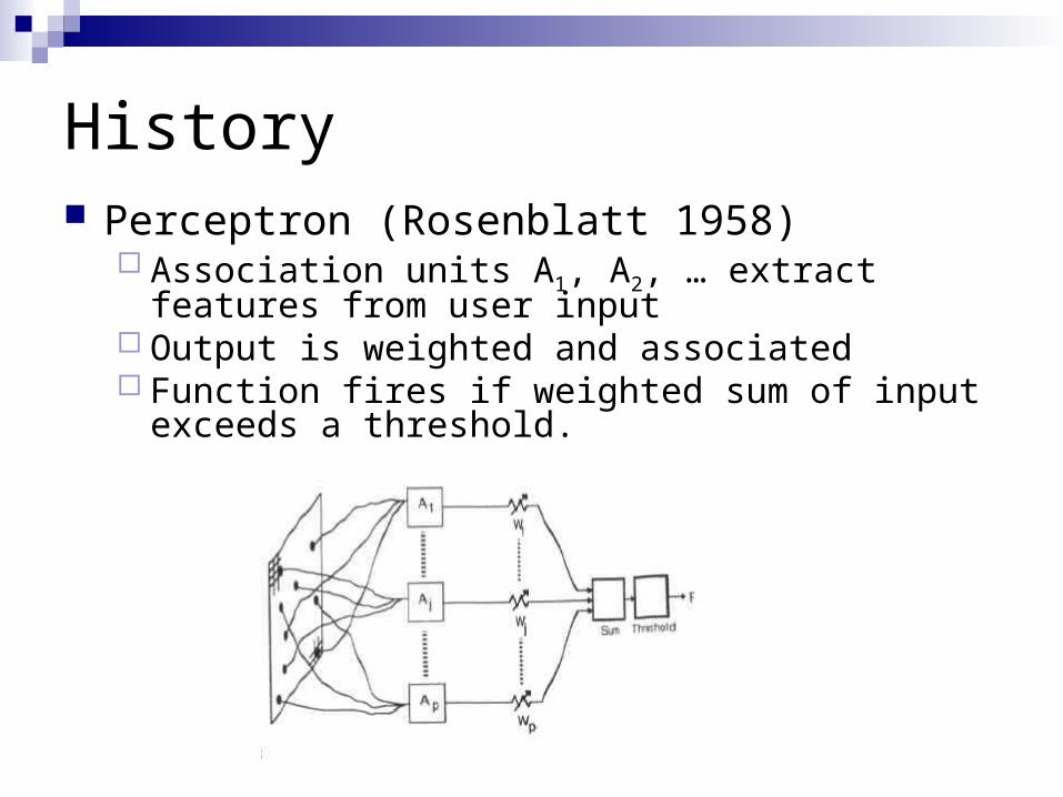
History Perceptron (Rosenblatt 1958)
Association units A1, A2, … extract features from user input
Output is weighted and associated Function fires if weighted sum of input exceeds a
threshold.
History
Back-propagation learning method (Werbos 1974) Three layers of neurons
Input, Output, Hidden Better learning rule for generic three layer networks Regenerates interest in the 1980s
Successful applications in medicine, marketing, risk management, … (1990)
In need for another breakthrough.

ANN
PromisesCombine speed of silicon with proven success
of carbon artificial brains
Neuron Model
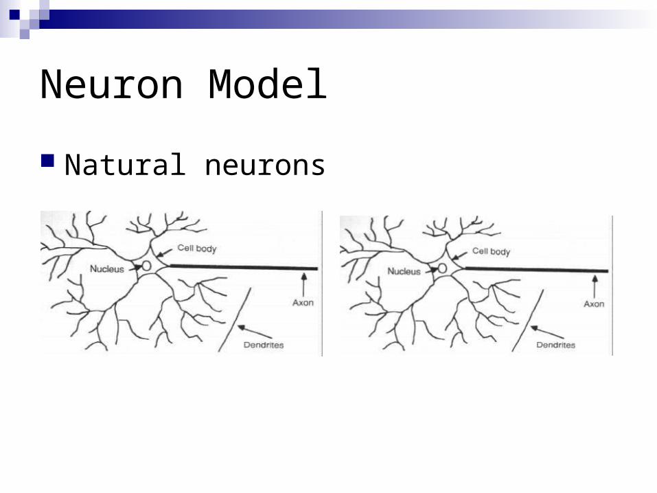
Natural neurons
Neuron Model
Neuron collects signals from dendrites Sends out spikes of electrical activity through an
axon, which splits into thousands of branches. At end of each brand, a synapses converts
activity into either exciting or inhibiting activity of a dendrite at another neuron.
Neuron fires when exciting activity surpasses inhibitory activity
Learning changes the effectiveness of the synapses

Neuron Model
Natural neurons

Neuron Model
Abstract neuron model:

ANN Forward Propagation
ANN Forward Propagation
Bias NodesAdd one node to each layer that has constant
output Forward propagation
Calculate from input layer to output layerFor each neuron:
Calculate weighted average of input Calculate activation function
Neuron Model
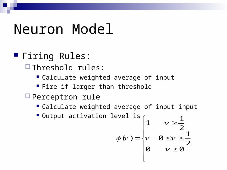
Firing Rules: Threshold rules:
Calculate weighted average of input Fire if larger than threshold
Perceptron rule Calculate weighted average of input input Output activation level is
002
10
2
11
)(

Neuron Model
Firing Rules: Sigmoid functions:Hyperbolic tangent function
Logistic activation function
)exp(1
)exp(1)2/tanh(
exp1
1

ANN Forward Propagation
ANN Forward Propagation
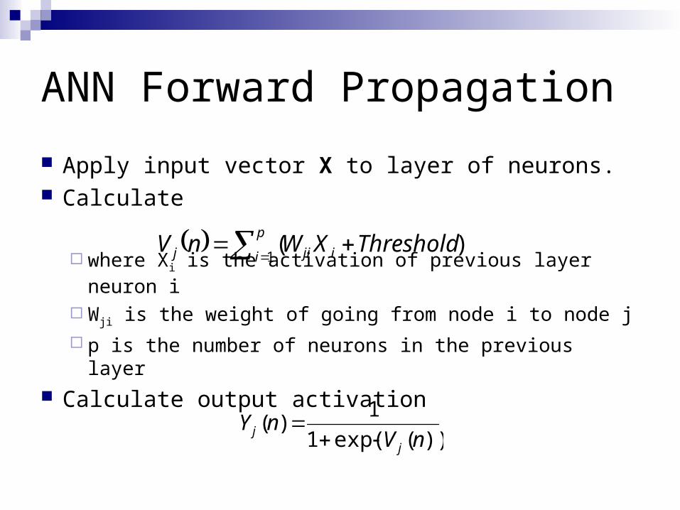
Apply input vector X to layer of neurons. Calculate
where Xi is the activation of previous layer neuron i
Wji is the weight of going from node i to node j
p is the number of neurons in the previous layer
Calculate output activation
)(1
ThresholdXWnV i
p
i jij
))(exp(1
1)(
nVnY
jj
ANN Forward Propagation
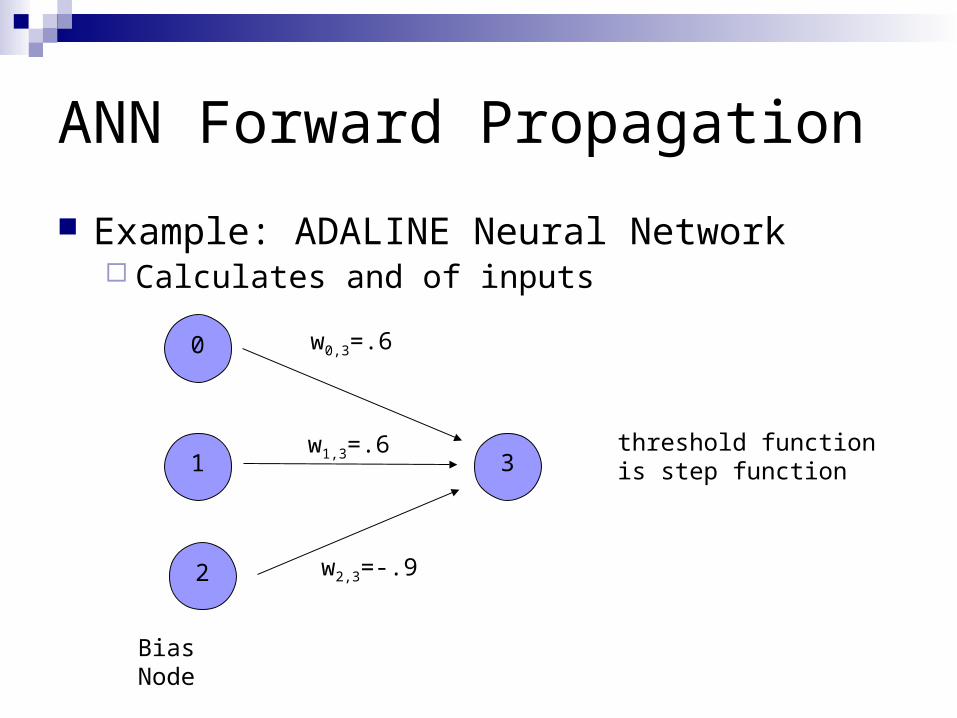
Example: ADALINE Neural Network Calculates and of inputs
0
1
2
Bias Node
3
w0,3=.6
w1,3=.6
w2,3=-.9
threshold function is step function
ANN Forward Propagation
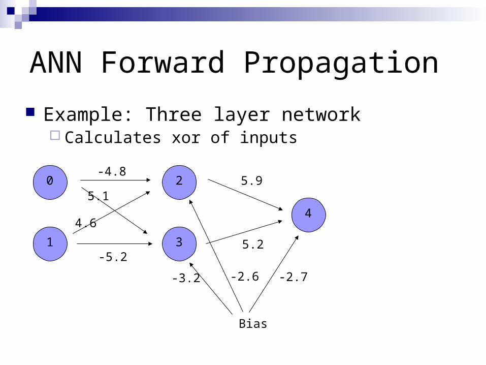
Example: Three layer network Calculates xor of inputs
0
1
2
3
4
-4.8
-5.2
4.6
5.15.9
5.2
-2.7-2.6-3.2
Bias
ANN Forward Propagation
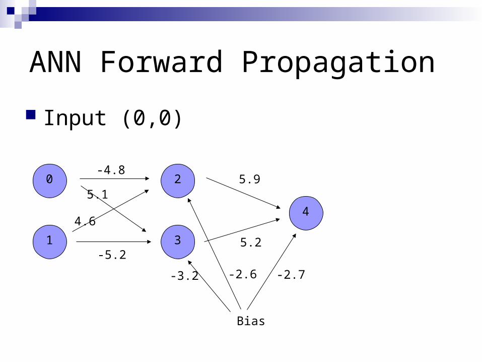
Input (0,0)
0
1
2
3
4
-4.8
-5.2
4.6
5.15.9
5.2
-2.7-2.6-3.2
Bias
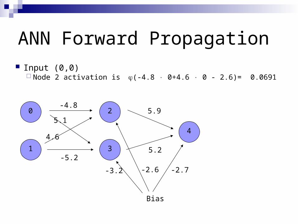
ANN Forward Propagation
Input (0,0) Node 2 activation is (-4.8 0+4.6 0 - 2.6)= 0.0691
0
1
2
3
4
-4.8
-5.2
4.6
5.15.9
5.2
-2.7-2.6-3.2
Bias
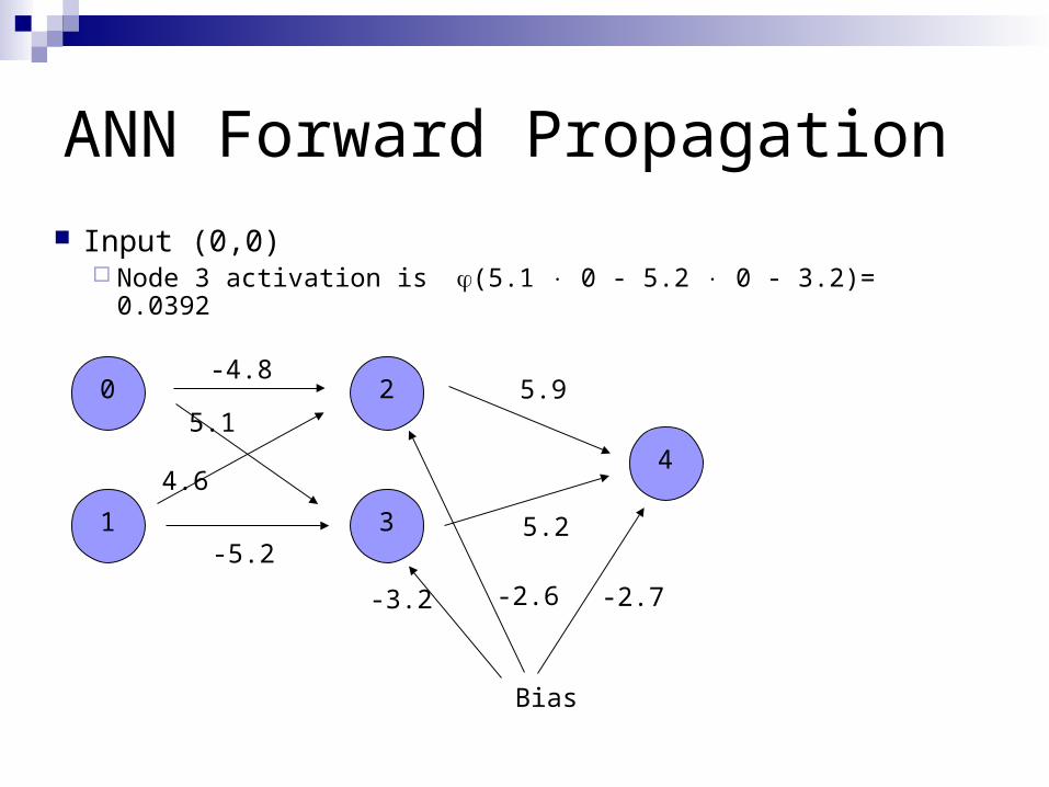
ANN Forward Propagation
Input (0,0) Node 3 activation is (5.1 0 - 5.2 0 - 3.2)= 0.0392
0
1
2
3
4
-4.8
-5.2
4.6
5.15.9
5.2
-2.7-2.6-3.2
Bias
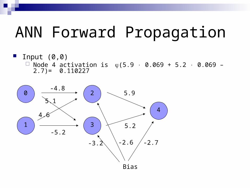
ANN Forward Propagation Input (0,0)
Node 4 activation is (5.9 0.069 + 5.2 0.069 – 2.7)= 0.110227
0
1
2
3
4
-4.8
-5.2
4.6
5.15.9
5.2
-2.7-2.6-3.2
Bias
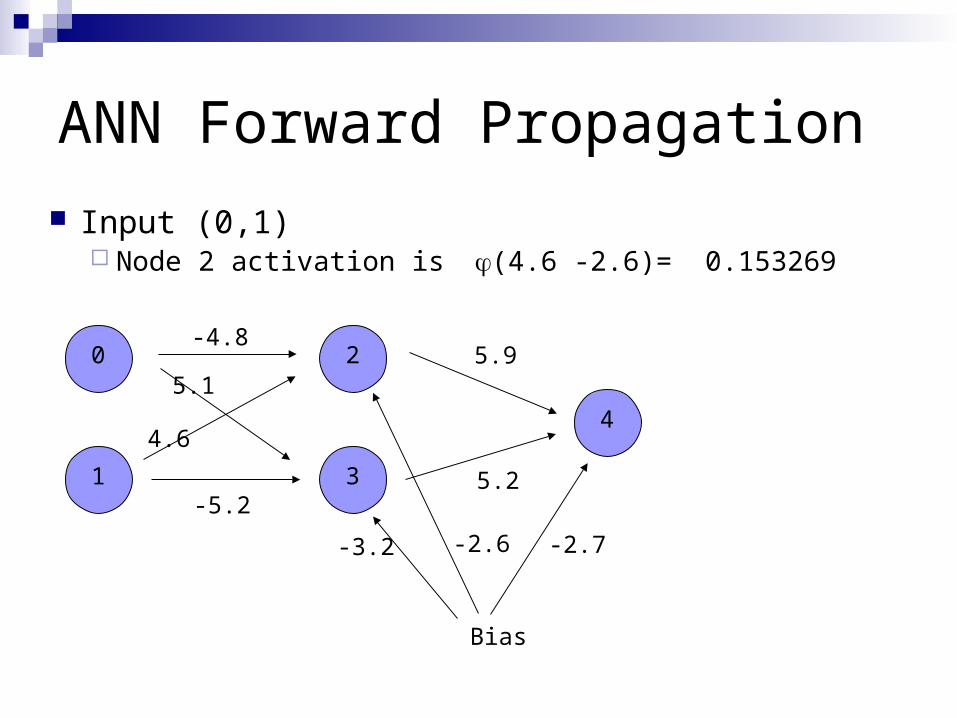
ANN Forward Propagation
Input (0,1) Node 2 activation is (4.6 -2.6)= 0.153269
0
1
2
3
4
-4.8
-5.2
4.6
5.15.9
5.2
-2.7-2.6-3.2
Bias

ANN Forward Propagation
Input (0,1) Node 3 activation is (-5.2 -3.2)= 0.000224817
0
1
2
3
4
-4.8
-5.2
4.6
5.15.9
5.2
-2.7-2.6-3.2
Bias
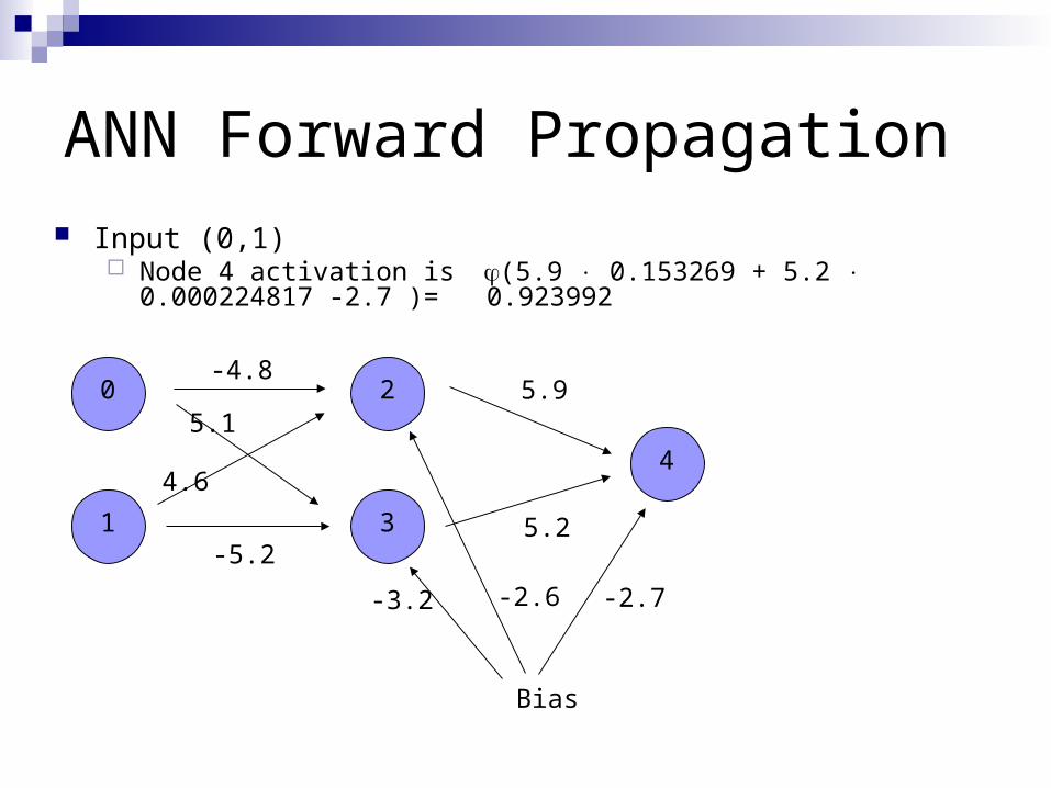
ANN Forward Propagation Input (0,1)
Node 4 activation is (5.9 0.153269 + 5.2 0.000224817 -2.7 )= 0.923992
0
1
2
3
4
-4.8
-5.2
4.6
5.15.9
5.2
-2.7-2.6-3.2
Bias
ANN Forward Propagation
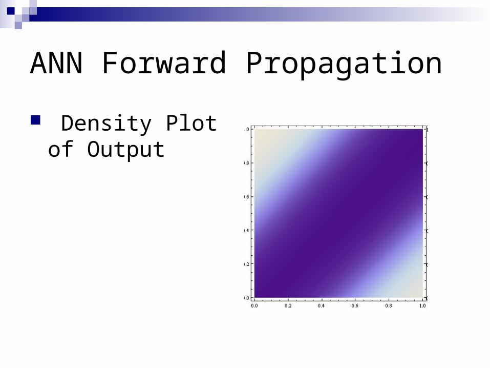
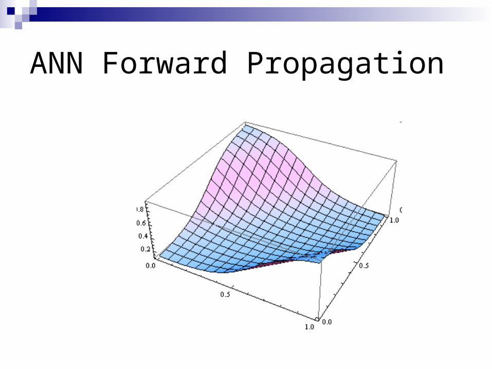
Density Plot of Output
ANN Forward Propagation
ANN Forward Propagation
Network can learn a non-linearly separated set of outputs.
Need to map output (real value) into binary values.
ANN Training
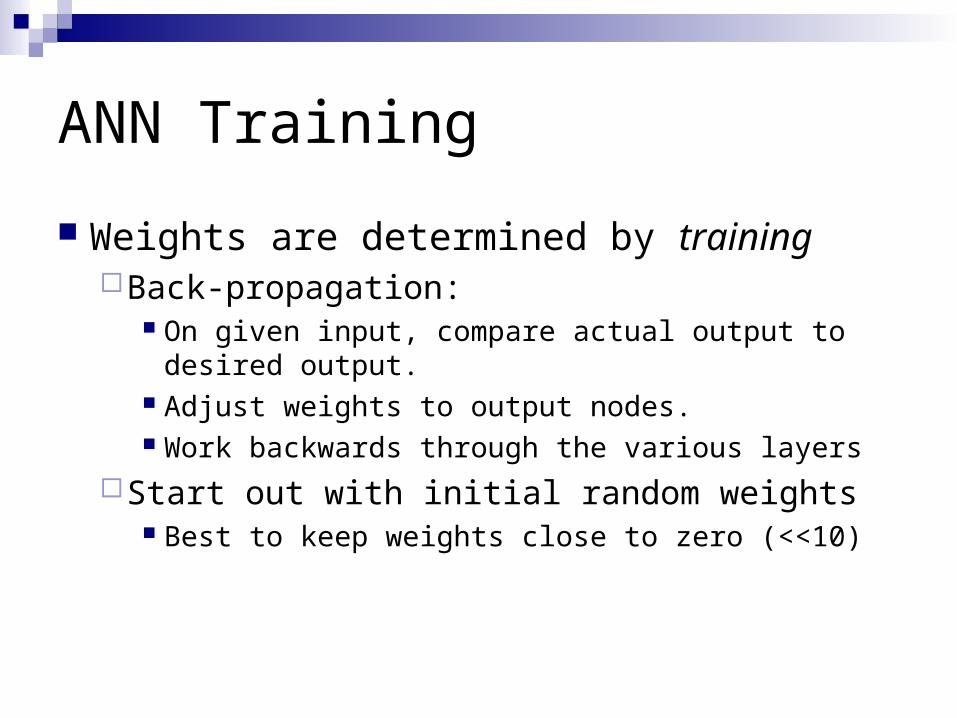
Weights are determined by trainingBack-propagation:
On given input, compare actual output to desired output.
Adjust weights to output nodes. Work backwards through the various layers
Start out with initial random weights Best to keep weights close to zero (<<10)

ANN Training
Weights are determined by trainingNeed a training set
Should be representative of the problem
During each training epoch: Submit training set element as input Calculate the error for the output neurons Calculate average error during epoch Adjust weights
ANN Training
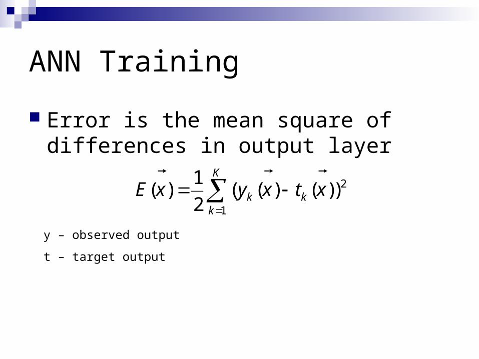
Error is the mean square of differences in output layer
2
1
))()((2
1)(
K
kkk xtxyxE
y – observed output
t – target output
ANN Training
Error of training epoch is the average of all errors.
ANN Training
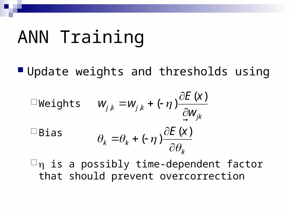
Update weights and thresholds using
Weights
Bias
is a possibly time-dependent factor that should prevent overcorrection
kkk
jkkjkj
xE
w
xEww
)()(
)()(,,
ANN Training
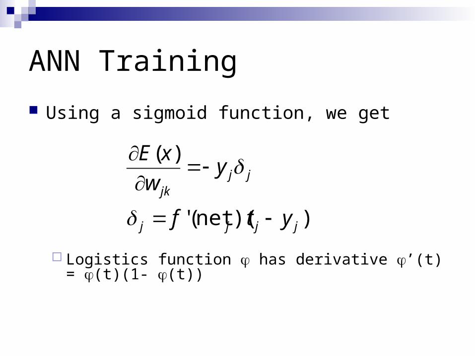
Using a sigmoid function, we get
Logistics function has derivative ’(t) = (t)(1- (t))
))(net('
)(
jjjj
jjjk
ytf
yw
xE
ANN Training Example
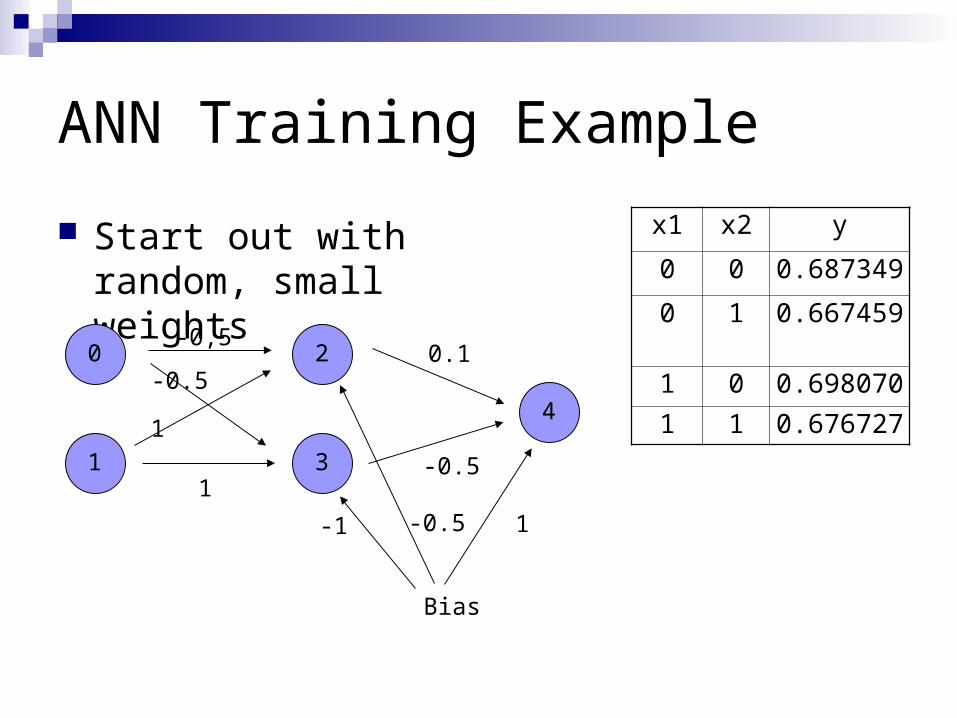
Start out with random, small weights
0
1
2
3
4
-0,5
1
1
-0.50.1
-0.5
1-0.5-1
Bias
x1 x2 y
0 0 0.687349
0 1 0.667459
1 0 0.698070
1 1 0.676727

ANN Training Example
0
1
2
3
4
-0,5
1
1
-0.50.1
-0.5
1-0.5-1
Bias
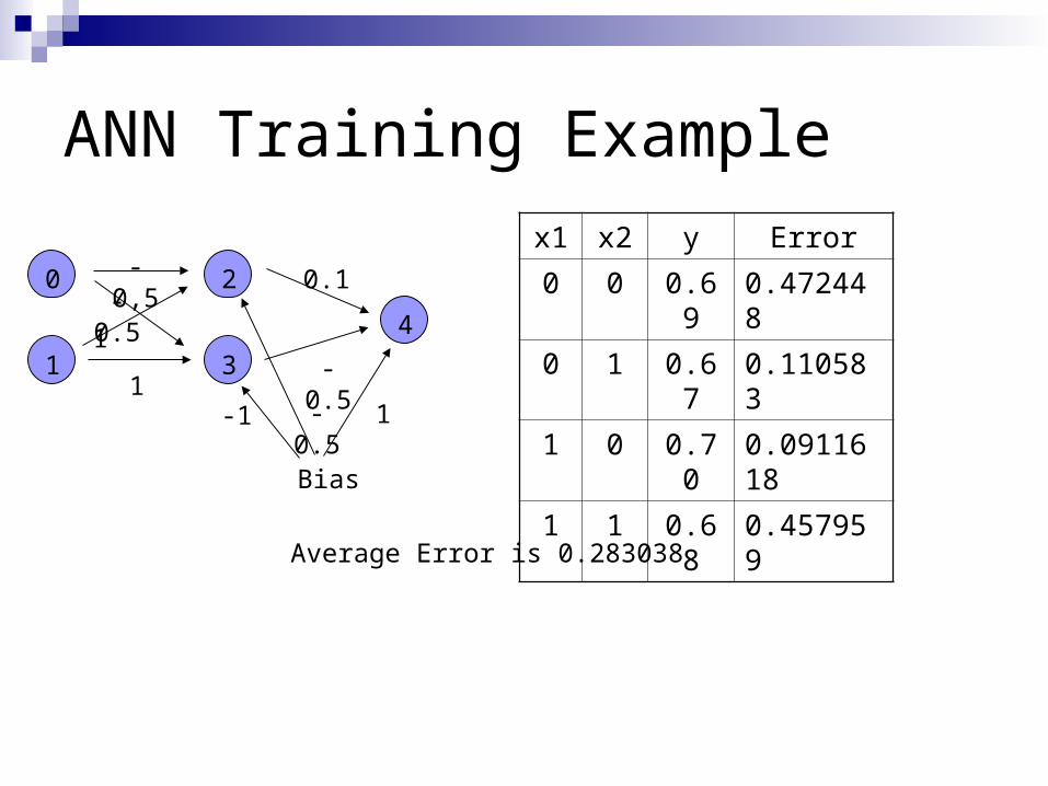
x1 x2 y Error
0 0 0.69 0.472448
0 1 0.67 0.110583
1 0 0.70 0.0911618
1 1 0.68 0.457959
Average Error is 0.283038
ANN Training Example
0
1
2
3
4
-0,5
1
1
-0.50.1
-0.5
1-0.5-1
Bias
x1 x2 y Error
0 0 0.69 0.472448
0 1 0.67 0.110583
1 0 0.70 0.0911618
1 1 0.68 0.457959
Average Error is 0.283038
ANN Training Example
Calculate the derivative of the error with respect to the weights and bias into the output layer neurons
ANN Training Example
0
1
2
3
4
-0,5
1
1
-0.50.1
-0.5
1-0.5-1
Bias
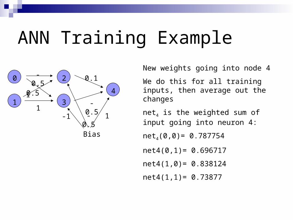
New weights going into node 4
We do this for all training inputs, then average out the changes
net4 is the weighted sum of input going into neuron 4:
net4(0,0)= 0.787754
net4(0,1)= 0.696717
net4(1,0)= 0.838124
net4(1,1)= 0.73877
ANN Training Example
0
1
2
3
4
-0,5
1
1
-0.50.1
-0.5
1-0.5-1
Bias
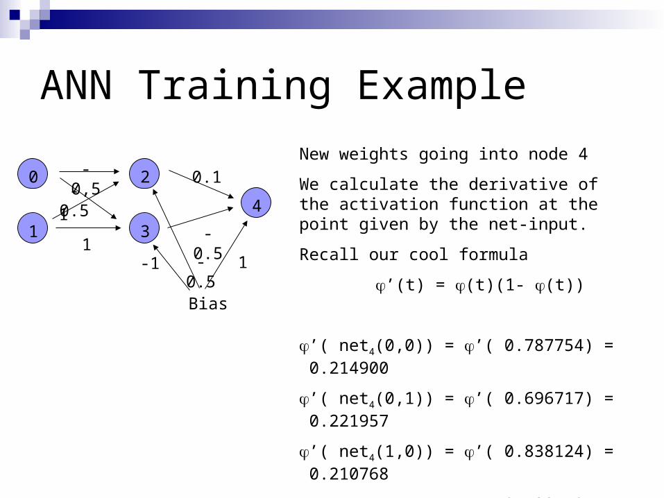
New weights going into node 4
We calculate the derivative of the activation function at the point given by the net-input.
Recall our cool formula
’(t) = (t)(1- (t))
’( net4(0,0)) = ’( 0.787754) = 0.214900
’( net4(0,1)) = ’( 0.696717) = 0.221957
’( net4(1,0)) = ’( 0.838124) = 0.210768
’( net4(1,1)) = ’( 0.738770) = 0.218768
ANN Training Example
0
1
2
3
4
-0,5
1
1
-0.50.1
-0.5
1-0.5-1
Bias
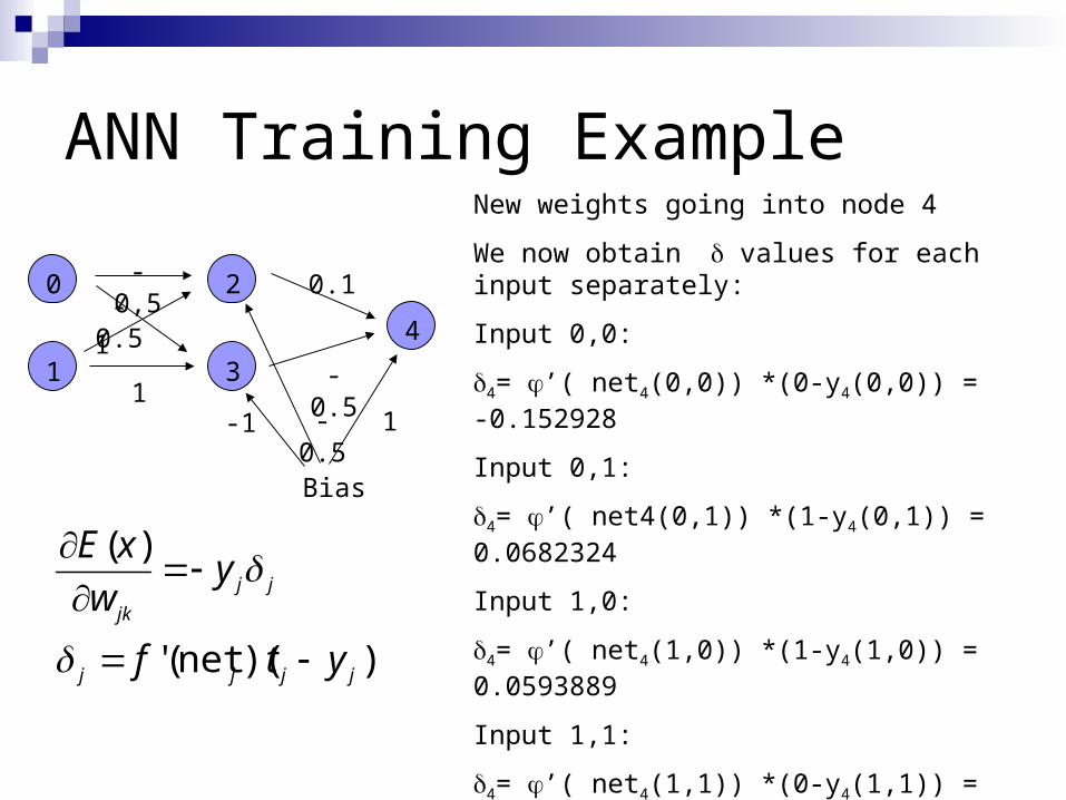
New weights going into node 4
We now obtain values for each input separately:
Input 0,0:
4= ’( net4(0,0)) *(0-y4(0,0)) = -0.152928
Input 0,1:
4= ’( net4(0,1)) *(1-y4(0,1)) = 0.0682324
Input 1,0:
4= ’( net4(1,0)) *(1-y4(1,0)) = 0.0593889
Input 1,1:
4= ’( net4(1,1)) *(0-y4(1,1)) = -0.153776
Average: 4 = -0.0447706
))(net('
)(
jjjj
jj
jk
ytf
yw
xE
ANN Training Example
0
1
2
3
4
-0,5
1
1
-0.50.1
-0.5
1-0.5-1
Bias
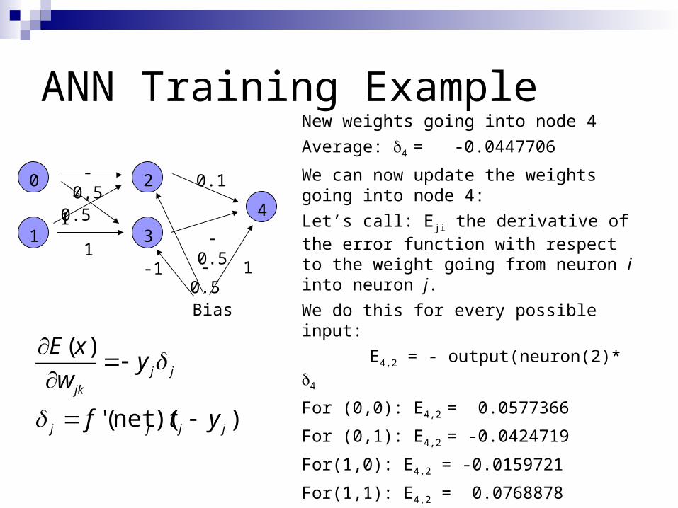
New weights going into node 4
Average: 4 = -0.0447706
We can now update the weights going into node 4:
Let’s call: Eji the derivative of the error function with respect to the weight going from neuron i into neuron j.
We do this for every possible input:
E4,2 = - output(neuron(2)* 4
For (0,0): E4,2 = 0.0577366
For (0,1): E4,2 = -0.0424719
For(1,0): E4,2 = -0.0159721
For(1,1): E4,2 = 0.0768878
Average is 0.0190451
))(net('
)(
jjjj
jj
jk
ytf
yw
xE
ANN Training Example
0
1
2
3
4
-0,5
1
1
-0.50.1
-0.5
1-0.5-1
Bias
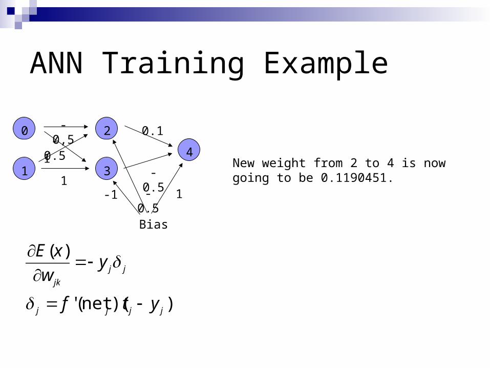
New weight from 2 to 4 is now going to be 0.1190451.
))(net('
)(
jjjj
jj
jk
ytf
yw
xE
ANN Training Example
0
1
2
3
4
-0,5
1
1
-0.50.1
-0.5
1-0.5-1
Bias
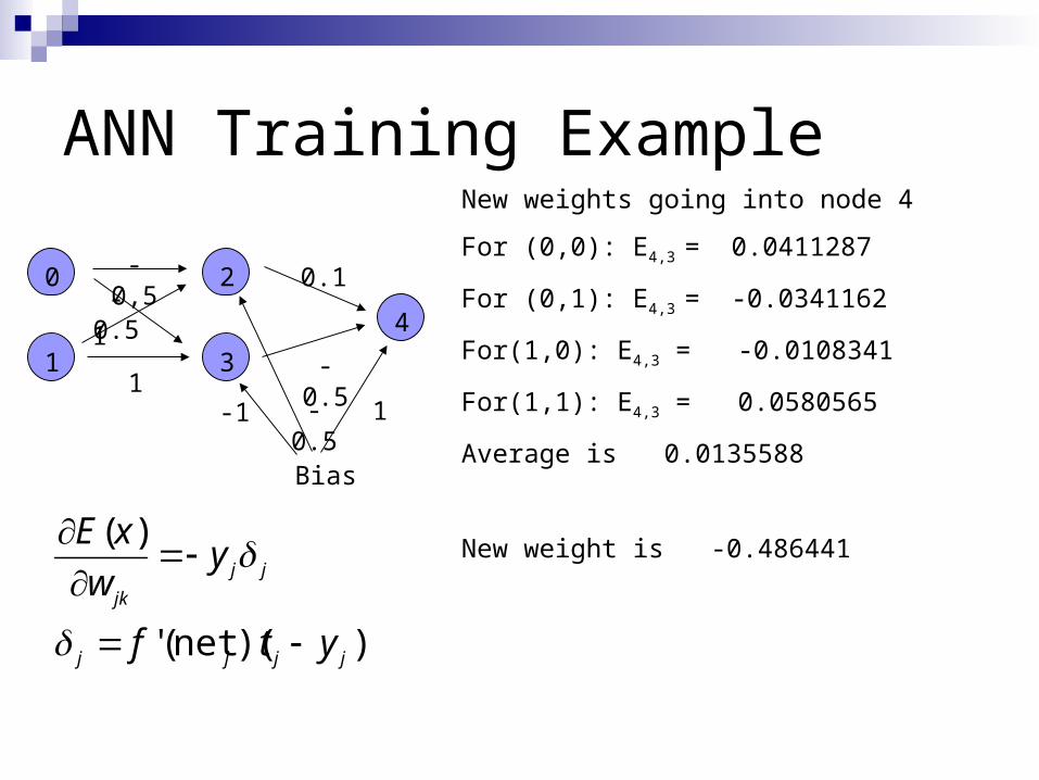
New weights going into node 4
For (0,0): E4,3 = 0.0411287
For (0,1): E4,3 = -0.0341162
For(1,0): E4,3 = -0.0108341
For(1,1): E4,3 = 0.0580565
Average is 0.0135588
New weight is -0.486441
))(net('
)(
jjjj
jj
jk
ytf
yw
xE

ANN Training Example
0
1
2
3
4
-0,5
1
1
-0.50.1
-0.5
1-0.5-1
Bias
New weights going into node 4:
We also need to change the bias node
For (0,0): E4,B = 0.0411287
For (0,1): E4,B = -0.0341162
For(1,0): E4,B = -0.0108341
For(1,1): E4,B = 0.0580565
Average is 0.0447706
New weight is 1.0447706
))(net('
)(
jjjj
jj
jk
ytf
yw
xE
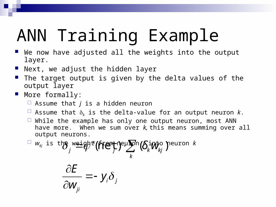
ANN Training Example We now have adjusted all the weights into the output layer. Next, we adjust the hidden layer The target output is given by the delta values of the output layer More formally:
Assume that j is a hidden neuron Assume that k is the delta-value for an output neuron k. While the example has only one output neuron, most ANN have more.
When we sum over k, this means summing over all output neurons. wkj is the weight from neuron j into neuron k
ji
ji
kkjkjj
yw
E
wδ
)()net('
ANN Training Example
0
1
2
3
4
-0,5
1
1
-0.50.1
-0.5
1-0.5-1
Bias
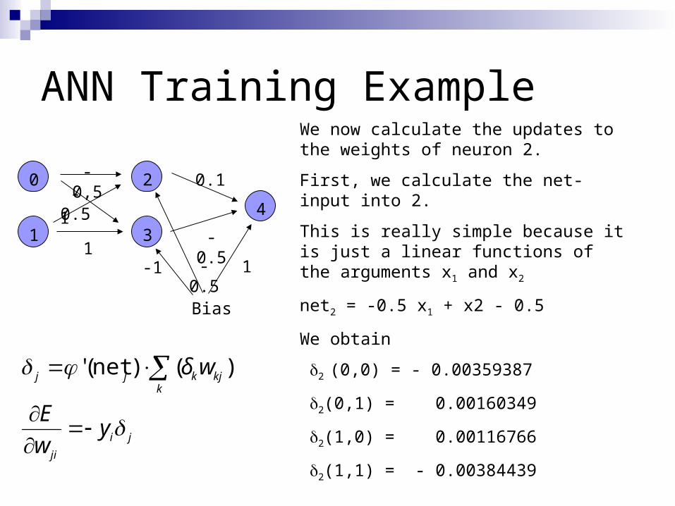
We now calculate the updates to the weights of neuron 2.
First, we calculate the net-input into 2.
This is really simple because it is just a linear functions of the arguments x1 and x2
net2 = -0.5 x1 + x2 - 0.5
We obtain
2 (0,0) = - 0.00359387
2(0,1) = 0.00160349
2(1,0) = 0.00116766
2(1,1) = - 0.00384439ji
ji
kkjkjj
yw
E
wδ
)()net('
ANN Training Example
0
1
2
3
4
-0,5
1
1
-0.50.1
-0.5
1-0.5-1
Bias
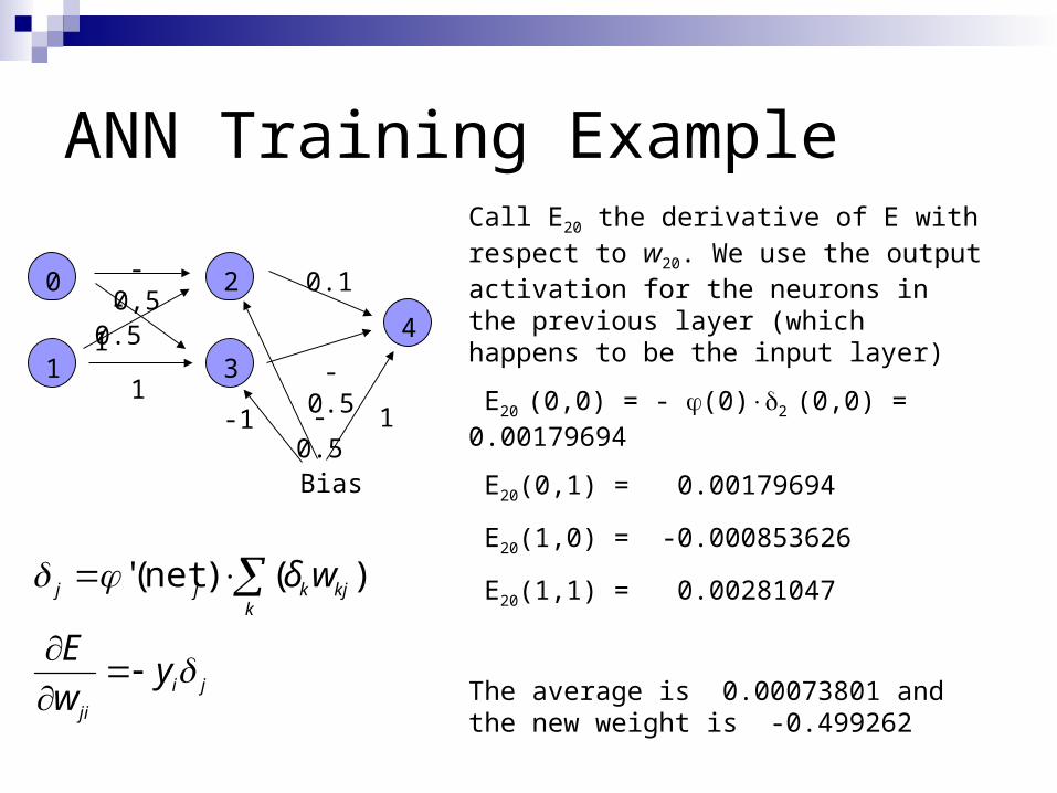
Call E20 the derivative of E with respect to w20. We use the output activation for the neurons in the previous layer (which happens to be the input layer)
E20 (0,0) = - (0)2 (0,0) = 0.00179694
E20(0,1) = 0.00179694
E20(1,0) = -0.000853626
E20(1,1) = 0.00281047
The average is 0.00073801 and the new weight is -0.499262
ji
ji
kkjkjj
yw
E
wδ
)()net('
ANN Training Example
0
1
2
3
4
-0,5
1
1
-0.50.1
-0.5
1-0.5-1
Bias
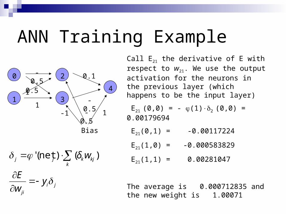
Call E21 the derivative of E with respect to w21. We use the output activation for the neurons in the previous layer (which happens to be the input layer)
E21 (0,0) = - (1)2 (0,0) = 0.00179694
E21(0,1) = -0.00117224
E21(1,0) = -0.000583829
E21(1,1) = 0.00281047
The average is 0.000712835 and the new weight is 1.00071
ji
ji
kkjkjj
yw
E
wδ
)()net('
ANN Training Example
0
1
2
3
4
-0,5
1
1
-0.50.1
-0.5
1-0.5-1
Bias
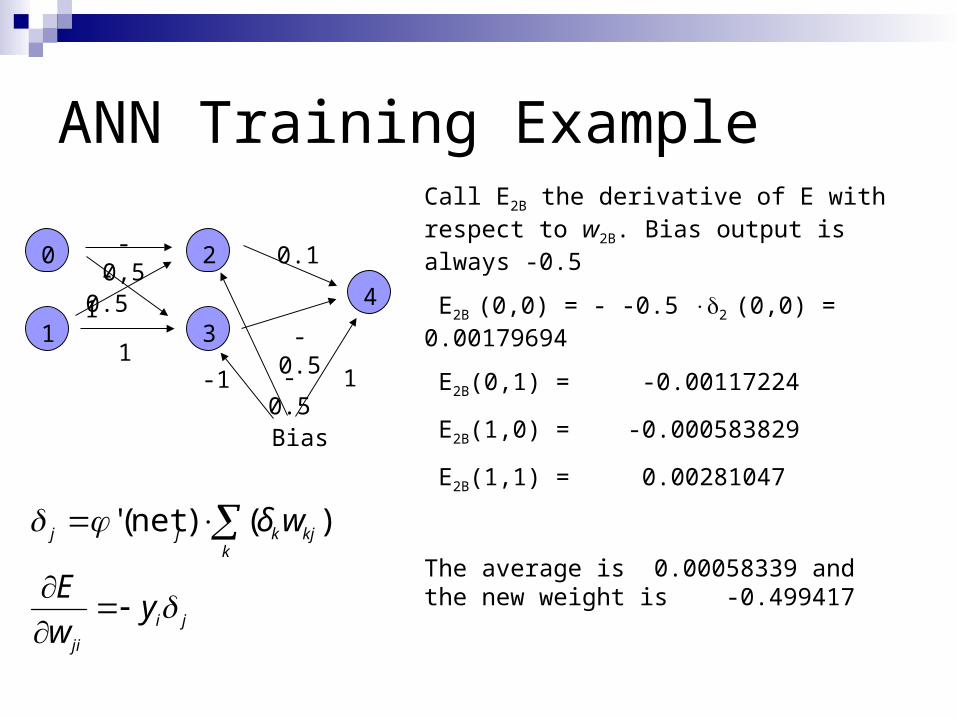
Call E2B the derivative of E with respect to w2B. Bias output is always -0.5
E2B (0,0) = - -0.5 2 (0,0) = 0.00179694
E2B(0,1) = -0.00117224
E2B(1,0) = -0.000583829
E2B(1,1) = 0.00281047
The average is 0.00058339 and the new weight is -0.499417
ji
ji
kkjkjj
yw
E
wδ
)()net('
ANN Training Example
0
1
2
3
4
-0,5
1
1
-0.50.1
-0.5
1-0.5-1
Bias
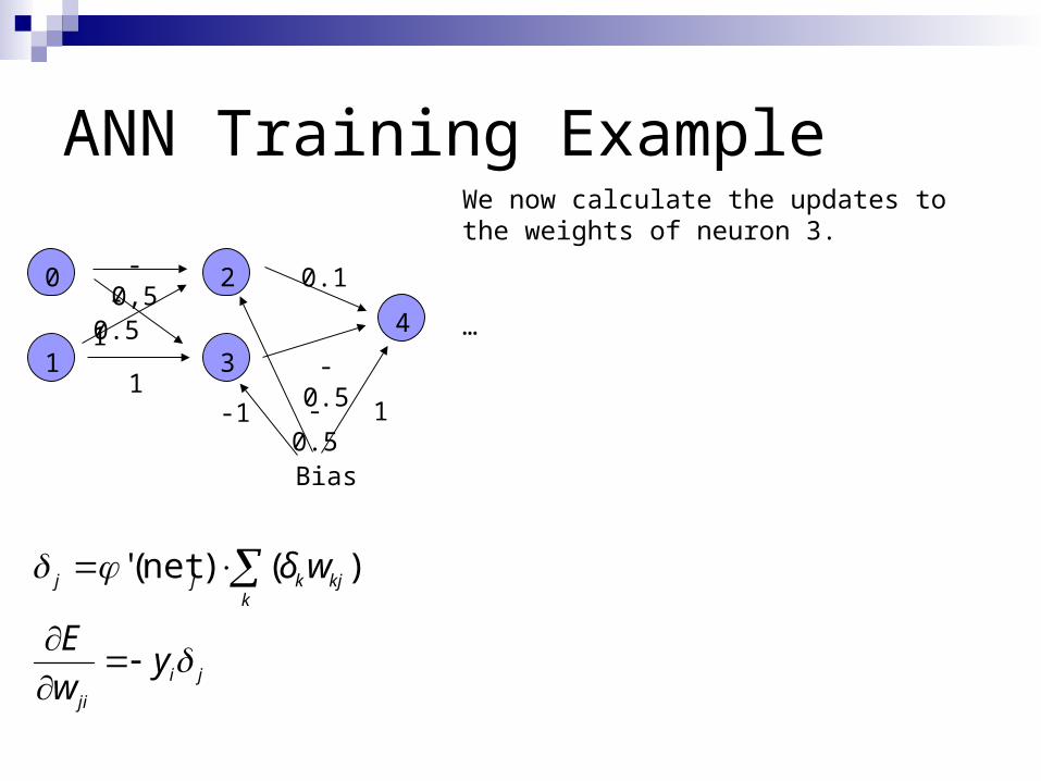
We now calculate the updates to the weights of neuron 3.
…
ji
ji
kkjkjj
yw
E
wδ
)()net('
ANN Training
ANN Back-propagation is an empirical algorithm
ANN Training
XOR is too simple an example, since quality of ANN is measured on a finite sets of inputs.
More relevant are ANN that are trained on a training set and unleashed on real data
ANN Training
Need to measure effectiveness of training Need training sets Need test sets.
There can be no interaction between test sets and training sets. Example of a Mistake:
Train ANN on training set. Test ANN on test set. Results are poor. Go back to training ANN.
After this, there is no assurance that ANN will work well in practice.
In a subtle way, the test set has become part of the training set.
ANN Training
Convergence ANN back propagation uses gradient decent. Naïve implementations can
overcorrect weights undercorrect weights
In either case, convergence can be poor Stuck in the wrong place
ANN starts with random weights and improves them If improvement stops, we stop algorithm No guarantee that we found the best set of weights Could be stuck in a local minimum
ANN Training
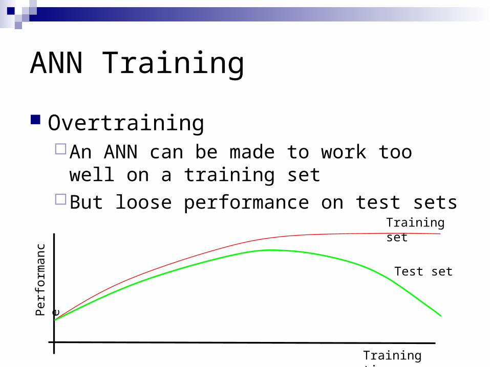
OvertrainingAn ANN can be made to work too well on a
training setBut loose performance on test sets
Training set
Test set
Per
form
ance
Training time
ANN Training
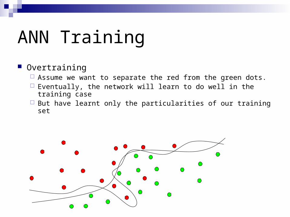
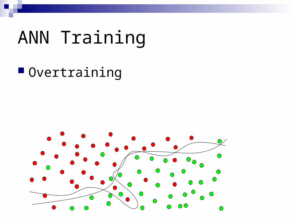
Overtraining Assume we want to separate the red from the green dots. Eventually, the network will learn to do well in the training case But have learnt only the particularities of our training set
ANN Training
Overtraining

ANN Training
Improving ConvergenceMany Operations Research Tools apply
Simulated annealing Sophisticated gradient descent
ANN Design
ANN is a largely empirical study“Seems to work in almost all cases that we
know about” Known to be statistical pattern analysis
ANN Design
Number of layers Apparently, three layers is almost always good
enough and better than four layers. Also: fewer layers are faster in execution and training
How many hidden nodes? Many hidden nodes allow to learn more complicated
patterns Because of overtraining, almost always best to set the
number of hidden nodes too low and then increase their numbers.

ANN Design
Interpreting OutputANN’s output neurons do not give binary
values. Good or bad Need to define what is an accept.
Can indicate n degrees of certainty with n-1 output neurons.
Number of firing output neurons is degree of certainty
ANN Applications
Pattern recognition Network attacks Breast cancer … handwriting recognition
Pattern completion Auto-association
ANN trained to reproduce input as output Noise reduction Compression Finding anomalies
Time Series Completion
ANN Future
ANNs can do some things really well They lack in structure found in most
natural neural networks
Pseudo-Code
phi – activation function phid – derivative of activation function

Pseudo-Code
Forward Propagation: Input nodes i, given input xi:
foreach inputnode i
outputi = xi
Hidden layer nodes jforeach hiddenneuron j
outputj = i phi(wjioutputi) Output layer neurons k
foreach outputneuron k
outputk = k phi(wkjoutputj)
Pseudo-Code
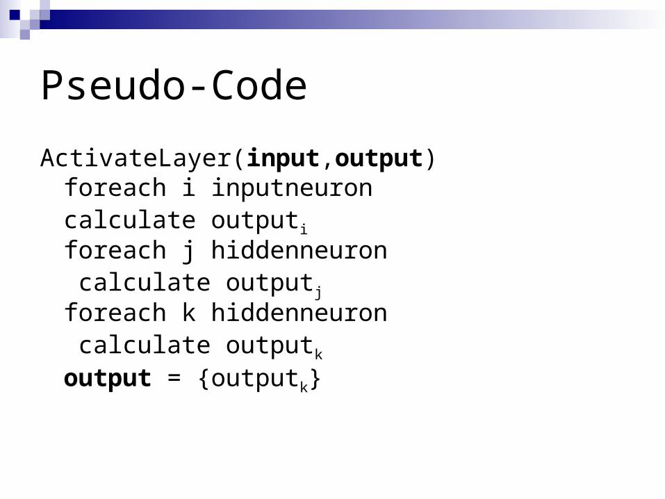
ActivateLayer(input,output)foreach i inputneuron
calculate outputi
foreach j hiddenneuron calculate outputj
foreach k hiddenneuron calculate outputk
output = {outputk}
Pseudo-Code
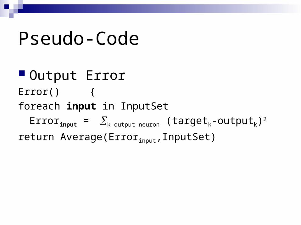
Output ErrorError() {
foreach input in InputSet
Errorinput = k output neuron (targetk-outputk)2
return Average(Errorinput,InputSet)
Pseudo-Code
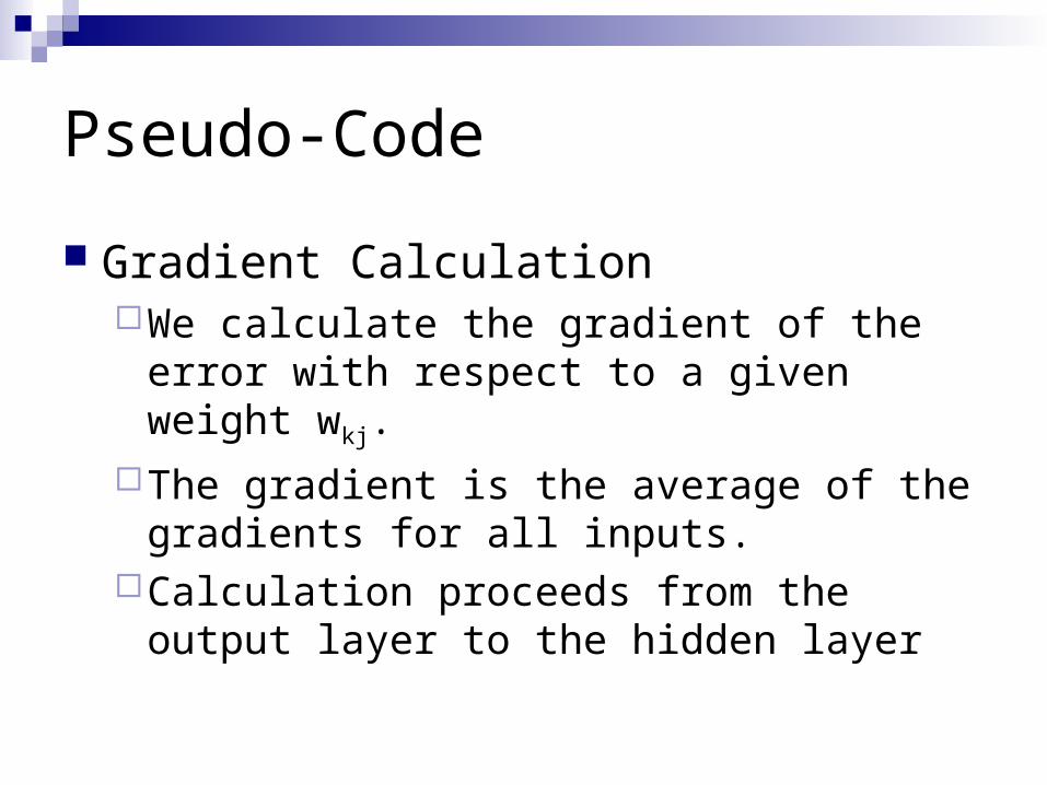
Gradient CalculationWe calculate the gradient of the error with
respect to a given weight wkj.
The gradient is the average of the gradients for all inputs.
Calculation proceeds from the output layer to the hidden layer
Pseudo-Code
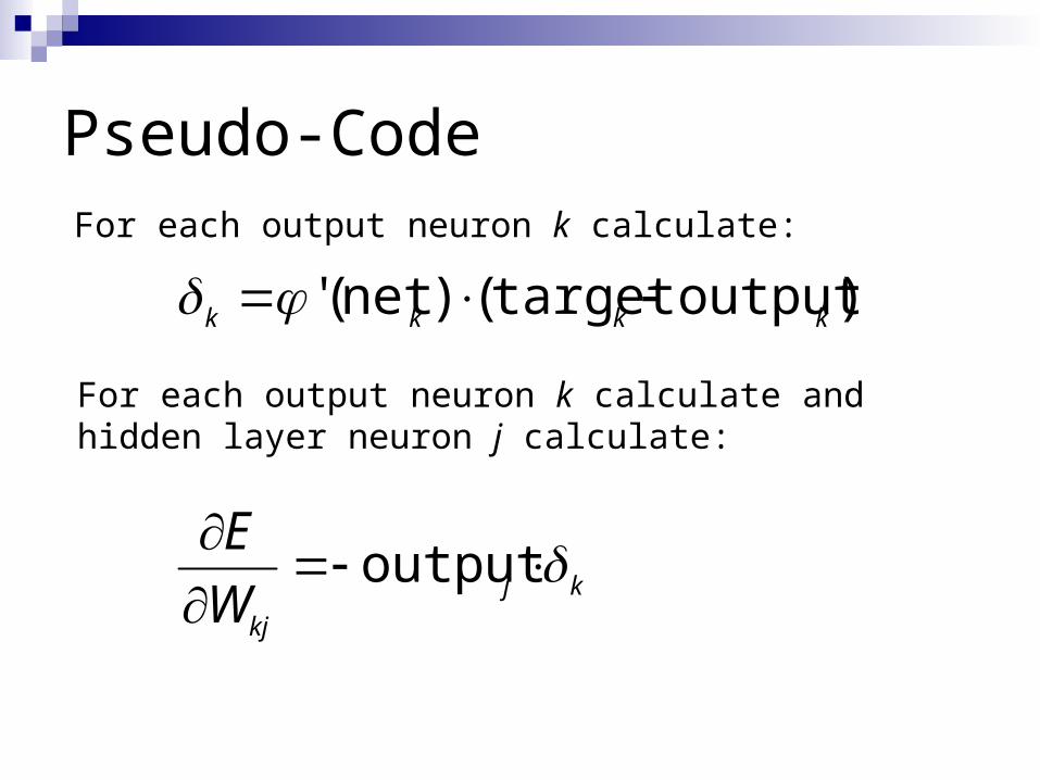
kj
kj
kkkk
W
E
output
)outputtarget()net('
For each output neuron k calculate:
For each output neuron k calculate and hidden layer neuron j calculate:
Pseudo-Code
k kjkjj W )net('
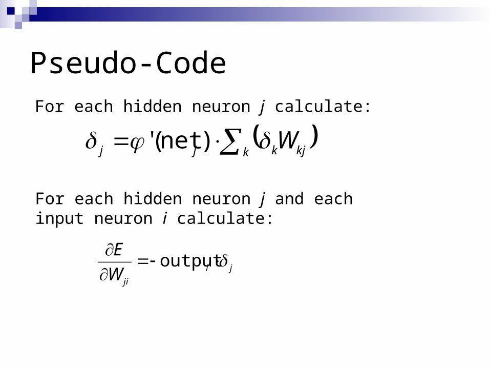
For each hidden neuron j calculate:
For each hidden neuron j and each input neuron i calculate:
ji
jiW
E
output

Pseudo-Code
These calculations were done for a single input.
Now calculate the average gradient over all inputs (and for all weights).
You also need to calculate the gradients for the bias weights and average them.
Pseudo-Code
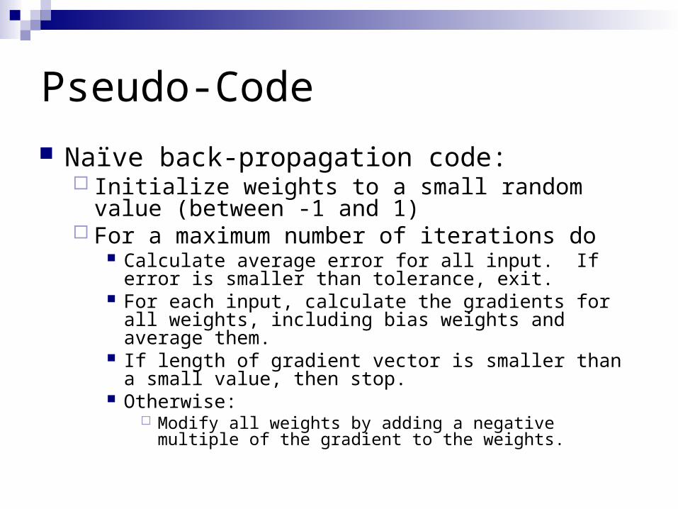
Naïve back-propagation code: Initialize weights to a small random value (between -1
and 1) For a maximum number of iterations do
Calculate average error for all input. If error is smaller than tolerance, exit.
For each input, calculate the gradients for all weights, including bias weights and average them.
If length of gradient vector is smaller than a small value, then stop.
Otherwise: Modify all weights by adding a negative multiple of the gradient
to the weights.
Pseudo-Code
This naïve algorithm has problems with convergence and should only be used for toy problems.