ArCo: An Artificial Counterfactual Approach for High ... · ArCo: An Artificial Counterfactual...
92
ArCo: An Artificial Counterfactual Approach for High-Dimensional Data Carlos V. de Carvalho BCB and PUC-Rio Marcelo C. Medeiros PUC-Rio Ricardo Masini São Paulo School of Economics BIG DATA, MACHINE LEARNING AND THE MACROECONOMY Norges Bank, Oslo, 2-3 October 2017
-
Upload
duongthuan -
Category
Documents
-
view
222 -
download
1
Transcript of ArCo: An Artificial Counterfactual Approach for High ... · ArCo: An Artificial Counterfactual...

ArCo: An Artificial Counterfactual Approach forHigh-Dimensional Data
Carlos V. de CarvalhoBCB and PUC-Rio
Marcelo C. MedeirosPUC-Rio
Ricardo MasiniSão Paulo School of Economics
BIG DATA, MACHINE LEARNING AND THEMACROECONOMY
Norges Bank, Oslo, 2-3 October 2017
Overview of the Method
Observe aggregated time series data from t = 1 to T .
0 10 20 30 40 50 60 70 80
time-0.6
-0.4
-0.2
0
0.2
0.4
0.6
0.8
1
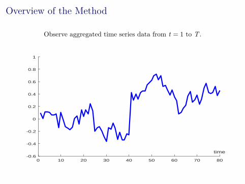
Overview of the Method
Intervention occurs at t = T0.
0 10 20 30 40 50 60 70 80
time-0.6
-0.4
-0.2
0
0.2
0.4
0.6
0.8
1
T0
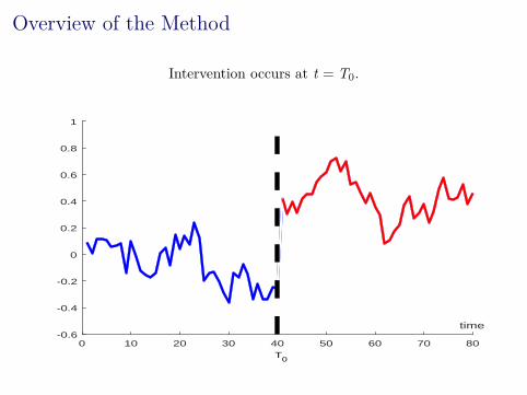
Overview of the Method
No clear controls. Observed variables from untreated “peers”.
0 10 20 30 40 50 60 70 80
time-0.6
-0.4
-0.2
0
0.2
0.4
0.6
0.8
1
T0
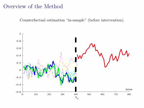
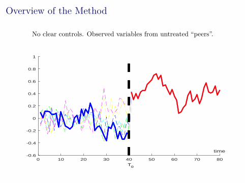
Overview of the Method
Counterfactual estimation “in-sample” (before intervention).
0 10 20 30 40 50 60 70 80
time-0.6
-0.4
-0.2
0
0.2
0.4
0.6
0.8
1
T0
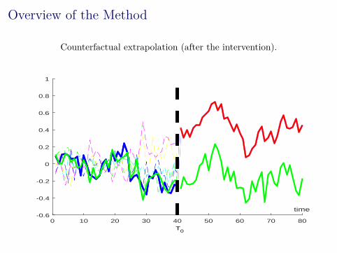
Overview of the Method
Counterfactual extrapolation (after the intervention).
0 10 20 30 40 50 60 70 80
time-0.6
-0.4
-0.2
0
0.2
0.4
0.6
0.8
1
T0

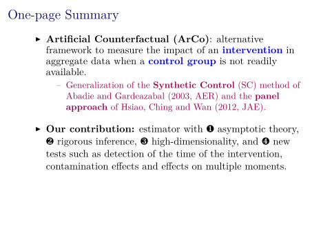
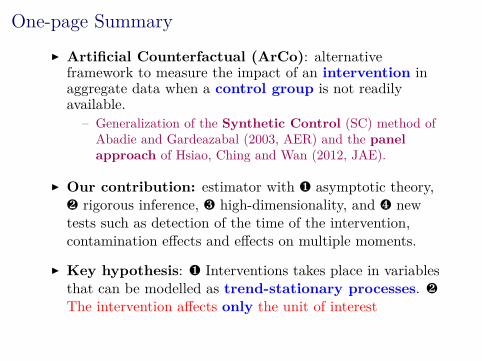
One-page Summary Artificial Counterfactual (ArCo): alternative
framework to measure the impact of an intervention inaggregate data when a control group is not readilyavailable.
– Generalization of the Synthetic Control (SC) method ofAbadie and Gardeazabal (2003, AER) and the panelapproach of Hsiao, Ching and Wan (2012, JAE).
Our contribution: estimator with ¶ asymptotic theory,· rigorous inference, ¸ high-dimensionality, and ¹ newtests such as detection of the time of the intervention,contamination effects and effects on multiple moments.
Key hypothesis: ¶ Interventions takes place in variablesthat can be modelled as trend-stationary processes. ·
The intervention affects only the unit of interest
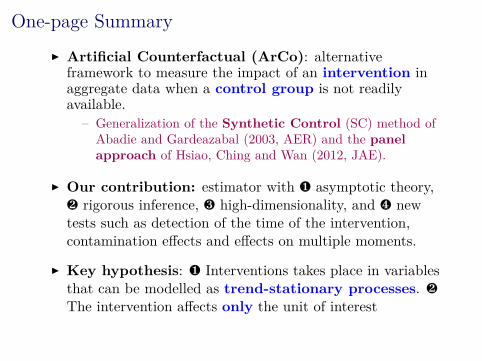
The road map
1. The setup2. The counterfactual estimation3. Estimator properties4. Inference5. Extensions6. Simulations7. Empirical example: Nota Fiscal Paulista8. Research agenda9. Concluding remarks
Setup
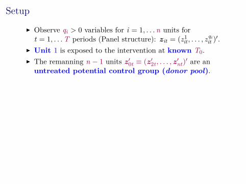
Observe qi > 0 variables for i = 1, . . .n units fort = 1, . . .T periods (Panel structure): z it = (z1it , . . . , z
qiit )
′.
Unit 1 is exposed to the intervention at known T0. The remanning n − 1 units z ′
0t ≡ (z ′2t , . . . , z ′
nt)′ are an
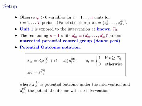
untreated potential control group (donor pool). Potential Outcome notation:
z1t = dtz(1)1t + (1− dt)z(0)
1t ; dt =
1 if t ≥ T0
0 otherwise
z0t = z(0)0t
where z(1)it is potential outcome under the intervention and
z(0)it the potential outcome with no intervention.
Setup
Observe qi > 0 variables for i = 1, . . .n units fort = 1, . . .T periods (Panel structure): z it = (z1it , . . . , z
qiit )
′.
Unit 1 is exposed to the intervention at known T0.
The remanning n − 1 units z ′0t ≡ (z ′
2t , . . . , z ′nt)
′ are anuntreated potential control group (donor pool).
Potential Outcome notation:
z1t = dtz(1)1t + (1− dt)z(0)
1t ; dt =
1 if t ≥ T0
0 otherwise
z0t = z(0)0t
where z(1)it is potential outcome under the intervention and
z(0)it the potential outcome with no intervention.
Setup
Observe qi > 0 variables for i = 1, . . .n units fort = 1, . . .T periods (Panel structure): z it = (z1it , . . . , z
qiit )
′.
Unit 1 is exposed to the intervention at known T0. The remanning n − 1 units z ′
0t ≡ (z ′2t , . . . , z ′
nt)′ are an
untreated potential control group (donor pool).
Potential Outcome notation:
z1t = dtz(1)1t + (1− dt)z(0)
1t ; dt =
1 if t ≥ T0
0 otherwise
z0t = z(0)0t
where z(1)it is potential outcome under the intervention and
z(0)it the potential outcome with no intervention.
Setup
Observe qi > 0 variables for i = 1, . . .n units fort = 1, . . .T periods (Panel structure): z it = (z1it , . . . , z
qiit )
′.
Unit 1 is exposed to the intervention at known T0. The remanning n − 1 units z ′
0t ≡ (z ′2t , . . . , z ′
nt)′ are an
untreated potential control group (donor pool). Potential Outcome notation:
z1t = dtz(1)1t + (1− dt)z(0)
1t ; dt =
1 if t ≥ T0
0 otherwise
z0t = z(0)0t
where z(1)it is potential outcome under the intervention and
z(0)it the potential outcome with no intervention.
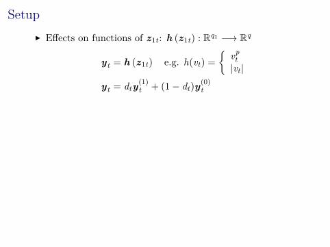
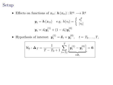
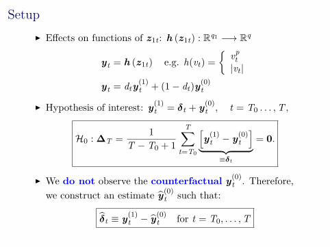
Setup Effects on functions of z1t : h (z1t) : Rq1 −→ Rq
yt = h (z1t) e.g. h(vt) =
vp
t|vt |
yt = dty(1)t + (1− dt)y(0)
t
Hypothesis of interest: y(1)t = δt + y(0)
t , t = T0 . . . ,T ,
H0 : ∆T =1
T − T0 + 1
T∑t=T0
[y(1)
t − y(0)t
]︸ ︷︷ ︸
≡δt
= 0.
We do not observe the counterfactual y(0)t . Therefore,
we construct an estimate y(0)t such that:
δt ≡ y(1)t − y(0)
t for t = T0, . . . ,T
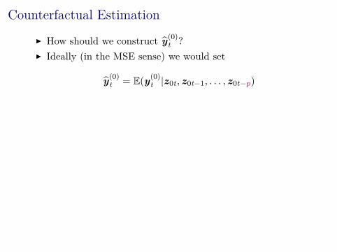
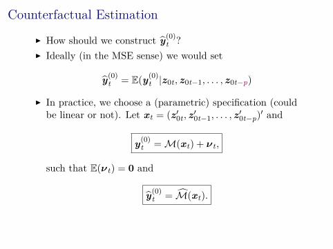
Counterfactual Estimation
How should we construct y(0)t ?
Ideally (in the MSE sense) we would set
y(0)t = E(y(0)
t |z0t , z0t−1, . . . , z0t−p)
In practice, we choose a (parametric) specification (couldbe linear or not). Let xt = (z ′
0t , z ′0t−1, . . . , z ′
0t−p)′ and
y(0)t = M(xt) + νt ,
such that E(νt) = 0 and
y(0)t = M(xt).
ArCo estimator
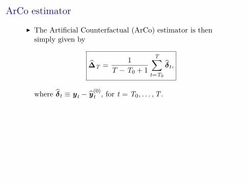
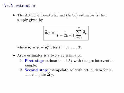
The Artificial Counterfactual (ArCo) estimator is thensimply given by
∆T =1
T − T0 + 1
T∑t=T0
δt ,
where δt ≡ yt − y(0)t , for t = T0, . . . ,T .
ArCo estimator is a two-step estimator:1. First step: estimation of M with the pre-intervention
sample;2. Second step: extrapolate M with actual data for xt
and compute ∆T .
ArCo estimator
The Artificial Counterfactual (ArCo) estimator is thensimply given by
∆T =1
T − T0 + 1
T∑t=T0
δt ,
where δt ≡ yt − y(0)t , for t = T0, . . . ,T .
ArCo estimator is a two-step estimator:1. First step: estimation of M with the pre-intervention
sample;2. Second step: extrapolate M with actual data for xt
and compute ∆T .
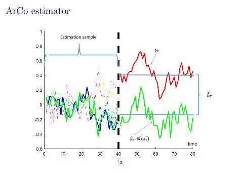
ArCo estimator
𝑦𝑡= 𝑀(𝑥𝑡)
𝑦𝑡
Δ𝑇
Estimation sample

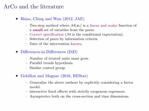
ArCo and the literature
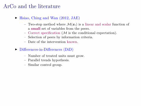
Hsiao, Ching and Wan (2012, JAE)– Two-step method where M(xt) is a linear and scalar function of
a small set of variables from the peers.– Correct specification (M is the conditional expectation).– Selection of peers by information criteria.– Date of the intervention known.
Differences-in-Differences (DiD)– Number of treated units must grow.– Parallel trends hypothesis.– Similar control group.
Gobillon and Magnac (2016, REStat)– Generalize the above authors by explicitly considering a factor
model.– interactive fixed effects with strictly exogenous regressors.– Asymptotics both on the cross-section and time dimensions.
ArCo and the literature
Hsiao, Ching and Wan (2012, JAE)– Two-step method where M(xt) is a linear and scalar function of
a small set of variables from the peers.– Correct specification (M is the conditional expectation).– Selection of peers by information criteria.– Date of the intervention known.
Differences-in-Differences (DiD)– Number of treated units must grow.– Parallel trends hypothesis.– Similar control group.
Gobillon and Magnac (2016, REStat)– Generalize the above authors by explicitly considering a factor
model.– interactive fixed effects with strictly exogenous regressors.– Asymptotics both on the cross-section and time dimensions.

ArCo and the literature
Abadie and Gardeazabal (2003, AER)– Convex combination of peers.– The weights are estimated using time averages of the observed
variables. No time-series dynamics.
Pesaran et al. (2004, JBES); Dees et al. (2007, JAE)– Counterfactual based on variables that belong to the treated
unit. No donor pool.– Their key assumption is that a subset of variables of the treated
unit is invariant to the intervention.
Angrist, Jordà and Kuersteiner (2016, JBES)– Information only on the treated unit and no donor pool is
available.
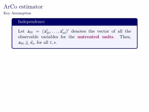
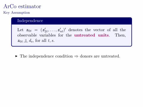
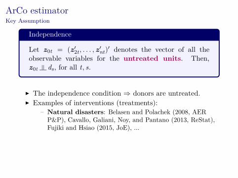
ArCo estimatorKey Assumption
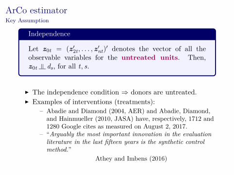
Independence
Let z0t = (z ′2t , . . . , z ′
nt)′ denotes the vector of all the
observable variables for the untreated units. Then,z0t |= ds, for all t, s.
The independence condition ⇒ donors are untreated. Examples of interventions (treatments):
– Natural disasters: Belasen and Polachek (2008, AERP&P), Cavallo, Galiani, Noy, and Pantano (2013, ReStat),Fujiki and Hsiao (2015, JoE), ...
– Region specific policies (laws): Hsiao, Ching, and Wan(2012, JAE), Abadie, Diamond, and Hainmueller (AJPS,2015), Gobillon and Magnac (ReStat, 2016), ...
– New government or political regime: Grier andMaynard (2013, JEBO)
ArCo estimatorKey Assumption
Independence
Let z0t = (z ′2t , . . . , z ′
nt)′ denotes the vector of all the
observable variables for the untreated units. Then,z0t |= ds, for all t, s.
The independence condition ⇒ donors are untreated.
Examples of interventions (treatments):
– Natural disasters: Belasen and Polachek (2008, AERP&P), Cavallo, Galiani, Noy, and Pantano (2013, ReStat),Fujiki and Hsiao (2015, JoE), ...
– Region specific policies (laws): Hsiao, Ching, and Wan(2012, JAE), Abadie, Diamond, and Hainmueller (AJPS,2015), Gobillon and Magnac (ReStat, 2016), ...
– New government or political regime: Grier andMaynard (2013, JEBO)
ArCo estimatorKey Assumption
Independence
Let z0t = (z ′2t , . . . , z ′
nt)′ denotes the vector of all the
observable variables for the untreated units. Then,z0t |= ds, for all t, s.
The independence condition ⇒ donors are untreated. Examples of interventions (treatments):
– Natural disasters: Belasen and Polachek (2008, AERP&P), Cavallo, Galiani, Noy, and Pantano (2013, ReStat),Fujiki and Hsiao (2015, JoE), ...
– Region specific policies (laws): Hsiao, Ching, and Wan(2012, JAE), Abadie, Diamond, and Hainmueller (AJPS,2015), Gobillon and Magnac (ReStat, 2016), ...
– New government or political regime: Grier andMaynard (2013, JEBO)
ArCo estimatorKey Assumption
Independence
Let z0t = (z ′2t , . . . , z ′
nt)′ denotes the vector of all the
observable variables for the untreated units. Then,z0t |= ds, for all t, s.
The independence condition ⇒ donors are untreated.
Examples of interventions (treatments):
– Abadie and Diamond (2004, AER) and Abadie, Diamond,and Hainmueller (2010, JASA) have, respectively, 1712 and1280 Google cites as measured on August 2, 2017.
– “Arguably the most important innovation in the evaluationliterature in the last fifteen years is the synthetic controlmethod.”
Athey and Imbens (2016)
ArCo estimatorKey Assumption
Independence
Let z0t = (z ′2t , . . . , z ′
nt)′ denotes the vector of all the
observable variables for the untreated units. Then,z0t |= ds, for all t, s.
The independence condition ⇒ donors are untreated. Examples of interventions (treatments):
– Abadie and Diamond (2004, AER) and Abadie, Diamond,and Hainmueller (2010, JASA) have, respectively, 1712 and1280 Google cites as measured on August 2, 2017.
– “Arguably the most important innovation in the evaluationliterature in the last fifteen years is the synthetic controlmethod.”
Athey and Imbens (2016)
Counterfactual Estimation
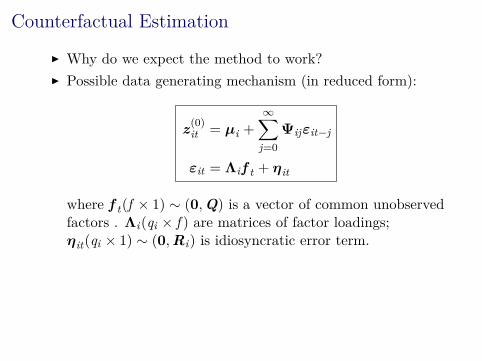
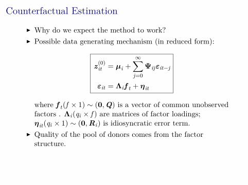
Why do we expect the method to work?
Possible data generating mechanism (in reduced form):
z(0)it = µi +
∞∑j=0
Ψijεit−j
εit = Λif t + ηit
where f t(f × 1) ∼ (0,Q) is a vector of common unobservedfactors . Λi(qi × f ) are matrices of factor loadings;ηit(qi × 1) ∼ (0,Ri) is idiosyncratic error term.
Quality of the pool of donors comes from the factorstructure.
Counterfactual Estimation
Why do we expect the method to work? Possible data generating mechanism (in reduced form):
z(0)it = µi +
∞∑j=0
Ψijεit−j
εit = Λif t + ηit
where f t(f × 1) ∼ (0,Q) is a vector of common unobservedfactors . Λi(qi × f ) are matrices of factor loadings;ηit(qi × 1) ∼ (0,Ri) is idiosyncratic error term.
Quality of the pool of donors comes from the factorstructure.
Counterfactual estimationLeast Absolute Shrinkage and Selection Operator (LASSO)
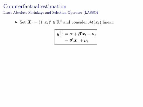
Set X t = (1,xt)′ ∈ Rd and consider M(xt) linear:
y(0)t = α+ β′xt + νt
= θ′X t + νt .
Estimation:
θ = arg min
T0−1∑t=1
(y(0)
t − θ′X t
)2+ ς
d∑j=1
|βj |
. Why LASSO?
– Avoid overfitting.– Large dataset compared to the sample size.– “Automatic” model selection.
Counterfactual estimationLeast Absolute Shrinkage and Selection Operator (LASSO)
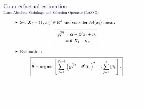
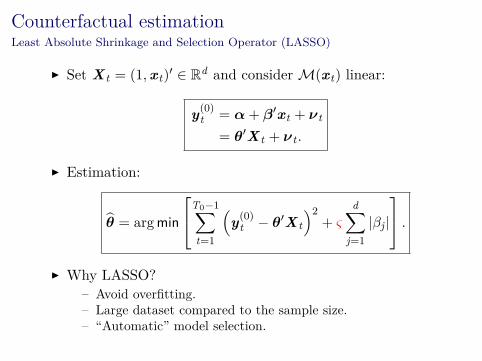
Set X t = (1,xt)′ ∈ Rd and consider M(xt) linear:
y(0)t = α+ β′xt + νt
= θ′X t + νt .
Estimation:
θ = arg min
T0−1∑t=1
(y(0)
t − θ′X t
)2+ ς
d∑j=1
|βj |
.
Why LASSO?– Avoid overfitting.– Large dataset compared to the sample size.– “Automatic” model selection.
Counterfactual estimationLeast Absolute Shrinkage and Selection Operator (LASSO)
Set X t = (1,xt)′ ∈ Rd and consider M(xt) linear:
y(0)t = α+ β′xt + νt
= θ′X t + νt .
Estimation:
θ = arg min
T0−1∑t=1
(y(0)
t − θ′X t
)2+ ς
d∑j=1
|βj |
. Why LASSO?
– Avoid overfitting.– Large dataset compared to the sample size.– “Automatic” model selection.
Counterfactual estimationLASSO – Catalog of hypotheses
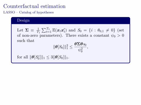
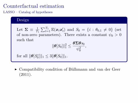
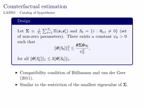
Design
Let Σ ≡ 1T1
∑T1t=1 E(xtx ′
t) and S0 = i : θ0,1 = 0 (setof non-zero parameters). There exists a constant ψ0 > 0such that
∥θ[S0]∥21 ≤θΣθs0ψ20
,
for all ∥θ[Sc0 ]∥1 ≤ 3∥θ[S0]∥1.
Compatibility condition of Bülhmann and van der Geer(2011).
Similar to the restriction of the smallest eigenvalue of Σ. Important for prediction consistency and ℓ1-consistency of
the LASSO.
Counterfactual estimationLASSO – Catalog of hypotheses
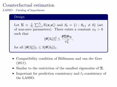
Design
Let Σ ≡ 1T1
∑T1t=1 E(xtx ′
t) and S0 = i : θ0,1 = 0 (setof non-zero parameters). There exists a constant ψ0 > 0such that
∥θ[S0]∥21 ≤θΣθs0ψ20
,
for all ∥θ[Sc0 ]∥1 ≤ 3∥θ[S0]∥1.
Compatibility condition of Bülhmann and van der Geer(2011).
Similar to the restriction of the smallest eigenvalue of Σ.
Important for prediction consistency and ℓ1-consistency ofthe LASSO.
Counterfactual estimationLASSO – Catalog of hypotheses
Design
Let Σ ≡ 1T1
∑T1t=1 E(xtx ′
t) and S0 = i : θ0,1 = 0 (setof non-zero parameters). There exists a constant ψ0 > 0such that
∥θ[S0]∥21 ≤θΣθs0ψ20
,
for all ∥θ[Sc0 ]∥1 ≤ 3∥θ[S0]∥1.
Compatibility condition of Bülhmann and van der Geer(2011).
Similar to the restriction of the smallest eigenvalue of Σ. Important for prediction consistency and ℓ1-consistency of
the LASSO.
Counterfactual estimationLASSO – Catalog of hypotheses
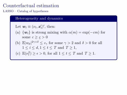
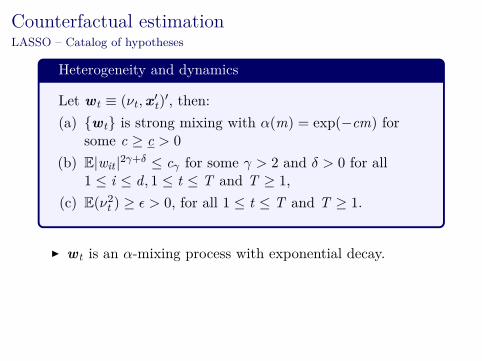
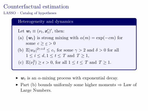
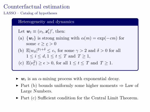
Heterogeneity and dynamics
Let wt ≡ (νt ,x ′t)
′, then:(a) wt is strong mixing with α(m) = exp(−cm) for
some c ≥ c > 0
(b) E|wit |2γ+δ ≤ cγ for some γ > 2 and δ > 0 for all1 ≤ i ≤ d, 1 ≤ t ≤ T and T ≥ 1,
(c) E(ν2t ) ≥ ϵ > 0, for all 1 ≤ t ≤ T and T ≥ 1.
wt is an α-mixing process with exponential decay. Part (b) bounds uniformly some higher moments ⇒ Law of
Large Numbers. Part (c) Sufficient condition for the Central Limit Theorem.
Counterfactual estimationLASSO – Catalog of hypotheses
Heterogeneity and dynamics
Let wt ≡ (νt ,x ′t)
′, then:(a) wt is strong mixing with α(m) = exp(−cm) for
some c ≥ c > 0
(b) E|wit |2γ+δ ≤ cγ for some γ > 2 and δ > 0 for all1 ≤ i ≤ d, 1 ≤ t ≤ T and T ≥ 1,
(c) E(ν2t ) ≥ ϵ > 0, for all 1 ≤ t ≤ T and T ≥ 1.
wt is an α-mixing process with exponential decay.
Part (b) bounds uniformly some higher moments ⇒ Law ofLarge Numbers.
Part (c) Sufficient condition for the Central Limit Theorem.
Counterfactual estimationLASSO – Catalog of hypotheses
Heterogeneity and dynamics
Let wt ≡ (νt ,x ′t)
′, then:(a) wt is strong mixing with α(m) = exp(−cm) for
some c ≥ c > 0
(b) E|wit |2γ+δ ≤ cγ for some γ > 2 and δ > 0 for all1 ≤ i ≤ d, 1 ≤ t ≤ T and T ≥ 1,
(c) E(ν2t ) ≥ ϵ > 0, for all 1 ≤ t ≤ T and T ≥ 1.
wt is an α-mixing process with exponential decay. Part (b) bounds uniformly some higher moments ⇒ Law of
Large Numbers.
Part (c) Sufficient condition for the Central Limit Theorem.
Counterfactual estimationLASSO – Catalog of hypotheses
Heterogeneity and dynamics
Let wt ≡ (νt ,x ′t)
′, then:(a) wt is strong mixing with α(m) = exp(−cm) for
some c ≥ c > 0
(b) E|wit |2γ+δ ≤ cγ for some γ > 2 and δ > 0 for all1 ≤ i ≤ d, 1 ≤ t ≤ T and T ≥ 1,
(c) E(ν2t ) ≥ ϵ > 0, for all 1 ≤ t ≤ T and T ≥ 1.
wt is an α-mixing process with exponential decay. Part (b) bounds uniformly some higher moments ⇒ Law of
Large Numbers. Part (c) Sufficient condition for the Central Limit Theorem.
Counterfactual estimationLASSO – Catalog of hypotheses
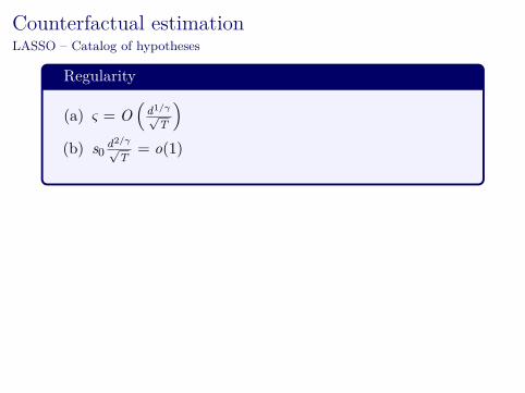
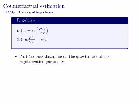
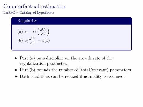
Regularity
(a) ς = O(
d1/γ√
T
)(b) s0 d2/γ
√T = o(1)
Part (a) puts discipline on the growth rate of theregularization parameter.
Part (b) bounds the number of (total/relevant) parameters. Both conditions can be relaxed if normality is assumed.
Counterfactual estimationLASSO – Catalog of hypotheses
Regularity
(a) ς = O(
d1/γ√
T
)(b) s0 d2/γ
√T = o(1)
Part (a) puts discipline on the growth rate of theregularization parameter.
Part (b) bounds the number of (total/relevant) parameters. Both conditions can be relaxed if normality is assumed.

Counterfactual estimationLASSO – Catalog of hypotheses
Regularity
(a) ς = O(
d1/γ√
T
)(b) s0 d2/γ
√T = o(1)
Part (a) puts discipline on the growth rate of theregularization parameter.
Part (b) bounds the number of (total/relevant) parameters.
Both conditions can be relaxed if normality is assumed.
Counterfactual estimationLASSO – Catalog of hypotheses
Regularity
(a) ς = O(
d1/γ√
T
)(b) s0 d2/γ
√T = o(1)
Part (a) puts discipline on the growth rate of theregularization parameter.
Part (b) bounds the number of (total/relevant) parameters. Both conditions can be relaxed if normality is assumed.
Counterfactual estimationLASSO – Results
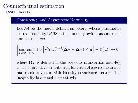
Consistency and Asymptotic Normality
Let M be the model defined as before, whose parametersare estimated by LASSO, then under previous assumptionsand as T → ∞:
supP∈P
supa∈Rq
∣∣∣PP
[√TΩ
−1/2T (∆T −∆T ) ≤ a
]− Φ(a)
∣∣∣ → 0,
where ΩT is defined in the previous proposition and Φ(·)is the cumulative distribution function of a zero-mean nor-mal random vector with identity covariance matrix. Theinequality is defined element-wise.
Counterfactual estimationLASSO – Results
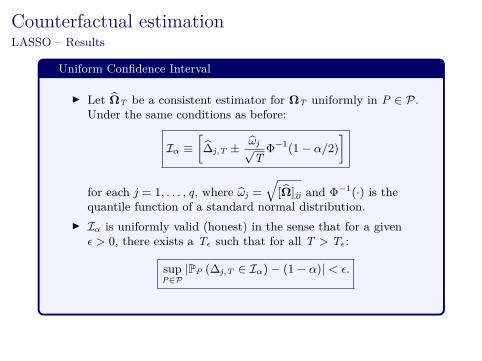
Uniform Confidence Interval
Let ΩT be a consistent estimator for ΩT uniformly in P ∈ P.Under the same conditions as before:
Iα ≡[∆j,T ± ωj√
TΦ−1(1− α/2)
]
for each j = 1, . . . , q, where ωj =
√[Ω]jj and Φ−1(·) is the
quantile function of a standard normal distribution. Iα is uniformly valid (honest) in the sense that for a given
ϵ > 0, there exists a Tϵ such that for all T > Tϵ:
supP∈P
|PP (∆j,T ∈ Iα)− (1− α)| < ϵ.
Counterfactual estimationLASSO – Results
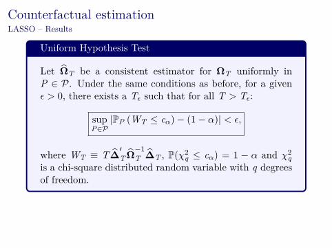
Uniform Hypothesis Test
Let ΩT be a consistent estimator for ΩT uniformly inP ∈ P. Under the same conditions as before, for a givenϵ > 0, there exists a Tϵ such that for all T > Tϵ:
supP∈P
|PP (WT ≤ cα)− (1− α)| < ϵ,
where WT ≡ T∆′T Ω
−1
T ∆T , P(χ2q ≤ cα) = 1 − α and χ2
qis a chi-square distributed random variable with q degreesof freedom.

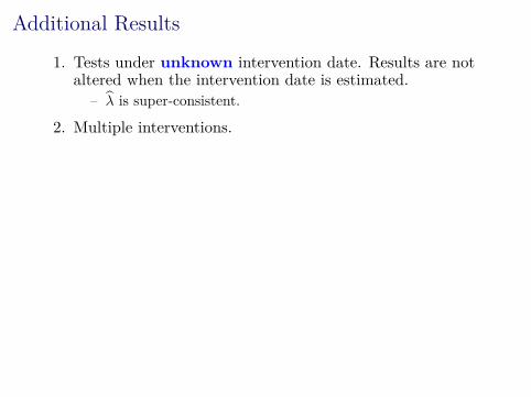
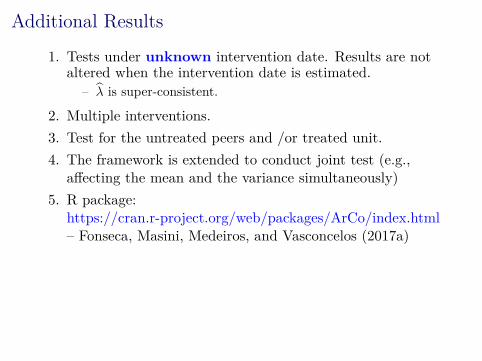
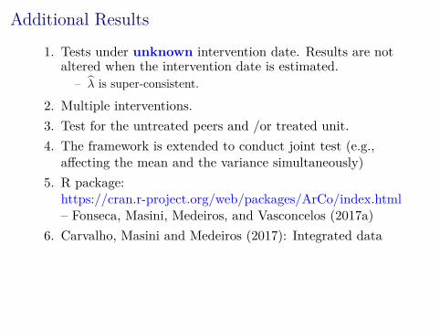
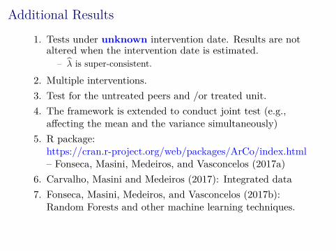
Additional Results
1. Tests under unknown intervention date. Results are notaltered when the intervention date is estimated.
– λ is super-consistent.
2. Multiple interventions.3. Test for the untreated peers and /or treated unit.4. The framework is extended to conduct joint test (e.g.,
affecting the mean and the variance simultaneously)5. R package:
https://cran.r-project.org/web/packages/ArCo/index.html– Fonseca, Masini, Medeiros, and Vasconcelos (2017a)
6. Carvalho, Masini and Medeiros (2017): Integrated data7. Fonseca, Masini, Medeiros, and Vasconcelos (2017b):
Random Forests and other machine learning techniques.
Additional Results
1. Tests under unknown intervention date. Results are notaltered when the intervention date is estimated.
– λ is super-consistent.
2. Multiple interventions.
3. Test for the untreated peers and /or treated unit.4. The framework is extended to conduct joint test (e.g.,
affecting the mean and the variance simultaneously)5. R package:
https://cran.r-project.org/web/packages/ArCo/index.html– Fonseca, Masini, Medeiros, and Vasconcelos (2017a)
6. Carvalho, Masini and Medeiros (2017): Integrated data7. Fonseca, Masini, Medeiros, and Vasconcelos (2017b):
Random Forests and other machine learning techniques.
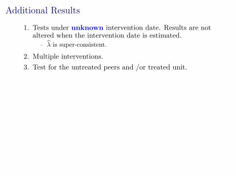
Additional Results
1. Tests under unknown intervention date. Results are notaltered when the intervention date is estimated.
– λ is super-consistent.
2. Multiple interventions.3. Test for the untreated peers and /or treated unit.
4. The framework is extended to conduct joint test (e.g.,affecting the mean and the variance simultaneously)
5. R package:https://cran.r-project.org/web/packages/ArCo/index.html– Fonseca, Masini, Medeiros, and Vasconcelos (2017a)
6. Carvalho, Masini and Medeiros (2017): Integrated data7. Fonseca, Masini, Medeiros, and Vasconcelos (2017b):
Random Forests and other machine learning techniques.
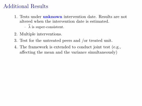
Additional Results
1. Tests under unknown intervention date. Results are notaltered when the intervention date is estimated.
– λ is super-consistent.
2. Multiple interventions.3. Test for the untreated peers and /or treated unit.4. The framework is extended to conduct joint test (e.g.,
affecting the mean and the variance simultaneously)
5. R package:https://cran.r-project.org/web/packages/ArCo/index.html– Fonseca, Masini, Medeiros, and Vasconcelos (2017a)
6. Carvalho, Masini and Medeiros (2017): Integrated data7. Fonseca, Masini, Medeiros, and Vasconcelos (2017b):
Random Forests and other machine learning techniques.
Additional Results
1. Tests under unknown intervention date. Results are notaltered when the intervention date is estimated.
– λ is super-consistent.
2. Multiple interventions.3. Test for the untreated peers and /or treated unit.4. The framework is extended to conduct joint test (e.g.,
affecting the mean and the variance simultaneously)5. R package:
https://cran.r-project.org/web/packages/ArCo/index.html– Fonseca, Masini, Medeiros, and Vasconcelos (2017a)
6. Carvalho, Masini and Medeiros (2017): Integrated data7. Fonseca, Masini, Medeiros, and Vasconcelos (2017b):
Random Forests and other machine learning techniques.
Additional Results
1. Tests under unknown intervention date. Results are notaltered when the intervention date is estimated.
– λ is super-consistent.
2. Multiple interventions.3. Test for the untreated peers and /or treated unit.4. The framework is extended to conduct joint test (e.g.,
affecting the mean and the variance simultaneously)5. R package:
https://cran.r-project.org/web/packages/ArCo/index.html– Fonseca, Masini, Medeiros, and Vasconcelos (2017a)
6. Carvalho, Masini and Medeiros (2017): Integrated data
7. Fonseca, Masini, Medeiros, and Vasconcelos (2017b):Random Forests and other machine learning techniques.
Additional Results
1. Tests under unknown intervention date. Results are notaltered when the intervention date is estimated.
– λ is super-consistent.
2. Multiple interventions.3. Test for the untreated peers and /or treated unit.4. The framework is extended to conduct joint test (e.g.,
affecting the mean and the variance simultaneously)5. R package:
https://cran.r-project.org/web/packages/ArCo/index.html– Fonseca, Masini, Medeiros, and Vasconcelos (2017a)
6. Carvalho, Masini and Medeiros (2017): Integrated data7. Fonseca, Masini, Medeiros, and Vasconcelos (2017b):
Random Forests and other machine learning techniques.
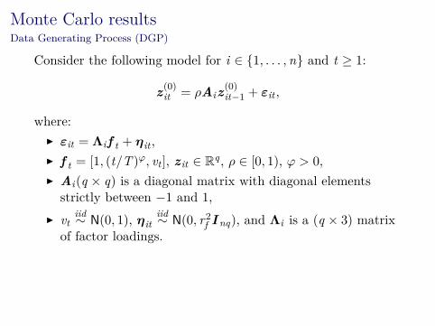
Monte Carlo resultsData Generating Process (DGP)
Consider the following model for i ∈ 1, . . . ,n and t ≥ 1:
z(0)it = ρAiz(0)
it−1 + εit ,
where: εit = Λif t + ηit , f t = [1, (t/T )φ, vt ], z it ∈ Rq , ρ ∈ [0, 1), φ > 0, Ai(q × q) is a diagonal matrix with diagonal elements
strictly between −1 and 1, vt
iid∼ N(0, 1), ηitiid∼ N(0, r2f I nq), and Λi is a (q × 3) matrix
of factor loadings.
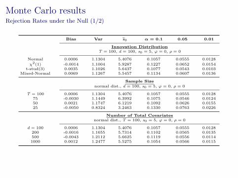
Monte Carlo resultsRejection Rates under the Null (1/2)
Bias Var s0 α = 0.1 0.05 0.01
Innovation DistributionT = 100, d = 100, s0 = 5, φ = 0, ρ = 0
Normal 0.0006 1.1304 5.4076 0.1057 0.0555 0.0128χ2(1) -0.0014 1.1004 5.9287 0.1227 0.0652 0.0154
t-stud(3) 0.0035 1.1026 5.6437 0.1077 0.0543 0.0103Mixed-Normal 0.0069 1.1267 5.5457 0.1134 0.0607 0.0136
Sample Sizenormal dist., d = 100, s0 = 5, φ = 0, ρ = 0
T = 100 0.0006 1.1304 5.4076 0.1057 0.0555 0.012875 -0.0030 1.1449 6.3992 0.1075 0.0546 0.012450 0.0021 1.1747 6.1219 0.1092 0.0626 0.015525 -0.0050 0.8324 3.2463 0.1330 0.0763 0.0226
Number of Total Covariatesnormal dist., T = 100, s0 = 5, φ = 0, ρ = 0
d = 100 0.0006 1.1304 5.4076 0.1057 0.0555 0.0128200 -0.0016 1.1655 5.7314 0.1102 0.0565 0.0135500 -0.0043 1.2112 5.6625 0.1119 0.0556 0.01141000 0.0012 1.2477 5.5275 0.1054 0.0566 0.0115
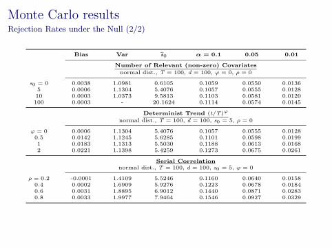
Monte Carlo resultsRejection Rates under the Null (2/2)
Bias Var s0 α = 0.1 0.05 0.01
Number of Relevant (non-zero) Covariatesnormal dist., T = 100, d = 100, φ = 0, ρ = 0
s0 = 0 0.0038 1.0981 0.6105 0.1059 0.0550 0.01365 0.0006 1.1304 5.4076 0.1057 0.0555 0.012810 0.0003 1.0373 9.5813 0.1103 0.0581 0.0120100 0.0003 - 20.1624 0.1114 0.0574 0.0145
Determinist Trend (t/T)φ
normal dist., T = 100, d = 100, s0 = 5, ρ = 0
φ = 0 0.0006 1.1304 5.4076 0.1057 0.0555 0.01280.5 0.0142 1.1245 5.6285 0.1101 0.0598 0.01991 0.0183 1.1313 5.5030 0.1188 0.0613 0.01682 0.0221 1.1398 5.4259 0.1273 0.0675 0.0261
Serial Correlationnormal dist., T = 100, d = 100, s0 = 5, φ = 0
ρ = 0.2 -0.0001 1.4109 5.5246 0.1160 0.0640 0.01580.4 0.0002 1.6909 5.9276 0.1223 0.0678 0.01840.6 0.0031 1.8895 6.9012 0.1440 0.0871 0.02830.8 0.0033 1.9977 7.9464 0.1546 0.0927 0.0329
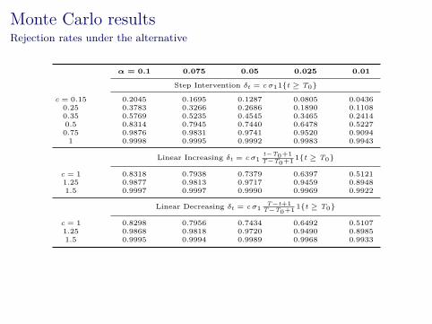
Monte Carlo resultsRejection rates under the alternative
α = 0.1 0.075 0.05 0.025 0.01
Step Intervention δt = c σ11t ≥ T0
c = 0.15 0.2045 0.1695 0.1287 0.0805 0.04360.25 0.3783 0.3266 0.2686 0.1890 0.11080.35 0.5769 0.5235 0.4545 0.3465 0.24140.5 0.8314 0.7945 0.7440 0.6478 0.52270.75 0.9876 0.9831 0.9741 0.9520 0.9094
1 0.9998 0.9995 0.9992 0.9983 0.9943
Linear Increasing δt = c σ1t−T0+1T−T0+1
1t ≥ T0
c = 1 0.8318 0.7938 0.7379 0.6397 0.51211.25 0.9877 0.9813 0.9717 0.9459 0.89481.5 0.9997 0.9997 0.9990 0.9969 0.9922
Linear Decreasing δt = c σ1T−t+1
T−T0+11t ≥ T0
c = 1 0.8298 0.7956 0.7434 0.6492 0.51071.25 0.9868 0.9818 0.9720 0.9490 0.89851.5 0.9995 0.9994 0.9989 0.9968 0.9933
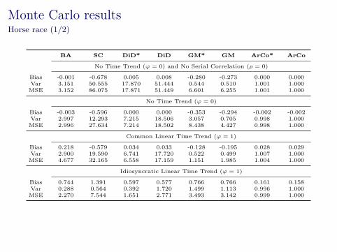
Monte Carlo resultsHorse race (1/2)
BA SC DiD* DiD GM* GM ArCo* ArCo
No Time Trend (φ = 0) and No Serial Correlation (ρ = 0)
Bias -0.001 -0.678 0.005 0.008 -0.280 -0.273 0.000 0.000Var 3.151 50.555 17.870 51.444 0.544 0.510 1.001 1.000
MSE 3.152 86.075 17.871 51.449 6.601 6.255 1.001 1.000
No Time Trend (φ = 0)
Bias -0.003 -0.596 0.000 0.000 -0.353 -0.294 -0.002 -0.002Var 2.997 12.293 7.215 18.506 3.057 0.705 0.998 1.000
MSE 2.996 27.634 7.214 18.502 8.438 4.427 0.998 1.000
Common Linear Time Trend (φ = 1)
Bias 0.218 -0.579 0.034 0.033 -0.128 -0.195 0.028 0.029Var 2.900 19.590 6.741 17.720 0.522 0.499 1.007 1.000
MSE 4.677 32.165 6.558 17.159 1.151 1.985 1.004 1.000
Idiosyncratic Linear Time Trend (φ = 1)
Bias 0.744 1.391 0.597 0.577 0.766 0.766 0.161 0.158Var 0.288 0.564 0.392 1.720 1.499 1.113 0.996 1.000
MSE 2.270 7.544 1.651 2.771 3.493 3.142 0.999 1.000
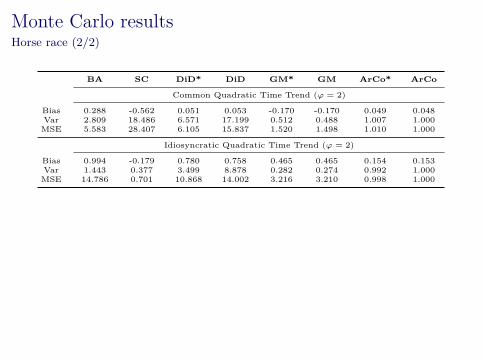
Monte Carlo resultsHorse race (2/2)
BA SC DiD* DiD GM* GM ArCo* ArCo
Common Quadratic Time Trend (φ = 2)
Bias 0.288 -0.562 0.051 0.053 -0.170 -0.170 0.049 0.048Var 2.809 18.486 6.571 17.199 0.512 0.488 1.007 1.000
MSE 5.583 28.407 6.105 15.837 1.520 1.498 1.010 1.000
Idiosyncratic Quadratic Time Trend (φ = 2)
Bias 0.994 -0.179 0.780 0.758 0.465 0.465 0.154 0.153Var 1.443 0.377 3.499 8.878 0.282 0.274 0.992 1.000
MSE 14.786 0.701 10.868 14.002 3.216 3.210 0.998 1.000
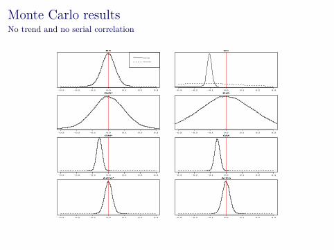
Monte Carlo resultsNo trend and no serial correlation
−0.3 −0.2 −0.1 0.0 0.1 0.2 0.3
BA
N = 10000 Bandwidth = 0.005884
Kernel
Normal
−0.3 −0.2 −0.1 0.0 0.1 0.2 0.3
SC
N = 10000 Bandwidth = 0.002148
Densi
ty
−0.3 −0.2 −0.1 0.0 0.1 0.2 0.3
DiD*
N = 10000 Bandwidth = 0.01388
−0.3 −0.2 −0.1 0.0 0.1 0.2 0.3
DiD
N = 10000 Bandwidth = 0.02359
Densi
ty
−0.3 −0.2 −0.1 0.0 0.1 0.2 0.3
GM*
N = 10000 Bandwidth = 0.002445
−0.3 −0.2 −0.1 0.0 0.1 0.2 0.3
GM
N = 10000 Bandwidth = 0.002358
Densi
ty
−0.3 −0.2 −0.1 0.0 0.1 0.2 0.3
ArCo*
−0.3 −0.2 −0.1 0.0 0.1 0.2 0.3
ArCo
Densi
ty
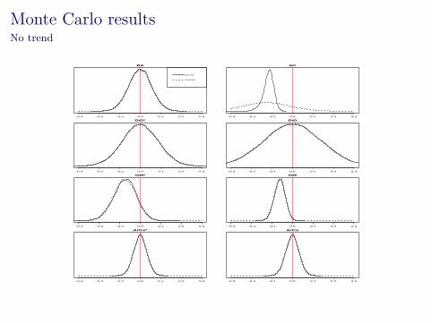
Monte Carlo resultsNo trend
−0.3 −0.2 −0.1 0.0 0.1 0.2 0.3
BA
N = 10000 Bandwidth = 0.007846
Kernel
Normal
−0.3 −0.2 −0.1 0.0 0.1 0.2 0.3
SC
N = 10000 Bandwidth = 0.003405
Densi
ty
−0.3 −0.2 −0.1 0.0 0.1 0.2 0.3
DiD*
N = 10000 Bandwidth = 0.01239
−0.3 −0.2 −0.1 0.0 0.1 0.2 0.3
DiD
N = 10000 Bandwidth = 0.01985
Densi
ty
−0.3 −0.2 −0.1 0.0 0.1 0.2 0.3
GM*
N = 10000 Bandwidth = 0.007959
−0.3 −0.2 −0.1 0.0 0.1 0.2 0.3
GM
N = 10000 Bandwidth = 0.003859
Densi
ty
−0.3 −0.2 −0.1 0.0 0.1 0.2 0.3
ArCo*
−0.3 −0.2 −0.1 0.0 0.1 0.2 0.3
ArCo
Densi
ty
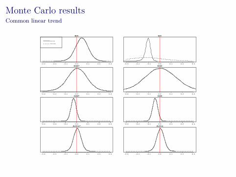
Monte Carlo resultsCommon linear trend
−0.3 −0.2 −0.1 0.0 0.1 0.2 0.3
BA
N = 10000 Bandwidth = 0.00805
Kernel
Normal
−0.3 −0.2 −0.1 0.0 0.1 0.2 0.3
SC
N = 10000 Bandwidth = 0.003059
Densi
ty
−0.3 −0.2 −0.1 0.0 0.1 0.2 0.3
DiD*
N = 10000 Bandwidth = 0.01217
−0.3 −0.2 −0.1 0.0 0.1 0.2 0.3
DiD
N = 10000 Bandwidth = 0.0198
Densi
ty
−0.3 −0.2 −0.1 0.0 0.1 0.2 0.3
GM*
N = 10000 Bandwidth = 0.003377
−0.3 −0.2 −0.1 0.0 0.1 0.2 0.3
GM
N = 10000 Bandwidth = 0.003315
Densi
ty
−0.3 −0.2 −0.1 0.0 0.1 0.2 0.3
ArCo*
−0.3 −0.2 −0.1 0.0 0.1 0.2 0.3
ArCo
Densi
ty
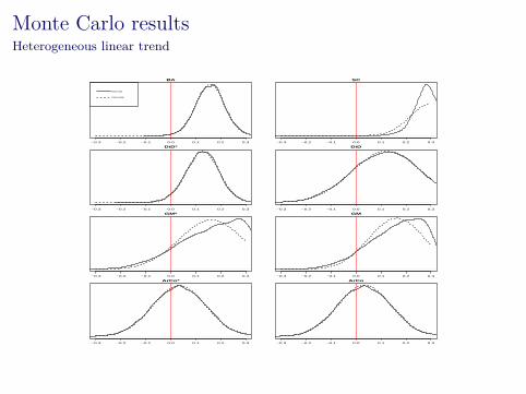
Monte Carlo resultsHeterogeneous linear trend
−0.3 −0.2 −0.1 0.0 0.1 0.2 0.3
BA
N = 10000 Bandwidth = 0.008106
Kernel
Normal
−0.3 −0.2 −0.1 0.0 0.1 0.2 0.3
SC
N = 10000 Bandwidth = 0.007246
Densi
ty
−0.3 −0.2 −0.1 0.0 0.1 0.2 0.3
DiD*
N = 10000 Bandwidth = 0.009353
−0.3 −0.2 −0.1 0.0 0.1 0.2 0.3
DiD
N = 10000 Bandwidth = 0.01988
Densi
ty
−0.3 −0.2 −0.1 0.0 0.1 0.2 0.3
GM*
N = 10000 Bandwidth = 0.01856
−0.3 −0.2 −0.1 0.0 0.1 0.2 0.3
GM
N = 10000 Bandwidth = 0.01599
Densi
ty
−0.3 −0.2 −0.1 0.0 0.1 0.2 0.3
ArCo*
−0.3 −0.2 −0.1 0.0 0.1 0.2 0.3
ArCo
Densi
ty
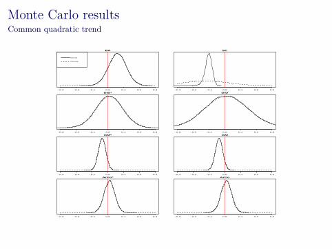
Monte Carlo resultsCommon quadratic trend
−0.3 −0.2 −0.1 0.0 0.1 0.2 0.3
BA
N = 10000 Bandwidth = 0.008015
Kernel
Normal
−0.3 −0.2 −0.1 0.0 0.1 0.2 0.3
SC
N = 10000 Bandwidth = 0.003058
Densi
ty
−0.3 −0.2 −0.1 0.0 0.1 0.2 0.3
DiD*
N = 10000 Bandwidth = 0.01217
−0.3 −0.2 −0.1 0.0 0.1 0.2 0.3
DiD
N = 10000 Bandwidth = 0.01988
Densi
ty
−0.3 −0.2 −0.1 0.0 0.1 0.2 0.3
GM*
N = 10000 Bandwidth = 0.003422
−0.3 −0.2 −0.1 0.0 0.1 0.2 0.3
GM
N = 10000 Bandwidth = 0.003337
Densi
ty
−0.3 −0.2 −0.1 0.0 0.1 0.2 0.3
ArCo*
−0.3 −0.2 −0.1 0.0 0.1 0.2 0.3
ArCo
Densi
ty

Monte Carlo resultsHeterogeneous quadratic trend
−0.3 −0.2 −0.1 0.0 0.1 0.2 0.3
BA
N = 10000 Bandwidth = 0.00799
Kernel
Normal
−0.3 −0.2 −0.1 0.0 0.1 0.2 0.3
SC
N = 10000 Bandwidth = 0.002572
Densi
ty
−0.3 −0.2 −0.1 0.0 0.1 0.2 0.3
DiD*
N = 10000 Bandwidth = 0.01228
−0.3 −0.2 −0.1 0.0 0.1 0.2 0.3
DiD
N = 10000 Bandwidth = 0.01982
Densi
ty
−0.3 −0.2 −0.1 0.0 0.1 0.2 0.3
GM*
N = 10000 Bandwidth = 0.003487
−0.3 −0.2 −0.1 0.0 0.1 0.2 0.3
GM
N = 10000 Bandwidth = 0.003469
Densi
ty
−0.3 −0.2 −0.1 0.0 0.1 0.2 0.3
ArCo*
−0.3 −0.2 −0.1 0.0 0.1 0.2 0.3
ArCo
Densi
ty

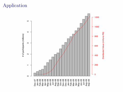
Application
In October 2007, the state government of São Paulo inBrazil implemented a anti tax evasion scheme called NotaFiscal Paulista (NFP).
The NFP consists of a tax rebate from a state tax namedICMS (tax on circulation of products and services).
Incentive to the consumer to ask for sales receipts. Additionally, the registered sales receipts give the consumer
the right to participate in monthly lotteries promoted bythe government.

Application
In October 2007, the state government of São Paulo inBrazil implemented a anti tax evasion scheme called NotaFiscal Paulista (NFP).
The NFP consists of a tax rebate from a state tax namedICMS (tax on circulation of products and services).
Incentive to the consumer to ask for sales receipts.
Additionally, the registered sales receipts give the consumerthe right to participate in monthly lotteries promoted bythe government.

Application
In October 2007, the state government of São Paulo inBrazil implemented a anti tax evasion scheme called NotaFiscal Paulista (NFP).
The NFP consists of a tax rebate from a state tax namedICMS (tax on circulation of products and services).
Incentive to the consumer to ask for sales receipts. Additionally, the registered sales receipts give the consumer
the right to participate in monthly lotteries promoted bythe government.

Application Under the premisses that:
1. a certain degree of tax evasion was occurring before theintervention,
2. the sellers has some degree of market power and3. the penalty for tax-evasion is large enough to alter the seller
behaviour,one is expected to see an upwards movements in prices dueto an increase in marginal cost.
Hence, we would like to investigate whether the NFP hadan impact on consumer prices in São Paulo.

Application
The NFP was not implemented throughout the sectors inthe economy at once.
The first sector were restaurants, followed by bakeries, barand other food service retailers.
The sample then consists of monthly inflation (food outsidehome) index for 10 metropolitan areas including São Paulofrom Jan-05 to Sep-09.
Application
Dec−0
7Ja
n−08
Feb−
08M
ar−0
8Ap
r−08
May−0
8Ju
n−08
Jul−
08Au
g−08
Sep−
08O
ct−0
8N
ov−0
8D
ec−0
8Ja
n−09
Feb−
09M
ar−0
9Ap
r−09
May−0
9Ju
n−09
Jul−
09Au
g−09
Sep−
09
# of
par
ticip
ants
(milli
ons)
01
23
45
Dis
tribu
ted
Valu
e (m
illion
s R
$)
0
200
400
600
800
1000
1200
Application
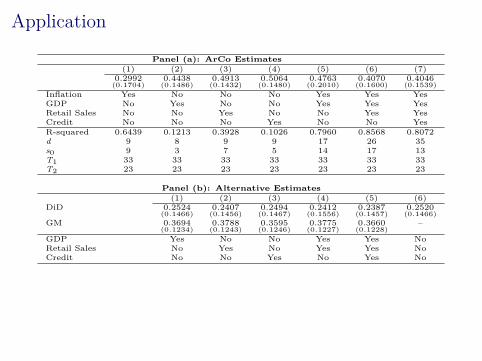
Panel (a): ArCo Estimates(1) (2) (3) (4) (5) (6) (7)
0.2992(0.1704)
0.4438(0.1486)
0.4913(0.1432)
0.5064(0.1480)
0.4763(0.2010)
0.4070(0.1600)
0.4046(0.1539)
Inflation Yes No No No Yes Yes YesGDP No Yes No No Yes Yes YesRetail Sales No No Yes No No Yes YesCredit No No No Yes No No YesR-squared 0.6439 0.1213 0.3928 0.1026 0.7960 0.8568 0.8072d 9 8 9 9 17 26 35s0 9 3 7 5 14 17 13T1 33 33 33 33 33 33 33T2 23 23 23 23 23 23 23
Panel (b): Alternative Estimates(1) (2) (3) (4) (5) (6)
DiD 0.2524(0.1466)
0.2407(0.1456)
0.2494(0.1467)
0.2412(0.1556)
0.2387(0.1457)
0.2520(0.1466)
GM 0.3694(0.1234)
0.3788(0.1243)
0.3595(0.1246)
0.3775(0.1227)
0.3660(0.1228)
–
GDP Yes No No Yes Yes NoRetail Sales No Yes No Yes Yes NoCredit No No Yes No Yes No
Application
Jan-05 Jan-06 Jan-07 Jan-08 Jan-09
-0.5
0
0.5
1
1.5
2
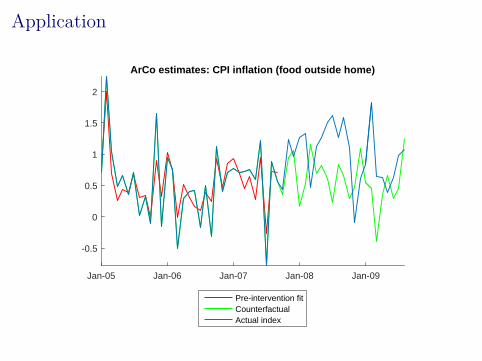
ArCo estimates: CPI inflation (food outside home)
Pre-intervention fitCounterfactualActual index
Application
Jan-05 Jan-06 Jan-07 Jan-08 Jan-09
1.05
1.1
1.15
1.2
1.25
1.3
1.35
1.4
1.45
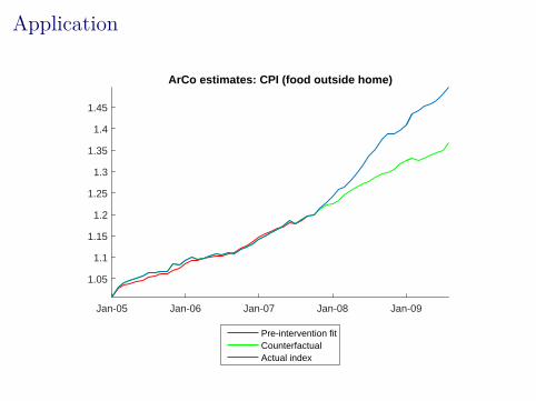
ArCo estimates: CPI (food outside home)
Pre-intervention fitCounterfactualActual index
Concluding remarks
Important to note that the ArCo is more than just anotherstructural break estimator.
By controlling for common shocks that might haveoccurred in all units after the intervention, it provides aeffective methodology to isolate the effect of theintervention of interest.
Providing compelling evidence for the causality of thestructural break observed in the unit of interest
It is almost a model-free methodology. It implies nostructure in the stationary process (no # of lags to bedetermined nor # MA terms)