Appendix E – Modeling Report - USGS E – Modeling Report ... FLOW module and the Delft3D-Wave...
120
785 Appendix E – Modeling Report This appendix contains the modeling report submitted by John Brocatus as part of his M.S. Thesis in Coastal Engineering at Delft University of Technology. The report is part of the cooperation between Deltares and United States Geological Survey (USGS), and was funded by the USGS through a grant from BEACON. A summary of this report is presented in Chapter 9 (Numerical Modeling Sediment Budget Analysis for the Santa Barbara Littoral Cell using Delft3D) of the main report.
-
Upload
truongdien -
Category
Documents
-
view
215 -
download
2
Transcript of Appendix E – Modeling Report - USGS E – Modeling Report ... FLOW module and the Delft3D-Wave...
785
Appendix E – Modeling Report
This appendix contains the modeling report submitted by John Brocatus as part of his M.S.
Thesis in Coastal Engineering at Delft University of Technology. The report is part of the cooperation
between Deltares and United States Geological Survey (USGS), and was funded by the USGS through a
grant from BEACON. A summary of this report is presented in Chapter 9 (Numerical Modeling
Sediment Budget Analysis for the Santa Barbara Littoral Cell using Delft3D) of the main report.

Sediment Budget Analysis of the Santa Barbara Littoral Cell A study to identify and quantify the pathways of sediment transport

Prepared for:
USGS
Sediment Budget Analysis of the Santa Barbara Littoral Cell A study to identify and quantify the pathways of sediment transport
J. Brocatus Supervising Committee: Prof.dr.ir. M.J.F. Stive Delft University of TechnologyDr.ir. E.P.L. Elias Deltares Ir. D.J.R. Walstra Deltares Dr. P.L. Barnard US Geological Survey Dr.ir. L.H. Holthuijsen Delft University of Technology
Report
October 2008
© Deltares, 2008


Sediment Budget Analysis of the Santa Barbara Littoral Cell October 2008
Deltares Preface
Preface
This M.Sc. thesis is written to complete my master in Coastal Engineering at the faculty of Civil Engineering and Geosciences of Delft University of Technology. The thesis is part of the cooperation between Deltares and United States Geological Survey (USGS), within the framework of many research USGS is doing in the Santa Barbara region. Many people have contributed in different ways to the realisation of this thesis. First of all I would like to thank my graduation committee, prof. dr. ir. M.J.F. Stive (Delft University of Technology), dr. ir. E.P.L. Elias (Deltares / USGS), ir. D.J.R. Walstra (Deltares), dr. P.L. Barnard (USGS) and dr.ir. L.H. Holthuijsen (Delft University of Technology) for their effort. Special thanks goes out to Christoph Brière for his help using Delft3D. Furthermore I would like to thank Deltares and the USGS for the facilities they offered in the Netherlands and in Santa Cruz. I hope you will enjoy reading this report. John Brocatus Delft, October 2008

Sediment Budget Analysis of the Santa Barbara Littoral Cell October 2008
Deltares Summary
Summary
The Santa Barbara Littoral Cell is one of the longest cells in southern California. At Point Conception, the coastline abruptly changes from a north/south orientation to an east/west orientation. There is a gradual change in the type of coastline from west to east. From Point Conception up to almost 15 miles west of the city of Goleta, the coastline primarily consists of bluffs. Then, while less exposed to the northwestern swell, the coastline consists of bluffs altering with primarily narrow beaches from Goleta up to the city of Ventura. From there, up to the Mugu Submarine Canyons, the Ventura River and the Santa Clara River have created a large alluvial plane. The majority of beaches within the Santa Barbara and Ventura County study area are narrow and ephemeral. The beaches near the cities of Goleta and Carpinteria and the Ventura River mouth are facing coastal retreat due to erosion. At present, most erosion problems within the region are thought to be induced by human interference into the coastal system. Besides the damming and canalization of rivers, also the armouring of the coastline and the disruption of the longshore sediment transport by the construction of breakwaters and jetties has reduced the sediment supply necessary to preserve the beaches. The aim of this study is to identify and quantify the pathways of sediment transport within the Santa Barbara Littoral Cell. A Delft3D numerical model is used to model the hydro- and morphodynamics. Input filtering techniques are used to simplify relevant hydrodynamic input conditions to reduce the run time for the simulation. With respect to the wave climate, this implies that the model is only forced with the wave conditions that contribute most to the longshore sediment transport. The entire wave climate is schematised into a morphological representative wave climate that consists of ten wave conditions. Four wave conditions originate from the south/south-east whereas the remaining conditions originate from the west. The relative root mean square error between the total sediment transport and the sediment transport resulting from the reduced set of wave conditions is 5.62%. Originally, these waves are present during 30 days a year, but in order to resemble the total transport, their total probability of occurrence is increased to 61.97 % or 226 days a year. The schematisation of the tide is based on a reduction of the tidal constituents. The original set, the astronomical tide, consists of 37 constituents. The reduced tide (so-called morphological tide) consists of three constituents that dominate the flow and sediment pattern. The flow pattern of the morphological tide has a strong correlation with the flow pattern of the astronomical tide, although current magnitudes are being underestimated by approximately 50%. Consequently, the same is observed for the tide induced sediment transport. The almost negligible contribution of the tide to the sediment transport with respect to the contribution of the waves justifies the use of the morphological tide. The model results show a high correlation with the data. The abrupt counter clockwise rotation of the coastline at the western side of Ellwood Beach locally increases the residual velocities. Halfway Ellwood Beach, the coastline bends back in seaward direction and the velocities decrease up to Devereux Slough. Consequently, erosion occurs at the western part of Ellwood Beach, whereas the eastern side of the beach in front of the Devereux Slough accretes. At Isla Vista Beach, a similar pattern is observed. The lack of sediment being transported around Campus Point however prevents the beaches of UCSB and the part of Goleta Beach west to Goleta Slough to accrete. East of Goleta slough, the residual current increases and is dominated by western swell, resulting in an eroding trend of Goleta Beach.

October 2008 Sediment Budget Analysis of the Santa Barbara Littoral Cell
ii Deltares
There is a long-term trend of erosion at the City of Carpinteria Beach and accretion at the eastern side of Carpinteria state Beach. The revetment along the coastline directly upcoast of the City of Carpinteria Beach and along Sandyland, maintains the erosion at the City of Carpinteria Beach. While the revetment prevents erosion at Sandyland and fixates Sandy Point, rotation of the coastline (i.e. reducing the angle of wave approach) is restricted to the beaches in front of Carpinteria. The fixation of Sandyland prevents the adaptation of the coastline to the prevailing wave condition and maintains the relative large angle of wave approach of western swells. The erosion within the Santa Barbara Littoral Cell is not associated with a significant reduction of sediment supply from the upstream rivers by human alterations, but primarily caused by the prevailing wave climate and the local orientation of the coastline. The beaches that face erosion or accretion locally have strong gradients in the sediment transport. These gradients are the primary source of erosion and accretion. Increasing the amount of sediment supply (e.g. by dam removal or beach nourishments), will not have effect on the transport gradients and will therefore not solve the erosion problems.

Sediment Budget Analysis of the Santa Barbara Littoral Cell October 2008
Deltares i
Contents
List of Figures
1 Introduction.......................................................................................................1 1.1 What is littoral drift? ................................................................................1 1.2 What are littoral cells? ............................................................................3 1.3 Santa Barbara Littoral Cell......................................................................4
1.3.1 General overview........................................................................4 1.3.2 Hydrodynamics...........................................................................5 1.3.3 Sediment sources.......................................................................5 1.3.4 Sediment characteristics ............................................................5 1.3.5 Littoral drift rates.........................................................................5
2 Problem definition and objectives...................................................................5 2.1 Problem analysis ....................................................................................5 2.2 Research objectives ...............................................................................5 2.3 Research approach and Outline .............................................................5
3 Model description .............................................................................................5 3.1 Delft3D-Online (2DH) modelling approach .............................................5 3.2 Computational grids................................................................................5 3.3 Bathymetric schematisation....................................................................5 3.4 Parameter settings..................................................................................5
3.4.1 Parameter settings Delf3D-FLOW..............................................5 3.4.2 Parameter settings Delft3D-WAVE.............................................5
4 Schematisation of boundary conditions.........................................................5 4.1 The concept of input reduction ...............................................................5 4.2 Schematisation of the wave climate........................................................5
4.2.1 Introduction.................................................................................5 4.2.2 Validation of the SWAN-model ...................................................5 4.2.3 Application of a wave schematisation in the Santa Barbara
Channel ......................................................................................5 4.2.4 Remarks .....................................................................................5
4.3 Schematisation of tidal currents..............................................................5 4.3.1 Introduction.................................................................................5 4.3.2 Application of a morphological tide in the Santa Barbara
Channel ......................................................................................5 5 Sensitivity analysis...........................................................................................5
5.1 Introduction.............................................................................................5 5.2 Reference simulation ..............................................................................5 5.3 Scaling of the grain size..........................................................................5

October 2008 Sediment Budget Analysis of the Santa Barbara Littoral Cell
ii Deltares
5.4 Scaling of the current-related suspended and bed load..........................5 5.5 Scaling of the wave-related suspended and bed load.............................5 5.6 River discharge .......................................................................................5
5.6.1 Average annual river discharge ..................................................5 5.6.2 Flood river discharge ..................................................................5
6 Evaluation of the final simulation ....................................................................5 6.1 Model setup ............................................................................................5 6.2 Analysis of the residual current ...............................................................5
6.2.1 Tidal current................................................................................5 6.2.2 Residual Current.........................................................................5
6.3 Analysis of the littoral drift .......................................................................5 7 Conclusions and recommendations................................................................5
7.1 Conclusions ............................................................................................5 7.2 Recommendations ..................................................................................5
8 References.........................................................................................................5
Appendices A Governing equations Delft3D FLOW and WAVE ............................................5 B Conceptual description Opti-Routine..............................................................5 C Tables.................................................................................................................5 D Wenthworth-Krumbein scale of sediment size...............................................5 E Sensitivity analysis: summary .........................................................................5 F Figures ...............................................................................................................5
Sediment Budget Analysis of the Santa Barbara Littoral Cell October 2008
Deltares iii
List of Figures
Figure 1-1 Development of a longshore current due to oblique incoming waves. This current is, together with the turbulence of the breaking waves, the driving force for sediment movement along the shore. The net movement of sediment in the direction of the littoral current is referred to as the littoral drift. ...................................................................................1
Figure 1-2 Relation between longshore sediment transport (Sx) and angle of wave approach (φ0)..........................................................................................2
Figure 1-3 The littoral cell concept. The sediment transport within the cell is bounded, indicating that no sediment will be transported through the cell boundaries. .............................................................................................3
Figure 1-4 Map of North America. Detailed window: at the west coast, in the State of California, the Santa Barbara Channel is located. The east/west orientation of the coastline provides some shelter to swell that predominantly come from the north-west direction. ................................4
Figure 1-5 Tidal data at NOAA tide gauge station 9411340 at Santa Barbara Harbor. The tide has a diurnal character with a strong semi-diurnal distortion. Water levels are related to the Mean Lower Low Water (MLLW), which is 0,029 m below NAVD..........................................................................5
Figure 1-6 Circulation pattern in the Southern California Bight From: http://seis.natsci.csulb.edu/bperry/scbweb/circulation ............................5
Figure 1-7 Location of wave buoys. Offshore wave buoys: 46063 and 46069 (NDBC). Nearshore wave buoys: 46216 and 46217 (CDIP). ................................5
Figure 1-8 Daily river runoff for the Santa Clara River and the Ventura River in which the episodic character is evident Santa Clara River discharge information is obtained from USGS river gauging station 11114000 (Santa Clara River at Montalvo);Ventura River discharge information is obtained from USGS river gauging station 11118500.............................5
Figure 3-1 The Delft3D software package. The heart of the framework is the FLOW-module....................................................................................................5
Figure 3-2 Modelling scheme of the Delft3D-Online Modelling approach. The Delft3D-FLOW module and the Delft3D-Wave module are coupled to account for both the effects of waves on currents and the effect of flow on waves. ..5
Figure 3-3 Computational grids: wave grid (upper panel) and flow grid (lower panel). The flow grid is also used as a nested wave grid to ensure a high grid resolution in the surf zone.......................................................................5
Figure 3-4 Open boundary conditions. At the seaward boundary (A-B), the water level is prescribed. At the lateral boundaries (A-A’ and B-B’) the water level gradient as a function of time is imposed (so-called Neumann boundaries).............................................................................................5
Figure 4-1 Time series of the significant wave height during a 12 hour storm period (red) at December 8th 2007 as registered by station 46063....................5
October 2008 Sediment Budget Analysis of the Santa Barbara Littoral Cell
ii Deltares
Figure 4-2 Validation of the SWAN-model, based on the significant wave height, wave period and wave direction. Station 46063 is located close to the western model boundary, station 46216 is located in the Santa Barbara Channel (near Goleta) and station 46217 is located near Anacapa Passage. ......5
Figure 4-3 Overview of the 27 predefined transects. ......................................................5 Figure 4-4 Upper panel: comparison of the non-validated littoral drift rates for the entire
(green) and the reduced (yellow) wave climate. The relative root mean square error is 5.62%. Other panels: Individual sediment transport contribution for each wave condition within the schematised wave climate.....................................................................................................5
Figure 4-5 Timeseries of the morphological tide (red) and the astronomical tide (blue). 5 Figure 4-6 Residual current pattern for the astronomical tide (upper panel) and the
morphological tide (lower panel). ............................................................5 Figure 4-7 Residual sediment transport pattern for the astronomical tide (upper panel)
and the morphological tide (lower panel). ...............................................5 Figure 4-8 Annual net sediment transport for a morphological (red) and an
astronomical tide (blue)...........................................................................5 Figure 5-1 Transects through which the littoral drift rates are determined. Transect 12
and 14 represent the dredging volumes at the Santa Barbara and the Ventura Harbor, respectively...................................................................5
Figure 5-2 Influence of the grain size (D50) on littoral drift rates .....................................5 Figure 5-3 Influence of the current related suspended and bed load parameter
(sus/bed) on littoral drift rates..................................................................5 Figure 5-4 Effect of susw/bedw on the littoral drift ..........................................................5 Figure 5-5 Influence of the wave related suspended and bed load parameter
(susw/bedw) on littoral drift rates ............................................................5 Figure 5-6 Distribution of the river sediment concentration at the last time step of the
simulation................................................................................................5 Figure 5-7 Influence of the average annual Santa Clara and Ventura River discharge
on the littoral drift rates............................................................................5 Figure 5-8 Influence of the mean annual Santa Clara and Ventura River flood
discharge on the littoral drift rates ...........................................................5 Figure 6-1 Grid resolution in the Santa Barbara region for both the coarse and refined
grid. .........................................................................................................5 Figure 6-2 Coarse (black) and refined grid (red).............................................................5 Figure 6-3 Circulation pattern in the Southern California Bight
http://seis.natsci.csulb.edu/bperry/scbweb/.............................................5 Figure 6-4 Tidal current pattern for (a) flood, (b) ebb and (c) residual. ...........................5 Figure 6-5 Tidal sediment transport pattern for (a) flood, (b) ebb and (c) residual..........5 Figure 6-6 Subdivision of the model domain. Sections 3, 5 and 7 (indicated in red)
represent the focus sites. ........................................................................5 Figure 6-7 Impression of the energy dissipation near the focus sites for a southern
(upper panel) and a western (lower panel) swell.....................................5

Sediment Budget Analysis of the Santa Barbara Littoral Cell October 2008
Deltares iii
Figure 6-8 Significant wave height and its trajectory near Goleta Platform for wave condition 88 (left panel) and wave condition 62 (right panel). ................5
Figure 6-9 Residual current pattern for (a) section 1, (b) section 2, (c) section 3 and (d) section 4. ................................................................................................5
Figure 6-10 Significant wave height and its trajectory near Santa Barbara Platform for wave condition 62 (upper panel) and wave condition 88 (lower panel)...5
Figure 6-11 Trajectory for (red) wave condition 62 (dir=170°N) and (black) wave condition 88 ( dir =278°N). ......................................................................5
Figure 6-12 Residual current pattern for section 5. ........................................................5 Figure 6-13 Residual current pattern for section 6. ........................................................5 Figure 6-14 Significant wave height and its trajectory near Ventura Harbor for wave
condition 88 (left panel) and wave condition 62 (right panel). ................5 Figure 6-15 Residual current pattern for section 7. ........................................................5 Figure 6-16 Residual sediment transport vectors for the Santa Barbara Channel. ........5 Figure 6-17 Littoral drift rates for the Santa Barbara Channel........................................5 Figure 6-18 Individual sediment transport contribution by each wave condition within
the morphological representative wave climate (colored lines) to the total annual sediment transport (yellow bars). ........................................5
Figure 6-19 Littoral drift gradients causing erosion (red) and accretion (blue) at sandy parts of the coastline...............................................................................5
Figure 6-20 Mean total transport over the entire simulation period for the Goleta Region (upper panel) and Carpinteria Region (lower panel)...................5
Figure 6-21 Mean total transport over the entire simulation period for Ventura Region .5

Sediment Budget Analysis of the Santa Barbara Littoral Cell October 2008
Deltares 1
1 Introduction
1.1 What is littoral drift?
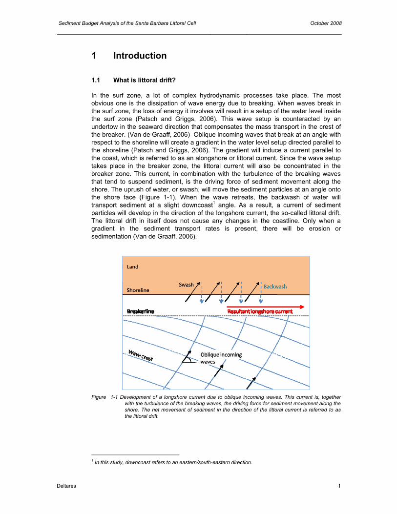
In the surf zone, a lot of complex hydrodynamic processes take place. The most obvious one is the dissipation of wave energy due to breaking. When waves break in the surf zone, the loss of energy it involves will result in a setup of the water level inside the surf zone (Patsch and Griggs, 2006). This wave setup is counteracted by an undertow in the seaward direction that compensates the mass transport in the crest of the breaker. (Van de Graaff, 2006) Oblique incoming waves that break at an angle with respect to the shoreline will create a gradient in the water level setup directed parallel to the shoreline (Patsch and Griggs, 2006). The gradient will induce a current parallel to the coast, which is referred to as an alongshore or littoral current. Since the wave setup takes place in the breaker zone, the littoral current will also be concentrated in the breaker zone. This current, in combination with the turbulence of the breaking waves that tend to suspend sediment, is the driving force of sediment movement along the shore. The uprush of water, or swash, will move the sediment particles at an angle onto the shore face (Figure 1-1). When the wave retreats, the backwash of water will transport sediment at a slight downcoast1 angle. As a result, a current of sediment particles will develop in the direction of the longshore current, the so-called littoral drift. The littoral drift in itself does not cause any changes in the coastline. Only when a gradient in the sediment transport rates is present, there will be erosion or sedimentation (Van de Graaff, 2006).
Figure 1-1 Development of a longshore current due to oblique incoming waves. This current is, together
with the turbulence of the breaking waves, the driving force for sediment movement along the shore. The net movement of sediment in the direction of the littoral current is referred to as the littoral drift.
1 In this study, downcoast refers to an eastern/south-eastern direction.

October 2008 Sediment Budget Analysis of the Santa Barbara Littoral Cell
2 Deltares
The effect of the angle of wave incidence on the littoral drift can be examined by the relationship between the longshore sediment transport through the breaker zone (S) and the deep water wave angle (φ0). In the CERC-formula (1.1), which is an empirical prediction of alongshore sediment transport, the relation between the sediment transport and the angle of wave approach is expressed as;
52
1 1 0sin(2 )bS H Kα ϕ= (1.1)
Figure 1-2 Relation between longshore sediment transport (Sx) and angle of wave approach (φ0)
The sinusoidal character of the deepwater wave angle indicates that the maximum longshore sediment transport occurs for waves that approach with an angle of 45° with respect to the shore normal (Van de Graaff, 2006). For wave angles larger than 45°, the longshore sediment transport (Sx) decreases again. The (S, φ)-diagram illustrates this relationship (Figure 1-2). The direction of the littoral drift might be directed to the right (looking seaward) during part of the year and to the left during the remainder of the year. If the left and right transports are denoted QlL and QlR, respectively, with QlR being positive and QlL being negative, then, according to Inman and Masters (1991), the net annual transport QlNET is defined as: lNET lR lLQ Q Q= + (1.2) This implies that the net longshore sediment transport rate is directed to the right and positive if QlR> QlL and directed to the left and negative if QlR< |QlL|. The gross annual longshore transport QlGROSS is defined as the sum of the magnitudes of the littoral transport, irrespective of the direction:
lGROSS lR lLQ Q Q= + (1.3)
These two different definitions of sediment movement have their own specific applications. For example, the gross sediment transport can give insight in the shoaling rates in navigation channels, whereas the net sediment transport is useful to determine the long term erosion/sedimentation rates along the coast.

Sediment Budget Analysis of the Santa Barbara Littoral Cell October 2008
Deltares 3
1.2 What are littoral cells?
The Californian coastline can be divided into a number of segments in which the littoral sediment transport is said to be bounded (Patsch and Griggs, 2006). Each segment has its own sediment sources and sinks, and little or no littoral sediment transport takes place between adjacent segments (Figure 1-3). These segments, which are referred to as littoral cells, start ideally with a section of coast along which no or little sediment transport occurs. The sediment sources within a littoral cell can be either natural or artificial. River and stream runoff is the main component of natural sediment input for the Californian coastal system. Other natural input components, like bluff erosion and cross-shore exchange of sediment, are also significant but contribute mostly to a lesser extent. Typical forms of artificial sediment supply are beach nourishment and sand bypassing.
Figure 1-3 The littoral cell concept. The sediment transport within the cell is bounded, indicating that no
sediment will be transported through the cell boundaries.
At the end of the littoral cell, sediment is permanently lost from the system. In California, this is often caused by the presence of submarine canyons. These canyons trap the littoral drift by depositing the sediment in the deepest basins in which it can never find its way back to the shore. Also an abrupt change in the direction of the coastline can result in a permanent loss of littoral sediment. In that case, most sediment will, instead of being transported around the point at which the coast changes direction, be transported to the offshore.

October 2008 Sediment Budget Analysis of the Santa Barbara Littoral Cell
4 Deltares
1.3 Santa Barbara Littoral Cell
1.3.1 General overview
One of the longest cells in southern California is the Santa Barbara Littoral Cell (SBLC). The mouth of the Santa Maria River is currently used as the northern boundary of this cell. Originally, Habel and Armstrong (1978) defined the northern boundary of the Santa Barbara Littoral Cell south of the Santa Ynez River. Patsch (2004) concluded that the boundary needed to be extended to include the Santa Maria River Mouth (Patsch and Riggs, 2007). From there, the cell stretches 230 kilometres towards the submarine canyon at Point Mugu. According to Patsch and Griggs (2007), this canyon function as an almost complete trap for the littoral drift and can therefore be seen as the downdrift boundary of the cell. The 40-kilometre wide Santa Barbara Channel separates the so-called Northern Channel Islands from the mainland (Figure 1-4). These islands used to be a single landmass known as Santa Rosae, but ongoing erosion divided the landmass into four islands: Santa Rosa, Santa Cruz, San Miguel and Anacapa Island. Tectonic plate movement along the San Andreas Fault caused the Santa Barbara channel and the Santa Ynez Mountain Range to become aligned east to west (Henson and Usner, 1996). As a result, the coastline changes from a north/south orientation to an east/west orientation at Point Conception. This, together with the position of the Northern Channel Islands, result in a wave climate in the Santa Barbara Channel that is less energetic than along most parts of the Californian coastline. The east/west orientation shelters the coastline from swell that predominantly comes from the west/north-western direction, while the Northern Channel Islands provide some shelter to the less frequently occurring southern swell.
Figure 1-4 Map of North America. Detailed window: at the west coast, in the State of California, the Santa Barbara Channel is located. The east/west orientation of the coastline provides some shelter to swell that predominantly come from the north-west direction.
Pt. Conception GoletaSanta Barbara
Carpinteria
Santa Barbara Channel
Northern Channel Islands
Ventura River
Santa Clara River
Mugu Submarine Canyon
Sediment Budget Analysis of the Santa Barbara Littoral Cell October 2008
Deltares 5
From Point Conception up to almost 15 miles west of the city of Goleta, the coastline primarily consists of bluffs. Between the cities of Goleta and Ventura, bluffs alternating with primarily narrow beaches dominate. Southeast of Ventura, up to the Mugu Submarine Canyon, the Ventura and Santa Clara River have created an alluvial plane. As a result, the nearshore seabed is relatively shallow and the beaches are wide in the Santa Clara region due to the massive sediment supply. 1.3.2 Hydrodynamics
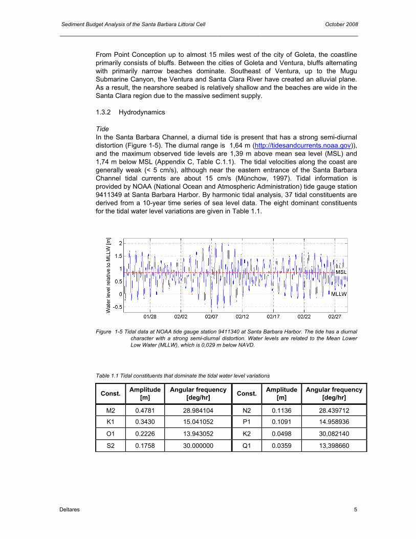
Tide In the Santa Barbara Channel, a diurnal tide is present that has a strong semi-diurnal distortion (Figure 1-5). The diurnal range is 1,64 m (http://tidesandcurrents.noaa.gov)), and the maximum observed tide levels are 1,39 m above mean sea level (MSL) and 1,74 m below MSL (Appendix C, Table C.1.1). The tidal velocities along the coast are generally weak (< 5 cm/s), although near the eastern entrance of the Santa Barbara Channel tidal currents are about 15 cm/s (Münchow, 1997). Tidal information is provided by NOAA (National Ocean and Atmospheric Administration) tide gauge station 9411349 at Santa Barbara Harbor. By harmonic tidal analysis, 37 tidal constituents are derived from a 10-year time series of sea level data. The eight dominant constituents for the tidal water level variations are given in Table 1.1.
Figure 1-5 Tidal data at NOAA tide gauge station 9411340 at Santa Barbara Harbor. The tide has a diurnal
character with a strong semi-diurnal distortion. Water levels are related to the Mean Lower Low Water (MLLW), which is 0,029 m below NAVD.
Table 1.1 Tidal constituents that dominate the tidal water level variations
Const. Amplitude [m]
Angular frequency [deg/hr] Const. Amplitude
[m] Angular frequency
[deg/hr]
M2 0.4781 28.984104 N2 0.1136 28.439712
K1 0.3430 15.041052 P1 0.1091 14.958936
O1 0.2226 13.943052 K2 0.0498 30,082140
S2 0.1758 30.000000 Q1 0.0359 13,398660
October 2008 Sediment Budget Analysis of the Santa Barbara Littoral Cell
6 Deltares
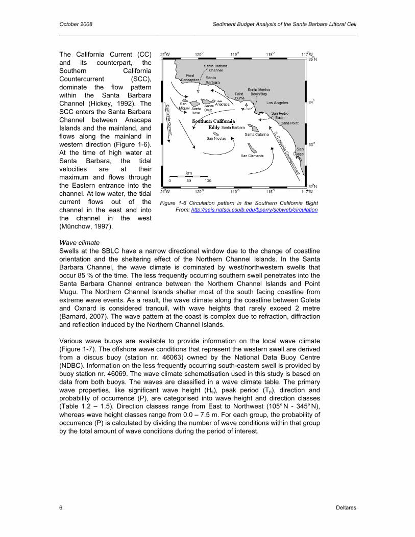
The California Current (CC) and its counterpart, the Southern California Countercurrent (SCC), dominate the flow pattern within the Santa Barbara Channel (Hickey, 1992). The SCC enters the Santa Barbara Channel between Anacapa Islands and the mainland, and flows along the mainland in western direction (Figure 1-6). At the time of high water at Santa Barbara, the tidal velocities are at their maximum and flows through the Eastern entrance into the channel. At low water, the tidal current flows out of the channel in the east and into the channel in the west (Münchow, 1997). Wave climate Swells at the SBLC have a narrow directional window due to the change of coastline orientation and the sheltering effect of the Northern Channel Islands. In the Santa Barbara Channel, the wave climate is dominated by west/northwestern swells that occur 85 % of the time. The less frequently occurring southern swell penetrates into the Santa Barbara Channel entrance between the Northern Channel Islands and Point Mugu. The Northern Channel Islands shelter most of the south facing coastline from extreme wave events. As a result, the wave climate along the coastline between Goleta and Oxnard is considered tranquil, with wave heights that rarely exceed 2 metre (Barnard, 2007). The wave pattern at the coast is complex due to refraction, diffraction and reflection induced by the Northern Channel Islands. Various wave buoys are available to provide information on the local wave climate (Figure 1-7). The offshore wave conditions that represent the western swell are derived from a discus buoy (station nr. 46063) owned by the National Data Buoy Centre (NDBC). Information on the less frequently occurring south-eastern swell is provided by buoy station nr. 46069. The wave climate schematisation used in this study is based on data from both buoys. The waves are classified in a wave climate table. The primary wave properties, like significant wave height (Hs), peak period (Tp), direction and probability of occurrence (P), are categorised into wave height and direction classes (Table 1.2 – 1.5). Direction classes range from East to Northwest (105°N - 345°N), whereas wave height classes range from 0.0 – 7.5 m. For each group, the probability of occurrence (P) is calculated by dividing the number of wave conditions within that group by the total amount of wave conditions during the period of interest.
Figure 1-6 Circulation pattern in the Southern California Bight From: http://seis.natsci.csulb.edu/bperry/scbweb/circulation

Sediment Budget Analysis of the Santa Barbara Littoral Cell October 2008
Deltares 7
Figure 1-7 Location of wave buoys. Offshore wave buoys: 46063 and 46069 (NDBC). Nearshore wave
buoys: 46216 and 46217 (CDIP).
About 75% of all waves within the dataset originate from the west/north-west (270°N - 315°N). Waves from this direction have wave heights ranging from 0.5 – 7.4 m, although waves higher than 5.0 m rarely occur (Table 1.20. The peak period is about 10 seconds for wave heights up to 3.0 m, but increases up to 16 seconds or more for wave heights larger than 5.0 m. No waves come from the North (335°N or more) due to the sheltering effect of Point Conception. The south/south-eastern swell direction ranges from 135°N - 195°N and contributes only 12% to the total dataset. The wave heights are, with a peak value of 4.4 m, lower than swells originating from the west/north-west. The peak periods are relatively higher for south/south-eastern swells (~15.0 – 18.5 sec) than for west/north-western swells (~10.0 – 18.0 sec).

October 2008 Sediment Budget Analysis of the Santa Barbara Littoral Cell
8 Deltares
Table 1.2 Wave climate table. Significant wave height (m)of the different wave conditions.
105 135 150 165 180 195 225 240 255 270 285 300 315 330135 150 165 180 195 225 240 255 270 285 300 315 330 345
1,30 1,29 1,29 1,29 1,28 1,24 1,26 1,20 1,27 1,28 1,30 1,30 1,32 1,35
1,65 1,77 1,69 1,67 1,67 1,69 1,70 1,70 1,74 1,74 1,77 1,77 1,79 1,76
2,07 2,15 2,21 2,21 2,16 2,21 2,24 2,24 2,23 2,23 2,25 2,24 2,23 2,25
0,00 0,00 0,00 2,65 0,00 0,00 2,71 2,62 2,72 2,72 2,74 2,71 2,73 2,77
0,00 3,02 3,42 3,36 0,00 0,00 0,00 0,00 3,22 3,25 3,24 3,23 3,25 3,27
0,00 0,00 3,76 3,75 3,95 3,67 3,69 3,75 3,69 3,72 3,74 3,69 3,71 3,67
0,00 0,00 4,11 4,19 0,00 0,00 0,00 0,00 0,00 4,21 4,23 4,22 4,24 4,29
0,00 0,00 0,00 0,00 0,0 0,00 0,00 0,00 4,69 4,72 4,71 4,73 4,74 0,00
0,00 0,00 0,00 0,00 0,0 0,00 0,00 0,00 0,00 5,21 5,29 5,28 0,00 0,00
0,00 0,00 0,00 0,00 0,0 0,00 0,00 0,00 0,00 5,71 5,74 5,81 0,00 0,00
0,00 0,00 0,00 0,00 0,0 0,00 0,00 0,00 0,00 6,19 6,19 6,18 0,00 0,00
0,00 0,00 0,00 0,00 0,00 0,00 0,00 0,00 0,00 6,61 6,61 6,78 0,00 0,00
0,00 0,00 0,00 0,00 0,00 0,00 0,00 0,00 0,00 7,18 7,27 7,08 0,00 0,00
6,50 - 7,007,00 - 7,50
0,00 - 1,50 1,50 - 2,002,00 - 2,502,50 - 3,003,00 - 3,503,50 - 4,00
4,50 - 5,005,00 - 5,505,50 - 6,006,00 - 6,50
Mean wave height (m)
Wave heightWave direction sector (degrees w .r.t. North)
4,00 - 4,50
Hs (m)
Table 1.3 Wave climate table. Peak wave period (sec) for each wave condition
105 135 150 165 180 195 225 240 255 270 285 300 315 330135 150 165 180 195 225 240 255 270 285 300 315 330 345
15,4 15,4 15,4 15,1 14,9 15,0 14,4 12,7 12,6 12,3 11,1 10,1 10,3 8,9
17,0 15,0 15,3 15,8 15,7 15,6 14,8 13,8 13,6 12,2 10,2 10,1 10,4 10,8
15,2 15,5 15,8 15,4 15,9 15,3 15,5 14,3 14,0 12,8 10,3 10,1 10,8 11,3
0,0 0,0 0,0 15,8 0,0 0,0 13,8 14,5 14,2 13,3 11,1 10,9 11,6 13,4
0,0 14,8 17,4 18,7 0,0 0,0 0,0 0,0 12,0 13,9 12,5 12,4 11,5 12,2
0,0 0,0 18,6 18,5 18,5 19,1 17,4 16,0 7,1 14,2 13,1 12,6 11,3 10,8
0,0 0,0 18,2 17,4 0,0 0,0 0,0 0,0 0,0 13,7 13,2 13,4 11,7 9,1
0,0 0,0 0,0 0,0 0,0 0,0 0,0 0,0 17,4 14,5 13,7 12,1 17,4 0,0
0,0 0,0 0,0 0,0 0,0 0,0 0,0 0,0 0,0 16,0 13,2 12,2 0,0 0,0
0,0 0,0 0,0 0,0 0,0 0,0 0,0 0,0 0,0 15,5 12,8 11,9 0,0 0,0
0,0 0,0 0,0 0,0 0,0 0,0 0,0 0,0 0,0 16,3 13,0 13,0 0,0 0,0
0,0 0,0 0,0 0,0 0,0 0,0 0,0 0,0 0,0 18,2 12,1 13,9 0,0 0,0
0,0 0,0 0,0 0,0 0,0 0,0 0,0 0,0 0,0 18,0 16,1 14,1 0,0 0,0
1,50 - 2,00
4,50 - 5,004,00 - 4,503,50 - 4,003,00 - 3,502,50 - 3,002,00 - 2,50
Peak wave period (s)
0,00 - 1,50
7,00 - 7,506,50 - 7,006,00 - 6,505,50 - 6,005,00 - 5,50
Wave direction sector (degrees w .r.t. North)Wave height
Hs (m)
Table 1.4 Wave climate table. Mean wave direction (deg) of the different wave conditions.
105 135 150 165 180 195 225 240 255 270 285 300 315 330135 150 165 180 195 225 240 255 270 285 300 315 330 345131 146 160 174 188 206 232 248 264 279 293 307 320 334
125 143 158 173 188 206 233 248 265 279 293 306 321 333
126 143 160 174 187 207 237 249 265 280 294 306 321 333
0 0 0 176 0 0 234 251 265 280 294 306 322 334
0 140 153 173 0 0 0 0 266 280 294 306 322 334
0 0 158 170 187 217 239 255 267 280 294 306 320 333
0 0 161 174 0 0 0 0 0 282 295 306 320 332
0 0 0 0 0 0 0 0 270 282 294 305 318 0
0 0 0 0 0 0 0 0 0 280 294 305 0 0
0 0 0 0 0 0 0 0 0 278 295 304 0 0
0 0 0 0 0 0 0 0 0 278 295 304 0 0
0 0 0 0 0 0 0 0 0 282 288 304 0 0
0 0 0 0 0 0 0 0 0 283 293 307 0 0
5,00 - 5,505,50 - 6,006,00 - 6,506,50 - 7,007,00 - 7,50
2,00 - 2,502,50 - 3,003,00 - 3,503,50 - 4,004,00 - 4,504,50 - 5,00
0,00 - 1,50 1,50 - 2,00
Mean wave direction (degrees)
Wave direction sector (degrees w .r.t. North)Wave height
Hs (m)
Sediment Budget Analysis of the Santa Barbara Littoral Cell October 2008
Deltares 9
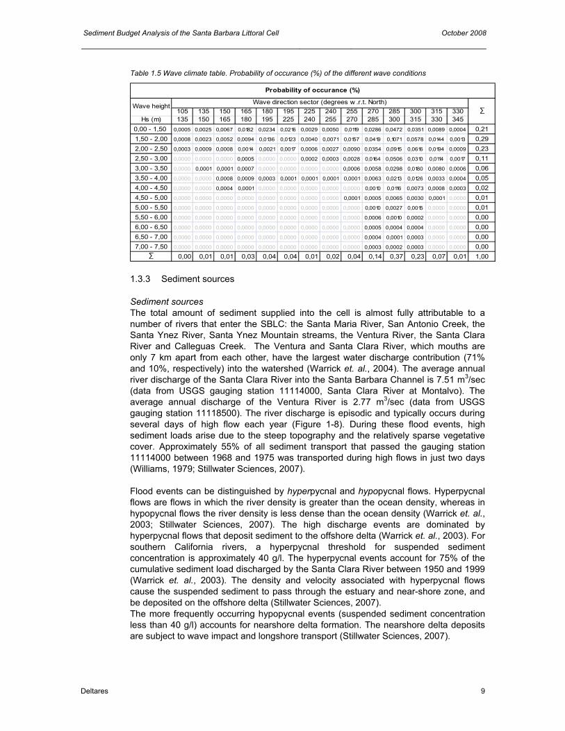
Table 1.5 Wave climate table. Probability of occurance (%) of the different wave conditions
105 135 150 165 180 195 225 240 255 270 285 300 315 330135 150 165 180 195 225 240 255 270 285 300 315 330 345
0,0005 0,0025 0,0067 0,0182 0,0234 0,0216 0,0029 0,0050 0,0119 0,0286 0,0472 0,0351 0,0089 0,0004
0,0008 0,0023 0,0052 0,0094 0,0136 0,0123 0,0040 0,0071 0,0157 0,0419 0,1071 0,0578 0,0144 0,0013
0,0003 0,0009 0,0008 0,0014 0,0021 0,0017 0,0006 0,0027 0,0090 0,0354 0,0915 0,0616 0,0194 0,0009
0,0000 0,0000 0,0000 0,0005 0,0000 0,0000 0,0002 0,0003 0,0028 0,0164 0,0506 0,0310 0,0114 0,0017
0,0000 0,0001 0,0001 0,0007 0,0000 0,0000 0,0000 0,0000 0,0006 0,0058 0,0298 0,0180 0,0080 0,0006
0,0000 0,0000 0,0008 0,0009 0,0003 0,0001 0,0001 0,0001 0,0001 0,0063 0,0213 0,0126 0,0033 0,0004
0,0000 0,0000 0,0004 0,0001 0,0000 0,0000 0,0000 0,0000 0,0000 0,0010 0,0116 0,0073 0,0008 0,0003
0,0000 0,0000 0,0000 0,0000 0,0000 0,0000 0,0000 0,0000 0,0001 0,0005 0,0065 0,0030 0,0001 0,0000
0,0000 0,0000 0,0000 0,0000 0,0000 0,0000 0,0000 0,0000 0,0000 0,0010 0,0027 0,0015 0,0000 0,0000
0,0000 0,0000 0,0000 0,0000 0,0000 0,0000 0,0000 0,0000 0,0000 0,0006 0,0010 0,0002 0,0000 0,0000
0,0000 0,0000 0,0000 0,0000 0,0000 0,0000 0,0000 0,0000 0,0000 0,0005 0,0004 0,0004 0,0000 0,0000
0,0000 0,0000 0,0000 0,0000 0,0000 0,0000 0,0000 0,0000 0,0000 0,0004 0,0001 0,0003 0,0000 0,0000
0,0000 0,0000 0,0000 0,0000 0,0000 0,0000 0,0000 0,0000 0,0000 0,0003 0,0002 0,0003 0,0000 0,0000
0,00 0,01 0,01 0,03 0,04 0,04 0,01 0,02 0,04 0,14 0,37 0,23 0,07 0,01
6,50 - 7,007,00 - 7,50
3,50 - 4,004,00 - 4,504,50 - 5,005,00 - 5,505,50 - 6,006,00 - 6,50
0,00 - 1,50
Probability of occurance (%)
1,00
Wave height
∑
∑Wave direction sector (degrees w .r.t. North)
0,210,290,230,110,060,050,020,010,010,00
Hs (m)
1,50 - 2,002,00 - 2,502,50 - 3,003,00 - 3,50
0,000,000,00
1.3.3 Sediment sources
Sediment sources The total amount of sediment supplied into the cell is almost fully attributable to a number of rivers that enter the SBLC: the Santa Maria River, San Antonio Creek, the Santa Ynez River, Santa Ynez Mountain streams, the Ventura River, the Santa Clara River and Calleguas Creek. The Ventura and Santa Clara River, which mouths are only 7 km apart from each other, have the largest water discharge contribution (71% and 10%, respectively) into the watershed (Warrick et. al., 2004). The average annual river discharge of the Santa Clara River into the Santa Barbara Channel is 7.51 m3/sec (data from USGS gauging station 11114000, Santa Clara River at Montalvo). The average annual discharge of the Ventura River is 2.77 m3/sec (data from USGS gauging station 11118500). The river discharge is episodic and typically occurs during several days of high flow each year (Figure 1-8). During these flood events, high sediment loads arise due to the steep topography and the relatively sparse vegetative cover. Approximately 55% of all sediment transport that passed the gauging station 11114000 between 1968 and 1975 was transported during high flows in just two days (Williams, 1979; Stillwater Sciences, 2007). Flood events can be distinguished by hyperpycnal and hypopycnal flows. Hyperpycnal flows are flows in which the river density is greater than the ocean density, whereas in hypopycnal flows the river density is less dense than the ocean density (Warrick et. al., 2003; Stillwater Sciences, 2007). The high discharge events are dominated by hyperpycnal flows that deposit sediment to the offshore delta (Warrick et. al., 2003). For southern California rivers, a hyperpycnal threshold for suspended sediment concentration is approximately 40 g/l. The hyperpycnal events account for 75% of the cumulative sediment load discharged by the Santa Clara River between 1950 and 1999 (Warrick et. al., 2003). The density and velocity associated with hyperpycnal flows cause the suspended sediment to pass through the estuary and near-shore zone, and be deposited on the offshore delta (Stillwater Sciences, 2007). The more frequently occurring hypopycnal events (suspended sediment concentration less than 40 g/l) accounts for nearshore delta formation. The nearshore delta deposits are subject to wave impact and longshore transport (Stillwater Sciences, 2007).

October 2008 Sediment Budget Analysis of the Santa Barbara Littoral Cell
10 Deltares
Figure 1-8 Daily river runoff for the Santa Clara River and the Ventura River in which the episodic character
is evident Santa Clara River discharge information is obtained from USGS river gauging station 11114000 (Santa Clara River at Montalvo);Ventura River discharge information is obtained from USGS river gauging station 11118500.
The relatively low historic rates of bluff retreat and the relative low percentage of sand in most of the bluff materials indicate that sediment supply due to bluff erosion plays a minor role for the SBLC. Patsch and Griggs (2007) estimated the fluvial sediment contribution into the entire watershed is estimated at 1,624,000 m3/yr, while only 9,000 m3/yr is contributed by bluff erosion (Table 1.6). Sediment sinks The submarine canyon at Point Mugu are the largest permanent sinks within the Santa Barbara Cell. Sand accumulates at the heads of the canyon and is transported and deposited in deep offshore basins by underwater sand flows. While the littoral drift is almost completely trapped at the Mugu Submarine Canyon, they are considered as the downdrift boundary of the littoral cell (Patsch and Griggs, 2007). Another large sink is located near Point Conception. Due to the abrupt change in direction of the coastline, approximately 359,000 m3 of sand is lost each year due to submarine dunes (Patsch and Griggs, 2007). Another significant sink is the 76,000 m3 of aeolian transport into dune complexes north of Point Conception. Impact of dams on sediment discharge To meet the urban and agricultural water demands, a network of dams, reservoirs and aqueducts has been developed over the past sixty years. Together, these water management facilities are capable of storing 60% of California’s annual run-off and transporting it from the water-rich Northern part to water-poor Central and Southern part (California Department of Boating and Waterways and State Coastal Conservancy, 2002, as cited in California Rivers Assessment, 1992). This interference in the fluvial system, especially the dams that have been built in the Ventura and Santa Clara River, has significantly decreased the supply of sediment into the coastal system. Dams trap sediment directly behind the dam in the upstream reservoir where all but the finest particles settle. In addition, dams restrict the volume and speed of water in the downstream part of the river. To prevent flooding and massive erosion, peak flow events (historically most important for sediment delivery in the coastal system) are first stored in the retention basin after which it is gradually released.
Sediment Budget Analysis of the Santa Barbara Littoral Cell October 2008
Deltares 11
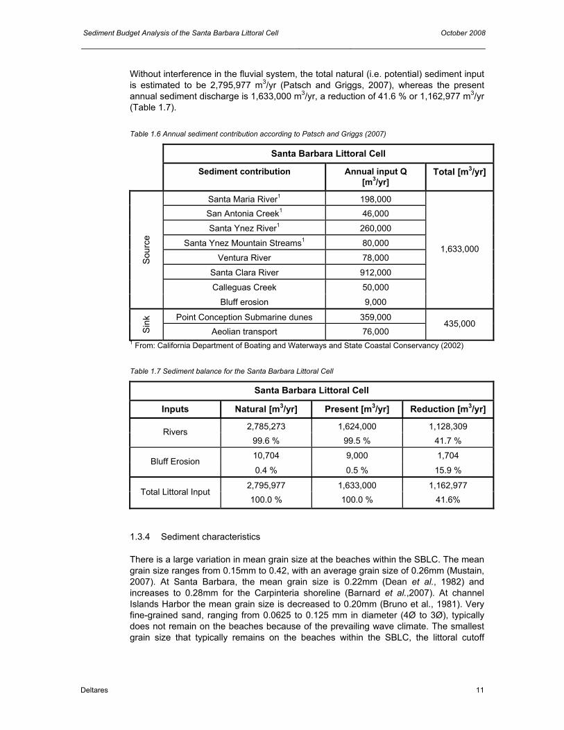
Without interference in the fluvial system, the total natural (i.e. potential) sediment input is estimated to be 2,795,977 m3/yr (Patsch and Griggs, 2007), whereas the present annual sediment discharge is 1,633,000 m3/yr, a reduction of 41.6 % or 1,162,977 m3/yr (Table 1.7). Table 1.6 Annual sediment contribution according to Patsch and Griggs (2007)
Santa Barbara Littoral Cell
Sediment contribution Annual input Q [m3/yr]
Total [m3/yr]
Santa Maria River1 198,000 San Antonia Creek1 46,000
Santa Ynez River1 260,000
Santa Ynez Mountain Streams1 80,000
Ventura River 78,000
Santa Clara River 912,000
Calleguas Creek 50,000
Sou
rce
Bluff erosion 9,000
1,633,000
Point Conception Submarine dunes 359,000
Sin
k
Aeolian transport 76,000 435,000
1 From: California Department of Boating and Waterways and State Coastal Conservancy (2002) Table 1.7 Sediment balance for the Santa Barbara Littoral Cell
Santa Barbara Littoral Cell
Inputs Natural [m3/yr] Present [m3/yr] Reduction [m3/yr]
2,785,273 1,624,000 1,128,309 Rivers 99.6 % 99.5 % 41.7 %
10,704 9,000 1,704 Bluff Erosion
0.4 % 0.5 % 15.9 %
2,795,977 1,633,000 1,162,977 Total Littoral Input
100.0 % 100.0 % 41.6%
1.3.4 Sediment characteristics
There is a large variation in mean grain size at the beaches within the SBLC. The mean grain size ranges from 0.15mm to 0.42, with an average grain size of 0.26mm (Mustain, 2007). At Santa Barbara, the mean grain size is 0.22mm (Dean et al., 1982) and increases to 0.28mm for the Carpinteria shoreline (Barnard et al.,2007). At channel Islands Harbor the mean grain size is decreased to 0.20mm (Bruno et al., 1981). Very fine-grained sand, ranging from 0.0625 to 0.125 mm in diameter (4Ø to 3Ø), typically does not remain on the beaches because of the prevailing wave climate. The smallest grain size that typically remains on the beaches within the SBLC, the littoral cutoff

October 2008 Sediment Budget Analysis of the Santa Barbara Littoral Cell
12 Deltares
diameter (LCD), is 0.125mm (Runyan and Griggs, 2003; Mustain, 2007; Barnard et al., 2007). The sediment from the Ventura River and the Santa Clara River is characterised by stratified layers of coarse sand (grain size between 0.5 – 1.0 mm on the Wentworth scale, see Appendix D) with relatively small amounts of gravel, clay and silt. At the downstream end of the Santa Clara River, the river bed is, on average, composed of 16% gravel, 64% (coarse) sand and 20% silt and clay, with a mean grain size (D50) of 0.76 mm (ENTRIX, 2002, as cited in Stillwater Sciences, 2007). 1.3.5 Littoral drift rates
Sediment inputs to littoral cells from coastal streams and cliff erosion are difficult to quantify. In addition, the distribution of sediment within a cell is difficult to determine due to the seasonal variation in dominant wave approach and the sensitivity of waves to the nearshore bathymetry. A rough estimate of the littoral drift can be obtained by long-term annual dredging rates of harbor entrance channels. In the SBLC, there are four harbors for which long-term dredging rates are available (Appendix C, Table C.1.2). In table 1.8, the average annual dredging volumes at these harbors are given. According to patsch and Griggs (2007), the Santa Barbara and Ventura Harbor are most suitable for determining long-term annual littoral drift rates within the SBLC. Because of the configuration of these harbors, together with the almost unidirectional net littoral drift from west to east, reversal transport from the downdrift beaches to the entrance channel occurs less frequent and the dredging volumes are believed to represent both the net and gross longshore transport rates (Patsch and Griggs, 2007). The average dredging rates for the Santa Barbara Harbor and the Ventura Habor are 240,000 m3/yr and 456,000 m3/yr, respectively. The dredged material is bypassed to the downcoast beaches to prevent erosion. Table 1.8 Mean annual dredging volumes in the Santa Barbara Littoral Cell (Patsch and Griggs, 2007)
Santa Barbara Littoral Cell
Sediment input Annual dredging volumes [m3/yr]
Santa Barbara Harbor 240,000
Ventura Harbor 456,000
Channel Islands Harbor 772,000
Port Hueneme 20,000
Sediment Budget Analysis of the Santa Barbara Littoral Cell October 2008
Deltares 13
2 Problem definition and objectives
2.1 Problem analysis
The majority of beaches within the Santa Barbara and Ventura County study area, with the exception of those in the Oxnard Plain, are narrow and ephemeral. The malnourished beaches continue to erode resulting in a reduction of the dry beach width, increase in damages by strom activity and decreased recreational beach benefits. Especially the beaches near the cities of Goleta (west end of Ellwood Beach, west end of Isla Vista Beach and Goleta Beach) and Carpinteria (Carpinteria States Beach) and the Ventura River mouth are facing coastal retreat due to short- and long-term erosion. The beaches in the Goleta region exhibit wide variability in width. Isla Vista exhibited a long-term erosion (narrowing) trend over the last 70 years: the beach volume has been decreased with 50% from 80,000 m2 to 40,000 m2 (Revell and Griggs, 2005). At Carpinteria state beach, the erosion rate is in the order of 0.5 m/yr (Hapke C.J. et al., 2006). Also the beach immediately downcoast of the Ventura River mouth is subject to significant erosion. The construction of a groin field has resulted in an accretion rate of 2.0 m/yr at Ventura Beach, whereas the beach that was present at the northern side of the groins however eroded rapidly with an erosion rate that exceeded -2.0 m/yr (Hapke C.J. et al., 2006). At present, most erosion problems within the region are thought to be related to human interferencees into the coastal system: damming and canalization of rivers, armouring of the coastline and disruption of the longshore sediment transport by the construction of breakwaters and jetties has reduced the sediment supply necessary to preserve the beaches. Nevertheless, stating that all erosion problems within the region are induced by the reduction of sediment input would be too straightforward. There might be parts of the coast that face coastal retreat due to the local wave climate rather than the lack of sediment supply. For long term coastal zone management purposes it is important to reveal the cause of the erosion, while wave induced erosion might need a totally different solution than erosion caused by a lack of sediment input. Up to now, the complicated morphodynamics are not yet completely understood. The United States Geological Survey (USGS) and the University of California, Santa Cruz (UCSC), are collaborating on a project to identify and quantify the pathways for near shore sediment transport for the coast within the Santa Barbara and Ventura Counties, California (Barnard, 2006). This project is supported by BEACON (Beach Erosion Authority for Clean Oceans and Nourishment), the City if Carpinteria and the USGS, and is conducted in collaboration with the United States Army Corps of Engineers (USACE). The aim of this study is to come up with a tool with which the understandings of the morphodynamics within the Santa Barbara Littoral Cell can be improved to predict the future coastal development and to assess potential performance of nourishment projects.
2.2 Research objectives
The main objective of this study is to identify and quantify the pathways of sediment transport within the Santa Barbara Littoral Cell, with emphasis on the sites where the shoreline erosion is critical. The key questions to be addressed questions are: (1) how does the morphological system in the Santa Barbara Littoral Cell actually work and (2)

October 2008 Sediment Budget Analysis of the Santa Barbara Littoral Cell
14 Deltares
what will the future coastline development be in the surroundings of the cities of Goleta, Carpinteria and Ventura? A numerical model is used to simulate the hydrodynamic and morphodynamic processes and to calculate the littoral drift rates. Subsequently, a regional sediment budget is proposed to provide insight into the net surplus or deficit of sediment over the modelling period. To answer these research questions, the main objective is divided into two sub-objectives:
• Determine the hydrodynamic and morphologic interaction within the Santa Barbara Littoral Cell
- What are the characteristics of the hydrodynamic forcing? - What are the characteristics of a reduced set of wave conditions that
can replace the full set of wave conditions and still represent the correct longshore sediment transport?
• Determine the long term morphologic behaviour within the Santa Barbara Littoral Cell.
- What are the characteristics of the longshore sediment transport? - What is the effect of the longshore sediment transport on the beaches
and what are the short- and long-term erosion and accretion trends? - Are the littoral drift rates limited by sediment supply or by wave forcing?
2.3 Research approach and Outline
A Delft3D Online Morphology model is used to meet the primary objective of this study. Chapter 3 elaborates on the construction of the model and the way in which the simulation is set up. Another objective of this study is to reduce the computational runtimes of the simulations by simplifying the hydrodynamic input conditions. The concept, as well as the implication of input reduction on the littoral drift rates within the Santa Barbara Channel, is described in chapter 4. To increase the models’ overall performance and to determine its sensitivity to some model parameters, a sensitivity analysis is performed that, together with a validation of the model, is described in chapter 5. Next chapter 6 elaborates on the pattern of the residual current and the littoral drift rates along the Santa Barbara Littoral Cell. Chapter 7 finally gives the conclusions drawn and recommendations for future work.

Sediment Budget Analysis of the Santa Barbara Littoral Cell October 2008
Deltares 15
3 Model description
3.1 Delft3D-Online (2DH) modelling approach
The Delft3D package is a process-based numerical model system that consists of a number of integrated modules. Together, these modules allow for the computation of hydrodynamic flow, water quality, ecological processes, short wave generation and propagation, sediment transport and morphological changes. The Delft3D-FLOW module is the heart of the framework of modules (Fig. 3.1) and aims to simulate non-steady tidal and/or meteorological-driven flows. By calling the other modules, additional processes (e.g. wave energy propagation and sediment transport) can be simultaneously (online) performed. Model simulations can be done in a one-dimensional (1D) mode in which averaging takes place in both vertical and horizontal direction, a two-dimensional horizontal or vertical (2DH and 2DV, respectively) mode or in a three-dimensional (3D) mode. The accuracy, as well as the computational effort, increases significantly with each dimension added.
Figure 3-1 The Delft3D software package. The heart of the framework is the FLOW-module.

October 2008 Sediment Budget Analysis of the Santa Barbara Littoral Cell
16 Deltares
Delft3D-FLOW module The main components in the Delft3D-Online modelling approach are the Delft3D-FLOW module and the Delft3D-WAVE module (Figure 3-2). The Delft3D-FLOW module (version 3.39.28) is the central module in the Delft3D-Online approach. It solves the non-linear shallow water equations that are derived from the three dimensional Navier Stokes equations for incompressible free surface flow, in two (depth-averaged) or three dimensions. The system of equations consists of the horizontal momentum equations, the continuity equation and the transport equations. While the water depth is assumed to be much smaller than the horizontal length scale, the shallow water assumption is valid. Under this assumption, the vertical momentum equation can be reduced to the hydrostatic pressure equation. The vertical accelerations are assumed to be small compared to the gravitational acceleration and are therefore not taken into account. A concise description of the basic flow equations is given in Appendix A. For a more detailed description reference is made to the Delft3D-FLOW User Manual (WL | Delft Hydraulics, 2006). Delft3D-WAVE module The effects of waves on flow (via forcing due to breaking, enhanced turbulence and bed shear stress) and the effects of flow on waves (via set-up, current refraction and enhanced bottom friction) are taken into account by online coupling of the Delft3D-FLOW and Delft3D-WAVE module. The wave effects are integrated in the flow simulation by executing the third-generation SWAN (Holthuijsen et al., 1993; Booij et al., 1999) wave processor (version 40.51A). The SWAN model solves the action balance equation in two dimensions of spectral and geographical space and in time, with which the evolution of random, short-crested waves are calculated. It accounts for wave refraction, propagation, wave-wave interaction, wave generation by wind, dissipation due to whitecapping, bottom friction and depth-induced wave breaking. The results of the wave simulation (significant wave height, peak spectral period, wave direction, mass fluxes, etc.) are included in the flow calculations through additional driving terms. In simulations where during the FLOW simulation the water level, bathymetry or flow velocity field changes significantly, it is desirable to call the WAVE module more than once (van Rijn and Walstra, 2003). The wave field can thereby be updated accounting for the changing water depths and flow velocities. The SWAN model can be performed in either the stationary or the non-stationary mode. Under the stationary assumption, the time component in the action balance equation is not taken into account, implying instantaneous wave propagation throughout the domain. No time steps are involved to compute the wave propagation, although some iterating is needed. By online coupling of the Delft3D-WAVE and FLOW module a so-called quasi-stationary calculation is performed, since the flow computations progress in time (i.e. non-stationary). In appendix A, a brief description of the basic formulae used in SWAN is given. For a more detailed description reference is made to the Delft3D-WAVE User Manual (WL | Delft Hydraulics, 2006). Sediment transport To account for the transport of non-cohesive sediment during flow simulations, the (default) transport formulations of Van Rijn (2000) are applied. In all these formulations, Van Rijn makes a distinction between bed load and suspended load, which both have a wave-related and a current-related contribution. Suspended load transport is calculated by solving the advection-diffusion equation for suspended sediment. Bed load transport refers to near-bed sediment transport occurring below van Rijn’s reference height,

Sediment Budget Analysis of the Santa Barbara Littoral Cell October 2008
Deltares 17
which is based on the bed roughness. Bed load transport responds almost instantaneously to changing flow conditions and orbital velocities within the wave-cycle. An overview of the transport formulations of Van Rijn (2000) is presented by Lesser et al. (2004) and summarized in Appendix A.
Figure 3-2 Modelling scheme of the Delft3D-Online Modelling approach. The Delft3D-FLOW module and
the Delft3D-Wave module are coupled to account for both the effects of waves on currents and the effect of flow on waves.
3.2 Computational grids
Two different horizontal computational grids are distinguished: a low resolution orthogonal grid and a high resolution curvi-linear grid. The first is used within the Delft3D-WAVE module while the latter is used in both the Delft3D-WAVE and the Delft3D-FLOW module (Figure 3.4). The low resolution wave grid has a spatial scale of 90 x 180 km to cover all physical obstacles within the area that might influence the propagation of wave energy into the Santa Barbara Channel (Figure 3-3). While Point Conception and the Northern Channel Island will refract, defract and dissipate the incoming wave energy, these obstacles are incorporated within low resolution wave grid. The cross-shore resolution (i.e. N-direction) varies from approximately 550 m (nearshore) to 1100 m (seaward model boundary). In the region of the Northern Channel Islands, the cross-shore resolution is refined to approximately 550 m to enable correct wave energy propagation between the islands. The longshore resolution (i.e. M-direction) is about 1100 m throughout the entire grid domain. In total, the low resolution wave grid has 22800 grid points (151 grid lines in both M and N direction). The high resolution curvi-linear flow grid is smaller than the large wave grid and covers the morphologic active zone. The western boundary is located 10 km east of Point Conception while the eastern boundary is located near Channel Islands Beach, Oxnard. The seaward boundary stretches about 12 km offshore to ensure that the entire morphologic active zone is captured by the flow grid. The longshore grid resolution increases from 1100 m at the western boundary to 500 m at the eastern side of the grid domain. At the seaward boundary, the cross-shore resolution is approximately 550 m (i.e. ~ the resolution of the coarse wave grid), whereas in the nearshore area it is increased to 20 m. In M-direction (i.e. longshore direction) the grid consists out of 260 grid lines and 119 grid lines in N-direction (i.e. cross-shore direction). In total, the high resolution flow grid consists out of 28600 grid cells.

October 2008 Sediment Budget Analysis of the Santa Barbara Littoral Cell
18 Deltares
Figure 3-3 Computational grids: wave grid (upper panel) and flow grid (lower panel). The flow grid is also
used as a nested wave grid to ensure a high grid resolution in the surf zone.

Sediment Budget Analysis of the Santa Barbara Littoral Cell October 2008
Deltares 19
3.3 Bathymetric schematisation
The model bathymetry is based on interpolation of depth samples that originate from multiple sources, each of different resolution. For the regions that experience significant erosion, near the cities of Goleta, Carpinteria and Ventura, the depth sample resolution is highest. For the 12 km stretch of coastline of the southwest facing Carpinteria Beach, bathymetric data was collected by the Coastal Profiling System (CPS), a hydrographic surveying system mounted on a Personal Watercraft (Barnard, 2007). The survey setup for this section contains of 36 cross-shore profiles running from approximately 1 km offshore through the surf zone and six alongshore profile parallel to the coastline. This bathymetric survey technique has been shown to achieve sub-decimetre accuracy (MacMahan, 2001, as cited in Barnard, 2007). The remaining part of the coastline in front of Carpinteria, up to almost 8 kilometres offshore, has a sample resolution of 20 m with a sub-decimetre accuracy (from USGS Submetrics, August 2005). In the Goleta Region, a similar CPS survey has been carried out immediately offshore of Isla Vista and West Beach, consisting of 41 cross-shore and 3 longshore profiles. In between the Ventura and Santa Clara River mouth, the CPS contains of 35 cross-shore profiles and 5 and 7 longshore profiles in front of the Ventura and Santa Clara River mouth, respectively. The remaining part of the nearhore bathymetry is based on 100 m resolution samples obtained from the SCOOS website (http://www.sccoos.ucsd.edu/data/bathy/?r=2). The bathymetry that covers the low resolution wave grid is based on depth soundings (200 m resolution) from NOAA (National Oceanic and Atmospheric Administration). The offshore and nearshore model bathymetry are illustrated in Appendix F, Fig. F.3.1 and F.3.2, respectively.
3.4 Parameter settings
The processes in the FLOW and WAVE modules are described by input parameters. Some of these parameters are widely used in process based models, while others are specific for this study. A complete overview of all model settings used in this study is given in Appendix C, Table C.3.1. 3.4.1 Parameter settings Delf3D-FLOW
Hydrodynamic time step The time step (∆t) for the flow computations is 30 seconds, based on the Courant number for wave propagation:
2 2
1 12 1waveCFL t gHx y
⎛ ⎞= ∆ + <⎜ ⎟∆ ∆⎝ ⎠
(3.1)
where ∆t is the time step, g is the acceleration of gravity, H is the total water depth and ∆x and ∆y are the smallest grid spaces. In models that have large differences in the geometry of the coastline, the Courant number should not exceed 10 (WL| Delft Hydraulics, 2006). In the nearshore area of the curvi-linear flow grid, the cross-shore resolution (∆x) is ~20 m and the long-shore resolution (∆y) is ~500 m. Flow simulations with different time steps (i.e. 6, 12, 30 and 60 seconds) have shown that for time steps up to ∆t =30sec the velocity fields are identical.

October 2008 Sediment Budget Analysis of the Santa Barbara Littoral Cell
20 Deltares
Boundaries Three open boundaries are applied at the flow grid: two lateral boundaries at the eastern and western side and one at the seaward side of the flow grid (Figure 3-4). The lateral boundaries are specified as Neumann boundaries (Roelvink and Walstra, 2004). Neumann boundaries specify an alongshore water level gradient imposed instead of a fixed water level. The seaward boundary (Figure 3-4, section A-B) is forced with a time varying tidal water level.
Figure 3-4 Open boundary conditions. At the seaward boundary (A-B), the water level is prescribed. At the
lateral boundaries (A-A’ and B-B’) the water level gradient as a function of time is imposed (so-called Neumann boundaries).
3.4.2 Parameter settings Delft3D-WAVE
Directional space The energy spectrum in SWAN is discretised with a constant directional resolution (∆θ). The directional space can be limited to reduce the computation time. The complicated geometry of the coastline and the presence of numerous breakwaters and jetties does not allow for a reduction of the directional space. The directional space covers the full circle (360°) and is divided into 72 directions with a constant directional resolution (∆θ) of 5°. Frequency space In the frequency domain, the lowest frequency must be slightly smaller than 0.6 times the lowest peak frequency expected, whereas the highest frequency must be at least 2.5 times the highest peak frequency expected (WL | Delft Hydraulics, 2006). While the wave climate in the SBLC solely consists of relatively low frequency swell (ƒ≈ 0.05 – 0.09 Hz), the lowest frequency is set to 0.02 Hz and the highest frequency is set to 0.5 Hz. The frequency resolution between these boundaries is not constant since the frequencies are logarithmically distributed. In total, 24 frequency bins are used to describe the frequency space. Boundary conditions The deep ocean wave climate is specified on the west, south and east side of the low resolution wave grid. While the deep ocean wave spectrum is assumed to be spatially homogeneous along the boundaries, uniform boundaries are used. For the shape of the frequency and the directional space, the default JONSWAP wave density spectrum is used with a peak enhancement factor 3.3 (default).

Sediment Budget Analysis of the Santa Barbara Littoral Cell October 2008
Deltares 21
Breaker parameter The breaker parameter (γ) is a dimensionless parameter in which the relation between the maximum wave height (Hmax) and the water depth (d) is incorporated. For a random wave field, Holthuijsen (2007) assumes that the breaker parameter is about 0.75. Empirical relations found by Battjes and Stive (1985) assume breaker parameters varying between 0.6 and 0.83, with an average of 0.73 for bathymetries with strong variations in bed level. Because the bathymetry within the Santa Barbara Channel varies from steep at the western side en relatively shallow at the eastern side of the model domain, the default value of 0.73 is used in this study. Bottom friction Dissipation of wave energy as a result of bottom friction is also accounted for in the SWAN module. The source term can be generally represented as:
( ) ( )2
,( , ) ,sinh
bfrbfr rms bottom
CS E u
g kdσσ θ σ θ
⎡ ⎤= − ⎢ ⎥
⎣ ⎦ (3.3)
in which bfrC is a bottom friction coefficient and ,rms bottomu is the root mean square orbital
bottom velocity (Holthuijsen, 2007). In this study, the empirical JONSWAP formulation of Hasselman et al. (1973) is used to describe the bottom friction coefficient:
,
0.038bfr JONSWAP
rms bottom
C Cu
= = (swell conditions) (3.4)
,
0.067bfr JONSWAP
rms bottom
C Cu
= = (wind-sea conditions) (3.5)
While the Santa Barbara Numerical Model is forced with relatively low frequency swell (ƒ≈ 0.05 – 0.09 Hz), the bottom friction coefficient ( bfrC ) as expressed in Eq. (3.4) is
used. Output parameters The computations within the SWAN module are performed in the stationary mode. While the water level and flow velocity field change significantly during the FLOW simulation, the WAVE module is called more than once (van Rijn and Walstra, 2003). The coupling interval is 150 minutes, so 11 alternating calls are made between the FLOW and WAVE module during each tidal cycle of 1500 minutes.

Sediment Budget Analysis of the Santa Barbara Littoral Cell October 2008
Deltares 23
4 Schematisation of boundary conditions
4.1 The concept of input reduction
One of the major problems in long-term morphological simulations is the difference in timescale between hydrodynamic and morphological processes. Most relevant morphological developments take place on a time-scale in the order of several or even tens of years, while hydrodynamic processes like waves and tides take place on a short time-scale ranging from seconds (waves) to hours (tides). To simulate both the hydro- and morphodynamics properly, a considerable amount of simulation time steps is required. The computer run-time will become large as well due to the linear relationship with the amount of time steps. In addition, the ever-increasing spatial scale of numerical models (i.e. the amount of grid cells involved) heavily appeals to the computer run-time. Generally, two approaches can be adopted to limit the computational effort (Steijn, 1992): simplification of the hydrodynamic input conditions and simplification of the physical processes. The first one is referred to as input filtering whereas the latter is referred to as process filtering. In this study, input filtering techniques are used to simplify the relevant hydrodynamic input conditions (tide and wave climate).
4.2 Schematisation of the wave climate
4.2.1 Introduction A way of reducing the run time for the simulation is to force the model with just these waves that contribute most to the longshore sediment transport. To determine the reduced a set of waves conditions, rough wave data first has to be classified in a wave climate table. All primary wave properties, like significant wave height (Hs), peak period (Tp), direction and probability of occurrence (P), are categorised into wave height and direction classes. Next, a reliable and preferably fast series of sediment transport computations with all wave conditions has to be performed. According to Steijn (1992), the simulation time of these simulations should preferably be equal to or a multiple of the tidal cycle period. Together, all these computations represent the average annual sediment transport induced by the entire wave climate. This average annual sediment transport is referred to as the target sediment transport, and forms the basis of the schematisation procedure. The tool that takes care of the schematisation procedure is the Opti-routine, which is solely based on statistical assumptions (WL|Delft Hydraulics, 2007). The schematisation relies on the relative contribution of each wave condition to the target sediment transport. The schematisation is not based on the sediment transport within the entire area, but only on the sediment transport through a number of predefined transects. The routine starts with the target sediment transport. First, with all conditions still participating, the contribution of condition i to the target is computed. In an iterative process, the wave condition (i.e. a sediment transport calculation) that contributes least to the target will be eliminated by setting its weight to zero. To what extend the remaining wave conditions resemble the target is based on the relative root mean square error (rmsRel). This term is defined as the relative root mean square error between the remainder and the target, divided by the root mean square of the target itself:

October 2008 Sediment Budget Analysis of the Santa Barbara Littoral Cell
24 Deltares
( )
( )
2
,1
2
1
D
id j jj
id D
jj
wad targetrmsRel
target
=
=
−=∑
∑ (4.1)
In which: D total number of data points id iterations step
jtarget target sediment transport at data point j
,id jwad weighted average of the sediment transport at data point j , using the
weights of iteration step id After the relative root mean square error has been defined, an iterative process randomly changes the weight factors of the remaining set of wave conditions. For each randomly determined new set of weight conditions, the relative root mean square error (rmsRel) is again calculated to determine the resemblance with the target. After all iterations, it is determined with which set of weights the target is resembled best by finding for which iteration the rmsRel is lowest. Next, the new set of weight conditions is used in the next elimination round (id+1). This process continues until only one condition is left. In Appendix B, a conceptual description of the iterative processes within the Opti-routine is given in a diagram.
4.2.2 Validation of the SWAN-model Prior to applying a wave schematisation for the Santa Barbara Channel, the performance of the SWAN-simulation is validated with inner-channel wave data. The SWAN parameter settings as described in the previous chapter are used. The wave grid is forced with hourly wave and wind conditions during a 12 hour storm, as registered by buoy 46063, located at the western entrance of the Santa Barbara Channel (see Figure 1-7). The simulated storm period ranges from December 8th 2007 06:00 to 17:00 hour (Figure 4-1). The storm period is randomly chosen, but depended on the availability of inner-channel buoy data. The inner-channel buoys used for validation are station 46216 (Goleta Point, location 34°20'1' N 119°38'13'' W, water depth 183 m) and station 46217 (Anacapa Passage, location 34°10'2' N 119°26'5'' W, water depth 110 m ). Station 46216 is located in the area of the high resolution flow grid, whereas station 46217 is, like station 46063, located on the low resolution wave grid. Wave and wind data is taken from the NDBC web site (http://www.ndbc.noaa.gov ) and summarized in Table 4.1. The validation is based on the significant wave height (Hs), the peak period (Tp) and the wave direction (Dir).

Sediment Budget Analysis of the Santa Barbara Littoral Cell October 2008
Deltares 25
Table 4.1 Primary conditions for station 46063, 46216 and 46217 during a 12 hour storm period at Dec. 8th 2007
Hs Tp Dir Ws WDir Hs Tp Dir Hs Tp Dir[m] [s] [°] [m/s] [°] [m] [s] [°] [m] [s] [°]
2007 12 08 06 : 00 5.91 12.12 286 10.5 310 2.99 11.76 257 3.06 12.50 2752007 12 08 07 : 00 5.89 12.12 297 12.1 309 2.89 12.50 256 3.16 11.76 2702007 12 08 08 : 00 6.18 12.08 290 11.7 309 3.39 12.50 257 3.04 12.50 2662007 12 08 09 : 00 6.43 12.18 293 11.8 319 3.28 12.50 256 2.97 12.50 2662007 12 08 10 : 00 5.70 12.12 295 11.5 327 3.34 11.76 264 3.00 11.11 2732007 12 08 11 : 00 5.38 12.90 300 10.2 325 3.02 11.76 263 2.77 12.50 2702007 12 08 12 : 00 5.30 11.43 298 10.0 322 2.72 12.50 266 2.55 12.50 2732007 12 08 13 : 00 5.42 12.12 303 10.9 315 2.76 12.50 260 2.69 13.33 2722007 12 08 14 : 00 5.28 12.12 306 10.4 308 2.70 10.53 263 2.73 12.50 2772007 12 08 15 : 00 5.30 12.90 303 10.8 319 2.37 11.76 271 2.64 12.50 2752007 12 08 16 : 00 5.37 12.12 305 11.0 312 2.38 11.76 260 2.59 13.33 2762007 12 08 17 : 00 5.19 12.12 301 11.0 312 2.09 11.11 262 2.40 10.53 275
46063 46216 46217
Timeseries
Figure 4-1 Time series of the significant wave height during a 12 hour storm period (red) at December 8th
2007 as registered by station 46063
In Figure 4-2, the differences between the measured (red) and simulated (blue) values of the wave height, peak period and direction is illustrated. The red dotted lines represent an error of 5% with respect to the measurements. While 46063 is located close to the model boundary, differences between the simulated and measured are limited. The peak period and the wave direction are in good agreement with the measurements, although the significant wave height is overestimated with about 2%. At station 46216, the differences between the simulation and the measurements have become larger. The error between the simulated and measured wave height occasionally exceeds 5%. The simulated wave direction follows the same increasing trend as the measured wave direction, although small variations are smoothed in the simulation and the simulated direction is on average slightly overestimated. At station 46217 the deviations in significant wave height and wave direction are largest, possibly caused by the relatively low resolution of the wave grid and the large distance between station 46217 and the western model boundary at which the storm conditions are applied. The wave direction is overestimated in the order of 15 degrees.

October 2008 Sediment Budget Analysis of the Santa Barbara Littoral Cell
26 Deltares
Figure 4-2 Validation of the SWAN-model, based on the significant wave height, wave period and wave
direction. Station 46063 is located close to the western model boundary, station 46216 is located in the Santa Barbara Channel (near Goleta) and station 46217 is located near Anacapa Passage.
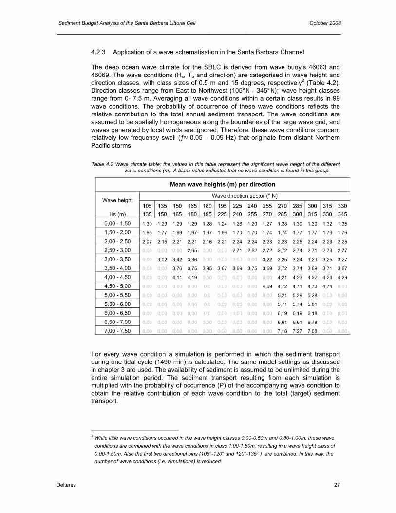
Sediment Budget Analysis of the Santa Barbara Littoral Cell October 2008
Deltares 27
4.2.3 Application of a wave schematisation in the Santa Barbara Channel The deep ocean wave climate for the SBLC is derived from wave buoy’s 46063 and 46069. The wave conditions (Hs, Tp and direction) are categorised in wave height and direction classes, with class sizes of 0.5 m and 15 degrees, respectively2 (Table 4.2). Direction classes range from East to Northwest (105°N - 345°N); wave height classes range from 0- 7.5 m. Averaging all wave conditions within a certain class results in 99 wave conditions. The probability of occurrence of these wave conditions reflects the relative contribution to the total annual sediment transport. The wave conditions are assumed to be spatially homogeneous along the boundaries of the large wave grid, and waves generated by local winds are ignored. Therefore, these wave conditions concern relatively low frequency swell (ƒ≈ 0.05 – 0.09 Hz) that originate from distant Northern Pacific storms. Table 4.2 Wave climate table: the values in this table represent the significant wave height of the different
wave conditions (m). A blank value indicates that no wave condition is found in this group.
Mean wave heights (m) per direction
Wave direction sector (° N) Wave height
105 135 150 165 180 195 225 240 255 270 285 300 315 330Hs (m) 135 150 165 180 195 225 240 255 270 285 300 315 330 345
0,00 - 1,50 1,30 1,29 1,29 1,29 1,28 1,24 1,26 1,20 1,27 1,28 1,30 1,30 1,32 1,35
1,50 - 2,00 1,65 1,77 1,69 1,67 1,67 1,69 1,70 1,70 1,74 1,74 1,77 1,77 1,79 1,76
2,00 - 2,50 2,07 2,15 2,21 2,21 2,16 2,21 2,24 2,24 2,23 2,23 2,25 2,24 2,23 2,25
2,50 - 3,00 0,00 0,00 0,00 2,65 0,00 0,00 2,71 2,62 2,72 2,72 2,74 2,71 2,73 2,77
3,00 - 3,50 0,00 3,02 3,42 3,36 0,00 0,00 0,00 0,00 3,22 3,25 3,24 3,23 3,25 3,27
3,50 - 4,00 0,00 0,00 3,76 3,75 3,95 3,67 3,69 3,75 3,69 3,72 3,74 3,69 3,71 3,67
4,00 - 4,50 0,00 0,00 4,11 4,19 0,00 0,00 0,00 0,00 0,00 4,21 4,23 4,22 4,24 4,29
4,50 - 5,00 0,00 0,00 0,00 0,00 0,0 0,00 0,00 0,00 4,69 4,72 4,71 4,73 4,74 0,00
5,00 - 5,50 0,00 0,00 0,00 0,00 0,0 0,00 0,00 0,00 0,00 5,21 5,29 5,28 0,00 0,00
5,50 - 6,00 0,00 0,00 0,00 0,00 0,0 0,00 0,00 0,00 0,00 5,71 5,74 5,81 0,00 0,00
6,00 - 6,50 0,00 0,00 0,00 0,00 0,0 0,00 0,00 0,00 0,00 6,19 6,19 6,18 0,00 0,00
6,50 - 7,00 0,00 0,00 0,00 0,00 0,00 0,00 0,00 0,00 0,00 6,61 6,61 6,78 0,00 0,00
7,00 - 7,50 0,00 0,00 0,00 0,00 0,00 0,00 0,00 0,00 0,00 7,18 7,27 7,08 0,00 0,00 For every wave condition a simulation is performed in which the sediment transport during one tidal cycle (1490 min) is calculated. The same model settings as discussed in chapter 3 are used. The availability of sediment is assumed to be unlimited during the entire simulation period. The sediment transport resulting from each simulation is multiplied with the probability of occurrence (P) of the accompanying wave condition to obtain the relative contribution of each wave condition to the total (target) sediment transport.
2 While little wave conditions occurred in the wave height classes 0.00-0,50m and 0.50-1.00m, these wave
conditions are combined with the wave conditions in class 1.00-1.50m, resulting in a wave height class of 0.00-1.50m. Also the first two directional bins (105°-120° and 120°-135° ) are combined. In this way, the number of wave conditions (i.e. simulations) is reduced.
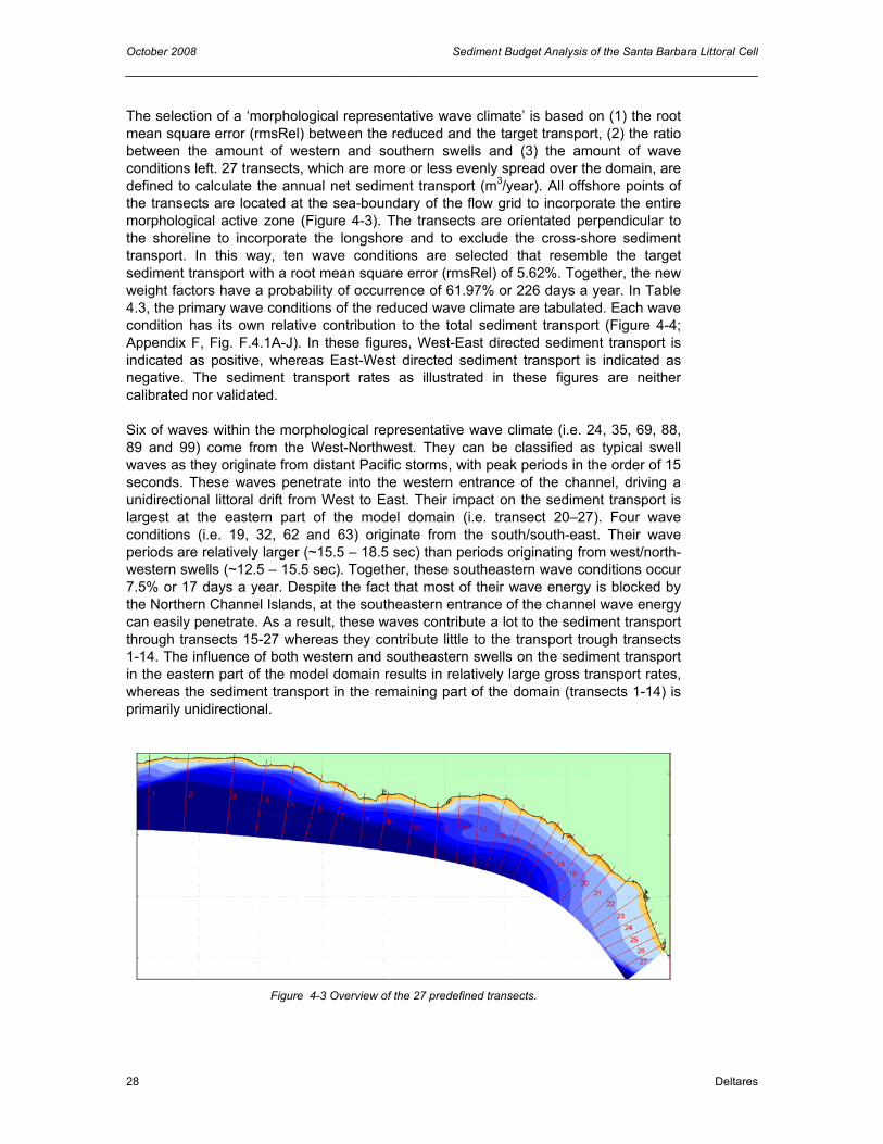
October 2008 Sediment Budget Analysis of the Santa Barbara Littoral Cell
28 Deltares
The selection of a ‘morphological representative wave climate’ is based on (1) the root mean square error (rmsRel) between the reduced and the target transport, (2) the ratio between the amount of western and southern swells and (3) the amount of wave conditions left. 27 transects, which are more or less evenly spread over the domain, are defined to calculate the annual net sediment transport (m3/year). All offshore points of the transects are located at the sea-boundary of the flow grid to incorporate the entire morphological active zone (Figure 4-3). The transects are orientated perpendicular to the shoreline to incorporate the longshore and to exclude the cross-shore sediment transport. In this way, ten wave conditions are selected that resemble the target sediment transport with a root mean square error (rmsRel) of 5.62%. Together, the new weight factors have a probability of occurrence of 61.97% or 226 days a year. In Table 4.3, the primary wave conditions of the reduced wave climate are tabulated. Each wave condition has its own relative contribution to the total sediment transport (Figure 4-4; Appendix F, Fig. F.4.1A-J). In these figures, West-East directed sediment transport is indicated as positive, whereas East-West directed sediment transport is indicated as negative. The sediment transport rates as illustrated in these figures are neither calibrated nor validated. Six of waves within the morphological representative wave climate (i.e. 24, 35, 69, 88, 89 and 99) come from the West-Northwest. They can be classified as typical swell waves as they originate from distant Pacific storms, with peak periods in the order of 15 seconds. These waves penetrate into the western entrance of the channel, driving a unidirectional littoral drift from West to East. Their impact on the sediment transport is largest at the eastern part of the model domain (i.e. transect 20–27). Four wave conditions (i.e. 19, 32, 62 and 63) originate from the south/south-east. Their wave periods are relatively larger (~15.5 – 18.5 sec) than periods originating from west/north-western swells (~12.5 – 15.5 sec). Together, these southeastern wave conditions occur 7.5% or 17 days a year. Despite the fact that most of their wave energy is blocked by the Northern Channel Islands, at the southeastern entrance of the channel wave energy can easily penetrate. As a result, these waves contribute a lot to the sediment transport through transects 15-27 whereas they contribute little to the transport trough transects 1-14. The influence of both western and southeastern swells on the sediment transport in the eastern part of the model domain results in relatively large gross transport rates, whereas the sediment transport in the remaining part of the domain (transects 1-14) is primarily unidirectional.
Figure 4-3 Overview of the 27 predefined transects.
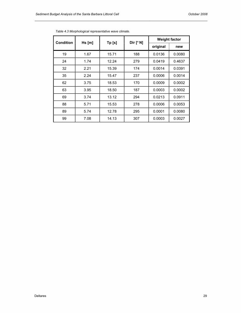
Sediment Budget Analysis of the Santa Barbara Littoral Cell October 2008
Deltares 29
Table 4.3 Morphological representative wave climate.
Weight factor Condition Hs [m] Tp [s] Dir [°N]
original new
19 1.67 15.71 188 0.0136 0.0080
24 1.74 12.24 279 0.0419 0.4637
32 2.21 15.39 174 0.0014 0.0391
35 2.24 15.47 237 0.0006 0.0014
62 3.75 18.53 170 0.0009 0.0002
63 3.95 18.50 187 0.0003 0.0002
69 3.74 13.12 294 0.0213 0.0911
88 5.71 15.53 278 0.0006 0.0053
89 5.74 12.78 295 0.0001 0.0080
99 7.08 14.13 307 0.0003 0.0027

October 2008 Sediment Budget Analysis of the Santa Barbara Littoral Cell
30 Deltares
Figure 4-4 Upper panel: comparison of the non-validated littoral drift rates for the entire (green) and the
reduced (yellow) wave climate. The relative root mean square error is 5.62%. Other panels: Individual sediment transport contribution for each wave condition within the schematised wave climate.

Sediment Budget Analysis of the Santa Barbara Littoral Cell October 2008
Deltares 31
4.2.4 Remarks The schematisation of the wave climate is based on the average yearly wave climate. Seasonal variations in wave climate, however, do exist. It is possible to schematise both the summer and winter wave climates separately, but this will result in an increase of the number of model computations. While rough wave conditions contribute relatively more to the total sediment transport than calm conditions, a schematisation of the wave climate based on the average yearly wave climate will lead to a slight underestimation of the total sediment transport (Steijn, 1989). Another remark is made with respect to the procedure with which the wave climate is schematised. The schematisation is based on the sediment transport through 27 predefined transects. As a result of this so called point-oriented procedure, the reduced set of wave conditions will represent only the sediment capacities at a few predefined points. This does not ensure a correct representation of the sediment transports in the whole area.
4.3 Schematisation of tidal currents
4.3.1 Introduction Tides are harmonic phenomena that have an important impact on both the hydrodynamics and the morphodynamics in a coastal area. For long-term morphological studies, it is therefore important to incorporate the effects of the tide in a proper way. Using real timeseries of the tide as an input for the model will lead to unnecessary high computational efforts (Latteux, 1995). To overcome this problem, the timeseries can be converted to a representative HW-LW tidal cycle. By harmonic analysis, the timeseries can be demodulated into a number of harmonic constituents that have their own unique amplitude, period and relative frequency. By reduction of the total set into a small set of tidal constituents, a simplified but representative HW-LW tidal cycle can be created with which the computational effort can be reduced significantly.
4.3.2 Application of a morphological tide in the Santa Barbara Channel The schematisation of the tide is based on a schematisation of the neap-spring tidal cycle. Usually, the neap-spring tidal cycle is represented by a mean tidal cycle. For morphological studies, however, this approach is not correct (Van Rijn, 1985, as cited in Steijn, 1989). The sediment transport (S) is proportional to the flow velocity (u) to a power (b):
bS u= (4.1) The maximum flow velocity during a tidal cycle is higher for larger tidal amplitudes. This implies that the contribution of the spring tide to the average sediment transport is relatively larger than the contribution of the neap tide. If a schematisation of the tide is based on a representation of the average sediment transport during a full neap-spring tidal cycle, a slight above-mean tide has to be chosen. This tide is referred to as the morphological tide (Steijn, 1989). It can be determined by increasing the velocities of the mean tidal cycle by multiplying its amplitude with a correction factor (τ). In general,

October 2008 Sediment Budget Analysis of the Santa Barbara Littoral Cell
32 Deltares
the value of the correction factor (τ) is approximately 1.1, with a standard deviation of about 0.1. The tidal data as presented in section 1.4.2 is indicated as the ‘astronomical tide’ and is compiled of a set of 11 constituents. Schematisation of the astronomical tide into a morphological tide with less constituents should not lead to significant differences in sediment transport. Furthermore, the flow patterns of both tidal representations should be similar. The morphological tide used in this study is compiled out of three constituents that have the largest contribution to the tidal water level variations (Table 4.4). Only one of these, the M2 constituent, accounts for the semi-diurnal distortion of the morphological tide, while the K1 and O1 constituents care for the diurnal character. For simplification, the angular frequencies of these constituents have been slightly adjusted to have a tidal period of the M2-constituent of 745 min and a tidal period of 1490 min for both the K1 and O1-constituent (Table 4.5). In this way, the K1 and O1-constituent have a period that is exactly twice the period of the M2-constituent, resulting in a morphological tide has a pure semi-diurnal character. The correction factor (τ) that has been applied has a value of 1.08. No sensitivity analysis has been carried out for this parameter while the relative contribution of the tide to the sediment transport is very low in comparison with the contribution of the waves. Table 4.4 Three tidal constituents that contribute most to the tidal water level variations.
Constituent Description Amplitude [m]
Angular frequency [deg/hr]
M2 Principal lunar semi-diurnal const. 0.4781 28.984104
K1 Lunisolar diurnal const. 0.3430 15.041052
O1 Lunar diurnal const. 0.2226 13.943052 Table 4.5 Morphological tidal constituents with their adjusted amplitude and angular frequency. The
angular frequency is adjusted to have a M2-period of exactly 745 min and periods of 1490 min for the K1 and O1 component. The amplitudes are multiplied by 1.08.
Constituent Description Amplitude [m]
Angular frequency [deg/hr]
M2 Principal lunar semi-diurnal const. 0.5163 28.993289
K1 Lunisolar diurnal const. 0.3704 14.496644
O1 Lunar diurnal const. 0.2404 14.496644 For both the morphological and the astronomical tide, a simulation is carried out with a simulation period of 14900 minutes (10 tidal cycles). In Figure 4-5, the simulation timeseries for both simulations are illustrated. The water level variation that results from multi-diurnal constituents, accounting for e.g. spring-neap cycles, is clearly observable for the time series of the astronomical tide. The morphological tide only has a diurnal and a semi-diurnal water level variation.

Sediment Budget Analysis of the Santa Barbara Littoral Cell October 2008
Deltares 33
Figure 4-5 Timeseries of the morphological tide (red) and the astronomical tide (blue).
The flow pattern for the morphological tide has a strong correlation with the flow pattern of the astronomical tide. During flood, the tidal current flows through the eastern entrance into the Santa Barbara Channel and flows out of the channel in the west. During ebb, the tidal current is directed opposite. The pattern of the residual current of the morphological tide is similar to the astronomical tide. Current magnitudes of the morphological tide are however underestimated with approximately 50 % (Figure 4-6). Consequently, the sediment transport is also significantly underestimated when using a morphological tide (Figure 4-7).
Figure 4-6 Residual current pattern for the astronomical tide (upper panel) and the morphological tide (lower
panel).

October 2008 Sediment Budget Analysis of the Santa Barbara Littoral Cell
34 Deltares
Figure 4-7 Residual sediment transport pattern for the astronomical tide (upper panel) and the
morphological tide (lower panel).
Although the tidal sediment transport is significantly being underestimated, the use of a morphological tide for this study is justified because of the low transport capacity of the tide relative to the waves. The tidal sediment transport capacity is in the order of 1.0 e-16 m3/sec, whereas the sediment transport capacity of the waves is in the order of 0.01 m3/sec. The minor effect of the tide to the sediment transport is illustrated in Figure 4-8. Two simulations are carried out during 10 tidal cycles, one with a morphological and one with an astronomical tide, in which the morphological representative wave climate as described in the previous section is included. The figure illustrates the net annual sediment transport through 27 transects (see Figure 4-3).
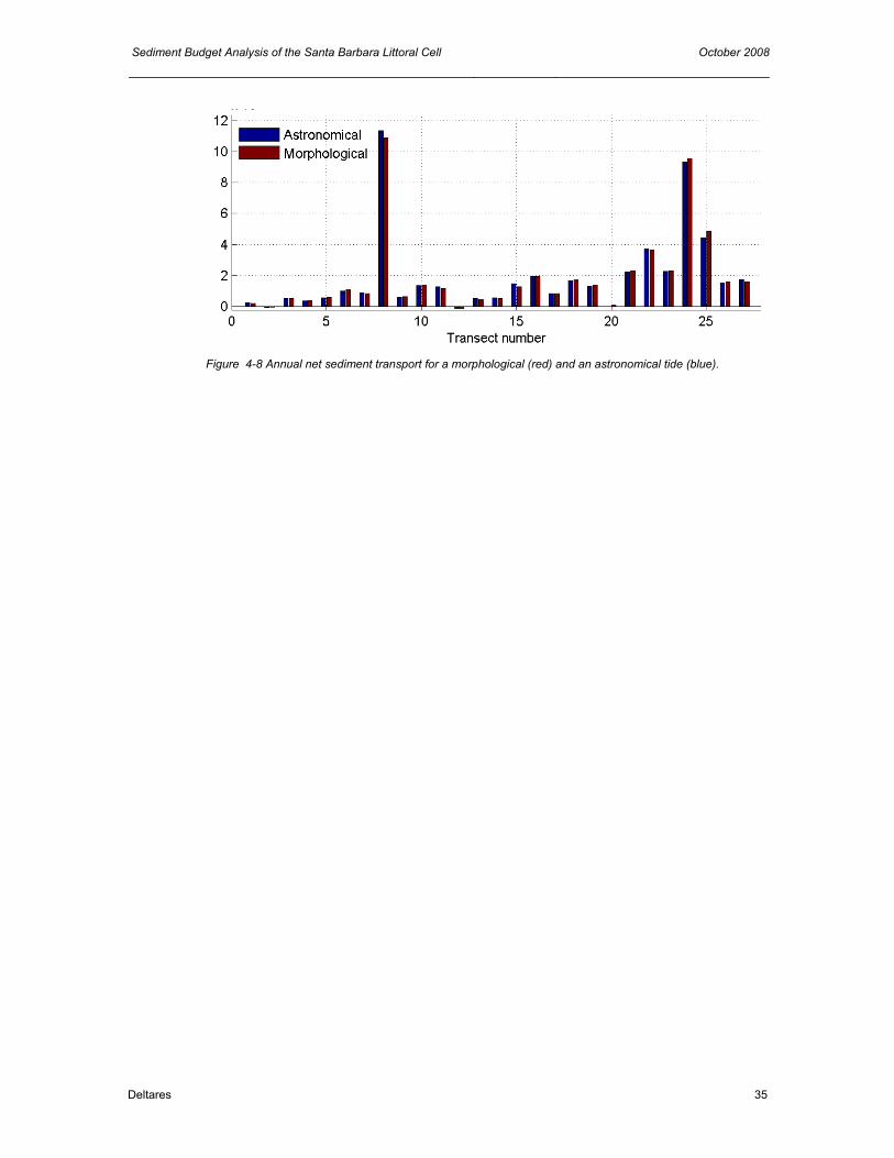
Sediment Budget Analysis of the Santa Barbara Littoral Cell October 2008
Deltares 35
Figure 4-8 Annual net sediment transport for a morphological (red) and an astronomical tide (blue).


Sediment Budget Analysis of the Santa Barbara Littoral Cell October 2008
Deltares 37
5 Sensitivity analysis
5.1 Introduction
A sensitivity analysis, based on the littoral drift through 28 transects, is performed to determine the models’ overall performance and its response to different model settings (Figure 5-1). The annual dredging rates of the entrance channels of the Santa Barbara Harbor and the Ventura Harbor (section 1.4.5) are used to validate the model. The dredging rates are compared with the sediment transport through transect 12 and 24, located just upcoast of the entrance channels. While the littoral drift is almost unidirectional (from West to East), the sediment transports through these transects are a good proxy for the dredging rates. All simulations are forced with the morphological tide and the morphological representative wave climate as discussed in the previous chapter.
Figure 5-1 Transects through which the littoral drift rates are determined. Transect 12 and 14 represent the
dredging volumes at the Santa Barbara and the Ventura Harbor, respectively.
The sensitivity of the model to parameter settings is determined for the grain size (D50), the current-related suspended and bed load parameter (sus/bed) and the wave-related suspended an bed load parameter (susw/bedw). The large variation in mean grain size along the beaches within the SBLC, necessitates a sensitivity analysis on the grain size (D50). It is an important parameter involved in the degree of sediment transport, while the particles resisting force on water motion is related to particle weight and friction coefficient. The current-related and the wave-related suspended and bed load parameters are calibration factors to adjust the overall significance of each transport component. For each parameter sensitivity analysis, only one parameter varies while all other parameters remain constant. The effect of the Ventura and Santa Clara River on the littoral drift rates is accounted for by including either the average annual river discharge or a peak river discharge. In these simulations, the models’ sensitivity to the river sediment fraction is investigated as well. In appendix E, the results of the sensitivity analysis summarized, including a simulation in which the combined effect of the newly derived parameters are combined.

October 2008 Sediment Budget Analysis of the Santa Barbara Littoral Cell
38 Deltares
5.2 Reference simulation
The relative effect of the model parameters on the littoral drift rates are compared with a reference simulation in which the parameter settings as discussed in chapter 3 are used (see also Appendix C, Table C.3.1). The current-related suspended and bed load parameters (sus/bed) have a default value of 1.0., whereas the wave-related components of the sediment transport (susw/bedw) have a value of 0.3. The grain size is 0.2 mm, slightly below the mean value of 0.26 mm. The river discharge of the Santa Clara and Ventura River is not taken into account into the reference simulation.
5.3 Scaling of the grain size
The grain size sensitivity analysis is based on sand with a single-fraction distribution within the entire model domain. The grain size diameters (D50) ranges from 0.125 - 0.42 mm. A diameter (D50) of 0.125 mm represents the Littoral Cut-off Diameter (LCD), whereas a D50 of 0.42 mm is the maximum grain size to be found on several beaches within the SBLC (Mustain, 2007). In Figure 5.2, simulations with grain sizes of 0.125, 0.20, 0.26, and 0.42 mm are compared. A grain size of D50=0.26 mm represents the mean grain size within the entire SBLC (Mustain, 2007). Large influence is noticed for the finest particle size of 0.125 mm. In particular the difference in transport between neighbouring transects (e.g. transects 23, 24 and 25) is larger for this diameter than for the larger diameters. The mean grain size of 0.26 mm shows a realistic pattern of the littoral drift rates, but slightly underestimates the transports at the Santa Barbara and Ventura Harbour (transects 12 and 24, respectively).
5.4 Scaling of the current-related suspended and bed load
The current-related suspended load transport is based on the variation of the suspended sediment concentration field due to the effects of currents and waves. The current-related bed load transport is based on a quasi-steady approach, which implies that the bed-load transport responds instantaneously to the current-velocity, and acts in the direction of the near-bed current (Van Rijn, 2004). The current-related calibration factors (sus/bed) have a lower and upper limit of 0.5 and 2.0, respectively. The default value of 1.0 implies a perfect representation of the physics of sand. The sensitivity of the current-related transport components is analysed by adjusting the sus and bed simultaneously in the range of 1.0 to 0.5 (Figure 5-3). A reduction of the sus/bed from 1.0 to 0.5 generally results in a reduction (up to 50%) of the littoral drift rates. Lowering the sus/bed loads to a larger deviation between the sediment transport through transect 12 and the Santa Barbara Harbor dredging results, whereas the sediment transport through transect 24 (Ventura Harbor) is hardly affected. The default value of 1.0 for the sus/bed parameters seems to be a good proxy for the dredging rates.

Sediment Budget Analysis of the Santa Barbara Littoral Cell October 2008
Deltares 39
Figure 5-2 Influence of the grain size (D50) on littoral drift rates
Figure 5-3 Influence of the current related suspended and bed load parameter (sus/bed) on littoral drift rates

October 2008 Sediment Budget Analysis of the Santa Barbara Littoral Cell
40 Deltares
5.5 Scaling of the wave-related suspended and bed load
The wave-related transport components for bed and suspended load (susw/bedw) acts in the direction of the wave propagation. In the surf zone, this implies that the wave-related transport component is responsible for the onshore-directed transports. While the sensitivity analysis is based on the littoral transport, variations in the wave-related transport factors (susw/bedw) should not have much effect. In regions where the waves, despite refraction, break at an angle with respect to the shoreline, the influence of the susw/bedw can however be significant. In the sensitivity analysis, calibration factors in the range of 0.0 (no wave related suspended and bed load) to 1.0 are applied. In Figure 5-4, the mean total transport resulting from wave condition 19 is presented to indicate the effect of the wave-related transport component. The black vectors indicate the sediment transport resulting from a susw/bedw value of 1.0, whereas the red vectors refer to a susw/bedw of 0.0. The effect of the susw/bedw on the onshore component is apparent.
Figure 5-4 Effect of susw/bedw on the littoral drift
In Figure 5-5, the influence of the susw/bedw on the littoral drift rates is shown. The largest effects are noticeable in the eastern region of the model domain (i.e. transects 24, 25, 26), where southern swell waves approach the coastline under large oblique angles. While the angle of wave approach is one of the main components that drive the littoral current, variation of the susw/bedw parameter has significant effects on the littoral drift rates. The variation in littoral drift will be enlarged for transects that are not completely perpendicular to the shoreline. Based on the dredging rates, a susw/bedw value of 1.0 exaggerates the littoral drift rates with 30% and 80%, whereas a value of 0.3 underestimates the littoral drift rates with 40% and 50% for the Santa Barbara and Ventura Harbor, respectively. With a susw/bedw value of 0.4, a reasonable proxy for the dredging rates is obtained.

Sediment Budget Analysis of the Santa Barbara Littoral Cell October 2008
Deltares 41
Figure 5-5 Influence of the wave related suspended and bed load parameter (susw/bedw) on littoral drift
rates
5.6 River discharge
5.6.1 Average annual river discharge
The average annual river discharge, based on a timeseries of 14 years (section 1.4.3), is 7.51 m3/sec and 2.77 m3/sec for the Santa Clara River and the Ventura River, respectively. Concentration rates (C) are derived from the relation between the annual sediment delivery (Table 1.6, section 1.4.3) and the annual water discharge, and are 10.20 kg/m3 for the Santa Clara River and 2.27 kg/m3 the Ventura River. The mean grain size (D50) at the downstream end of the Santa Clara River is 0.76 mm (Stillwater Sciences, 2007). In the sensitivity analysis, the above mentioned river discharges and concentrations are applied with fluvial grain size varying from 0.125 mm (littoral cut-off diameter) to 0.76 mm. The fluvial sediment concentration is primarily bounded between the mainland and the -30-depth contour (Figure 5-6). The littoral sediment transport is only affected upcoast of the Santa Clara River mouth (Figure 5-7). Variations in the grain size of the river sediment fraction do not have a significant effect on the littoral drift rates.
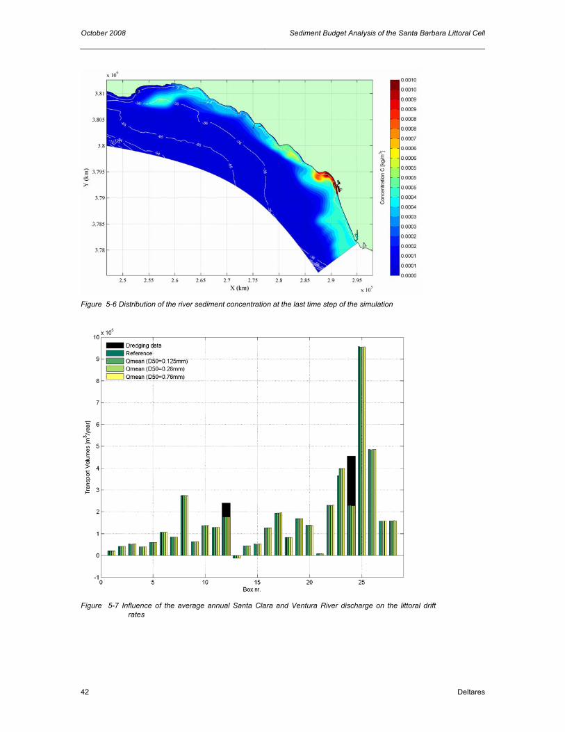
October 2008 Sediment Budget Analysis of the Santa Barbara Littoral Cell
42 Deltares
Figure 5-6 Distribution of the river sediment concentration at the last time step of the simulation
Figure 5-7 Influence of the average annual Santa Clara and Ventura River discharge on the littoral drift
rates

Sediment Budget Analysis of the Santa Barbara Littoral Cell October 2008
Deltares 43
5.6.2 Flood river discharge
As stated in section 1.4.3, hypopycnal flows account for nearshore delta formation, whereas hyperpycnal flows deposit sediment in the offshore delta. The mean annual flood discharge (Qmaf), which is statistically defined to be the 2.33 yr recurrence interval peak discharge, can be seen as an upper boundary at which hypopycnal flows takes place (Warrick et. al., 2003). In the sensitivity analysis of the flood river discharge, a hypopycnal flow is simulated, while the nearshore delta deposits are subject to wave impact and longshore transport. For the Santa Clara River, the mean annual flood discharge (Qmaf) , is 520 m3/s. No data on the mean annual flood discharge of the Ventura River is available. While the ratio of the average annual discharge between the Santa Clara River and the Ventura River is 2.7 (see section 5.6.1), the mean annual flood discharge Qmaf for the Ventura River is determined to be 192 m3/s. The sediment concentration is 40 g/l, which is the hypopycnal upper bound. The simulation period is 60 hours. While the mean annual flood discharge (Qmaf) is a hypopycnal flow, the distribution pattern of the fluvial sediment fraction is the same as for the simulation in which the average annual river discharge is used (see Figure 5-7). The littoral drift rates show a slight increase in the region of the Santa Clara River mouth (transect 23 -25). A variation in the diameter of the grain size does not have any significant impact on the littoral drift rates (Figure 5-8).
Figure 5-8 Influence of the mean annual Santa Clara and Ventura River flood discharge on the littoral drift
rates

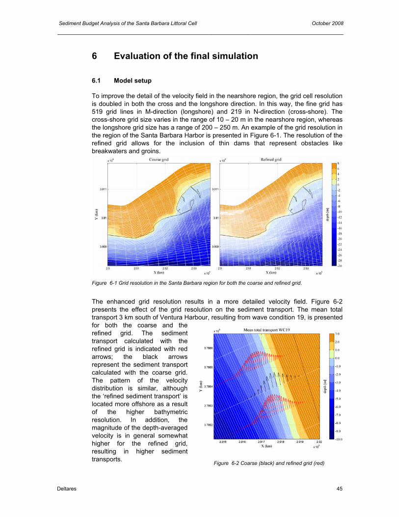
Sediment Budget Analysis of the Santa Barbara Littoral Cell October 2008
Deltares 45
6 Evaluation of the final simulation
6.1 Model setup
To improve the detail of the velocity field in the nearshore region, the grid cell resolution is doubled in both the cross and the longshore direction. In this way, the fine grid has 519 grid lines in M-direction (longshore) and 219 in N-direction (cross-shore). The cross-shore grid size varies in the range of 10 – 20 m in the nearshore region, whereas the longshore grid size has a range of 200 – 250 m. An example of the grid resolution in the region of the Santa Barbara Harbor is presented in Figure 6-1. The resolution of the refined grid allows for the inclusion of thin dams that represent obstacles like breakwaters and groins.
Figure 6-1 Grid resolution in the Santa Barbara region for both the coarse and refined grid.
The enhanced grid resolution results in a more detailed velocity field. Figure 6-2 presents the effect of the grid resolution on the sediment transport. The mean total transport 3 km south of Ventura Harbour, resulting from wave condition 19, is presented for both the coarse and the refined grid. The sediment transport calculated with the refined grid is indicated with red arrows; the black arrows represent the sediment transport calculated with the coarse grid. The pattern of the velocity distribution is similar, although the ‘refined sediment transport’ is located more offshore as a result of the higher bathymetric resolution. In addition, the magnitude of the depth-averaged velocity is in general somewhat higher for the refined grid, resulting in higher sediment transports.
Figure 6-2 Coarse (black) and refined grid (red)

October 2008 Sediment Budget Analysis of the Santa Barbara Littoral Cell
46 Deltares
The simulation time step (∆t) for the hydrodynamic calculations is decreased from 30 seconds to 15 seconds to ensure numerical stability. The mean grain size diameter (D50) of 0.26 mm (Wentworth scale: medium sand) is used to represent the sediment within the entire model domain. The wave and current-related sediment transport calibration factors are 0.4 and 1.0, respectively, based on the sensitivity analysis as describes in chapter 5. The river discharge is simulated as an average annual river discharge instead of a mean flood discharge, while the spreading of the fluvial sediment fraction within the area is more realistic for the first than for the latter. The annual Santa Clara River discharge (Qmean) is 7.51 m3/sec with a concentration rate (C) of 10.20 kg/m3; the annual discharge (Qmean) of the Ventura River is 2.77 m3/sec and has an average concentration rate (C) of 2.27 kg/m3. The grain size diameter (D50) of the fluvial sediment fraction is 0.76 mm (Wentworth scale: coarse sand).
6.2 Analysis of the residual current
6.2.1 Tidal current The residual current is compiled of a tidal and a wave driven (i.e. littoral current) component, and is obtained by Fourier analysis of the velocity field. Relative to the littoral current, the tidal current contribute less to the total sediment transport along the coast. Still, the tidal current can (locally) transport sediment, while acceleration of flow due to convergence of flow streamlines locally can increase the velocities up to 2 m/s. The California Current (CC) and its counterpart, the Southern California Countercurrent (SCC), dominate the flow pattern within the Santa Barbara Channel (Hickey, 1992). The SCC enters the Santa Barbara Channel between Anacapa Islands and the mainland, and flows along the mainland in western direction (Figure 6-3). Figure 6-4 and 6-5 illustrate the velocity field and the sediment transport patterns, respectively, during flood (a) and ebb (b). In case of flood (Figure 6-4a), the sediment transport enters the Santa Barbara Channel from the south-southeast, through the entrance between the Northern Channel Islands and the mainland. Shortly after the tidal sediment transport enters the model domain, the transport trajectory bends towards the coastline, along which it flows towards the west/northwest. From the City of Carpinteria, the tidal sediment transport is bounded within a narrow flume that is directed from East to West. For ebb-tidal flows, the current is directed opposite, with relatively low maximum velocities being in the order of 1.0 cm/s (Figure 6-4b).
Figure 6-3 Circulation pattern in the Southern California Bight http://seis.natsci.csulb.edu/bperry/scbweb/

Sediment Budget Analysis of the Santa Barbara Littoral Cell October 2008
Deltares 47
The residual tidal current during one tidal simulation period shows a similar pattern as for the ebb- and flood tidal flows (Figure 6-4c). In general, the residual tidal sediment transport along the coastline is directed opposite to the littoral current. At locations that are mostly sheltered from wave energy (e.g. just downcoast of the Cities of Goleta and Santa Barbara), little east-westwards directed sediment transport can be expected.
Figure 6-4 Tidal current pattern for (a) flood, (b) ebb and (c) residual.

October 2008 Sediment Budget Analysis of the Santa Barbara Littoral Cell
48 Deltares
Figure 6-5 Tidal sediment transport pattern for (a) flood, (b) ebb and (c) residual.

Sediment Budget Analysis of the Santa Barbara Littoral Cell October 2008
Deltares 49
6.2.2 Residual Current The residual current is determined by Fourier analysis of the velocity field, accounting for both the effect of tides and waves. By setting the number of cycles within the analysis time frame to zero, the mean velocity for each simulation (i.e. wave condition) is obtained. The residual current results from the weighted average of the mean velocities of all (10) wave conditions within the morphological representative wave climate. The model domain is divided into seven sections (Figure 6-6). Focus sites are near the cities of Goleta and Carpinteria and the Ventura and Santa Clara River Delta (sections 3, 5 and 7), where significant shoreline erosion endangers the subsistence of the beaches.
Figure 6-6 Subdivision of the model domain. Sections 3, 5 and 7 (indicated in red) represent the focus sites.
Figure 6-7 illustrates the energy dissipation for wave condition 62 (southern swell) and wave condition 88 (western swell) to indicate the effect of the wave direction on energy concentrations. Section 3 covers the Goleta Platform, a protrusion that encounters high wave energy concentrations in case of western swells. Especially at Ellwood Beach (upcoast of Coal Oil Point) and Isla Vista Beach (in between Coal Oil Point and Goleta Point) is subject to high energy loads from western swells. The eastern flank of the Goleta Platform is almost completely sheltered from wave energy for both western and southern swells. Along the entire coastline within section 5, near the city of Carpinteria, high energy dissipation rates arise for both western and southern swells. In particular the coastlines downdrift of the Carpinteria State Beach and orth of Sandy Point, are exposed to high wave energy loads. Section 7 covers the Ventura and Santa Clara River Delta. In case of southern swells, most energy dissipation occurs north of the Ventura River mouth and south of the Santa Clara River mouth. In between, near the Ventura Harbor, the coastline is located more inland, resulting in less exposure to wave energy from southern swells. For western swells, no sheltering effect due to the coastline orientation occurs, resulting in high energy dissipation rates in the region of the Ventura Harbor. The pattern of the residual current, which accounts for the combined effect of the tidal and littoral current, is dominated by the littoral current and is directed from West to East/SouthEast. For section 1 to 7, the residual current is illustrated to indicate the pattern of the velocity field (Figure 6-9 – Figure 6-13).
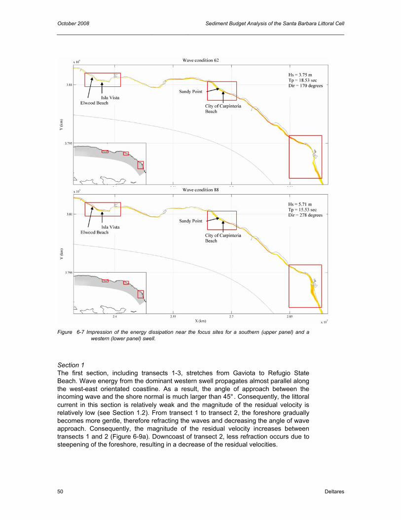
October 2008 Sediment Budget Analysis of the Santa Barbara Littoral Cell
50 Deltares
Figure 6-7 Impression of the energy dissipation near the focus sites for a southern (upper panel) and a
western (lower panel) swell.
Section 1 The first section, including transects 1-3, stretches from Gaviota to Refugio State Beach. Wave energy from the dominant western swell propagates almost parallel along the west-east orientated coastline. As a result, the angle of approach between the incoming wave and the shore normal is much larger than 45°. Consequently, the littoral current in this section is relatively weak and the magnitude of the residual velocity is relatively low (see Section 1.2). From transect 1 to transect 2, the foreshore gradually becomes more gentle, therefore refracting the waves and decreasing the angle of wave approach. Consequently, the magnitude of the residual velocity increases between transects 1 and 2 (Figure 6-9a). Downcoast of transect 2, less refraction occurs due to steepening of the foreshore, resulting in a decrease of the residual velocities.
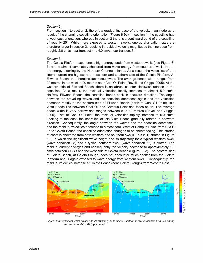
Sediment Budget Analysis of the Santa Barbara Littoral Cell October 2008
Deltares 51
Section 2 From section 1 to section 2, there is a gradual increase of the velocity magnitude as a result of the changing coastline orientation (Figure 6-9b). In section 1, the coastline has a west-east orientation, whereas in section 2 there is a southward bend of the coastline of roughly 25°. While more exposed to western swells, energy dissipation rates are therefore larger in section 2, resulting in residual velocity magnitudes that increase from roughly 2.0 cm/s near transect 4 to 4.0 cm/s near transect 6. Section 3 The Goleta Platform experiences high energy loads from western swells (see Figure 6-7) and is almost completely sheltered from wave energy from southern swells due to the energy blocking by the Northern Channel Islands. As a result, the velocities of the littoral current are highest at the western and southern side of the Goleta Platform. At Ellwood Beach, the shoreline faces southwest. The average beach width ranges from 20 metres in the west to 90 metres near Coal Oil Point (Revell and Griggs, 2005). At the western side of Ellwood Beach, there is an abrupt counter clockwise rotation of the coastline. As a result, the residual velocities locally increase to almost 5.0 cm/s. Halfway Ellwood Beach, the coastline bends back in seaward direction. The angle between the prevailing waves and the coastline decreases again and the velocities decrease rapidly at the eastern side of Ellwood Beach (north of Coal Oil Point). Isla Vista Beach lies between Coal Oil and Campus Point and faces south. The average beach width is very narrow and ranges between 5 to 40 metres (Revell and Griggs, 2005). East of Coal Oil Point, the residual velocities rapidly increase to 6.0 cm/s. Looking to the east, the shoreline of Isla Vista Beach gradually rotates in seaward direction. Consequently, the angle between the waves and the coastline decreases, and the residual velocities decrease to almost zero. West of Campus Point, from UCSB up to Goleta Beach, the coastline orientation changes to southeast facing. This stretch of coast is sheltered from both western and southern swells. This is illustrated in Figure 6-8, in which the significant wave height and its trajectory for a typical western swell (wave condition 88) and a typical southern swell (wave condition 62) is plotted. The residual current diverges and consequently the velocity decrease to approximately 1.0 cm/s between UCSB and the west side of Goleta Beach (Figure 6-9c). The eastern side of Goleta Beach, at Goleta Slough, does not encounter much shelter from the Goleta Platform and is again exposed to wave energy from western swell. Consequently, the residual velocities increase at Goleta Beach (near Goleta Slough) from West to East.
Figure 6-8 Significant wave height and its trajectory near Goleta Platform for wave condition 88 (left panel)
and wave condition 62 (right panel).

October 2008 Sediment Budget Analysis of the Santa Barbara Littoral Cell
52 Deltares
Figure 6-9 Residual current pattern for (a) section 1, (b) section 2, (c) section 3 and (d) section 4.

Sediment Budget Analysis of the Santa Barbara Littoral Cell October 2008
Deltares 53
Section 4 For this section, the same pattern as for the Goleta Platform is observed. At the western side, between transect 9 and 10, the direction of the coastline changes from West-East to Northwest-Southeast, the foreshore steepens and the surfzone becomes more narrow (Figure 6-9d). As a result, the residual current is converged and the velocities increase to 6.0 cm/s near transect 10. The residual velocity remains approximately constant from transect 10 to transect 12 (west of Leadbetter Beach). From there, the coastline faces southeast and is sheltered from wave energy from western swells. The foreshore becomes more flat and the surf zone widens, resulting in a divergence of the residual current and a decrease in the residual velocities. The decrease of the residual velocity continuous, until eventually at the Santa Barbara Habor the residual current is nearly diminished. West Beach (transect 13), is located immediately adjacent to the harbour breakwater and west of East Beach. It is completely sheltered from western swells due to the coastline orientation and the breakwater configuration (Figure 6-10, lower panel). Occasionally, West Beach experiences energy loads from south-eastern swells (Figure 6-10, upper panel), resulting in an east-west direction of the residual current. Between transect 13 and 14, the influence of the western swell energy is noticeable again: the residual current is directed from West to East and increases to 4 cm/s at transect 14.
Figure 6-10 Significant wave height and its trajectory near Santa Barbara Platform for wave condition 62
(upper panel) and wave condition 88 (lower panel).

October 2008 Sediment Budget Analysis of the Santa Barbara Littoral Cell
54 Deltares
Section 5 From section 4 to 5, there is a rather abrupt clockwise rotation (~40°) of the coastline. In this region, the coastline is no longer dominated by western swell. Wave energy from south/southeastern swell reaches the coastline on a regular basis, resulting in an upcoast directed littoral current. The effect it has on the residual current is illustrated in Figure 6-10. The red arrows indicate the trajectory of wave condition 62 (Hs= 3.75 m, Dir = 170°N). The black arrows indicate the trajectory of wave condition 88 (Hs=5.71 m, Dir = 278°N). At the riprap backed stretch of coastline just North of Sandy Point, near Sandyland, the angle of wave approach (φ) with respect to the shore normal is about equal but opposite for the southern and western swells (Figure 6-10). Consequently, the residual current velocities are relatively low in the region of Sandyland (Figure 6-11). East of Carpinteria State Beach, the coastline rotates counterclockwise, resulting in a decrease of the angle (φ) for southern swells and an increase of (φ) in case of western swells. As a result, the littoral current is dominated by the western swell and the residual velocities are directed to the south/southeast and increase up to 6 cm/s near transect 17 (Rincon Beach).
Figure 6-12 Residual current pattern for section 5.
Figure 6-11 Trajectory for (red) wave condition 62 (dir=170°N)
and (black) wave condition 88 ( dir =278°N).
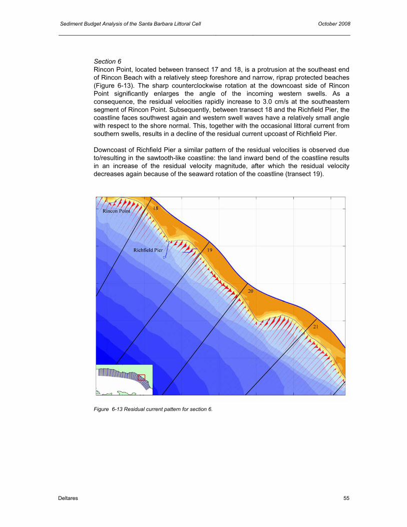
Sediment Budget Analysis of the Santa Barbara Littoral Cell October 2008
Deltares 55
Section 6 Rincon Point, located between transect 17 and 18, is a protrusion at the southeast end of Rincon Beach with a relatively steep foreshore and narrow, riprap protected beaches (Figure 6-13). The sharp counterclockwise rotation at the downcoast side of Rincon Point significantly enlarges the angle of the incoming western swells. As a consequence, the residual velocities rapidly increase to 3.0 cm/s at the southeastern segment of Rincon Point. Subsequently, between transect 18 and the Richfield Pier, the coastline faces southwest again and western swell waves have a relatively small angle with respect to the shore normal. This, together with the occasional littoral current from southern swells, results in a decline of the residual current upcoast of Richfield Pier. Downcoast of Richfield Pier a similar pattern of the residual velocities is observed due to/resulting in the sawtooth-like coastline: the land inward bend of the coastline results in an increase of the residual velocity magnitude, after which the residual velocity decreases again because of the seaward rotation of the coastline (transect 19).
Figure 6-13 Residual current pattern for section 6.

October 2008 Sediment Budget Analysis of the Santa Barbara Littoral Cell
56 Deltares
Section 7 At the Ventura River mouth (transect 23), the coastline orientation abruptly changes to south facing and the residual current increases significantly in west-east direction. The cause of this increase is illustrated in Figure 6-14. Near the Ventura River mouth, the little refracted western swell (e.g. wave condition 88, Hs=5.71 m, Dir = 278°N) has an angle of wave approach (φ) close to 45°. In this region, swell from the south (e.g. wave condition 62, Hs= 3.75 m, Dir = 170°N) will approach the coast almost perpendicular. The western swell dominates the littoral current along this stretch of coastline. The residual velocities are directed west-east and reach a maximum of 6.0 cm/s just south of transect 23 (Figure 6-15).
Figure 6-14 Significant wave height and its trajectory near Ventura Harbor for wave condition 88 (left panel)
and wave condition 62 (right panel).
Subsequently, the coastline rotates seaward to approximately 60° with respect to the west-east orientation. This, together with the presence of multiple groins and the Ventura Harbor configuration, decelerates the residual current. Just upcoast of the Ventura Harbor, the angle of wave approach (φ) with respect to the shore normal is for both southern en western swells relatively small and, consequently, the residual velocities are negligible (Figure 6-15). At the mouth of the Santa Clara River, between transect 24 and 25, the foreshore is gently sloping by fluvial sediment delivery. The effect of both western and southern swells on the residual velocities is apparent. The residual current is dominated by southern swell wave energy just downcoast of the Ventura Harbor, while the breakwater configuration of the harbor locally shelters the coastline from western swell wave energy. Subsequently, the western swell wave energy dominates the residual current again at the Santa Clara River mouth and at McGrath State Beach (between transect 25 and 26). Although the residual velocities south of the Santa Clara River mouth are dominated by the western swells and directed south, southern swells do have a significant effect. Consequently, the gross velocities are large along this part of the coastline.

Sediment Budget Analysis of the Santa Barbara Littoral Cell October 2008
Deltares 57
Figure 6-15 Residual current pattern for section 7.

October 2008 Sediment Budget Analysis of the Santa Barbara Littoral Cell
58 Deltares
Figure 6-16 Residual sediment transport vectors for the Santa Barbara Channel.

Sediment Budget Analysis of the Santa Barbara Littoral Cell October 2008
Deltares 59
6.3 Analysis of the littoral drift
Littoral drift is induced by the littoral current that is driven by the radiation stress of waves approaching under an angle. The complex geometry of the SBLC coastline causes spatial differences in the magnitude of the residual flow velocities. Changes in coastline orientation (either abrupt or gradual), alongshore water depth variations and variations in the width of the surf zone, (locally) results in a velocity gradient of the littoral current. For a sandy coast, the gradient in the littoral current will result in a longshore variation of the littoral drift, causing the coastline either to accrete or to erode. While in the simulation unlimited sediment supply is assumed and the entire coastline of the SBLC is modelled as a sandy coast, the pattern of littoral drift rates reflects the pattern of the residual current. A gradient in the residual current therefore results in a gradient of the littoral drift rates.
Figure 6-17 Littoral drift rates for the Santa Barbara Channel
Figure 6-16 and Figure 6-17 illustrate the spatial variation of the littoral drift along the coastline of the Santa Barbara Channel. The simulated littoral drift rates through the transects upcoast of the Santa Barbara and Ventura Harbor are in good agreement with the annual dredging rates. The error between the simulated littoral drift rates and the dredging rates is in the order of 10%, with the simulated transport rates being underestimated. Taking the minor reversal transport at transect 13 into account, this underestimation is partly counteracted. At locations where the coastline consists of sandy beaches, the gradient in the littoral drift curve gives an indication on the erosion/accretion trends to be expected.

October 2008 Sediment Budget Analysis of the Santa Barbara Littoral Cell
60 Deltares
Although the net sediment transport is almost unidirectional from West to East, there is a distinct difference in the composition of the sediment transport rates between the coastline upcoast (transect 10-15) and downcoast (transect 16-28) of Sandyland. Upcoast of Sandyland, sediment transport is dominated by western swells while the Northern Channel Islands almost completely block southern swells. Southern swells that do reach this part of the coastline arrive almost perpendicular to the shoreline and will therefore have no significant contribution to the total sediment transport. Downcoast of Sandyland, the western swells still dominate the sediment transport rates. However, swells that originate from the south have much more impact on the longshore sediment transport. Consequently, gross sediment transport rates are in general relatively large along this part of the coastline. This is illustrated in Figure 6-18: the yellow bars indicate the total annual sediment transport, whereas the lines indicate the individual contribution of each wave condition within the morphological representative wave climate to the total annual sediment transport. Positive values indicate a downcoast directed littoral drift, whereas negative values represent the littoral drift in upcoast direction. The increase in the gross sediment transport downcoast of Sandyland (transect 16-28) is clearly observable. Apart from transect 24, immediately upcoast from Ventura Harbor, where the breakwater configuration prevents sediment being transported in upcoast direction.
Figure 6-18 Individual sediment transport contribution by each wave condition within the morphological
representative wave climate (colored lines) to the total annual sediment transport (yellow bars).
Sediment Budget Analysis of the Santa Barbara Littoral Cell October 2008
Deltares 61
Section 1 and 2 The undeveloped coastline within section 1 and 2 (transect 1 to 6) predominantly consist of rocky bluffs that have relatively low erosion rates. The residual velocity is relatively low because of the large angle (over 45°) between the incoming waves and the coast normal. Consequently, the littoral drift rates in these sections are rather low with a maximum of 119,000 m3/yr at transect 2. Between transect 1 and 2, the slope of the foreshore becomes more gentle. The waves will refract more and the angle of wave approach (φ) decreases, resulting in higher residual velocities and consequently in a higher littoral drift rate near transect 2. The gradual seaward rotation of the coastline at section 2 enlarges the impact of western swell energy loads on the coast. The velocity magnitude of the residual current increases in southeastward direction and consequently results in an increase of the littoral transport (transect 3-6). Except for transect 5, where the littoral drift rate is with 29,000 m3/yr somewhat lower because of the sheltering effect of the protrusion at El Capitan State Beach. Like section 1, rocky bluffs are predominantly present in the area that prevents the coastline from fast erosion. Section 3 Ellwood beach is a dune-backed stretch of shoreline facing southwest that is located on the west side of the Goleta Platform (section 3; transect 7-8). At the western side of Ellwood Beach, the beach width ranges from 5 to 32 metres, with an average of 19 metres for the time period between 1938-2003 (Revell and Griggs, 2005). In downcoast direction, almost up to Coal Oil Point, the beach width envelope increases (ranging from 38 to 135 m) with an average of 85 metres (Revell and Griggs, 2005). The pattern of the residual current as illustrated in Figure 6-9c is in agreement with these observations. The abrupt counter clockwise rotation of the coastline at the western side of Ellwood Beach locally increases the residual velocities. Halfway Ellwood Beach, the coastline bends back in seaward direction. The angle between the prevailing waves and the coastline decreases again and the velocities decrease up to Devereux Slough. While seeking for an equilibrium, the coastline rotates clockwise to decrease the angle between the prevailing waves and the coastline. As a result, the western side of Ellwood Beach will erode, with sediment being transported to the eastern side of the beach in front of the Devereux Slough. The beach disappears around the rocks at Coal Oil Point. Isla Vista Beach stretches from Coal Oil Point to Campus Point and is a bluff-backed, narrow beach that experienced significant erosion over the last decades (Revell and Griggs, 2005). In 1938, there was about 80,000m2 of beach with an average beach width of 25 meters, whereas in 2003 the beach area is down to about 40,000 m2 with an average beach width of 12 metres (Revell and Griggs, 2005). The beach volume reduction is caused by the lack of sediment being transported around the rocky bluff at Coal Oil Point. Like Ellwood beach, a clockwise rotation of Isla Vista Beach is observed (Revell and Griggs, 2005). The beach seeks for an equilibrium at which the orientation of the coastline is as much perpendicular to the prevailing wave direction as possible. This is clearly visible in the pattern of the residual current: the large magnitude of the residual velocities halfway Isla Vista Beach (transect 8) gradually decrease in downcoast direction due to the gentle southwest rotation of the coastline at the eastern side of the beach. Consequently, erosion has narrowed the average beach width halfway Isla Vista Beach significantly to about 5 metres, whereas the average beach width just west of Campus Point is on average 30 metres.

October 2008 Sediment Budget Analysis of the Santa Barbara Littoral Cell
62 Deltares
From Campus Point to Goleta Beach, the shoreline orientation abruptly changes to southeast facing. The decline in the residual velocities and the negative gradient in the longshore sediment transport between transect 8 and 9 (from 274,000 to 20,000 m3/yr) as illustrated in Figure 6-16, suggest an accreting trend at the western side of Goleta Beach. The lack of sediment being transported around Campus Point however prevents the beaches of UCSB and the part of Goleta Beach west to Goleta Slough to accrete. The widths of these beaches show a high variability. For the time period between 1938-2003, the beach width ranged from 0-150m for the UCSB with an average of approximately 40 metres (Revell and Griggs, 2005). The western part of Goleta Beach, up to Goleta Slough, ranged from 30-120 metres. At Goleta Slough, the coastline is exposed again to the refracted western swells and the residual current increases in eastern direction as a result of the clockwise rotation of the coastline at the west side of the Santa Barbara Platform. This clarifies the positive gradient in the sediment transport from transect 9 to 10. The sediment transport increases from 20,000 m3/yr at transect 9 to approximately 181,000 m3/yr at transect 10 (Figure 6-19), resulting in erosion at Goleta Beach. The wave condition that dominates the increase in sediment transport between transect 9 and 10 is wave condition 24, as can be seen in Figure 6-18. Although the wave height (Hs=1.74 m) and the peak period (Tp=12.24 sec) are relatively low in comparison to the other wave conditions within the morphological representative wave climate, the probability of occurrence is high being 46.37 %. This, together with the large angle of wave approach near Goleta Slough, results in a relatively high contribution (approximately 50 %) of wave condition 24 to the total sediment transport through transect 10. Section 4 The western side of the Santa Barbara Platform, between transect 10 and 11, consists of narrow beaches that are backed with bluffs. Although the residual velocities are relatively high, no velocity gradient exist and consequently there is no transport gradient between transect 10 and 11. This, however, does not imply that this stretch of coastline is not subject to erosion. Cliff-erosion is the primary cause of erosion at the surroundings of Arroyo Burro Beach (Hapke and Reid, 2007). The average rate of retreat over the last 70 years was approximately -1.0 m/yr. At Leadbetter Beach, the coastline is rotated little to southeast facing. The longshore sediment transport at Leadbetter Beach (transect 12) about equal to the sediment transport near Arroyo Burro Beach being in the order of 207,000 m3/yr. The sediment passes Leadbetter Beach and finally ends up in the approach channel of the Santa Barbara Harbor. The average dredging rate for the Santa Barbara Harbor is 240,000 m3/yr, based on a 70 year dredging record. Immediately adjacent to the harbor breakwater, at West Beach, there is an ongoing accretion trend (Figure 6-19). The long-term accretion rate is being on the order of 2.0 m/yr (Hapke C.J. et al., 2006). The
Figure 6-19 Littoral drift gradients causing erosion (red) and accretion (blue)

Sediment Budget Analysis of the Santa Barbara Littoral Cell October 2008
Deltares 63
residual velocities are negligible at West Beach due to (1) the breakwater configuration and (2) the orientation of the coastline. West Beach is completely sheltered from western swell, and the almost perpendicular to the shoreline approaching southern swell approaches will hardly create a littoral current. Immediately downcoast of the Pier, at East Beach, the velocities of the residual current are, although relatively small, directed east-west. As a result, little reversal (i.e. upcoast directed) transport is present at transect 13. East of East Beach, the coastline changes into rocky bluffs and the residual current is dominated by western swell. As a result, the littoral sediment transport increases from transect 13 to transect 14 from -18,000 m3/yr to 14,000 m3/yr, respectively. Section 5 Section 5 covers Sandyland Cove, the City of Carpinteria Beach and Carpinteria State Beach. Upcoast of the protrusion at Sandy Point, the coastline is protected by rock revetment. The coastline is subject to western as well as southern swells and consequently has a large alongshore and seasonal variability in beach width, with accretion in the summer and erosion in the winter. The beach width along the City of Carpinteria Beach has been relatively stable over time ranging from 25 m to 60 m, with an average beach width of approximately 45 m (Barnard, 2007). There is a long-term trend of erosion at the City of Carpinteria Beach (transect 16) and accretion at the western side of Carpinteria State Beach (Barnard 2007). By a clockwise rotation (i.e. erosion at the northwest and accretion at southeast), the coastline reduces the angle of wave approach. Northwest of the City of Carpinteria Beach, the beach is already completely vanished by erosion and rock revetment is necessary to protect the hinterland. The revetment along this part of the coastline and along Sandyland, maintains the erosion at the City of Carpinteria Beach. While the revetment prevents erosion at Sandyland and fixates Sandy Point, rotation of the coastline (i.e. reducing the angle of wave approach) is only possible at the beaches in front of Carpinteria. The revetment does not function as an obstacle for longshore sediment transport, but it creates a gradient in the sediment transport downcoast of Sandy Point. East of Carpinteria State Beach, the residual current significantly increases and the beach completely vanishes. Downcoast, the coastline is primarily consists of bluffs with occasionally narrow pocket beaches in front. The littoral drift rate increases from 23,000 m3/yr at transect 16 to 270,000 m3/yr at transect 17. Section 6 The beaches downdrift of Carpinteria have relatively small ranges of beach width and are primarily armoured shorelines. The net sediment transport within this section is relatively low being in the order of 100,000 m3/yr. Sediment transport caused by southern swells are of increasing importance, so there is an increase in gross sediment transport (Figure 6-18, transect 16-21). The dominant southern swell condition is wave condition 32 (primary wave parameters: Hs=2.21, Tp=15.39, Dir=174°N, weight factor=0.0391). Immediately downcoast of Rincon Point, there is a one-kilometre stretch of the coastline that has no beach and is protected by a rocky revetment. In southern direction, up to Richfield Pier, the beach width enlarges to approximately 30 metres. Here the same clockwise rotation as at Ellwood Beach, Goleta, is observed, with erosion at the upcoast and accretion at the downcoast part of the beach. This has resulted in the sawtooth-like shape of the coastline along this section. The abrupt landinward rotation of the coastline south of Rincon Point enlarges the west-eastward directed residual current, causing erosion. Then, the coastline rotates seaward to southwest facing, the angle of western swell approach decreases causing the residual velocities to decrease as well.

October 2008 Sediment Budget Analysis of the Santa Barbara Littoral Cell
64 Deltares
Consequently, accretion occurs creating the 30 metres wide beach in front of La Conchita. The rocky headland of the Richfield Pier prevents sediment being transported around the pier. Section 7 From transect 21 to 25, the net sediment transport significantly increases from 63,000 to 406,000 m3/yr. There is also an increase of the gross sediment transport. At transect 22, about 3 kilometres upcoast of the Ventura River mouth, the gross sediment transport increases from approximately 210,000 m3/yr in upcoast and 340,000 m3/yr in downcoast direction. The increase in gross sediment transport is caused the orientation of the southwest facing coastline. Swells, coming from either the west or the south, have maximum impact on the sediment transport along this part of the coastline while the angle of wave approach is in the order of 45° for both directions. At Ventura Beach, the residual current decelerates by the seaward rotation of the coastline. This, together with the construction of multiple groins, has resulted in an accretion rate of 2.0 m/yr at Ventura Beach (Hapke C.J. et al., 2006), with beach widths ranging between 75 to 200 metres. The beach that was present at the northern side of the groins however eroded rapidly with an erosion rate that exceeded -2.0 m/yr (Hapke C.J. et al., 2006). Immediately upcoast from Ventura Harbor, the breakwater configuration prevents sediment being transported in upcoast direction. This is illustrated in Figure 6-18, where there is a sudden drop in upcoast directed sediment transport at transect 24. The Ventura Harbor breakwater configuration also prevents the downcoast directed littoral drift to pass by, but a dredging by-pass aims to recover the original pathway of the longshore sediment transport. On average, 456,000 m3/yr is dredged every year directly upcoast of the breakwater. Downcoast of the Ventura Harbor, from transect 24 to 28, there is a negative gradient in the littoral drift rates, with a net rate being in the order of 200,000 m3/ at Hueneme Beach, Oxnard. Gross sediment transports are, however, large along the coastline between Ventura and Channel Islands Harbor (Figure 6-18, transects 25-27).

Sediment Budget Analysis of the Santa Barbara Littoral Cell October 2008
Deltares 65
Figure 6-20 Mean total transport over the entire simulation period for the Goleta Region (upper panel) and
Carpinteria Region (lower panel).

October 2008 Sediment Budget Analysis of the Santa Barbara Littoral Cell
66 Deltares
Figure 6-21 Mean total transport over the entire simulation period for Ventura Region
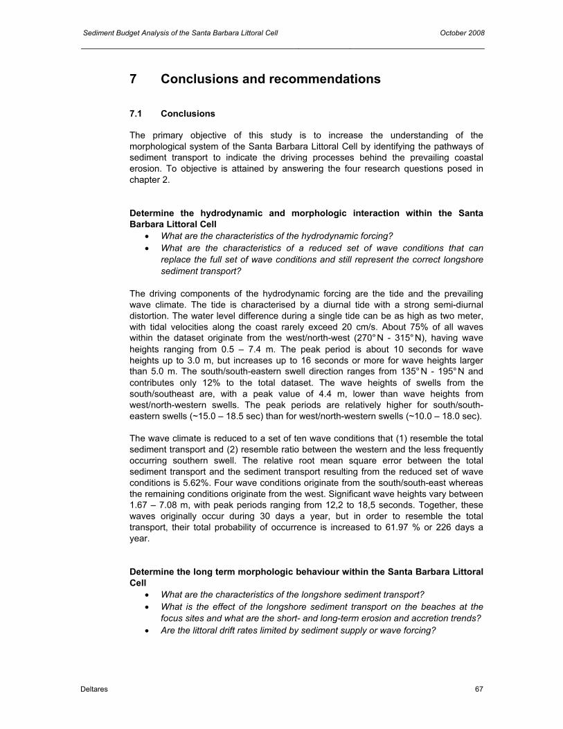
Sediment Budget Analysis of the Santa Barbara Littoral Cell October 2008
Deltares 67
7 Conclusions and recommendations
7.1 Conclusions
The primary objective of this study is to increase the understanding of the morphological system of the Santa Barbara Littoral Cell by identifying the pathways of sediment transport to indicate the driving processes behind the prevailing coastal erosion. To objective is attained by answering the four research questions posed in chapter 2. Determine the hydrodynamic and morphologic interaction within the Santa Barbara Littoral Cell
• What are the characteristics of the hydrodynamic forcing? • What are the characteristics of a reduced set of wave conditions that can
replace the full set of wave conditions and still represent the correct longshore sediment transport?
The driving components of the hydrodynamic forcing are the tide and the prevailing wave climate. The tide is characterised by a diurnal tide with a strong semi-diurnal distortion. The water level difference during a single tide can be as high as two meter, with tidal velocities along the coast rarely exceed 20 cm/s. About 75% of all waves within the dataset originate from the west/north-west (270°N - 315°N), having wave heights ranging from 0.5 – 7.4 m. The peak period is about 10 seconds for wave heights up to 3.0 m, but increases up to 16 seconds or more for wave heights larger than 5.0 m. The south/south-eastern swell direction ranges from 135°N - 195°N and contributes only 12% to the total dataset. The wave heights of swells from the south/southeast are, with a peak value of 4.4 m, lower than wave heights from west/north-western swells. The peak periods are relatively higher for south/south-eastern swells (~15.0 – 18.5 sec) than for west/north-western swells (~10.0 – 18.0 sec). The wave climate is reduced to a set of ten wave conditions that (1) resemble the total sediment transport and (2) resemble ratio between the western and the less frequently occurring southern swell. The relative root mean square error between the total sediment transport and the sediment transport resulting from the reduced set of wave conditions is 5.62%. Four wave conditions originate from the south/south-east whereas the remaining conditions originate from the west. Significant wave heights vary between 1.67 – 7.08 m, with peak periods ranging from 12,2 to 18,5 seconds. Together, these waves originally occur during 30 days a year, but in order to resemble the total transport, their total probability of occurrence is increased to 61.97 % or 226 days a year. Determine the long term morphologic behaviour within the Santa Barbara Littoral Cell
• What are the characteristics of the longshore sediment transport? • What is the effect of the longshore sediment transport on the beaches at the
focus sites and what are the short- and long-term erosion and accretion trends? • Are the littoral drift rates limited by sediment supply or wave forcing?

October 2008 Sediment Budget Analysis of the Santa Barbara Littoral Cell
68 Deltares
The longshore sediment transport is reflected by the residual current, which accounts for the combined effect of the tidal and littoral current. The residual current, and consequently the longshore sediment transport, is almost uniformly directed from west to east/southeast. Changes in coastline orientation (either abrupt or gradual) and alongshore water depth variations, results in significant longshore sediment transport gradients. Although the net sediment transport is almost unidirectional from west to east, there is a distinct difference in the composition of the sediment transport rates between the coastline upcoast (transect 10-15) and downcoast (transect 16-28) of Sandyland. While hardly affected by southern swell, gross transports are negligible along the coastline west of Sandyland. Downcoast of Sandyland the gross sediment transport rates are, although dominated by western swell, significantly higher because of the effect of southern swell on the sediment transport. The simulated longshore sediment transport rates are in good agreement with the annual dredging rates at the Santa Barbara and Ventura Harbor. The error between the simulated littoral drift rates and the dredging rates is in the order of 10%, with the simulated transport rates being underestimated. Based on the analysis of the simulated residual current the main characteristics of the littoral drift rates at the focus sites within the Santa Barbara Littoral Cell can be summarized as:
• Goleta region: the abrupt counter clockwise rotation of the coastline at the western side of Ellwood Beach locally increases the residual velocities. Halfway Ellwood Beach, the coastline bends back in seaward direction and the velocities decrease up to Devereux Slough. Consequently, erosion occurs at the western part of Ellwood Beach, whereas the eastern side of the beach in front of the Devereux Slough accretes. While seeking for equilibrium, the beach rotates clockwise and disappears around the rocks at Coal Oil Point. Isla Vista Beach shows a similar clockwise rotation. Sediment is being transported from west to east, where the residual velocities are decreased and accretion occurs. The lack of sediment being transported around the cliff at Coal Oil Point results in an ongoing reduction of the beach volume. Just downcoast of Goleta point, the decline in the residual velocities suggest an accreting trend at UCSB and the western side of Goleta Beach. The lack of sediment being transported around Campus Point however prevents the beaches of UCSB and the part of Goleta Beach west to Goleta Slough to accrete. East of Goleta slough, the residual current increases and is dominated by western swell, resulting in an eroding trend of Goleta Beach. The sediment transport at this part of the coastline is dominated by the frequently occurring wave condition 24.
• Carpinteria region: there is a long-term trend of erosion at the City of Carpinteria Beach and accretion at the eastern side of Carpinteria state Beach. The revetment along the coastline directly upcoast of the City of Carpinteria Beach and along Sandyland, maintains the erosion at the City of Carpinteria Beach. While the revetment prevents erosion at Sandyland and fixates Sandy Point, rotation of the coastline (i.e. reducing the angle of wave approach) is restricted to the beaches in front of Carpinteria. The fixation of Sandyland prevents the adaptation of the coastline to the prevailing wave condition and maintains the relative large angle of wave approach of western swells.
• Ventura Harbor region: Gross sediment transport rates are large in this region because of the orientation of the southwest facing coastline: swells, coming from either the west or the south, have maximum impact on the sediment transport while the angle of wave approach is in the order of 45° for both
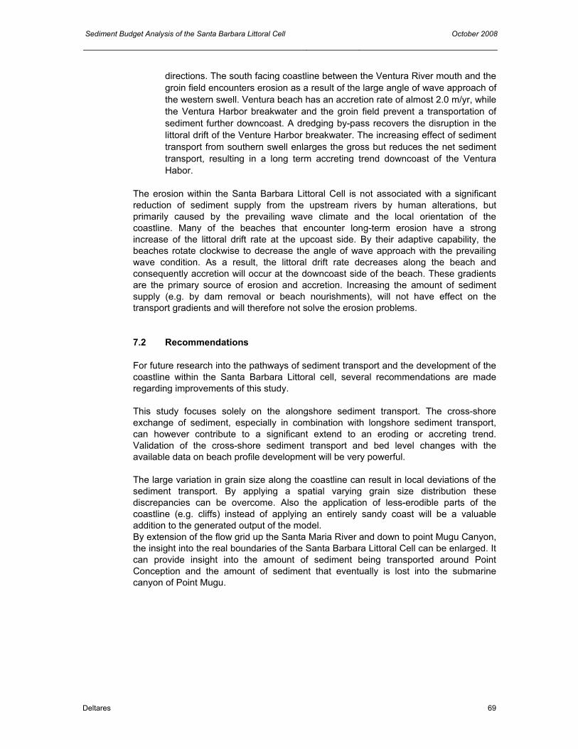
Sediment Budget Analysis of the Santa Barbara Littoral Cell October 2008
Deltares 69
directions. The south facing coastline between the Ventura River mouth and the groin field encounters erosion as a result of the large angle of wave approach of the western swell. Ventura beach has an accretion rate of almost 2.0 m/yr, while the Ventura Harbor breakwater and the groin field prevent a transportation of sediment further downcoast. A dredging by-pass recovers the disruption in the littoral drift of the Venture Harbor breakwater. The increasing effect of sediment transport from southern swell enlarges the gross but reduces the net sediment transport, resulting in a long term accreting trend downcoast of the Ventura Habor.
The erosion within the Santa Barbara Littoral Cell is not associated with a significant reduction of sediment supply from the upstream rivers by human alterations, but primarily caused by the prevailing wave climate and the local orientation of the coastline. Many of the beaches that encounter long-term erosion have a strong increase of the littoral drift rate at the upcoast side. By their adaptive capability, the beaches rotate clockwise to decrease the angle of wave approach with the prevailing wave condition. As a result, the littoral drift rate decreases along the beach and consequently accretion will occur at the downcoast side of the beach. These gradients are the primary source of erosion and accretion. Increasing the amount of sediment supply (e.g. by dam removal or beach nourishments), will not have effect on the transport gradients and will therefore not solve the erosion problems. 7.2 Recommendations
For future research into the pathways of sediment transport and the development of the coastline within the Santa Barbara Littoral cell, several recommendations are made regarding improvements of this study. This study focuses solely on the alongshore sediment transport. The cross-shore exchange of sediment, especially in combination with longshore sediment transport, can however contribute to a significant extend to an eroding or accreting trend. Validation of the cross-shore sediment transport and bed level changes with the available data on beach profile development will be very powerful. The large variation in grain size along the coastline can result in local deviations of the sediment transport. By applying a spatial varying grain size distribution these discrepancies can be overcome. Also the application of less-erodible parts of the coastline (e.g. cliffs) instead of applying an entirely sandy coast will be a valuable addition to the generated output of the model. By extension of the flow grid up the Santa Maria River and down to point Mugu Canyon, the insight into the real boundaries of the Santa Barbara Littoral Cell can be enlarged. It can provide insight into the amount of sediment being transported around Point Conception and the amount of sediment that eventually is lost into the submarine canyon of Point Mugu.


Sediment Budget Analysis of the Santa Barbara Littoral Cell October 2008
Deltares 71
8 References
Barnard P.L. (2006) “Field Santa Barbara and Ventura Counties Coastal Processes Study – Interim Progress Report to BEACON, 14 p.
Barnard P.L. et al. (2007) “Field Test Comparison of an Autocorrelation Technique for
Determining Grain Size using a Digital Beachball Camera versus Traditional Methods”. Sedimentary Geology 201, 180-195.
Barnard P.L. et al. (2007) “Carpinteria Coastal Processes Study, 2005-2007; Final
Report”. U.S. Geological Survey, Open-File Report 2007 – 1412, 129 p. Battjes J., Stive M.J.F. (1985) “Calibration and Verification of a Dissipation Model for
Random Breaking Waves”. Journal of Geophysical Research, Volume 90, No C5, 9159-9167.
California Department of Boating and Waterways and State Coastal Conservancy
(2002) “California Beach Restoration Study”. Sacramento, California. http://www.dbw.ca.gov/PDF/Reports/BeachReport/FrontMatter.pdf
California Rivers Assessment (1992) California Resources Agency,
http://endeavor.des.ucdavis.edu/newcara/ Booij N. et al. (1999) “A Third-generation Wave Model for Coastal Regions, Part 1,
Model Description and Validation”. Journal of Geophysical Research, Volume 104, No. C4, 7649-7666.
ENTRIX, INC. (2002) “Resident Species Study Santa Clara River Estuary; Ventura
Water Reclamation Facility NPDES Permit No. CA0053651, CI-1822”. Ventura, California, City of San Buenavuerta.
Gallapatti, R. (1983) “A Depth Integrated Model for Suspended Transport”. Report 83-
7, Communications on Hydraulics, Department of Civil Engineering, Delft University of Technology.
Inman, D.L. and Masters, P.M. (1991) “Coastal Sediment Transport Concepts and
Mechanisms”, Chapter 5 in State of the Coast Report, San Diego Region, Coast of California Storm and Tidal Waves Study, U.S. Army Corps of Engineers, Los Angeles District, Chapters 1-10.
Hapke C.J. et al. (2006) “National Assessment of Shoreline Change: Part 3: Historical
Shoreline Changes and Associated Coastal Land Loss along the Sandy Shorelines of the California Coast”. U.S. Geological Survey Open-file Report 2006-1219.
Hapke C.J. and Reid, D. (2007) “National Assessment of Shoreline Change: Part 4:
Historical Coastal Cliff Retreat along the California Coast”. U.S. Geological Survey Open-file Report 2007-1133.

October 2008 Sediment Budget Analysis of the Santa Barbara Littoral Cell
72 Deltares
Henson P. and Usner, D.J. (1996) “The Natural History of Bug Sur”, University of California Press, ISBN 0520205103
Hickey, B.M. (1992) “Circulation over the Santa Monica-San Pedro Basin and Shelf”,
Progress in Oceanography, Volume 30, 37-115. Holthuijsen L.H. et al. (1993) “A Spectral Wave Model for the Coastal Zone”. Proc. Of
2nd Int. Symposium on Ocean Wave Measurement and Analysis, New Orleans, 630-641.
Holthuijsen L.H. (2007) “Waves in Oceanic and Coastal Waters”. Cambridge
University Press, 1st edition. ISBN-13 978-0-521-86028. Latteux B. (1995) “Techniques for Long-term Morphological Simulation under Tidal
Action”. Marine Geology, Volume 126, 129-141. Lesser G. et al. (2000) “Online Sediment Transport within Delft3D-FLOW”. Report Z
2899, WL|Delft Hydraulics, The Netherlands. Lesser G. et al. (2004) “Development and Validation of a Three-dimensional
Morphological Model”. Coastal Engineering 51, 883-915. Münchow, A. (1997) “Tidal Currents in a Topographically Complex Channel”,
Continental Shelf Research 18, 561-584. Mustain N.M. (2007) “Grain Size Distribution of Beach and Nearshore Sediments of the
Santa Barbara Littoral Cell: Implications for Beach Nourishment”. M.Sc. Thesis, University of California, Santa Cruz, 107 p.
Patsch K.B. (2004) “An Analysis of Littoral Cell Sand Budgets for California
[Dissertation]”. University of California, Santa Cruz, 174 p. Patsch K.B., Griggs G.B. (2006) “Littoral Cells, Sand Budgets and Beaches:
Understanding California’s Shoreline”. Institute of Marine Sciences, University of California, Santa Cruz, 40 p.
Patsch K.B., Griggs G.B. (2007) “Development of Sand Budgets for California’s Major
Littoral Cells”. Institute of Marine Sciences, University of California, Santa Cruz, 115 p.
Revell D.L. amd Griggs G.B. (2005) “Long-term and Storm Event Changes to the
Beaches of Isla Vista, California”. Institute of Marine Sciences, University of California, Santa Cruz, 23 p, http://spf.as.ucsb.edu/shoreline_change.pdf
Roelvink, J.A., Walstra D.J.R. (2004) “Keeping it Simple by using Complex Models”.
6th International Conference on Hydroscience and Engineering, Advances in Hydro-Science and -Engineering, Brisbane, Australia.
Runyan K.B., Griggs G.B. (2003) “The Effects of Armoring Seacliffs on the Natural
Sand Supply to the Beaches of California”. Journal of Coastal Research 19(2): 336-347.

Sediment Budget Analysis of the Santa Barbara Littoral Cell October 2008
Deltares 73
Stillwater Sciences (2007) “Santa Clara River Parkway Floodplain Restoration Feasibility Study: Assessment of Geomorphic Processes for the Santa Clara River Watershed, Ventura and Los Angeles Counties, California.
Steijn, R.C. (1989) “Voordelta Morphological Study: Schematisation of the Natural
Conditions in Multi-dimensional Numerical Models of Coastal Morphology”. Report H 526, WL|Delft Hydraulics, The Netherlands.
Steijn, R.C. (1992) “Input Filtering Techniques for Complex Morphological Models”.
Report H 824.65, WL|Delft Hydraulics, The Netherlands. Van de Graaf, J. (2006) “Coastal Morphology and Coastal Protection- Lecture notes”,
Deltf University of Technology, The Netherlands. Van Rijn, L.C. (1985) “Two-dimensional Vertical Mathematical Model for Suspended
Sediment Transport by Currents and Waves”. Report S0488, Part IV, WL|Delft Hydraulics, Delft, The Netherlands.
Van Rijn, L.C. (2000) “General View on Sand Transport by Currents and Waves”.
Report Z2899.20-Z2099.30-Z2824.30, WL|Delft Hydraulics, Delft, The Netherlands.
Van Rijn, L.C., Walstra D.J.R. (2003) “Modelling of Sand Transport in Delft3D-Online”.
Report Z 3624, WL|Delft Hydraulics, The Netherlands. Warrick J.A. (2002) “Short-term (1997-2002) and Long-term (1928-2000) Observations
of River Water and Sediment Discharge to the Santa Barbara Channel, Ph.D. thesis, University of California, Santa Barbara, 337 p.
Warrick J.A. et al. (2003) “Hyperpycnal Sediment Discharge from Semiarid Southern
California Rivers: Implications for Coastal Sediment Budgets”. Geology 31 (9), 781-784.
Warrick J.A. et al. (2004) “A Conceptual Model for River Water and Sediment
Dispersal in the Santa Barbara Channel, California”. Continental Shelf Research 24, 2029-2043.
Williams, R.P. (1979) “Sediment Discharge in the Santa Clara River Basin, Ventura
and Los Angeles Counties, California”. U.S. Geological Survey, Menlo Park, California.
WL|Delft Hydraulics (2006) “Delft3D-FLOW Manual Version 3.13, Simulation of Multi-
dimensional Hydrodynamic Flows and Transport Phenomena, Including Sediments”. Delft, The Netherlands.
WL|Delft Hydraulics (2006) “Delft3D-WAVE Manual Version 3.03, Simulation of Short-
crested Waves with SWAN”. Delft, The Netherlands. WL|Delft Hydraulics (2007) “Schematisation of Boundary Conditions for Morphological Simulations - unpublished report”, Delft, The Netherlands.


Sediment Budget Analysis of the Santa Barbara Littoral Cell October 2008
Deltares 75
A Governing equations Delft3D FLOW and WAVE
A.1 Modelling of the hydrodynamics (Delft3D-FLOW) This section about the FLOW module is partially taken from the Delft3D-FLOW User Manual (WL| Delft Hydraulics, 2006). The FLOW module solves the non-linear shallow water equations, which are derived from the three dimensional Navier Stokes equations for incompressible free surface flow, in two (depth-averaged) or three dimensions. The system of equations consists of the horizontal momentum equations, the continuity equation and the transport equations. While the water depth is assumed to be much smaller than the horizontal length scale, the shallow water assumption is valid. Under this assumption the vertical momentum equation can be reduced to the hydrostatic pressure equation. The vertical accelerations are assumed to be small compared to the gravitational acceleration and are therefore not taken into account. The system of equations that are used in the FLOW module take the following processes into account:
- Tidal forcing - Free surface gradients (barotropic effects) - The effect of the Earth’s rotation (Coriolis force) - Tidal potential (tide generating forces) - Water with variable density - Horizontal density gradients in pressure (baroclinic effects) - Turbulence induced mass and momentum fluxes - Transport of salt, heat and other conservative elements - Space and time varying wind shear stress on the water surface - Bed shear stress on the base of the flow - Space and time varying atmospheric pressure on the water surface - Time varying sources and sinks (e.g. river discharges) - Drying and flooding of tidal flats - Lateral shear stress due to rough walls - Effects of secondary flow on depth averaged momentum equations - Influence of surface waves on the bed shear stress - Wave induced stresses and mass fluxes
To solve the partial differential equations in a numerical model, the equations should be transformed to a discrete space. In the Delft3D-FLOW module a finite difference scheme on a staggered rectangular or curvilinear grid is chosen to approximate these equations. For each grid cell within this staggered grid, Delft3D calculates both the water level and the velocity. The water level points are defined in the centre of a grid cell, while the velocity components are perpendicular to the grid cell boundaries (Fig. A.1).
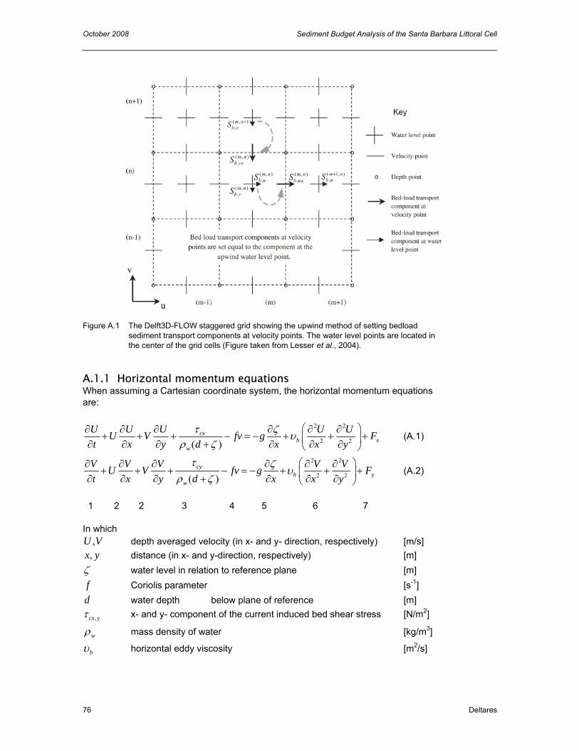
October 2008 Sediment Budget Analysis of the Santa Barbara Littoral Cell
76 Deltares
Figure A.1 The Delft3D-FLOW staggered grid showing the upwind method of setting bedload
sediment transport components at velocity points. The water level points are located in the center of the grid cells (Figure taken from Lesser et al., 2004).
A.1.1 Horizontal momentum equations When assuming a Cartesian coordinate system, the horizontal momentum equations are:
2 2
2 2( )cx
h xw
U U U U UU V fv g Ft x y d x x y
τ ζ υρ ζ
⎛ ⎞∂ ∂ ∂ ∂ ∂ ∂+ + + − = − + + +⎜ ⎟∂ ∂ ∂ + ∂ ∂ ∂⎝ ⎠
(A.1)
2 2
2 2( )cy
h yw
V V V V VU V fv g Ft x y d x x y
τ ζ υρ ζ
⎛ ⎞∂ ∂ ∂ ∂ ∂ ∂+ + + − = − + + +⎜ ⎟∂ ∂ ∂ + ∂ ∂ ∂⎝ ⎠
(A.2)
1 2 2 3 4 5 6 7 In which
,U V depth averaged velocity (in x- and y- direction, respectively) [m/s] ,x y distance (in x- and y-direction, respectively) [m]
ζ water level in relation to reference plane [m] f Coriolis parameter [s-1] d water depth below plane of reference [m]
,cx yτ x- and y- component of the current induced bed shear stress [N/m2]
wρ mass density of water [kg/m3]
hυ horizontal eddy viscosity [m2/s]

Sediment Budget Analysis of the Santa Barbara Littoral Cell October 2008
Deltares 77
The terms within Eq. (A.1) and (A.2) represent: 1. velocity gradient 5. barotropic pressure gradient 2. advective terms 6. horizontal eddy viscosity 3. bottom stress 7. external forces 4. Coriolis force Both Fx and Fy represent the contributions due to external sources or sinks of momentum (external forces by hydraulic structures, discharge or withdrawal of water, wave stresses, etc.) and are taken from the WAVE simulations:
yxxx xx
SS kF Dx y ω
∂∂= − − =
∂ ∂ (A.3)
xy yy yy
S S kF D
x y ω∂ ∂
= − − =∂ ∂
(A.4)
where S is the radiation stress tensor:
2 2
0 0[ cos 1/ 2]xxS g n n Ed d
πρ θ σ θ
∞= + −∫ ∫ (A.5)
2
0 0sin cosyx xyS S g n Ed d
πρ θ θ θ σ
∞= = ∫ ∫ (A.6)
2 2
0 0[ sin 1/ 2]yyS g n n Ed d
πρ θ σ θ
∞= + −∫ ∫ (A.7)
In which
,x yF radiation stress gradient in x- and y- direction, respectively [N/m2]
xxS radiation stress [N/m]
D total energy dissipation due to waves [N/ms] ,x yk k wave number [m-1]
ω wave frequency [s-1] The bottom shear stress in Eq. (A.1) and (A.2) induced by the flow can be defined in several ways. For depth averaged flow (2D) the shear stress on the bed may be computed by various types of formulations like Chèzy, Manning or White Colebrook and can be written in the form:
2cx w
U ug
Cτ ρ
⎛ ⎞= ⎜ ⎟
⎝ ⎠
v
In which U is the absolute magnitude of depth-averaged horizontal velocity and C
represents the Chèzy coefficient.
October 2008 Sediment Budget Analysis of the Santa Barbara Littoral Cell
78 Deltares
A.1.2 Continuity equations The depth-averaged continuity equation is given by
[( ) ] [( ) ] 0d U d Vt x yζ ζ ζ∂ ∂ + ∂ ++ + =
∂ ∂ ∂ (A.8)
1 2 3 In which ζ water level in relation to reference plane [m]
,x y distance (in x- and y-direction, respectively) [m] t time [s] d water depth below plane of reference [m]
,U V depth averaged velocity (in x- and y- direction, respectively) [m/s] The terms within Eq. (A.8) represent: 1. water level gradient as a function of the time 2. specific discharge gradient in x-direction 3. specific discharge gradient in y-direction
A.1.3 Transport equations The FLOW module makes alternating calls to the sediment transport and morphology modules at each time step. The modules enable the calculation of both suspended and bed load transport for non-cohesive as well as cohesive sediments. The suspended load transport is based on the numerical solution of the depth-integrated advection-diffusion equation:
2 2
2 2
( ) ( ) ( ) ( ) ( ) eqh h
s
c chc hc hc hc hcu v D D ht x y x y T
−∂ ∂ ∂ ∂ ∂+ + − − =
∂ ∂ ∂ ∂ ∂ (A.9)
In which h water depth [m]
,u v depth averaged velocity (in x- and y- direction, respectively) [m/s]
hD horizontal dispersion coefficient [m2/s]
sT adaptation time-scale [s] c depth averaged concentration [kg/m3] The depth averaged equilibrium concentration eqc is defined as:
,s eq
eq
Sc
u h=
ur
r (A.10)
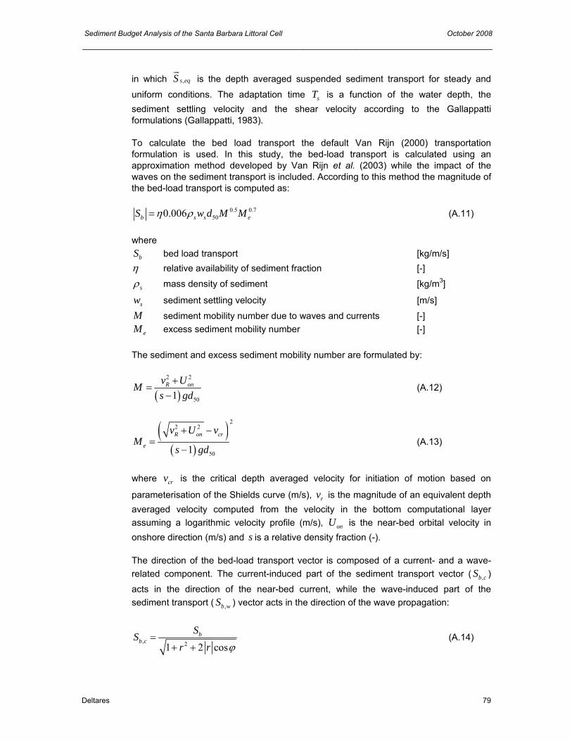
Sediment Budget Analysis of the Santa Barbara Littoral Cell October 2008
Deltares 79
in which ,s eqSur
is the depth averaged suspended sediment transport for steady and
uniform conditions. The adaptation time sT is a function of the water depth, the sediment settling velocity and the shear velocity according to the Gallappatti formulations (Gallappatti, 1983). To calculate the bed load transport the default Van Rijn (2000) transportation formulation is used. In this study, the bed-load transport is calculated using an approximation method developed by Van Rijn et al. (2003) while the impact of the waves on the sediment transport is included. According to this method the magnitude of the bed-load transport is computed as:
0.5 0.7500.006b s s eS w d M Mη ρ= (A.11)
where
bS bed load transport [kg/m/s] η relative availability of sediment fraction [-]
sρ mass density of sediment [kg/m3]
sw sediment settling velocity [m/s]
M sediment mobility number due to waves and currents [-]
eM excess sediment mobility number [-] The sediment and excess sediment mobility number are formulated by:
( )2 2
501R onv UM
s gd+
=−
(A.12)
( )( )
22 2
501R on cr
e
v U vM
s gd
+ −=
− (A.13)
where crv is the critical depth averaged velocity for initiation of motion based on
parameterisation of the Shields curve (m/s), rv is the magnitude of an equivalent depth averaged velocity computed from the velocity in the bottom computational layer assuming a logarithmic velocity profile (m/s), onU is the near-bed orbital velocity in onshore direction (m/s) and s is a relative density fraction (-). The direction of the bed-load transport vector is composed of a current- and a wave-related component. The current-induced part of the sediment transport vector ( ,b cS )
acts in the direction of the near-bed current, while the wave-induced part of the sediment transport ( ,b wS ) vector acts in the direction of the wave propagation:
, 21 2 cosb
b cSS
r r ϕ=
+ + (A.14)

October 2008 Sediment Budget Analysis of the Santa Barbara Littoral Cell
80 Deltares
, ,b w b cS r S= (A.15)
in which:
( )( )
3
3on cr
r cr
U vr
v v
−=
− (A.16)
This implies that , 0b wS = if 0.01r < and , 0b cS = if 100r > . The angle between
current and wave direction is defined by ( )ϕ and is suggested to be a constant value of
ninety degrees. The suspended sediment transport that results from wave asymmetry is also included in the bed-load transport vector by using an approximation method proposed by Van Rijn (2001):
,s w A TS U Lγ= (A.17)
where
,s wS = wave-related suspended transport [kg/m/s]
γ = phase lag coefficient [-]
AU = velocity asymmetry value [m/s]
TL = suspended sediment load = 500.007 s ed Mρ [kg/m2] The velocity asymmetry AU is determined by:
4 4
3 3on off
Aon off
U UU
U U⎛ ⎞−
= ⎜ ⎟⎜ ⎟−⎝ ⎠
The direction of the current induced bed-load ,b cS is assumed to be equal to the
direction of the current, while the wave related transport components ,b wS and ,s wS acts
in the direction of the wave propagation.

Sediment Budget Analysis of the Santa Barbara Littoral Cell October 2008
Deltares 81
A.2 Modelling of the waves (Delft3D-WAVE) This section about the Delft3D-WAVE module (version 4.91.02) is partially taken from the Delft3D-WAVE User Manual (WL| Delft Hydraulics, 2006). In this module the third-generation SWAN model (version 40.51A) is implemented, that accounts for refraction, propagation, wave-wave interaction, wind-induced wave growth bottom dissipation, depth induced wave breaking and current breaking (Holthuijsen et al., 1993). The waves are described with the two-dimensional wave action density spectrum N(σ,θ) rather than the energy density spectrum E(σ,θ), since in the presence of currents the action density is preserved whereas energy density is not. The action density is equal to the energy density E(σ,θ) divided by the relative frequency (σ):
( , )( , ) EN σ θσ θσ
= (A.18)
In SWAN the evolution of the wave spectrum is described by the spectral action balance equation, which for Cartesian coordinates is formulated as:
, ,( , ) ( , ) ( , ) ( , )( , ) ( , )g x g yc N c N c N c NN St x y
θ σσ θ σ θ σ θ σ θσ θ σ θ
θ σ σ∂ ∂ ∂ ∂∂
+ + + + =∂ ∂ ∂ ∂ ∂
(A.19)
In which
( , )N σ θ Wave action density ( , )E σ θ Energy density ,x y Distance (in x- and y-direction, respectively) [m]
, , ,x yc σ θ Propagation speed for x, y, σ, θ, respectively [m/s]
σ Relative frequency [Hz] θ Wave direction [degrees]
( , )S σ θ Source/sink term in terms of energy density The first term on the left-hand side of Eq. (A.19) represents the local rate of change of action in time, the second and third terms represent propagation of action in geographic space (with propagation velocities cg,x and cg,y in x- and y-space, respectively). The fourth term represents depth- and current-induced refraction (with propagation velocity cθ in θ-space), while the fifth term represents the shifting of the relative frequency due to variations in depths and currents. The term S at the right-hand side of the action balance equation is the source term in terms of energy density representing the effects of generation, dissipation and non-linear wave-wave interaction. The integration of the action balance equation Eq. (A.19) has been implemented in SWAN with a implicit upwind scheme.


Sediment Budget Analysis of the Santa Barbara Littoral Cell October 2008
Deltares 83
B Conceptual description Opti-Routine
Initial weights
Target
New weights
RMS of diff(WAD,target
Take weights of iteration for which applies:
WAD
Iterationloop
Assign random weights to close
conditions
Determine most-closely correlated conditions
(close conditions)
Elimination
loop
Determine contribution of each condition to
target with new weights
Eliminate condition with lowest contribution (set weight to zero)
Data
Only 1 condition left
The diagram shows that during each elimination step, the iteration loop is performed, also for the first elimination step, with all conditions participating. During this step no conditions are eliminated yet, there are no most-closely correlated conditions to assign random weight to, so in fact nothing happens during this iteration loop. The weights from the iteration loop during the first step of the elimination loop are equal to the initial weights.


Sediment Budget Analysis of the Santa Barbara Littoral Cell October 2008
Deltares 85
C Tables
Table C.1.1 Tidal datums (period: 1991-1997). Source: http://tidesandcurrents.noaa.gov
TIDAL DATUMS
Tidal datums at SANTA BARBARA, PACIFIC OCEAN based on:
LENGTH OF SERIES : 7 years
TIME PERIOD : januari 1991 – December 1997
TIDAL EPOCH : 1983 – 2001
CONTROL TIDE STATION : 9410660 LOS ANGELOS, OUTER HARBOR
Elevations of tidal datums referred to Mean Lower Low Water (MLLW), in METERS:
HIGHEST OBSERVED WATER LEVEL (01/19/1992) : 2.242
MEAN HIGHER HIGH WATER (MHHW) : 1.643
MEAN HIGH WATER (MHW) : 1.413
MEAN TIDE LEVEL (MTL) : 0.856
MEAN SEA LEVEL (MSL) : 0.850
MEAN LOW WATER (MLW) : 0.300
NORTH AMERICAN VERTICAL DATUM-1998 (NAVD) : 0.029
MEAN LOWER LOW WATER (MLLW) :0.000
LOWEST OBSERVED WATER LEVEL (12/17/1993) : -0.892
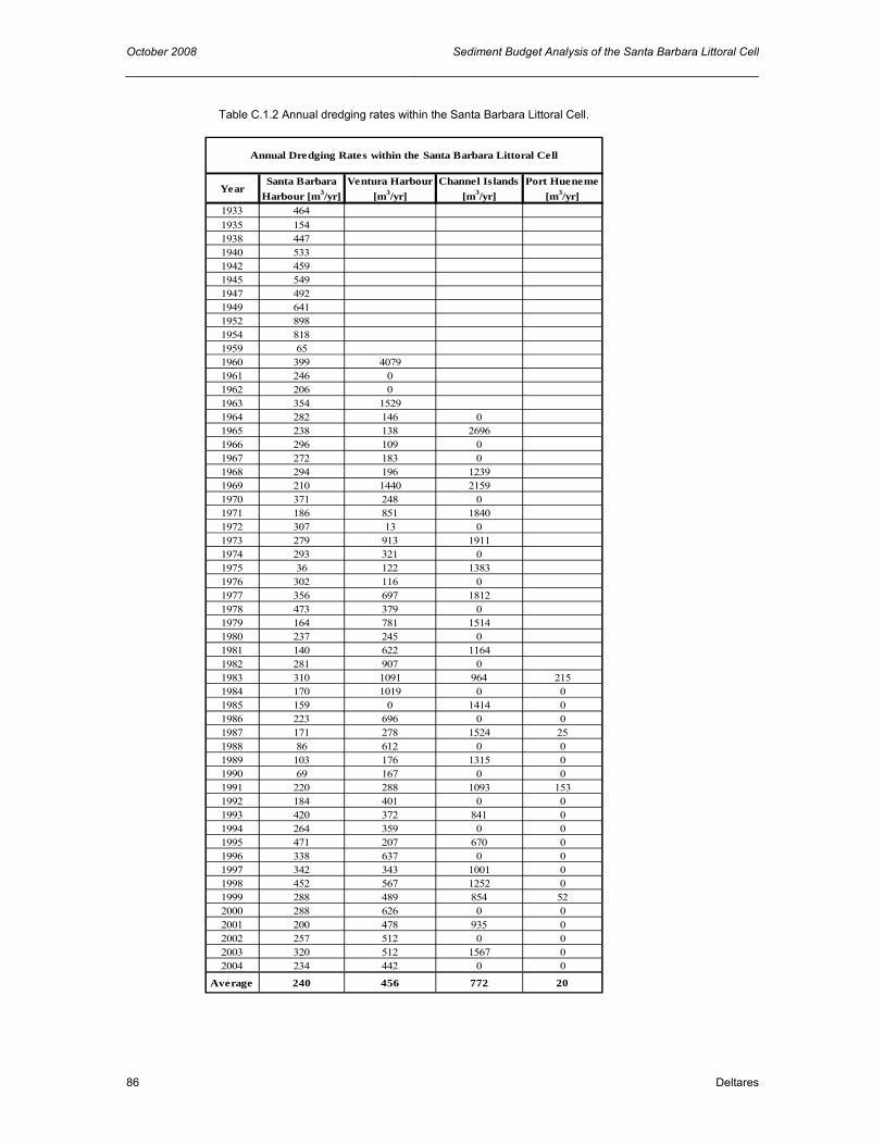
October 2008 Sediment Budget Analysis of the Santa Barbara Littoral Cell
86 Deltares
Table C.1.2 Annual dredging rates within the Santa Barbara Littoral Cell.
YearSanta Barbara
Harbour [m3/yr]Ventura Harbour
[m3/yr]Channel Islands
[m3/yr]Port Hueneme
[m3/yr]1933 4641935 1541938 4471940 5331942 4591945 5491947 4921949 6411952 8981954 8181959 651960 399 40791961 246 01962 206 01963 354 15291964 282 146 01965 238 138 26961966 296 109 01967 272 183 01968 294 196 12391969 210 1440 21591970 371 248 01971 186 851 18401972 307 13 01973 279 913 19111974 293 321 01975 36 122 13831976 302 116 01977 356 697 18121978 473 379 01979 164 781 15141980 237 245 01981 140 622 11641982 281 907 01983 310 1091 964 2151984 170 1019 0 01985 159 0 1414 01986 223 696 0 01987 171 278 1524 251988 86 612 0 01989 103 176 1315 01990 69 167 0 01991 220 288 1093 1531992 184 401 0 01993 420 372 841 01994 264 359 0 01995 471 207 670 01996 338 637 0 01997 342 343 1001 01998 452 567 1252 01999 288 489 854 522000 288 626 0 02001 200 478 935 02002 257 512 0 02003 320 512 1567 02004 234 442 0 0
Average 240 456 772 20
Annual Dredging Rates within the Santa Barbara Littoral Cell

Sediment Budget Analysis of the Santa Barbara Littoral Cell October 2008
Deltares 87
Table C.3.1 Summary of the main model parameters applied in the Delft3D model Module Parameter Value Description
FLOW ∆t 30 Flow time step [s]g 9.81 Gravitational acceleration factor [m/s2]ρw 1025 Water density [kg/m3]Vicouv 1.0 Horizontal eddy viscosity [m2/s]Dicouv 1.0 Horizontal eddy diffusivity [m2/s]Bottom roughness Chezy Roughness formulaCcofu 65 Chezy friction coefficient in U-direction [-]Ccofv 65 Chezy friction coefficient in V-direction [-]Dryflc 0.1 Threshold depth of drying and flooding [m]Dco -999 Marginal depth in shallow areas [m]
WAVE Bathymetry 1 Use bathymetry from FLOW computation [-]Water level 1 Use water level from FLOW computation [-]Current 1 Use current from FLOW computation [-]Wind 1 Use wind from FLOW computation [-]Directional space 360 Sector, counterclockwise w.r.t. North [°]
72 Number of spectral directions [-]Frequency space 0.02 Lowest frequency [1/s]
0.5 Highest frequency [1/s]24 Number of frequency bins [-]
Spectral space JONSWAP Shape of the spectrumpeak Period3.3 Peak enhancement factor for JONSWAP spectrum [-]10 Directional spreading
Boundary conditions Unifom Type of boundary conditionParametric Specification of spectrum
Set-up FALSE Wave related set-upForcing radiation stress Computation of wave forcesGeneration mode 3rd Generation mode for physicsWave breaking B&J model Depth-induced breaking model
1 Coefficient for wave energy dissipation [-]0.73 Breaker parameter [-]
Troads (LTA) FALSE Non-linear wave-wave interactionBottom friction JONSWAP Bottom friction formulation
0.038 Bottom friction coefficient [m2/s3]Diffraction FALSE Formulation for diffractionWind growth FALSE Formulation for exponentional wave growthWhite capping TRUE Formulation for white cappingQuadruplets FALSE Quadruplet wave-wave interactionRefraction TRUE Refraction for wave propagation in spectral spaceFrequency shift TRUE Frequency shift for wave propagation in spectral space
MOR MorFac 1 Morphological scaling factor [-]Morstt 10 Spin-up interval for morphological changes [min]Tresh 0.05 Threshold sediment thickness for transport and erosion reduction [m]EqmBC TRUE Equilibrium sand concentration profile at ininflow boundariesDensin FALSE Include effect of sediment concentration on fluid densityAksfac 1.0 van Rijn's reference height (Aksfac * ks) [-]Rwave 2.0 Wave related roughness (Rwave * estimated ripple height) [-]AlphaBs 1.0 Streamwise bed gradient factor for bed load transport [-]AlphaBn 1.5 Transverse bed gradient factor for bed load transport [-]Sus 1.0 Multiplication factor for suspended sediment reference concentration [-]Bed 1.0 Multiplication factor for bed-load transport vector magnitude [-]SusW 0.0-0.3 Wave related suspended sediment transport factor [-]BedW 0.0-0.3 wave related bed-load sediment transport factor [-]SedThr 0.1 Minimum water depth for sediment computations [m]ThetSD 0.0 Factor for erosion of adjacent dry cellsHMaxTH 1.5 Maximum depth for variable ThetSD [m]FWFac 1.0 Vertical mixing distribution according to van Rijn [-]

October 2008 Sediment Budget Analysis of the Santa Barbara Littoral Cell
88 Deltares
Table C.4.1Prevailing wave climate in the Santa Barbara Channel. The reduced set of wave conditions
consists of those wave conditions indicated in red.
Condition Hs [m] Tp [s] Dir [°] Prob. of occ. [%]
Condition Hs [m] Tp [s] Dir [°] Prob. of occ. [%]
1 1.30 15.36 131 0.05 51 2.77 13.45 334 0.172 1.29 15.40 146 0.25 52 3.02 14.81 140 0.013 1.29 15.36 160 0.67 53 3.42 17.39 153 0.014 1.29 15.06 174 1.82 54 3.36 18.67 173 0.075 1.28 14.87 188 2.34 55 3.22 11.99 266 0.066 1.24 14.98 206 2.16 56 3.25 13.94 280 0.587 1.26 14.39 232 0.29 57 3.24 12.52 294 2.988 1.20 12.71 248 0.5 58 3.23 12.38 306 1.89 1.27 12.56 264 1.19 59 3.25 11.50 322 0.8
10 1.28 12.25 279 2.86 60 3.27 12.21 334 0.0611 1.30 11.10 293 4.72 61 3.76 18.63 158 0.0812 1.30 10.15 307 3.51 62 3.75 18.53 170 0.0913 1.32 10.31 320 0.89 63 3.95 18.50 187 0.0314 1.35 8.89 334 0.04 64 3.67 19.05 217 0.0115 1.65 17.04 125 0.08 65 3.69 17.39 239 0.0116 1.77 14.95 143 0.23 66 3.75 16.00 255 0.0117 1.69 15.32 158 0.52 67 3.69 7.14 267 0.0118 1.67 15.80 173 0.94 68 3.72 14.18 280 0.6319 1.67 15.71 188 1.36 69 3.74 13.12 294 2.1320 1.69 15.57 206 1.23 70 3.69 12.58 306 1.2621 1.70 14.77 233 0.4 71 3.71 11.27 320 0.3322 1.70 13.75 248 0.71 72 3.67 10.81 333 0.0423 1.74 13.64 265 1.57 73 4.11 18.22 161 0.0424 1.74 12.24 279 4.19 74 4.19 17.39 174 0.0125 1.77 10.18 293 10.71 75 4.21 13.73 282 0.126 1.77 10.09 306 5.78 76 4.23 13.22 295 1.1627 1.79 10.36 321 1.44 77 4.22 13.41 306 0.7328 1.76 10.80 333 0.13 78 4.24 11.66 320 0.0829 2.07 15.21 126 0.03 79 4.29 9.14 332 0.0330 2.15 15.49 143 0.09 80 4.69 17.39 270 0.0131 2.21 15.79 160 0.08 81 4.72 14.46 282 0.0532 2.21 15.39 174 0.14 82 4.71 13.72 294 0.6533 2.16 15.91 187 0.21 83 4.73 12.06 305 0.334 2.21 15.34 207 0.17 84 4.74 17.39 318 0.0135 2.24 15.47 237 0.06 85 5.21 16.02 280 0.136 2.23 14.35 249 0.27 86 5.29 13.24 294 0.2737 2.23 14.04 265 0.9 87 5.28 12.17 305 0.1538 2.23 12.79 280 3.54 88 5.71 15.53 278 0.0639 2.25 10.26 294 9.15 89 5.74 12.78 295 0.140 2.24 10.09 306 6.16 90 5.81 11.90 304 0.0241 2.23 10.75 321 1.94 91 6.19 16.32 278 0.0542 2.25 11.32 333 0.09 92 6.18 12.95 295 0.0443 2.65 15.76 176 0.05 93 6.18 13.05 304 0.0444 2.71 13.79 234 0.02 94 6.61 18.22 282 0.0445 2.62 14.47 251 0.03 95 6.61 12.12 288 0.0146 2.72 14.17 265 0.28 96 6.78 13.87 304 0.0347 2.72 13.29 280 1.64 97 7.18 18.03 283 0.0348 2.74 11.06 294 5.06 98 7.27 16.10 293 0.0249 2.71 10.86 306 3.1 99 7.08 14.13 307 0.0350 2.73 11.56 322 1.14

Sediment Budget Analysis of the Santa Barbara Littoral Cell October 2008
Deltares 89
D Wenthworth-Krumbein scale of sediment size
The Wentworth scale divides sediment into size classes based on powers of 2. According to this scale, fine sediment is defined as the clay and silt components and includes all particles smaller than 0.0625 mm in diameter (Table D.1). Krumbein introduced the phi (φ) scale as an alternative measure of sediment size, related to grain size by the equation φ = −log2 d, such that d=2−φ, where d is the grain diameter (in millimeters). Thus, larger phi units correspond to smaller grain sizes.
Sediment size Phy (φ) Lower-bin grain diameter (mm)
Boulder -8 256Cobble -6 64Pebble -2 4Granular -1 2Very course sand 0 1Course sand 1 0.5Medium sand 2 0.25Fine sand 3 0.125Very fine sand 4 0.0625Silt 8 0.004Clay 12 0.00024


Sediment Budget Analysis of the Santa Barbara Littoral Cell October 2008
Deltares 91
E Sensitivity analysis: summary
Using the mean grain size diameter (D50) of 0.26 mm for the entire area results in a realistic pattern of the littoral drift rates, although the dredging rates are underestimated by approximately 50%. The default value of the current-related calibration factors (sus/bed) of 1.0 results in an underestimation of the littoral drift rates upcoast of the Santa Barbara and Ventura Harbor. With respect to the reference simulation, a somewhat higher value of wave-related calibration factors (susw/bedw) will result in a higher correlation between the dredging rates and the sediment transports through transects 12 and 24. With a susw/bedw value of 0.4, a reasonable proxy for the dredging rates is obtained. The result of a simulation with the improved calibration parameters mentioned above is illustrated in Figure E1.1. The Santa Clara and Ventura River discharge is simulated as an average annual discharge. Although underestimated by approximately 20%, the simulated longshore sediment transport appears to be in reasonable agreement with the average dredging data.
Figure E1.1 Littoral drift rates


Sediment Budget Analysis of the Santa Barbara Littoral Cell October 2008
Deltares 93
F Figures

October 2008 Sediment Budget Analysis of the Santa Barbara Littoral Cell
94 Deltares
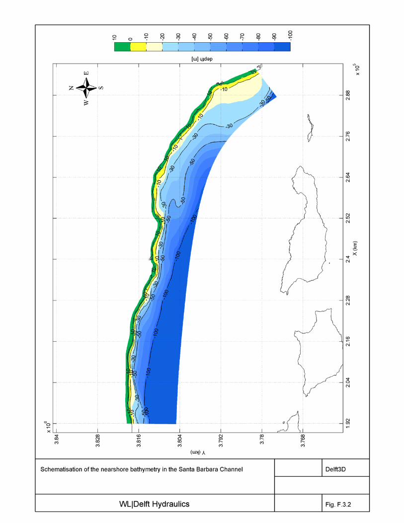
Sediment Budget Analysis of the Santa Barbara Littoral Cell October 2008
Deltares 95
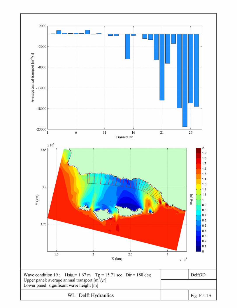
October 2008 Sediment Budget Analysis of the Santa Barbara Littoral Cell
96 Deltares
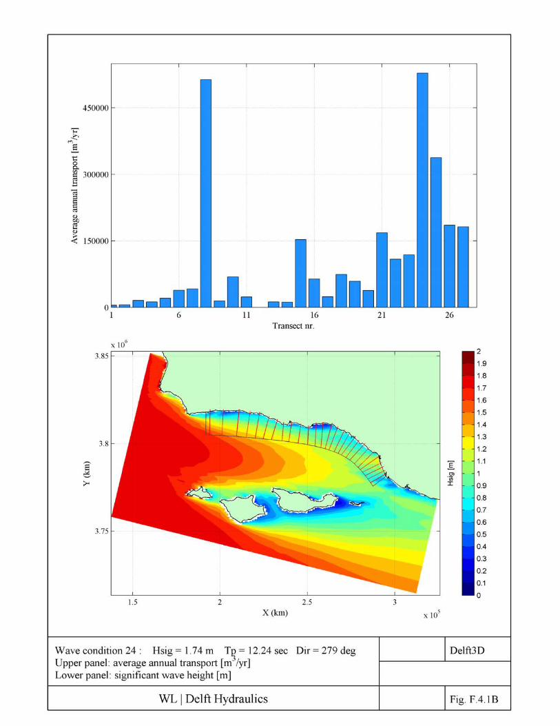
Sediment Budget Analysis of the Santa Barbara Littoral Cell October 2008
Deltares 97

October 2008 Sediment Budget Analysis of the Santa Barbara Littoral Cell
98 Deltares

Sediment Budget Analysis of the Santa Barbara Littoral Cell October 2008
Deltares 99
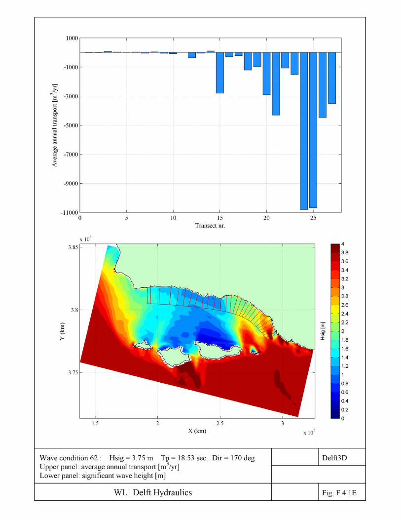
October 2008 Sediment Budget Analysis of the Santa Barbara Littoral Cell
100 Deltares

Sediment Budget Analysis of the Santa Barbara Littoral Cell October 2008
Deltares 101

October 2008 Sediment Budget Analysis of the Santa Barbara Littoral Cell
102 Deltares

Sediment Budget Analysis of the Santa Barbara Littoral Cell October 2008
Deltares 103
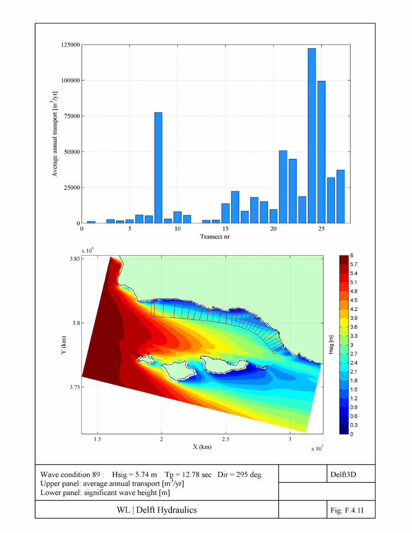
October 2008 Sediment Budget Analysis of the Santa Barbara Littoral Cell
104 Deltares

Sediment Budget Analysis of the Santa Barbara Littoral Cell October 2008
Deltares 105