Apparel and Women’s Wages after the Multi-Fibre … · 5Ley de Inversión Extranejera (Decreto...
32
Apparel and Women’s Wages after the Multi-Fibre Agreement: Evidence from El Salvador Raymond Robertson Macalester College [email protected] Alvaro Trigueros-Argüello FUSADES Preliminary and Incomplete: Please do not quote or cite Version 1.5 June 6, 2011 Keywords: Apparel, Gender, Globalization and Wages JEL: F16, J16, J31 Abstract: Latin American apparel exporters worried that the end of the Multi-Fibre Agreement (Agreement on Clothing at Textiles) would result in relocation to lower-wage countries, especially in South-East Asia. This paper examines changes in wages following the end of the MFA (ACT) in El Salvador, with a particular emphasis on the effects on women’s economic opportunities. The authors thank Gladys Lopez-Acevedo, Laura Sanchez-Puerta, Gaelle Pierre, and Sarah West for helpful discussion leading up to this draft; and José Andrés Oliva for preparing most of the data form household surveys in El Salvador.
Transcript of Apparel and Women’s Wages after the Multi-Fibre … · 5Ley de Inversión Extranejera (Decreto...

Apparel and Women’s Wages after the Multi-Fibre Agreement:
Evidence from El Salvador
Raymond Robertson Macalester College
Alvaro Trigueros-Argüello FUSADES
Preliminary and Incomplete: Please do not quote or cite
Version 1.5 June 6, 2011
Keywords: Apparel, Gender, Globalization and Wages JEL: F16, J16, J31
Abstract: Latin American apparel exporters worried that the end of the Multi-Fibre Agreement (Agreement on Clothing at Textiles) would result in relocation to lower-wage countries, especially in South-East Asia. This paper examines changes in wages following the end of the MFA (ACT) in El Salvador, with a particular emphasis on the effects on women’s economic opportunities. The authors thank Gladys Lopez-Acevedo, Laura Sanchez-Puerta, Gaelle Pierre, and Sarah West for helpful discussion leading up to this draft; and José Andrés Oliva for preparing most of the data form household surveys in El Salvador.
1 | P a g e
Introduction
It is well known that apparel production has shifted dramatically during the 2000-
2009 decade (see in particular Brambilla, Khandelwal,and Schott (2007). While many
changes characterize the decade, possibly two of the most important were China’s entrance
into the World Trade Organization (WTO) on November 11, 2001 and the end of the
MFA/ACT on December 21, 2004. Perhaps the best evidence of this change is the change in
U.S. apparel imports for consumption by country in 2000 and 2009. In 2000, the two main
suppliers of apparel into the United States were Mexico and China with approximately equal
shares each (of about 13%). By 2009, however, the pattern had changed dramatically. China
surged to supply about 38% of U.S. apparel imports. Ranks and shares of other countries
also changed dramatically.
These changes have significant implications for workers. Apparel is often seen as a
“gateway” into manufacturing for workers whose alternatives might be in agriculture, the
informal sector, domestic service, or low-productivity service work. Women are especially
affected by changes in the garment sector because in most countries, the share of women in
total employment in the apparel sector is often much higher than in other sectors – especially
other manufacturing sectors. The focus on women, and especially women’s wages, is
especially important given Qian (2008), who shows a link between women’s relative wages
and the gender ratio among children. Ozler (2000, 2001) finds that the increase in industry-
level exports creates opportunities for women. In the Salvadoran case, therefore, we are
particularly interested in the effects of the shift in global apparel production on women.
The goal of this paper is to analyze and describe the effects of the changes in the
apparel sector in El Salvador. El Salvador is an excellent case to focus on for several

2 | P a g e
reasons. First, El Salvador aggressively pursued liberalization policies that initially led to a
significant expansion of the apparel sector. The end of the MFA (ACT), however, resulted in
a great deal of anxiety as exports fell and the sector contracted. The contraction of the sector
raised the possibility of the loss of what might have been considered to be “good” jobs (at
least relative to domestic alternatives).
This paper fits into several recent bodies of literature. The first is the literature
concerned with the effects of globalization on wages generally. The second is the relatively
recent surge in papers concerned about the “Gendered” effects of globalization (Oostendorp
et al. 2009, Do et al. 2011, Suaré and Zoabi 2009, Aguayo-Tellez et al. 2011, Rendall 2010).
These papers tend to focus on employment and labor force participation and find that the
effects of globalization differ for males and females. These effects are potentially quite
significant because creating opportunities for women in manufacturing in particular is
generally believed to have significant effects on development in the broad sense and for
fertility and women’s economic status. We also focus on employment and labor force
participation, but add a specific emphasis on wages – both industry-specific and general
equilibrium.
Liberalization and Trade in El Salvador
Like many developing countries, El Salvador undertook dramatic reforms in the early
1990s. Among Latin American countries, El Salvador’s liberalization was particularly
aggressive. El Salvador ranks 39th in the 2011 Index of Economic Freedom1
1 See
, making it the
third-highest in Latin America (behind Uruguay (33rd) and Chile (11th)). El Salvador enjoyed
http://www.heritage.org/index/ranking., accessed June 4, 2011.

3 | P a g e
investment-grade risk rating until 2008 and consistently ranks well in quality of public
policies.2
In 1989 El Salvador initiated reforms to foster its democratic system and individual
freedoms. The development agenda had two important components. Peace Accords in 1992
helped resolve the 12-year-old civil war. Additional reforms covered the Judiciary, the
Police, the Army, and the electoral system. They included disarmament and incorporated
guerrillas into the political system. The socio-economic agenda also played an important
role. The social agenda sought to make El Salvador a country of owners, prioritizing
targeting of social expenditure towards poorest households, decentralization of social
services, subsidies to demand, and private and communal participation in project execution.
3
The liberalization program of El Salvador included two stages. The first stage was
unilateral liberalization, which began in 1989. Officials sought to eliminate anti-export bias
in the economy and to promote exports. Average tariff was reduced from around 21.9% in
1991, to 5.7% in 1994. Most export licenses were eliminated. In 1991, legislation
established free trade zones.
The second stage focused on obtaining better access to international labor markets
mainly through free trade agreements. El Salvador enjoyed preferential access to U.S. and
European markets through the Caribbean Basin Initiative (CBI) and the Generalize System of
Preferences (GSP). El Salvador has signed seven trade agreements and is member of the
Central American Common Market4
2 The index is the average of six indicators describing the quality of public policies: 1) stability, 2) adaptability, 3) coordination and coherence, 4) implementation and effectiveness of application, 5) public interest orientation, and 6) efficiency. The scale ran from 1 to 4; higher values indicate better quality of public policies.
.
3 For a description of initial reforms see Rivera-Campos (2000). 4 In 2011, El Salvador had functioning Free trade agreements with the United States, Mexico, Dominican Republic, European Union, Chile, Colombia and Taiwan. El Salvador also is a member of the Central American Market, which includes Guatemala, El Salvador, Honduras, Nicaragua, Costa Rica and Panama.

4 | P a g e
Foreign Direct Investment (FDI) has also been important. In 1999 the government
further revised the foreign investment law,5
Table 1 contains a summary of foreign investment into El Salvador. The table shows
rising foreign investment over the sample period. The share that has gone into the tradable
sector, however, rises between 2000 and 2005 and then falls. The table also shows that most
of the investment has been dedicated to the non-tradeable sector. Interestingly, however, the
share that has gone into the maquila sector has risen consistently, but does not stand out
compared to other sectors, such as non-maquila industry. The maquila’s share of total
investment, rose from 8.0% in 2000 to 10.2% in 2003but falls to 7.4% by 2008. This may
reflect a relative “cooling” of the maquila sector relative to the other receiving sectors of the
economy following the end of the MFA/ACT.
giving freedom to invest in almost all sectors of
the economy. The new law granted freedom to repatriate profits, warranty for national
treatment and non-discrimination to FDI; access to domestic financing; registration through a
single window to simplify all paperwork; intellectual property protection; tax incentives; and
restrictions in very few activities. The government also signed Bilateral Investment Treaties
(BTI) with the United States, some European countries, and some South American countries.
Several of these treaties were enhanced within the framework of Free Trade Agreements
(FTA). El Salvador has also signed the Multilateral Investment Guarantee Agreement
(MIGA).
Exports increased dramatically in the period immediately following reforms. The
ratio of exports to GDP increased from 10.8% in 1990 to 22.4% in 2000. After 2000,
however, the rate of growth of exports declined considerably. Total exports remained close to
20% of GDP between 2000 and 2010. On the other hand, trade liberalization and abundance 5Ley de Inversión Extranejera (Decreto Legislativo no. 732, Noviembre 1999).

5 | P a g e
of foreign exchange (due to remittances), have led to even faster growth in total imports.
Imports as percentage of GDP increased from 23.3% in 1990 to 40.1% in 2010.
The reforms seemed to have contributed to a change in the composition of exports as
well. In 1991, traditional exports, mainly coffee, sugar, cotton and shrimp, amounted to
nearly 27% of total exports. Their share in total exports declined steadily over the 1990-2005
period, and were 7.6% in 2010. Non-traditional exports, which include some agricultural
products and many kinds of light manufacturing, increased from US$287 million in 1990 to
US$1.6 billion in 2005, and reached US$3.0 billion in 2010.
Perhaps more significantly, maquila exports (mainly apparel) grew from US$137
million in 1991 to US$1.9 billion in 2004, reaching just past 58% of total exports; by 2010
maquila has declined to US$1.1 billion6
6 These statistics are subject to classification revisions. Over the 2005-2010 there was a change in classification in many active exporting factories were reclassified from maquila to the non-traditional sector. We will investigate these changes in future drafts.
. “Maquila”, also sometimes referred to as export
processing, refers to activities involving the assembly of imported intermediate inputs and
exporting the finished goods. In the case of apparel, for instance, this means importing cut
and uncut fabric for assembly (sewing) into garments. After the first round in economic
reforms and liberalization, maquila exports took off with great success, increasing from close
to zero en 1990, to over $1.6 billion in 2000. After that, growth in maquila (mostly apparel
and textile) slowed down. After January 1st 2005, maquila exports slowed and even
decreased. The resulting loss in employment has been considerable. Employment growth fell
in 2001, 2002, 2004 and 2005, possibly suggesting that even before the expiration of
MFA/ACT, some companies started to shift elsewhere in the world.

6 | P a g e
To put the change in El Salvador’s apparel exports in context, figure 1 shows the
bivariate relationship between apparel wages7 and the change in U.S. apparel imports8
El Salvador’s place on this graph, however, is interesting for several reasons. First,
the change in U.S. apparel imports from El Salvador is clearly negative. Second, El Salvador
falls below its predicted value. In this cross section, El Salvador seems to have a smaller
change in apparel exports to the United States as would be expected by its initial wage. That
said, however, the negative change in exports to the United States suggests that there are
potentially significant effects on workers both in the apparel sector and throughout the
economy as a result of the end of the MFA (ACT). The following sections are focused on
identifying and describing these changes.
for all
countries with data for both variables. There is a clear and strong negative relationship
between the change in U.S. apparel imports and the apparel wage, showing a clear shift of
apparel production to low-wage countries.
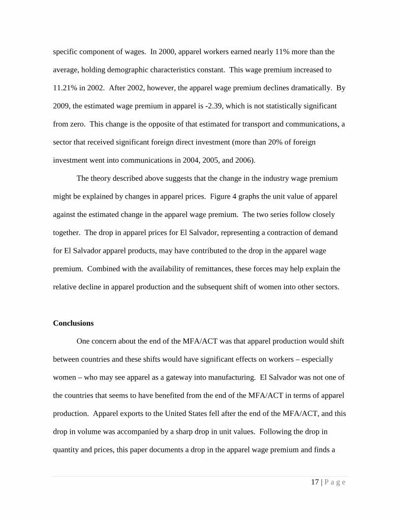
Figure 2 shows the change in prices (unit values) and quantity of U.S. apparel imports
from El Salvador over the 1989-2010 period. Both the price and quantity lines show the rise
and fall U.S. apparel imports from El Salvador. Unit values rise until 1995, level off until the
early 2000s, and drop sharply until 2005. The graph suggests that unit values recover
somewhat between 2005 and 2010.
The change in quantity follows a similar pattern, rising until the early 2000s and then
falling. Together these movements imply several different phases of apparel production.
Rising price and quantity suggests that the first period was characterized by rising demand
7 Log of apparel wages (or manufacturing wages) contained in the ILO’s LABORSTA database. Using log GDP per capita generates similar results. 8 Log of total U.S. apparel exports in 2008 minus log of total apparel exports in 2004, generated from data contained in the OTEXA database. COMTRADE data generates similar results, but not for El Salvador because the El Salvador data entries for HS 61,62, and 63 seem inaccurate.

7 | P a g e
(1989-2000). The second period, 2000-2005, might best be described as falling demand,
since prices and quantities are both falling. The final period, since 2005, might reveal falling
supply, since the quantity falls but prices rise. These periods happen to coincide with
significant events. The first period captures the period immediately following liberalization
and suggests that production was shifting towards apparel. The second period coincides with
China’s entrance into the World Trade Organization (WTO) and a significant surge in
Chinese apparel exports to the world. The last period coincides with the end of the
MFA/ACT, in which factors of production shift out of apparel. A very simple trade model
suggests that wages in particular would be affected by the changes in unit values, so we
briefly sketch out that theory in the next section.
Theory
El Salvador’s globalization experience during the 1995-2011 period is largely
characterized the growth of assembly-based apparel exports. Therefore, it makes sense to
begin with a very simple and canonical trade model and focus on the effects of trade
liberalization on labor’s wages that emerge from that model. The model follows Do et al.
(2011) that adapts Mussa (1974) to “engender trade.” The two main differences from Do et
al. (2011) are that this application is greatly simplified and it uses the model to decompose
the different wage effects of trade liberalization.
Assumes there are two factors, males (m) and females (f), and two industries, apparel
(a) and other activities (b). Output of the two goods (y) can be summarized with linear
homogeneous, differentiable, and positive and declining marginal product production
functions:

8 | P a g e
( , )( , )
a a a
b b b
y X m fy Z m f==
. (1)
We assume full employment of both males and females and that males are fully mobile
between industries.
a bM m m= + (2)
We assume that females are relatively specific. The main reason for this assumption is to
capture the fact that women in developing countries often face strong social pressure to enter
particular industries (such as apparel) and avoid others (perhaps heavy industry). Males,
however, seem more likely to be able to move freely between industries.
Mussa (1974) shows that a change in output prices will have two effects on the
returns to each factor: a short-run effect and a long-run effect. Interpreting women as the
specific factor, the short-run implications for women’s wages are straightforward:
f m
a a a af m
b b b
w p y w mw y w m
= −
= − (3)
This representation assumes that good b is numeriarre and that women are paid the difference
between the value of output and the payment to men. The main implication of (3) is that the
wages of women in the short run are directly related to the price shock in a given industry. In
particular, a change in price to apparel will directly affect women’s wages in apparel and will
not affect women’s wages in industry b.
As Mussa (1974) demonstrates, the effect of a price shock to men, the mobile factor,
is a function of the relative factor intensity of each sector and the degree of factor
substitutability in each industry. In general, however, the per-worker wage rate rises, but not
as much, as the apparel price increases.

9 | P a g e
In the long run, both males and female are mobile between industries and this
problem reduces to the familiar Stolper-Samuelson theorem, in which the effect of the
change on the returns to each factor depends on the relative factor intensities. Defining ijθ as
the share of factor i in industry j this very well-known result is expressed as
ˆ ˆfbfa
ma mb
w pθ
θ θ=
− (4)
and
ˆ ˆm mba
ma mb
w pθθ θ−
=−
. (5)
In words, if apparel is female-intensive and the price of apparel increases, the long run effect
is a real increase in the relative wage of women (in every industry).
The results in equations (3) and (5) can be straightforwardly applied to empirical
estimation through the traditional Mincerian wage equation. This equation is the most
fundamental tool used in wage studies to decompose (or explain) an individual k’s wages as a
function of observable characteristics. While there are slight variations across studies, the
basic form of the Mincerian wage equation is
21 2 3 4ln k k k k k j jk kj
wage female age age education industryα β β β β δ ε= + + + + + +∑ (6)
in which the subscript k indicates the individual, lnwage is the log of earnings and the other
variables are self-explanatory observable demographic characteristics.
This equation can be applied to our model with repeated cross-section data, which
would add a time subscript to each term in equation (6). In our case, the effect of an
increase in industry j’s price would have two effects. In the short run, the increase in price
would affect the industry-specific component of the wage and would show up as a

10 | P a g e
contemporaneous increase in the estimated industry-specific coefficient jδ as implied by
equation (3). The estimated coefficients on the industry dummy variables are interpreted as
“inter-industry wage differentials” following Krueger and Summers (1988).
In the long run, the price increase would affect the “general” component of the wage.
In our application, as long as industry j is female-intensive, an increase in the price of
industry j will affect 1β , which is the economy-wide returns to being female.
One problem with applying this approach is that knowing when the long-run is.
Robertson (2004) provides one of the very few estimates of when the relevant timeframe is
for the “long-run” and suggests that Stolper-Samuelson effects begin to emerge in three to
five years. The next section describes the data used to implement this model.
The key exogenous variable in this model is the output price. The output price can be
considered to be a function of two components. The first is the international price. The
second is the demand for the output given the international price. When the demand goes up
at a given international price, this is the equivalent of having the demand-adjusted price
increase.
Working conditions can fit into this model. The most straightforward way is to
redefine the variable w as compensation that includes working conditions. Working
conditions can be either substitutes or complements for wages. A compensating differential
approach would suggest that wages and working conditions are substitutes: firms with poor
working conditions need to pay workers higher wages to compensate them for enduring the
poor conditions (and pay them less for better conditions).
This approach is appealing theoretically but empirical support is quite mixed. An
alternative perspective is that wages and working conditions are complements. That is, firms

11 | P a g e
with good working conditions may also have higher wages for several reasons. First,
working conditions might be correlated with productivity: better working conditions may
increase worker productivity and possibly wages. Second, improvements in working
conditions may be a form of rent sharing so that more profitable firms might have more
money available to invest in both wages and working conditions. Third, better working
conditions might create a queue of workers that allows firms to select the most productive at
a given wage.
Analyzing plant-level data from Cambodia’s BFC program, Warren and Robertson
(2010) show that wage compliance (that is, compliance with wage laws) is positively
correlated with working conditions. This result suggests that working conditions and wages
are more likely to be complements than substitutes in Cambodian apparel firms – as long as
wage compliance is a good proxy for wages (a measure that is not available in the plant-level
data). In any case, the analysis that follows analyzes changes in the unit values and changes
in wages and working conditions.
Data
El Salvador has a history of collecting labor market and expenditure data through
household surveys. El Salvador conducts the Encuesta de Hogares de Propósitos Múltiples
approximately annually. The survey covers basic demographic information as well as labor
market experience, housing, and other indicators. While data are roughly available from 1989
until the present, survey and sample changes restrict the sample used here to 1995-2010. This
period covers the process of trade liberalization, rising globalization, and the period
following the end of the MFA(ACT).

12 | P a g e
To analyze the surveys together, the analysis focuses on workers with positive wage
earnings (earnings from paid labor). The sample was further restricted to several key
variables: age, gender, education, occupation, sector of employment, geographic area and
remittances.
Table 2 contains sample characteristics. These simple statistics reveal several
important features of the survey data. The first column contains the sample size. These
numbers represent the number of workers in the sample who are between 15 and 65 years old
(inclusive) and have positive earnings from wages. The sample size increases over time.
The mean sample age increases from about 33 years to about 35 years over the 12-year
period covered by the surveys. The female share of the sample increases as well, rising from
about 36.3 percent to 38.0 percent in 2009. The mean education level also increases over
time from 7.68 years to 8.70 years.
Analysis Stylized Facts
Sauré and Zoabi (2009) find trade-related effects on women’s labor force
participation(LFP) in the United States and argue that participation is a critical dimension of
the effects of globalization on labor markets. It is no surprise that in El Salvador, women's
participation in the labor force are lower than women in the United States and that their labor
force participation rates are much smaller than men. Table 3 contains some summary
statistics describing women’s labor force participation calculated by the authors from
household surveys. In El Salvador, labor force participation rates are about 39% for women
and 68% for men. The values for men have changed very little over time, but the overall
labor force participation rate for females has increased from 35.3% in 1997 to 40.8% in 2009.
13 | P a g e
Rising female LFP is a global phenomenon, and is also consistent with Do et al. (2011) who
find a link between female LFP and globalization.
In El Salvador, remittances play a significant role in labor market outcomes because
migration is significant. Participation in the labor force is smaller for those individuals living
in households that receive remittances, about 43% for the former and 55.6% for the latter.
Labor force participation is smaller regardless of sex if you live in a household receiving
remittances. For women the difference in labor force participation between those receiving
remittances and those that does not receive is about 10% to 12.3%. For men the difference is
about 11% to 13.1%. In both cases there is a positive trend in this difference.
The differences for females between remittances and no remittances over time are
especially interesting for this study. Over time the difference between males with
remittances and males without remittances remains relatively constant. For women,
however, the LFP increases for women no receiving remittances, but remains relatively
constant (and, in fact, is lower in 2009 than in 1997) for women receiving remittances.
These figures contribute to the hypothesis that the reservation wage is higher for those
receiving remittances. Remittances may also help explain the shift out of apparel. Rising
reservation wages may make it more difficult to attract workers into apparel and make
production more difficult on the margin.
Table 4 shows the evolution of employment across industries between 2000 and
2009.9
9 Our analysis actually spans 1998-2009, but we present 2000-2009 to save space.
Apparel is one of the larger sectors of the economy. The share of workers in apparel
rises between 2000 and 2003, but starts falling in 2004 until it reaches 5.0% in 2009. The
shares of workers in sales and services increase, consistent with the focus of foreign direct

14 | P a g e
investment in the non-traded sector. These shares are consistent with the pattern of apparel
exports as well.
Table 5 shows the distribution of female employment over time. Table 5 shows that
apparel is especially important to women, following sales and domestic service. Table 5
also shows that there is a clear negative trend in the importance of apparel to women, falling
from 15.2% in 2000 to 8.7% by 2009. This may be the result of both the decline of the sector
and the possibility of the sector becoming more male-intensive, as suggested by Soulé and
Zoabi (2009). As the sector declines (or as males move in), women may shift out of apparel
and into sales and domestic service. The female employment shares of both sales and
domestic service increase through the sample period.
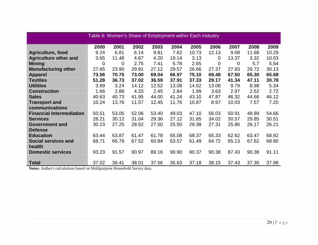
The main reason we focus on women when looking at the effects of the end of the
MFA/ACT is that apparel is female-intensive, both in El Salvador and in most countries.
Table 6 shows the share of workers in each industry that are female. Table 6 shows that the
sectors that females concentrate in (as shown in Table 5) are also very female-intensive.
That is, the female shares of total employment in these industries (apparel, domestic service,
and sales) are much higher than in other industries. About 90% of workers in domestic
service, for example, are female. Interestingly, the share of females in financial
intermediation and education are also quite high – around 50% and 60%, respectively-
throughout the sample.
One of the main messages of Table 6, however, is the falling share of female
employment. This seems consistent with Ozler (2000), who finds that the female share of
employment at the plant level rises with industry-level exports rise in Turkey. Another
possible explanation is that the apparel (and textile) sector experienced significant upgrading

15 | P a g e
over time. Upgrading in the apparel and textile sectors has been linked with rising capital
intensity and a falling demand for women. Together these forces may have significant
implications for wages, and we explore those formally with the following regression analysis.
Estimation Issues
The first estimation issue relates to sample selection. As is well known, female
wages are often censored and therefore when estimating wage equations that include females
it is important to correct for the possible selection bias. To address this issue, we employ the
two-step Heckman approach in which a selection (probit) equation is estimated in the first
stage and from that equation a selection correction variable (the “inverse of the Mills ratio”)
is generated. This selection correction variable is then included in the second-stage wage
equation to control for possible selection effects.
The second estimation issue relates directly to our estimates of interest – the inter-
industry wage differentials. The estimated coefficients on the industry dummy variables are
sensitive to the omitted industry, so Krueger and Summers (1988) suggest an approach that
normalizes the differentials (and approximated the resulting standard errors) so that the
differential estimates do not depend on the omitted industry. Haisken-DeNew and Schmidt
(1997) describe a method that adjusts the differentials and their standard errors so that they
measure the difference between each industry’s wage and the overall mean, rather than the
omitted industry. These differentials are then adjusted by raising e to the power of the
estimated coefficient and subtracting one to adjust for the constant with the log dependent
variable.

16 | P a g e
Main Results
Tables 7A and 7B contain the main results. Table 7A contains the demographic
variables and other controls, and table 7B contains the industry-specific estimates. Each
year represents a separate estimation, so that the results for each year are divided across the
two tables.
Table 7A shows that many of the estimates of the demographic characteristics are
very similar to standard wage equation results. Age has a significant positive but nonlinear
effect on log earning. The “returns” to education are relatively constant, hovering around
5.5%. Interestingly, the coefficient on education rises between 2000 and 2002 and falls for
the rest of the sample. The dummy for urban regions is consistently large and significant.
“Remittances”, “Public Sector” and “Water” are all additional controls to capture some of the
idiosyncratic dimensions of the Salvadoran labor market.
The gap between male and female earnings, holding all other observable demographic
characteristics constant, is about 14% on average across all years. The changes over time,
along with the 95% confidence interval, are shown in figure 3. There is a slight positive
trend in the female dummy coefficient, suggesting a modest closing of the overall wage gap
between demographic-adjusted male and female wages. The size of the confidence interval
relative to the change in the coefficient over time raises the possibility that the change over
time may not be statistically significant. This increase may be modest especially relative to
other countries over this time period, in which the gains to women in other countries have
been large.
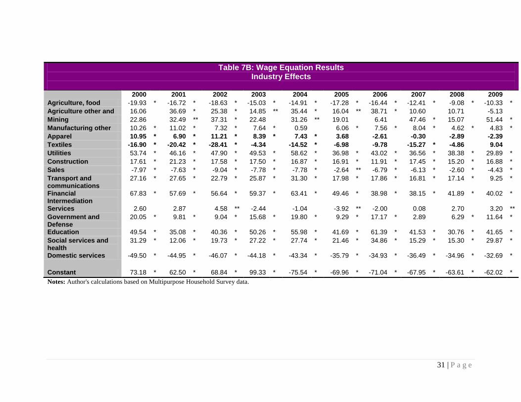
One possible reason for the relatively modest fall in the male-female wage gap may
be the decline of economic opportunities in the apparel sector. Table 7B shows the industry-
17 | P a g e
specific component of wages. In 2000, apparel workers earned nearly 11% more than the
average, holding demographic characteristics constant. This wage premium increased to
11.21% in 2002. After 2002, however, the apparel wage premium declines dramatically. By
2009, the estimated wage premium in apparel is -2.39, which is not statistically significant
from zero. This change is the opposite of that estimated for transport and communications, a
sector that received significant foreign direct investment (more than 20% of foreign
investment went into communications in 2004, 2005, and 2006).
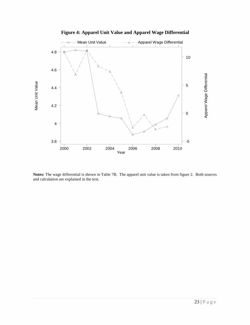
The theory described above suggests that the change in the industry wage premium
might be explained by changes in apparel prices. Figure 4 graphs the unit value of apparel
against the estimated change in the apparel wage premium. The two series follow closely
together. The drop in apparel prices for El Salvador, representing a contraction of demand
for El Salvador apparel products, may have contributed to the drop in the apparel wage
premium. Combined with the availability of remittances, these forces may help explain the
relative decline in apparel production and the subsequent shift of women into other sectors.
Conclusions
One concern about the end of the MFA/ACT was that apparel production would shift
between countries and these shifts would have significant effects on workers – especially
women – who may see apparel as a gateway into manufacturing. El Salvador was not one of
the countries that seems to have benefited from the end of the MFA/ACT in terms of apparel
production. Apparel exports to the United States fell after the end of the MFA/ACT, and this
drop in volume was accompanied by a sharp drop in unit values. Following the drop in
quantity and prices, this paper documents a drop in the apparel wage premium and finds a

18 | P a g e
very small decline in the wage gap between males and females. Compared to other countries,
this modest decline in the male-female wage gap may be at least partially explained by the
loss of otherwise high-paying apparel jobs that were available to women.
This research is limited in several ways, and we hope to address these shortcomings
in later drafts. El Salvador may have had some success in upgrading apparel (and textile)
production. The change in the textile wage premium offers some suggestion of upgrading.
This paper also could be expanded to examine changes in working conditions. Robertson
and Trigueros-Argüello (2009) find that, within manufacturing, working conditions in
apparel are relative high and are particularly “better” than in agriculture. Anecdotal evidence
also has suggested that working conditions in apparel may be preferred to domestic service.
As a result, expanding this study to incorporate working conditions seems like a potentially
fruitful area for future research.

19 | P a g e
References Aguayo-Tellez, Ernesto; Airola, Jim; Juhn,Chinhui (2010)“Did Trade Liberalization Help
Women? The Case of Mexico in the 1990s” NBER Working Paper 16195. Brambilla, Irene; Khandelwal,Amit; Schott, Peter (2007) “Experience Under the Multifiber
Arrangement (MFA) and the Agreement on Textiles and Clothing (ATC)” NBER Working Paper 13346.
Do, Quy-Toan; Levchenko,Andrei A.; Raddatz, Claudio (2011) “Engendering Trade” background paper for the World Development Report 2012 on Gender Equality and Development, World Bank.
Haisken-DeNew, J.P. and Schmidt, C. (1997) “Inter-industry and Inter-region Differentials: Mechanics and Interpretation” The Review of Economics and Statistics 79(3): 516-521.
Heckman, James J. (1979) “Sample Selection Bias as a Specification Error” Econometrica 47: 153-161.
Krueger, A. B. and Summers, L.H. (1987) “Reflections on the Inter-Industry Wage Structure” in Lang, K. and Leonard, S (eds.) Unemployment and the Structure of Labor Markets Basil Blackwell:17-47.
Mussa, Michael (1974) “Tariffs and the Distribution of Income: The Importance of Factor Specificity, Substitutability, and Intensity in the Short and Long Run” The Journal of Political Economy, Nov. - Dec., 82( 6): 1191-1203.
Oostendorp, Remco H. (2009)“Globalization and the Gender Wage Gap” World Bank Economic Review, Oxford University Press, January, 23(1):141-161.
Özler, Şule (2000) “Export Orientation and Female Share of Employment: Evidence from Turkey” World Development 28(7): 1239-1248.
Özler, Şule (2001) “Export Led Industrialization and Gender Differences in Job Creation and Destruction: Micro Evidence from the Turkish Manufacturing Sector” Economic Research Forum, Cairo, Working Paper 116.
Qian, Michelle (2008) “Missing Women and the Price of Tea in China: The Effect of Sex-Specific Earnings on Sex Imbalance” Quarterly Journal of Economics July 123(3): 1251-1285.
Rendall, Michelle (2010) “Brain Versus Brawn” The Realization of Women’s Comparative Advantage” SSRN eLibrary.
Rivera Campos, Roberto (2000) “La economía salvadoreña al final del siglo: Desafíos para el futuro”, FLACSO-El Salvador.
Robertson, Raymond and Alvaro Trigueros-Argüello (2009) “The Effects of Globalization on Working Conditions:El Salvador 1995-2005” in Robertson, Raymond; Brown, Drusilla; Pierre, Gaëlle; Sanchez-Puerta, Laura (eds.) (2009) Globalization,Wages, and the Quality of Jobs Five Country Studies, The World Bank, Washington, D.C.
Sauré, Philip and HosnyZoabi (2009) “Effects of Trade on Female Labor Force Participation” Swiss National Bank Working Papers 2009-12.
Warren, Cael, and Raymond Robertson "Globalization and the Wage-Working Conditions Relationship: A Case Study of Cambodian Garment Factories", mimeo, Macalester College. May 2010.

20 | P a g e
Figure 1: Log Change in U.S. Imports as a Function of Apparel Wage
Notes: The apparel wage is the log of the hourly wage in apparel (or manufacturing) for each country as found in the LABORSTA database of the ILO (http://laborsta.ilo.org/). The U.S. import data are for all apparel categories and are from the OTEXA database (http://otexa.ita.doc.gov/). The change in imports is the difference in the log of total imports in 2008 minus the log of total imports in 2004. The horizontal line denotes zero and the slope (standard error) of the fitted line is -0.476 (0.064) with an adjusted R-square value of 0.453. The only other variable included in the regression was the square of the log wage, which was statistically insignificant. The regression and graph use 2004 U.S. import values as weights.
Log Wage MFA
Fitted values Change in US Imports 2004-2008
-2 0 2 4
-1.5
-1
-.5
0
.5
1
1.5
India
CambodiaEgypt
M auri ti u
Sri Lank
Pakistan
Bulgar ia
China
El Salva
B ot sw an a
Indonesi
Philippi
A lba nia
Romania
U krai ne
Nicaragu
Jordan
Thailand
Peru
E cu ad or
Korea, R
T an za nia
L at via
B oli via
L ith ua ni
Guatemal
MexicoG u ya na
P ar ag ua y
C ze ch R e
H ungary
A rg en tin
P oland
Brazil
C ro at ia
Macau, C
Malaysia
P an am a
Portugal
Swazilan
G r ee ce
S lov en ia
Hong Kon
S pain
F re nc h G
C yp ru s
France
Taiwan, Israel
Turkey
Canada
N et he rla
A us tr ia
S ingapor
I re lan d
B elg ium
S we de n
United K
S wi tzer l
I ce lan d
N or wa y
N et he rla
D en m ar k
B er m ud a
El Salvador
21 | P a g e
Figure 2: U.S. Apparel Imports from El Salvador:
Unit Value and Total Quantity
Notes: Authors’ elaboration using data from OTEXA (http://otexa.ita.doc.gov/). SME stands for “Square Meter Equivalent”, the common units used to measure various types of apparel. Unit value is calculated by dividing total (nominal) value of each product by the quantity imported of that product. The value here is the simple (unweighted) average across all products and months within a given year for U.S. imports from El Salvador. The quantity is the sum across all products and months within each year for U.S. imports from El Salvador.
Mea
n U
nit V
alue
Year
Tota
l Qua
ntity
(SM
E)
Mean Unit Value Total Quantity (SME)
1990 1995 2000 2005 2010
3.2
3.6
4
4.4
4.8
0
500
1000

22 | P a g e
Figure 3: The Change in the Female Wage Gap over Time (95% Confidence Interval)
-.18
-.16
-.14
-.12
-.1
1998 2000 2002 2004 2006 2008year
23 | P a g e
Figure 4: Apparel Unit Value and Apparel Wage Differential
Notes: The wage differential is shown in Table 7B. The apparel unit value is taken from figure 2. Both sources and calculation are explained in the text.
Mea
n U
nit V
alue
Year
App
arel
Wag
e D
iffer
entia
l
Mean Unit Value Apparel Wage Differential
2000 2002 2004 2006 2008 2010
3.8
4
4.2
4.4
4.6
4.8
-5
0
5
10

24 | P a g e
Table 1: El Salvador: Foreign Direct Investment (position data)
US$ Millions
2000 2001 2002 2003 2004 2005 2006 2007 2008 2009/III INVERSION EXTRANJERA TOTAL 1,973.0 2,252.1 3,133.6 3,275.5 3,655.4 4,166.4 4,407.8 5,916.2 6,701.2 6,878.7 Equity Capital and Reinvested Earnings
1,973.0 2,252.1 2,459.9 2,589.3 2,996.0 3,508.0 3,735.1 5,182.5 5,721.4 5,891.1
1 Industry 336.5 401.1 447.8 496.1 536.9 853.5 870.2 891.6 919.7 936.6 2 Sales 169.1 190.2 225.9 239.2 278.3 305.0 356.3 397.3 411.9 430.8 3 Services 70.0 90.0 109.4 110.9 110.8 125.2 137.1 177.2 184.2 192.5 4 Construction 12.2 12.3 12.3 12.4 12.4 12.4 12.4 12.3 12.3 12.3 5 Communications 291.0 352.6 401.2 411.3 746.0 793.8 793.9 860.6 917.4 927.9 6 Electricity 806.9 821.5 848.2 848.2 800.2 800.2 847.6 847.6 879.5 879.5 7 Agriculture and Fishing 10.0 40.0 48.5 46.8 68.6 67.1 67.7 69.6 69.6 69.6 8 Mines and "Canteras" 0.0 0.0 0.0 0.0 0.0 1.5 29.5 37.8 42.5 43.3 9 Financial 120.4 161.8 173.9 161.1 148.1 250.4 321.9 1,489.4 1,858.9 1,902.5 10 Maquila 156.9 182.6 192.7 263.3 294.7 298.9 298.5 399.1 425.4 496.1 1,973.1 2,252.1 2,460.0 2,589.2 2,996.1 3,508.1 3,735.0 5,182.5 5,721.5 5,891.1 Change over previous year (FLOWS)
279.0 207.9 129.2 406.9 512.0 226.9 1,447.5 539.0 169.6
Intercompany Transactions 0.0 0.0 673.7 686.2 659.4 658.4 672.7 733.7 979.8 987.6 Flujos 262.3 12.6 -26.8 93.3 1,973.1 2,252.1 3,133.7 3,275.4 3,655.5 4,166.5 4,407.7 5,916.2 6,701.3 6,878.7 Tradable/Non-tradable grouping Tradable Sector 503.4 623.7 689.0 806.2 900.2 1,221.0 1,265.9 1,398.1 1,457.2 1,545.6 Non Tradable Sector 1,469.6 1,628.4 1,770.9 1,783.1 2,095.8 2,287.0 2,469.2 3,784.4 4,264.2 4,345.5 Shares (%) Tradable Sector 25.5 27.7 28.0 31.1 30.0 34.8 33.9 27.0 25.5 26.2 Non Tradable Sector 74.5 72.3 72.0 68.9 70.0 65.2 66.1 73.0 74.5 73.8 Notes: Elaborated by the authors using data from the Banco Central de Reserva de El Salvador.

25 | P a g e
Table 2: Sample Characteristics for Employed Workers Year Sample
size Mean age
(years) Female Share
Mean education
(years) 1998 10,877 33.22 36.3 7.68 1999 14,861 33.45 36.9 7.85 2000 13,833 33.70 37.0 7.71 2001 10,443 33.86 36.4 8.21 2002 13,531 34.07 38.0 8.58 2003 14,451 33.43 37.6 8.38 2004 14,290 33.90 35.6 8.31 2005 13,894 34.33 37.2 8.54 2006 14,119 34.28 38.2 8.52 2007 14,708 34.78 37.4 8.69 2008 14,580 34.64 37.3 8.66 2009 16,644 34.93 38.0 8.70
Notes: Authors’ calculations based on Multipurpose Household Survey data. The definition of Working Population is age>15 years old = 16 years or older. The definition of employed workers includes only full and part time wage workers, and with a positive wage rate (no missing values).

26 | P a g e
Table 3: Labor Force Participation
(Percent)
Total
Remittances
Women
Men
Year MEN WOMEN ALL NO REMI REMITT NO REMI REMITT NO REMI REMITT 1997 68.5 35.3 50.9 1998 69.6 39.3 53.5 55.3 45.9 40.7 33.9 71.4 61.6 1999 68.1 39.1 52.6 54.9 43.6 40.9 32.5 70.4 58.2 2000 67.7 38.7 52.2 54.6 42.9 40.9 30.8 69.7 58.7 2001 69.2 39.5 53.3 55.7 44.4 41.6 32.0 71.4 60.5 2002 65.8 38.6 51.2 54.0 41.4 41.1 30.5 68.5 55.7 2003 68.3 40.4 53.4 56.3 42.9 43.2 31.4 70.6 58.6 2004 66.5 38.6 51.7 54.6 41.7 41.3 30.0 68.9 57.2 2005 67.4 39.5 52.4 55.9 41.9 42.8 30.5 70.4 57.3 2006 67.0 40.4 52.6 56.4 41.1 44.1 29.8 70.0 56.5 2007 68.0 40.0 52.9 56.2 44.0 43.3 32.2 70.6 60.2 2008 68.7 40.4 53.5 56.7 43.9 43.6 31.7 71.2 60.1 2009 68.7 40.8 53.7 56.5 44.0 43.5 32.0 70.9 60.1
Notes: Authors’ calculations based on household surveys as described in the text.

27 | P a g e
Table 4: Industry Employment Shares
All Workers
Industry 2000 2001 2002 2003 2004 2005 2006 2007 2008 2009 Agriculture, food 14.3 13.5 11.4 11.9 14.9 14.2 14.4 11.8 13.2 14.8 Agriculture other and 0.3 0.4 0.3 0.4 0.3 0.2 0.2 0.4 0.3 0.7 Mining 0.1 0.2 0.2 0.1 0.1 0.1 0.1 0.2 0.2 0.1 Manufacturing other 12.4 12.0 12.5 11.2 10.9 11.0 10.5 10.9 12.2 11.3 Apparel 7.6 7.0 7.6 8.6 7.3 5.9 5.9 5.9 6.0 5.0 Textiles 1.0 1.0 1.0 0.6 0.6 0.7 0.7 0.9 1.1 0.4 Utilities 0.6 0.8 0.8 0.4 0.7 0.5 0.7 0.7 0.9 0.5 Construction 7.3 8.1 8.6 9.3 8.9 8.4 9.3 8.6 8.1 7.1 Sales 16.0 16.0 16.8 17.5 18.0 17.8 18.8 19.4 19.3 19.7 Transport and communications
5.9 6.1 5.4 5.4 6.1 5.9 5.5 5.6 5.0 4.9
Financial Intermediation 2.1 2.4 2.2 1.8 1.3 1.9 1.7 2.1 2.1 1.9 Services 5.7 6.5 6.6 7.0 6.4 7.7 7.0 7.5 6.9 7.7 Government and Defense 9.6 7.2 7.7 7.2 6.6 7.0 6.7 7.1 7.2 7.4 Education 5.3 6.4 7.1 5.8 5.8 6.8 5.9 6.4 5.5 5.8 Social services and health 4.4 4.5 4.3 4.8 4.2 4.2 4.4 4.7 4.4 4.4 Domestic services 7.5 8.1 7.5 7.8 7.8 7.6 8.3 7.8 7.9 8.3 Total 100.0 100.0 100.0 100.0 100.0 100.0 100.0 100.0 100.0 100.0 Notes: Author's calculations based on Multipurpose Household Survey data.

28 | P a g e
Table 5: Distribution of Female Employment across Industries
Industry 2000 2001 2002 2003 2004 2005 2006 2007 2008 2009 Agriculture, food 3.6 2.5 1.8 3.1 3.2 4.1 4.6 2.9 4.1 4.0 Agriculture other and 0.0 0.1 0.0 0.1 0.2 0.0 0.0 0.1 0.0 0.2 Mining 0.0 0.0 0.0 0.0 0.0 0.0 0.0 0.0 0.0 0.0 Manufacturing other 9.3 7.9 9.9 8.1 9.0 7.9 7.5 8.1 9.7 9.0 Apparel 15.2 13.5 14.6 15.9 13.8 12.0 10.7 10.6 10.4 8.7 Textiles 1.3 1.0 1.0 0.6 0.6 0.7 0.5 1.0 1.3 0.4 Utilities 0.1 0.1 0.3 0.2 0.3 0.2 0.2 0.2 0.2 0.1 Construction 0.3 0.6 1.0 0.6 0.7 0.5 0.9 0.7 0.6 0.5 Sales 17.6 17.9 18.5 20.5 20.9 20.7 23.6 24.0 23.0 23.9 Transport and communications
1.6 2.3 1.7 1.8 2.0 1.7 1.3 1.5 1.0 0.9
Financial Intermediation 2.8 3.4 3.0 2.6 1.8 2.4 2.4 2.9 2.8 2.8 Services 4.4 5.4 5.4 5.5 4.9 6.5 6.3 6.1 5.5 6.2 Government and Defense 7.9 5.4 5.8 5.3 4.8 5.6 4.8 4.9 5.0 5.1 Education 9.1 11.2 11.5 9.6 10.7 12.4 10.0 10.7 9.3 10.4 Social services and health 8.2 8.2 7.7 7.8 7.5 7.0 7.4 8.1 8.0 7.9 Domestic services 18.8 20.4 17.9 18.6 19.8 18.3 19.7 18.2 19.1 20.0 Total 100.0 100.0 100.0 100.0 100.0 100.0 100.0 100.0 100.0 100.0 Notes: Author's calculations based on Multipurpose Household Survey data.
29 | P a g e
Table 6: Women’s Share of Employment within Each Industry
2000 2001 2002 2003 2004 2005 2006 2007 2008 2009 Agriculture, food 9.24 6.81 6.14 9.81 7.62 10.73 12.13 9.08 11.68 10.29 Agriculture other and 3.65 11.48 4.67 4.20 19.14 3.13 0 13.37 3.32 10.03 Mining 0 0 2.75 7.41 5.78 2.65 0 0 5.7 5.54 Manufacturing other 27.65 23.90 29.91 27.12 29.57 26.66 27.37 27.83 29.72 30.13 Apparel 73.56 70.75 73.00 69.04 66.97 75.10 69.48 67.50 65.30 65.68 Textiles 51.28 36.73 37.02 36.59 37.91 37.33 29.17 41.34 47.11 30.78 Utilities 3.99 3.24 14.12 12.52 13.08 14.52 13.08 9.79 8.98 5.34 Construction 1.66 2.88 4.33 2.45 2.84 1.99 3.63 2.97 2.52 2.72 Sales 40.63 40.73 41.95 44.00 41.24 43.10 47.87 46.32 44.66 46.12 Transport and communications
10.24 13.76 11.57 12.45 11.76 10.87 8.97 10.03 7.57 7.20
Financial Intermediation 50.51 53.05 52.06 53.40 49.03 47.10 56.03 50.91 48.89 54.66 Services 28.21 30.12 31.04 29.36 27.12 31.65 34.02 30.57 29.85 30.51 Government and Defense
30.23 27.25 28.52 27.50 25.50 29.38 27.31 25.86 26.17 26.21
Education 63.44 63.87 61.47 61.78 65.08 68.37 65.33 62.62 63.47 68.92 Social services and health
68.71 66.79 67.52 60.84 63.57 61.49 64.72 65.13 67.62 68.80
Domestic services 93.23 91.57 90.97 89.16 90.90 90.37 90.38 87.43 90.38 91.11 Total 37.02 36.41 38.01 37.56 35.63 37.18 38.15 37.43 37.35 37.98 Notes: Author's calculations based on Multipurpose Household Survey data.

30 | P a g e
Table 7A: Waqe Equation Results
Demographic Characteristics
2000 2001 2002 2003 2004 2005 2006 2007 2008 2009 Age 4.68 * 4.69 * 4.46 * 3.97 * 3.67 * 3.53 * 4.12 * 3.84 * 3.21 * 3.40 * Age squared -0.05 * -0.05 * -0.04 * -0.04 * -0.03 * -0.03 * -0.04 * -0.04 * -0.03 * -0.03 * Years of Education
5.28 * 6.69 * 6.42 * 5.87 * 5.70 * 5.39 * 5.59 * 5.31 * 5.40 * 4.94 *
Urban dummy 8.97 * 4.62 * 5.96 * 6.45 * 8.45 * 5.56 * 8.26 * 5.74 * 5.98 * 4.91 * Female -13.05 * -14.67 * -16.07 * -13.48 * -14.53 * -13.97 * -12.43 * -12.66 * -11.71 * -13.49 * Public sector dummy
47.86 * 47.43 * 42.13 * 41.01 * 35.14 * 37.76 * 30.62 * 54.41 * 50.51 * 47.95 *
Remittances 0.14 -0.62 1.95 -1.66 2.33 4.53 * 2.77 ** 2.22 0.60 1.61 Water dummy 8.72 * 6.49 * 5.48 * 2.69 ** 0.36 5.00 * -0.91 0.43 -6.61 * -4.52 * Notes: Author's calculations based on Multipurpose Household Survey data. Each year was estimated separately. The results for each year are split between tables 7A (demographic characteristics) and 7B (industry effects).
31 | P a g e
Table 7B: Wage Equation Results
Industry Effects
2000 2001 2002 2003 2004 2005 2006 2007 2008 2009 Agriculture, food -19.93 * -16.72 * -18.63 * -15.03 * -14.91 * -17.28 * -16.44 * -12.41 * -9.08 * -10.33 * Agriculture other and 16.06 36.69 * 25.38 * 14.85 ** 35.44 * 16.04 ** 38.71 * 10.60 10.71 -5.13 Mining 22.86 32.49 ** 37.31 * 22.48 31.26 ** 19.01 6.41 47.46 * 15.07 51.44 * Manufacturing other 10.26 * 11.02 * 7.32 * 7.64 * 0.59 6.06 * 7.56 * 8.04 * 4.62 * 4.83 * Apparel 10.95 * 6.90 * 11.21 * 8.39 * 7.43 * 3.68 -2.61 -0.30 -2.89 -2.39 Textiles -16.90 * -20.42 * -28.41 * -4.34 -14.52 * -6.98 -9.78 -15.27 * -4.86 9.04 Utilities 53.74 * 46.16 * 47.90 * 49.53 * 58.62 * 36.98 * 43.02 * 36.56 * 38.38 * 29.89 * Construction 17.61 * 21.23 * 17.58 * 17.50 * 16.87 * 16.91 * 11.91 * 17.45 * 15.20 * 16.88 * Sales -7.97 * -7.63 * -9.04 * -7.78 * -7.78 * -2.64 ** -6.79 * -6.13 * -2.60 * -4.43 * Transport and communications
27.16 * 27.65 * 22.79 * 25.87 * 31.30 * 17.98 * 17.86 * 16.81 * 17.14 * 9.25 *
Financial Intermediation
67.83 * 57.69 * 56.64 * 59.37 * 63.41 * 49.46 * 38.98 * 38.15 * 41.89 * 40.02 *
Services 2.60 2.87 4.58 ** -2.44 -1.04 -3.92 ** -2.00 0.08 2.70 3.20 ** Government and Defense
20.05 * 9.81 * 9.04 * 15.68 * 19.80 * 9.29 * 17.17 * 2.89 6.29 * 11.64 *
Education 49.54 * 35.08 * 40.36 * 50.26 * 55.98 * 41.69 * 61.39 * 41.53 * 30.76 * 41.65 * Social services and health
31.29 * 12.06 * 19.73 * 27.22 * 27.74 * 21.46 * 34.86 * 15.29 * 15.30 * 29.87 *
Domestic services -49.50 * -44.95 * -46.07 * -44.18 * -43.34 * -35.79 * -34.93 * -36.49 * -34.96 * -32.69 * Constant 73.18 * 62.50 * 68.84 * 99.33 * -75.54 * -69.96 * -71.04 * -67.95 * -63.61 * -62.02 * Notes: Author's calculations based on Multipurpose Household Survey data.


![Enfraquecimento Do Legislativo Ligia[1]](https://static.fdocuments.in/doc/165x107/55cf8f80550346703b9d0376/enfraquecimento-do-legislativo-ligia1.jpg)