
Analysis of dissipation and di usion mechanisms modeled by ...
76
Analysis of dissipation and diffusion mechanisms modeled by nonlinear PDEs in developmental biology and quantum mechanics. M. del Pilar Guerrero Contreras, Departamento Matem´ atica Aplicada, Granada. July 21, 2010
Transcript of Analysis of dissipation and di usion mechanisms modeled by ...
Analysis of dissipation and diffusion mechanismsmodeled by nonlinear PDEs in developmental
biology and quantum mechanics.
M. del Pilar Guerrero Contreras,Departamento Matematica Aplicada,
Granada.
July 21, 2010

Editor: Editorial de la Universidad de GranadaAutor: María del Pilar Guerrero ContrerasD.L.: GR 4260-2010ISBN: 978-84-693-5974-7

palabra

i
La presente memoria, titulada ”Analysis of dissipation and diffusion mecha-nisms modeled by nonlinear PDEs in developmental biology and quantum me-chanics”, ha sido realizada bajo la direccion de los doctores Juan S. Soler Vizcaınoy Jose Luis Lopez Fernandez del Departamento de Matematica Aplicada de laUniversidad de Granada, para obtener el tıtulo de Doctor en Matematicas por laUniversidad de Granada.
V.B. Director V.B. Director
Fdo: Juan S. Soler Vizcaıno Fdo: Jose Luis Lopez Fernandez
La doctoranda
Fdo: M. Pilar Guerrero Contreras

palabra

iii
Para Tales... la cuestion no era que sabemos,sino como lo sabemos.
Aristoteles

palabra

v
AGRADECIMIENTOS
Cuando hace mas de cuatro anos empece esta tesis doctoral no podıa imaginarni por asomo como iba a crecer mi mundo interior. Lo que parecıa un reto personalse convirtio desde el primer momento en un extraordinario ejercicio de inteligenciacolectiva, en un ir y venir de retos que solo he podido superar con la ayuda demi gente. A todos ellos les debo una parte de esta memoria y no puedo mas queagradecerles que hayan querido compartir esta aventura conmigo.
De corazon, muchas gracias:A Juan Soler y Jose Luis por su dedicacion durante estos anos y por plantearme
nuevas lıneas de trabajo que forman parte de esta tesis.A los miembros del tribunal por haber querido ser testigos de mi trabajo.Al Departamento de Matematica Aplicada por poner a mi disposicion un
espacio que hoy siento como mıo.A Juanjo, Oscar y Juan Campos por todo lo que he aprendido a su lado.A Jesus por sus reflexiones de de-coherencia.A mis companeros de despacho y al resto de miembros del grupo de investi-
gacion, por hacerme reır y ayudarme a madurar en la Ciencia.A los que me rodearon en los desayunos, por anadir Algebra y Geometrıa a
mi cafe con leche.A quienes me acompanaron en las noches de vinos y conversacion por amenizar
los recodos del camino.A todos los que me ayudaron a ver el mundo con los ojos de la curiosidad,
tan necesaria para la investigacion.A los profesores que me guiaron durante la licenciatura.A Manuel Ortiz por despertar mi interes por las matematicas en mi ninez.A Marıa Jose por ensenarme a ver las cosas desde otro punto de vista.A Macarena por contagiarme ilusion todos los dıas, leerse y valorar esta tesis
como suya.A mis amigos porque todos creyeron en mı y me apoyaron.A Jaume, por entender mis ausencias mentales, en especial los ultimos meses.Y consciente de haber dejado lo mas importante para el final, muchas gracias a
mi familia: a mi padre por sentarse conmigo a pensar los problemas matematicos,a mi madre por aguantar mi mal humor, a mis hermanas y a Leyre por hacermesonreır siempre que lo he necesitado.
Cuando emprendas tu viaje a ItacaPide que el camino sea largo,
Lleno de aventuras, lleno de experiencias.Pide que el camino sea largo.
Fragmento del poema ”Itaca” de Constantin P. Kavafis

vi

Contents
1 Introduction 3
2 A wavefunction description of stochastic–mechanical Fokker–Planckdissipation 72.1 Introduction . . . . . . . . . . . . . . . . . . . . . . . . . . . . . . 72.2 The wavefunction approach . . . . . . . . . . . . . . . . . . . . . 92.3 Steady state dynamics . . . . . . . . . . . . . . . . . . . . . . . . 13
2.3.1 Vanishing local diffusion current . . . . . . . . . . . . . . . 132.4 Numerical evidence accounting for negative dissipation in the log–
law Schrodinger equation . . . . . . . . . . . . . . . . . . . . . . . 162.4.1 Exact solutions of the quantum Fokker–Planck master equa-
tion . . . . . . . . . . . . . . . . . . . . . . . . . . . . . . 162.4.2 The numerical algorithm . . . . . . . . . . . . . . . . . . . 18
2.5 Summary and conclusions . . . . . . . . . . . . . . . . . . . . . . 21
3 Global H1 solvability of the 3D logarithmic Schrodinger equation 273.1 Introduction and main result . . . . . . . . . . . . . . . . . . . . . 273.2 Global well–posedness of a sequence of approximate problems . . 29
3.2.1 A priori estimates: ε–local existence . . . . . . . . . . . . 303.2.2 Approximation of the logarithmic nonlinearity . . . . . . . 303.2.3 ε–local existence . . . . . . . . . . . . . . . . . . . . . . . 313.2.4 A posteriori estimates: ε–global existence . . . . . . . . . 33
3.3 Passing to the limit ε→ 0: Global solvability in H1(R3) . . . . . 36
4 On the analysis of travelling waves to a nonlinear flux limitedreaction–diffusion equation 394.1 Introduction and main results . . . . . . . . . . . . . . . . . . . . 394.2 An equivalent problem for classical travelling waves . . . . . . . . 44
4.2.1 Travelling wave equations . . . . . . . . . . . . . . . . . . 444.2.2 Proof of Proposition 2.1 . . . . . . . . . . . . . . . . . . . 484.2.3 Existence of roots for (4.15) . . . . . . . . . . . . . . . . . 504.2.4 Proof of Lemma 2.4 . . . . . . . . . . . . . . . . . . . . . . 51
4.3 Entropy solutions and consequences . . . . . . . . . . . . . . . . . 53
vii

viii CONTENTS

Introduccion
Esta tesis se centra en el analisis de algunos aspectos cualitativos relacionadoscon ecuaciones diferenciales parciales que surgen en la biologıa del desarrollo yla mecanica cuantica. La idea de fondo que vinculan los diferentes problemas enestudio es el control de esas propiedades de las soluciones relativas a la difusion,la dispersion o disipacion en contraste con en dichos modelos fısicos considerados.En este espıritu, la Tesis se han abordado y discutido los distintos enfoques delconcepto de difusion en mecanica cuantica y la biologıa, lo que constituye unaspecto crucial en el presente y el futuro del desarrollo de estos campos. Aquı,hemos utilizado diferentes herramientas matematicas para analizar los objetivosanteriores: el modelado, ası como el buen-planteamiento en el marco funcionalde los espacios de Sobolev, propiedades dinamicas de las ondas viajeras, las solu-ciones de entropıa, puntos que en el mismo tiempo contribuyen a enriquecer lavariedad de temas y contenidos de la tesis.
Vamos a describir brevemente los temas concretos y los resultados de estatesis. El capıtulo 2 esta dedicado al modelado de procesos de disipacion/difusioncuantica. El marco teorico habitual para este tipo de estudios es el de los sis-temas cuanticos abiertos, en los que se analiza la interaccion entre el sistemade interes y el ambiente. De esta manera se establece la ecuacion maestra quegobierna la evolucion temporal del operador de densidad (reducido) ρ de nue-stro sistema. Una interpretacion cinetica de ρ permite asociarle una funcion de(pseudo-) probabilidad W , cuya evolucion temporal responde a una ecuacion contermino de transporte. En nuestro caso dicha ecuacion llevara acoplado un nucleode Fokker–Planck para describir efectos de disipacion. La ecuacion de WFP esla siguiente
∂W
∂t+ (ξ · ∇x)W + Θ[V ]W = LQFP [W ] ,
con
LQFP [W ] =Dpp
m2∆ξW + 2λ∇ξ · (ξW ) +
2Dpq
m∇x · (∇ξW ) +Dqq∆xW .
La ecuacion de WFP puede verse como una generalizacion del modelo deCaldeira–Leggett [22] (el mas comunmente aceptado que describe efectos de disi-pacion) que esta en la forma de Lindblad [69].
Aunque la formulacion cinetica presenta ventajas respecto al tratamiento deρ tambien conlleva algunos inconvenientes: en primer lugar la funcion W no
ix
x CONTENTS
puede interpretarse como una funcion de probabilidad con sentido completo yaque puede tomar valores negativos. Por otra parte, la formulacion cinetica estadefinida en el espacio de fase, por lo que que el tratamiento es mas costoso.Ademas los fenomenos cuanticos usualmente se describen en terminos de unafuncion de onda ψ por lo que es interesante representar los efectos de disipaciony difusion en la fomulacion de Schrodinger, admitiendo terminos no lineales.
Nuestro primer objetivo es establecer un modelo de Schrodinger que representela misma fısica que WPF. Para ello interpretaremos la ecuacion de continuidadasociada a WFP como resultado de un proceso de difusion gobernada a nivelmicroscopico por movimiento Browniano, obteniendo la siguiente ecuacion deSchrodinger
iα∂ψ
∂t= − α
2
2m∆xψ + V ψ +
α2
~2Qψ + Λ log(n)ψ +Dqq
(iα
2
∆xn
n+m∇x ·
J
n
)ψ .
La no linealidad de esta ecuacion de Schrodinger, se reduce a un solo potencial,el termino logarıtmico, por medio de una transformacion Gauge. Por ello resultainteresante el estudio de la ecuacion simplificada ya que la fısica de ambos proble-mas es la misma. En el capıtulo 3 se estudia la existencia y unicidad de solucionesen todo el espacio de la ecuacion de Schrodinger puramente logaritmica.
El resultado principal desarrollado en el capıtulo 3 es la prueba de la existenciade una unica solucion global en tiempo en sentido mild en H1(R3), del problemade valores iniciales
i∂ψ
∂t= −D∆ψ + σlog(n)ψ , (t, x) ∈ [0,∞)× R3 , (1)
ψ(0, x) = ψ0(x) , ψ0 ∈ H1(R3) , |x|n0 ∈ L1(R3) , (2)
bajo la unica hipotesis de que el momento de inercia inicial∫
R3 |x|n0 dx sea finito,este estudio es independiente del signo que acompana al logarıtmo, donde seha denotado n0(x) = n(0, x). El principal objetivo consiste en el desarrollo deuna teorıa matematica del buen planteamiento en todo el espacio en H1(R3), sinninguna restriccion del espacio funcional a fin de evitar la singularidad del poten-cial logarıtmico en el origen ni las condiciones tecnicas que permiten garantizara priori la convergencia de la secesion de soluciones aproximadas. El resultadoprincipal es el siguiente teorema
Teorema 1 Existe una unica funcion
ψ ∈ L∞([0,∞);H1(R3)) ∩ C([0,∞);L2(R3))
la cual es solucion del problema de valores iniciales (1.1)–(1.2) en un sentidomild.
En el Capıtulo 4 se ha lleva a cabo una modificacion del efecto de difusionligado a la ley de Fick, ya que no describe la realidad de los modelos biologicos

CONTENTS 1
porque se produce la difusion en todo el espacio de manera instantanea , paraaproximarnos a la realidad de este proceso se ha modificado Fick segun un terminono lineal que aparece por primera vez en [88], tambien aparece en el marco detransporte de masa optimo [19].
Una vez llevada acabo esta modificacion se han estudiado un tipo de solu-ciones especiales de las ecuaciones de RD que tiene un papel importante en lasaplicaciones, para el caso escalar se denominan ondas viajeras y para el casode sistema formacion de patrones. Dadas las caracterısticas que las soluciones deondas viajeras tienen son muy utiles en modelacion en diferentes areas como inva-siones biologicas [24], epidemias [93], crecimiento de tumores [21] . Consideramosel caso escalar de la ecuacion modificada con un termino de reaccion del tipo deFisher Kolmogorov–PP (f(u)) y haremos la clasificacion de ondas viajeras segunla velocidad de avance del soporte de la solucion y la viscosidad.
El principal resultado descrito en el Capıtulo 4 de esta memoria da las condi-ciones para la existencia de soluciones de tipo onda viajera de la ecuacion
∂u
∂t= ν∂x
u∂xu√|u|2 + ν2
c2|∂xu|2
+ f(u), u(t = 0, x) = u0(x), (3)
Teorema 2 En terminos de un valor de σ∗ ≤ c, dependiendo de ν, c, y k, existeun frente de onda que es
(i) una solucion clasica para (4.2), con velocidad de onda σ > σ∗ o σ = σ∗ < c;
(ii) una solucion de entropıa discontinua para (4.2), con velocidad de onda σ =σ∗ = c.
La existencia de soluciones de ondas viajeras en el caso para σ < σ∗ es unproblema abierto. Tambien, la existencia de otra clase de ondas viajeras talescomo pulsos o solitones podrıan estudiarse (vease por ejemplo [87], o [44] en otrocontexto).

2 CONTENTS

Chapter 1
Introduction
This Thesis is focused on the analysis of some qualitative aspects related to partialdifferential equations arising in developmental biology and quantum mechanics.The basic idea linking the different problems under study is the scrutiny of thoseproperties of the solutions concerning diffusion, dispersion or dissipation in con-trast with the physical inputs of the models considered. In this spirit, the Thesisdeals with and discuss the various approaches to the concept of diffusion in quan-tum mechanics and biology, which constitutes a crucial aspect in the present andthe future of the development of both fields. Here, different mathematical toolscome together in order to analyze the above general objectives: modeling, inter-phase fluid flows, well–posedness in the functional framework of Sobolev spaces,dynamic properties of traveling waves, entropy solutions, . . . , that at the sametime contribute to enrich the variety of topics and contents of the Thesis.
Let us briefly describe the specific subjects and results of this Thesis. Thesecond chapter is devoted to the modeling of quantum dissipation processes. Thetheoretical framework supporting this sort of phenomena is that of open quantumsystems, which takes into account the interactions among the particle ensembleunder study and the environment. This is actually the starting point to derivethe master equation governing the temporal evolution of the (reduced) densitymatrix operator of the system. A kinetic interpretation of this operator allowsto construct a pseudo–probability distribution function W in phase space, whoseevolution in time is ruled by a quantum–kinetic transport equation in the Wignerpicture. In our case, this equation is considered to be supplemented by a Fokker–Planck kernel describing dissipation and diffusion effects. The Wigner–Fokker–Plank (WFP) equation is the following
∂W
∂t+ (ξ · ∇x)W + Θ[V ]W = LQFP [W ] ,
with
LQFP [W ] =Dpp
m2∆ξW + 2λ∇ξ · (ξW ) +
2Dpq
m∇x · (∇ξW ) +Dqq∆xW .
The WFP equation can be seen as a generalization (written in Lindblad form[69]) of the well–known Caldeira–Leggett dissipative model [22].
3

4
Though the kinetic formulation shows some advantages with respect to themathematical treatment of the density operator it also exhibits some drawbacks,mainly the fact that the Wigner function W cannot be interpreted as a true prob-ability function, since it may take negative values. Our purpose is to representquantum diffusive effects in the wavefunction approach via nonlinear Schrodingermodels.
Our first objective is to establish a Schrodinger model describing the samephysics that the WFP equation. To this aim, the continuity equation associ-ated with the WFP equation is interpreted as associated with a diffusion processgoverned by Brownian motion at a microscopic level (in the sense of Nelsonianstochastic mechanics [81]). We find the following Schrodinger type equation
iα∂ψ
∂t= − α
2
2m∆xψ + V ψ +
α2
~2Qψ + Λ log(n)ψ +Dqq
(iα
2
∆xn
n+m∇x ·
J
n
)ψ ,
where the action unit is now α = 2mDqq instead of the Planck constant ~. Thisis our main goal in Chapter 2, as well as the development of a numerical code tosimulate the dispersive and (anti)dissipative behaviour of solutions.
The family of nonlinearities of this equation is reduced to a single nonlinearpotential of logarithmic type by means of an adecquate Gauge transformation.This makes the study of the reduced logarithmic equation particularly interesting,since the physics underlying both problems is the same. In Chapter 3, the exis-tence and uniqueness of solutions to the purely logarithmic Schrodinger equationin whole space is analyzed.
The main result in Chapter 3 concerns the existence of a unique global–in–time mild solution in H1(R3) to the following initial–value problem
i∂ψ
∂t= −D∆ψ + σlog(n)ψ , (t, x) ∈ [0,∞)× R3 , (1.1)
ψ(0, x) = ψ0(x) , ψ0 ∈ H1(R3) , |x|n0 ∈ L1(R3) , (1.2)
under the unique hypothesis that the initial inertial momentum∫
R3 |x|n0 dx, n0
standing for the initial position density, is finite. This study is independent ofthe sign (attractive or repulsive) of the nonlinear term. Our main goal consistsof developing a mathematical theory for the well–posedness of this problem inH1(R3), without further restrictions neither of the functional space in order toavoid the logarithmic singularity at the origin, nor of the technical conditionsthat guarantee the convergence of the sequence of approximate solutions. Themain result is the following
Theorem 0.1 There exists a unique function
ψ ∈ L∞([0,∞);H1(R3)) ∩ C([0,∞);L2(R3))
that solve the initial value problem (1.1)–(1.2) in a mild sense.

1. Introduction 5
In Chapter 4 we are concerned with the introduction of a correction to thediffusion effects linked to Fick’s law in a biological context, so as to avoid thatdiffusion propagates to the whole space instantaneously. In this spirit, Fick’s lawis augmented with a nonlinear term first derived in [88], which is also inherentto optimal mass transport processes [19]. Then, we study an especial type ofsolutions to the model reaction–diffusion equations which are relevant in appli-cations. In the scalar case they are known as traveling waves, while otherwisewe call it pattern formation. In virtue of their particular features, these solu-tions have proved quite useful in modeling biological invasions [24], epidemies[93] or tumor growth [21], among other phenomena stemming from various disci-plines. In the scalar case, we consider the equation modified by a reaction term ofFisher–Kolmogorov type, and classify the traveling waves according to the speedof propagation of their supports as well as the viscosity.
The main result of Chapter 4 is concerned with the study of the conditionsunder which there exist traveling wave solutions of the following equation
∂u
∂t= ν∂x
u∂xu√|u|2 + ν2
c2|∂xu|2
+ f(u), u(t = 0, x) = u0(x), (1.3)
Indeed this flux–limited equation, known as relativistic heat equation, is pos-tulated as an alternative to the linear flow given by Fick’s equation.
Theorem 0.2 Given σ∗ ≤ c depending upon ν, c and k, there exists a wave frontwhich is
(i) a classical solution to Eq. (4.2), with wave speed σ > σ∗ or σ = σ∗ < c;
(ii) a discontinuous entropy solution to Eq.(4.2), with wave speed σ = σ∗ = c.
The existence of traveling wave solutions for the case σ < σ∗ is an openproblem. Also, the existence of other kind of traveling waves such as pulses orsolitons is worth to be studied (see for example [87], or [44] in other framework).

6

Chapter 2
A wavefunction description ofstochastic–mechanicalFokker–Planck dissipation:derivation, stationary dynamicsand numerical approximation
2.1 Introduction
Modeling of quantum dissipation has experienced a great impulse over recentyears mainly due to the scrutiny of system+reservoir structures, which take intoaccount energy transfer from the system to the environment (e.g. semiconduc-tor devices with doped regions as reservoirs that inject electrons into the activeregions). This aims to open quantum systems as the physical scenario [36], i.e.a particle interacting dissipatively with an idealized heat bath of harmonic oscil-lators, the effect of the bath on the particle motion being typically described bythe bath temperature and the friction constant after tracing over the reservoirdegrees of freedom. Nevertheless, though many nonlinear corrections have beenproposed up to now, quantum dissipative interactions are still far from beingwell understood, mainly in the Schrodinger picture, and still deeper insight ontheir physical interpretation is needed. One of the best accepted diffusion mecha-nisms in modern quantum mechanics is the Fokker–Planck scattering kernel whenadded to Wigner’s equation. Remarkably, the Caldeira–Leggett master equation[22] has been succeedingly applied in spite of its mathematical defficiencies, as itdoes not fit Lindblad’s form [69] so as to guarantee positivity of the density matrixoperator. Beingthe the quantum Fokker–Planck master equation (QFPME) themost general extension of the pioneering Caldeira–Legett master equation, whichmodels the interaction of a quantum fermionic gas with a thermal bath subject tomoderate/high temperatures, in the Wigner quantum–mechanical representationit reads
7

8 2.1. Introduction
∂W
∂t+ (ξ · ∇x)W + Θ[V ]W = LQFP [W ] , (2.1)
with
LQFP [W ] =Dpp
m2∆ξW + 2λ∇ξ · (ξW ) +
2Dpq
m∇x · (∇ξW ) +Dqq∆xW , (2.2)
where W (t, x, ξ) is the quasi–probability distibution function associated with aquantum mixture of (complex) states ψk(t, x), that is
W (t, x, ξ) =1
(2π)3
∑k≥1
λk
∫R3
ψk
(t, x− ~y
2m
)ψk
(t, x+
~y2m
)e−iξ·y dy ,
with the λk’s standing for occupation probabilities, thus satisfying
λk ≥ 0 ,∑k≥1
λk = 1 .
Here x, ξ ∈ R3 are position and momentum coordinates of the electron gas, ~is the (reduced) Planck constant,
Dpp = ηkBT , Dpq =ηΩ~2
12πmkBT, and Dqq =
η~2
12m2kBT
are phenomenological constants related to electron–bath interactions, λ = η2m
is the friction coefficient, m the effective mass of the electrons, η the damp-ing/coupling constant of the bath, Ω the cut–off frequency of the oscillators, kBthe Boltzmann constant, T the bath temperature and where
θV [W ](t, x, ξ) =1
(2π)3
∫R6
i
~
[V
(t, x+
~y2m
)− V
(t, x− ~y
2m
)]×W (t, x, ξ′)e−i(ξ−ξ
′)·y dξ′ dy
is a pseudo–differential operator related to the external potential V . In the pres-ence of a purely Ohmic environment (namely, linear coupling in both systemand environment coordinates), the QFPME comes out from the Liouville (super-)operator i~∂tρ = L[ρ] after Wignerization, with
L[ρ] = [H, ρ] + λ[q, p, ρ]− i
~
(Dpp
[q, [q, ρ]
]+Dqq
[p, [p, ρ]
]+ 2Dpq
[q, [p, ρ]
]),
where q, p are position and momentum operators, H = − ~2
2m∇2q + V (q) is the
electron Hamiltonian and ρ the reduced density matrix operator, derived in [?, 41]as the Markovian approximation of the originally non–Markovian evolution of theelectron in the oscillator bath. Here, the assumptions on the parameters are: (i)the reservoir memory time Ω−1 is much smaller than the characteristic time scaleof the electrons, (ii) weak coupling: λ Ω, and (iii) medium/high temperatures:
Ω<∼ kBT~ . Notice that the Caldeira–Leggett model is obtained when Dpq = Dqq = 0
is assumed in the QFPME, i.e. in a high temperatures regime. Somehow lessrestrictive models belonging to the Lindblad class were derived for example in[49] and [95].

2. A wavefunction description of stochastic–mechanical Fokker–Planck dissipation 9
2.2 The wavefunction approach
One of the main aspects of quantum–mechanical dissipative theories relies on thepresence of a diffusive term in the continuity equation. Indeed, the equation forthe position density n =
∫R3 W (t, x, ξ) dξ reads
∂n
∂t+∇x · J = Dqq∆xn ,
which is of Fokker–Planck type. Here, we denoted J =∫
R3 ξW (t, x, ξ) dξ theelectric current density. This equation along with
∂u
∂t+ (u · ∇x)u = − 1
m∇xV −
∇x · Pn− 2λu− 2Dpq
m∇xlog(n) + F (n, u)
constitute the hydrodynamic system associated with the QFPME, where u = Jn
represents the fluid mean velocity, and where P = E − nu⊗u is the stress tensorwith E =
∫R3(ξ⊗ξ)W (t, x, ξ) dξ denoting the kinetic energy tensor, while the
viscous term
F (n, u) = Dqq
(2(∇xlog(n) · ∇x)u+ ∆xu
)stands for the dissipative force. The idea underlying our derivation consists ofinterpreting the continuity equation in terms of Nelsonian stochastic mechan-ics. This theory gives a description of quantum mechanics in terms of classicalprobability densities for particles undergoing Brownian motion with diffusive in-teractions. In this spirit, the evolution of a particle subject to nondissipativeBrownian motion is shown to be equivalent (in the sense of its probability andcurrent density) to that described by Schrodinger’s equation [81]. In our contextwe assume Brownian motion as produced by the dissipative interaction betweenthe electron gas and the thermal environment, the particles thus being subject tothe action of forward and backward velocities u+ and u− = u+−2u0 respectively,ingentering the continuity equation as
∂n
∂t+∇x · (nu±) = ±Dqq∆xn . (2.3)
Here, uo = Dqq∇xlog(n) is the osmotic velocity defined according to Fick’s law,that sets the exact balance between the osmotic current nuo and the diffusioncurrent Dqq∇xn and somehow controls the degree of stochasticity of the process.Summing up both forward and backward equations in (2.3) and introducing thecurrent mean velocity
v :=1
2(u+ + u−) = u+ − uo ,
it is easy to check that the standard continuity equation of quantum mechanics∂tn +∇x · (nv) = 0 is recovered. Henceforth we shall use Einstein’s convention

10 2.2. The wavefunction approach
for summation over repeated indices. By defining the mean backward derivativeof the forward velocity as
D−u+(t, x) :=∂u+
∂t+ (u− · ∇x)u+ −Dqq∆xu+ ,
the momentum equation can be rewritten for u+ as
D−u+ = − 1
m∇xV −
∇x · Pu+
n− 2λu+ −
2Dpq
m∇xlog(n) . (2.4)
We now perform time inversion according to the rules [56]
t 7→ −t , ∂z
∂t7→ −∂z
∂t, u± 7→ −u∓ , D± 7→ −D∓ .
Since the internal stress tensor Pu+ is a dynamic characteristic of motion, itsdivergence changes sign under time inversion. Accordingly, Eq. (2.4) becomes
D+u− = − 1
m∇xV +
∇x · Pu+
n+ 2λu− −
2Dpq
m∇xlog(n) , (2.5)
where D+u− := ∂u−∂t
+ (u+ · ∇x)u− +Dqq∆xu− is the mean forward derivative ofthe backward velocity. Subtracting (2.5) from (2.4) yields
∂(uo)j∂t
+ vi∂(uo)j∂xi
=∂vj∂xi
(uo)i +Dqq∂2vj∂x2
i
− 2λvj −1
n
∂(Pu+)ji∂xi
.
or equivalently the following law for the stress tensor
∂(Pu+)ji∂xi
= Dqq(∂n
∂xi+
∂
∂xi)(∂vj∂xi
+∂vi∂xj
)− 2λnvj .
We then sum up (2.4) and (2.5) to get the frictional version of Nelson’s stochasticgeneralization of Newton’s law
∂vj∂t
+ vi∂vj∂xi
= − 1
m
∂
∂xj
(V + Λlog(n)
)− D2
[1
n
∂n
∂xi
∂
∂xi
(1
n
∂n
∂xj
)− ∂
∂xj
(1
n
∂2n
∂x2i
)], (2.6)
where we have set Λ := 2Dpq + ηDqq.The evolution governed by the (general) QFPME and combining Eqs. (2.3)
and (2.6) with the relationv = u+ − 2u0 ,
the equation for u+
∂(u+)j∂t
+ (u+)i∂(u+)j∂xi
= − 1
m
∂V
∂xj− Λ
m
∂log(n)
∂xj− 2α2
~2
∂Q
∂xj
+ Dqq
[1
n
∂n
∂xj
(∂(u+)j∂xj
− ∂(u+)i∂xj
)− ∂2(u+)i∂xi∂xj
]

2. A wavefunction description of stochastic–mechanical Fokker–Planck dissipation 11
can be recovered, where we denoted α = 2mDqq and Q holds for Bohm’s quantumpotential defined by
Q = − ~2
2m
∆x
√n√n
= − ~2
4m
(∆xn
n− |∇xn|2
2n2
).
Under the original assumptions on the parameters we are straightforwardly ledto α ~, which means that the quantum potential effects are drastically relaxeddue to the spatial diffussion introduced by the QFPME. As consequence, the Dqq
term confers ’classical’ behaviour to the system at the hydrodynamic level.Now, after the identification of the velocity as an irrotacional field we get
u+ = 1m∇xS, hence
∂
∂xj
(∂S
∂t+
1
m
∂S
∂xi
∂2S
∂xj∂xi
)= − ∂
∂xj
(V +
2α2
~2Q+ Λ log(n) +Dqq
∂2S
∂x2i
),
which after integration along xj yields the following Hamilton–Jacobi type equa-tion for the evolution of S:
∂S
∂t+
1
2m
∣∣∇xS∣∣2 = −V − 2α2
~2Q− Λ log(n)−Dqq∆xS + Ξ , (2.7)
Ξ(t) being an arbitrary function of time. This along with the continuity equation
∂n
∂t+
1
m∇x · (n∇xS) = Dqq∆xn
constitute a closed potential–flow quantum hydrodynamic system, thus we mayconstruct an ’envelope’ wavefunction which contains the same physical informa-tion that the QFPME. Indeed, if we consider
ψ =√n e
iαS (2.8)
along with the quantization rule m∮Lu+ dl = 2kπ, where k is an integer and L is
any closed loop [97], in order to keep ψ single–valued, we are led to the followingSchrodinger–like equation accounting for frictional and dissipative effects
iα∂ψ
∂t= Hαψ +
α2
~2Qψ + Λ log(n)ψ +Dqq
(iα
2
∆xn
n+m∇x ·
J
n
)ψ , (2.9)
where Hα = − α2
2m∆x + V is the electron Hamiltonian (under the new action unit
α, see Section 4 and [32] for details). In this picture, the magnitudes |ψ|2 andαm
Im(ψ∇xψ) coincide with n and J , respectively. Notice that Ξ has been set to
zero in virtue of the gauge ψ = eiθψ. Indeed, Eq. (2.9) is the (nonlinear) equationwe postulate in the Schrodinger picture to model the dissipative effects under-gone by a quantum particle ensemble in contact with a thermal reservoir. Thecrossed–diffusion Dpq–term (or ‘anomalous diffusion’), owing to a linear velocity–dependent frictional force caused by the interaction of the electrons with the
12 2.2. The wavefunction approach
dissipative environment, is of logarithmic type [20] (actually, log(n) can be seenas an expansion of V up to O(~2) when V is assumed to be the Hartree elec-trostatic potential solving ∆xV = n). On the other hand, the position–diffusionDqq–terms contain nonlinearities which form part of a more general family ofSchrodinger equations of Doebner–Goldin type [42], which is actually the mostgeneral class of nonlinear Schrodinger equations compatible with a Fokker–Planckcontinuity equation. It is also noticeable that the Dpp–term, responsible for thedecoherence process, does not contribute to the final form of Eq. (2.9). This isdue to the fact that the moment system has been truncated at the level of themomentum equation, while the Dpp–contribution is only ’visible’ at the next level,i.e. that of the energy equation. However, the role played by Dpp is essential forthe fulfillment of the uncertainty inequality as well as for the Lindblad form ofthe QFPME, thus for the positivity preservation of the density matrix operator.Indeed, a sufficient and necessary condition to fit Lindblad’s class is that thereservoir parameters be such that the inequality
DppDqq −D2pq ≥
~2λ2
4
holds.
Remark 1 In the particular case of the Caldeira–Leggett master equation (i.e.Eq. (2.1)–(2.2) with Dpq = Dqq = 0), our approach gives rise to the followingpotential–flow quantum hydrodynamic system
∂n
∂t= − 1
m∇x · (n∇xS) +
h
2m∆xn ,
∂S
∂t= − 1
2m|∇xS|2 − V − 2Q− ~λ log(n)− ~
2m∆xS + Ξ .
If we introduce the Madelung wavefunction ψ =√n e
i~S, its temporal evolution is
shown to be ruled by the Schrodinger–like equation
i~∂ψ
∂t= Hψ +Qψ + ~λ log(n)ψ +
i~2
4m
∆xn
nψ +
~2
(∇x ·
J
n
)ψ , (2.10)
with H = − ~2
2m∆x +V standing for the electron Hamiltonian (under the standard
action unit ~), which is analogous to that for the general case by taking α = ~.
We can also take advantage of the following nonlinear gauge transformation[80]
G : ψ 7→ Φ = ψ exp
− i
2log(n)
, (2.11)
which makes Eq. (2.9) formally equivalent to the (simpler) purely logarithmicSchrodinger equation (see for instance [28, 29, 30, 58])
iα∂Φ
∂t= HαΦ + Λlog(n)Φ . (2.12)
2. A wavefunction description of stochastic–mechanical Fokker–Planck dissipation 13
A rigorous proof of this equivalence is being developed in [59] under a moregeneral mapping
G : ψ 7→ Φ = |ψ| exp
i
α
(Alog(n) +BS
),
where A, B are arbitrary real numbers. G will be shown to be an homeomorphictransformation between both equations in a suitable functional space, thus pre-serving the physical behaviour. G is easily revealed to enjoy several nice properties(indeed, it preserves the local density and satisfies the Ehrenfest theorem) whichallow us to study some aspects of Eq. (2.9) via the logarithmic Schrodinger equa-tion (2.12). A variant of this equation was successfully derived in [66] to describequantum Langevin processes and has been recently applied to the modeling ofdifferent phenomena such as magma transport or capillarity in fluids [38, 37, 67].
2.3 Steady state dynamics
We now explore the free–particle solutions (i.e. V ≡ 0) of (2.9) within thethermal equilibrium regimes Jψ = ±Dqq∇xn (corresponding to vanishing localdiffusion current and Fick’s law) as well as Jψ = 0, making special emphasis inthe dynamics of radial solutions. In the sequel we shall consider a unit systemfor which ~ = m = kB = 1. We shall also use the transformation (2.2) to reduceeq. (2.9) to the logarithmic Schrodinger equation. In this system of units, it maywritten as
i∂Φ
∂t= −Dqq∆xΦ +
Γ
2log(n)Φ, (2.13)
where Γ = ΛDqq
. Observe that G is provides nψ = nΦ (we denote both of them by
n), andSΦ = Sψ −Dqqlog(n) .
2.3.1 Vanishing local diffusion current
Firstly assume that the local diffusion current defined by jψ := Jψ − Dqq∇xnidentically vanishes. According to (2.2) this gives rise to JΦ = 0, which implies∇xSΦ = 0 (notice that for m = 1, ∇xSΦ = JΦ
n). The continuity equation so
adopts its simplest form ∂tn = 0, that leads to stationary profiles n(t, q) = n0(q).In this setting we search for solutions
Φ(t, q) = |Φ0(q)|eiν(t) ,
which inserted into (2.12) yield ν ′ = Dqq∆x|Φ0||Φ0| − Γlog(|Φ0|). Differentiating now
with respect to time we readily find ν ′′ = 0, thus ν(t) = −ωt + k with ω, k ∈ R.Accordingly,
ω = −Dqq∆x|Φ0||Φ0|
+ Γlog(|Φ0|) . (2.14)

14 2.3. Steady state dynamics
0.25 0.5 0.750
250
500
|x|
||
0 2.5 5 7.5
0.25
0.5
0.75
1
|x|||
Figure 2.1: Solutions of Eq. (2.14) for high temperatures: T = 2, Ω = 1. Onthe left increasing weak coupling: λ = 0.05 (dashed), λ = 0.15 (continuous) andλ = 0.5 (dashed–pointed) with V = 0. And on the right with V = ω2
0x2/2 : λ = 0.05
and w0 = 0.075 (thin-dashed), λ = 0.25 and w0 = 0.4 (thick-dashed), λ = 0.05and w0 = 0.025 (thin-continuous) and λ = 0.25 and w0 = 0.1 (thick-continuous)respectively. Note that very different qualitative behaviours are observed depending onthe external potencial.
Therefore, the uniparametric family of wavefunctions Φ(t, x) = |Φ0(x)|e−iωt aresteady state solutions (up to a constant phase factor) of (2.12) with constantdensity. Now, by applying G−1 we are led to the associated stationary profiles of(2.9) given by
ψ = |Φ0| expi(log(|Φ0|)− ωt
).
One important feature to be stressed at this point is the absence of Gaussonsdue to the sign of the logarithmic term (see [35] for a discussion). Indeed, whensearching for solutions Φ = |Φ0|eiν with Φ0 = eA|x|
2+B, we are led to
∆x|Φ0| = (6A+ 4A2|x|2)eA|x|2+B ,
so that (2.14) now reads
ωDqq + 6D2qqA− ΓDqqB = Dqq(Γ− 4ADqq)A|x|2 ,
yielding A = Γ4Dqq
and B = 32
+ ωΓ
, which leads to
Φ(t, x) = expγ(x)− iωt with γ(x) =Γ
4Dqq
|x|2 +ω
Γ+
3
2.
Translated into the context of Eq. (2.9) we get
ψ = G−1(Φ) = expγ(x) + i(γ(x)− ωt)
.
2. A wavefunction description of stochastic–mechanical Fokker–Planck dissipation 15
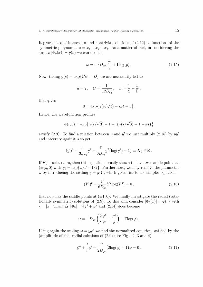
It proves also of interest to find nontrivial solutions of (2.12) as functions of thesymmetric polynomial s = x1 + x2 + x3. As a matter of fact, in considering theansatz |Φ0(x)| = y(s) we can deduce
ω = −3Dqqy′′
y+ Γlog(y) . (2.15)
Now, taking y(s) = expCsa +D we are necessarily led to
a = 2 , C =Γ
12Dqq
, D =1
2+ω
Γ,
that gives
Φ = expγ(s/√
3)− iωt− 1.
Hence, the wavefunction profiles
ψ(t, q) = expγ(s/√
3)− 1 + i(γ(s/√
3)− 1− ωt)
satisfy (2.9). To find a relation between y and y′ we just multiply (2.15) by yy′
and integrate against s to get
(y′)2 +ω
3Dqq
y2 − Γ
6Dqq
y2(log(y2)− 1
)≡ K0 ∈ R .
If K0 is set to zero, then this equation is easily shown to have two saddle points at(±y0, 0) with y0 = expω/Γ + 1/2. Furthermore, we may remove the parameterω by introducing the scaling y = y0Y , which gives rise to the simpler equation
(Y ′)2 − Γ
6Dqq
Y 2log(Y 2) = 0 , (2.16)
that now has the saddle points at (±1, 0). We finally investigate the radial (rota-tionally symmetric) solutions of (2.9). To this aim, consider |Φ0(x)| = ϕ(r) withr = |x|. Then, ∆x|Φ0| = 2
rϕ′ + ϕ′′ and (2.14) does become
ω = −Dqq
(2
r
ϕ′
ϕ+ϕ′′
ϕ
)+ Γlog(ϕ) .
Using again the scaling ϕ = y0φ we find the normalized equation satisfied by the(amplitude of the) radial solutions of (2.9) (see Figs. 2, 3 and 4)
φ′′ +2
rφ′ − Γ
2Dqq
(2log(φ) + 1
)φ = 0 . (2.17)

16 2.4. Numerical evidence accounting for negative dissipation in the log–law Schrodinger equation
2.4 Numerical evidence accounting for negative
dissipation in the log–law Schrodinger equa-
tion
The purpose of this section is to construct numerical solutions of Eq. (2.13)in 1D ( wich is gauge-equivalent to Eq. (2.10) acording to the transformation(2.2) ) and compare them to the exact ones, which come out after solving the(linear) quantum Fokker–Planck master equation in the free particle and dampedharmonic oscillator cases (i.e. Eq. (2.1)–(2.2) with V = 0 and V = 1
2ω2
0x2,
respectively, ω0 denoting the frequency of the oscillator), namely
Wt + ξWx =Dpp
m2Wξξ + 2λ(ξW )ξ +
2Dpq
mWξx +DqqWxx , (2.18)
Wt + ξWx − ω20xWξ =
Dpp
m2Wξξ + 2λ(ξW )ξ +
2Dpq
mWξx +DqqWxx , (2.19)
where subscripts of the Wigner function denote the variables with respect towhich differentiation is performed here and hereafter. To this aim we still choosea unit system for which ~ = m = kB = 1 and adapt the discretization procedureintroduced in [86] to our context. We start with the presentation of the exactsolutions of Eq. (2.19).
2.4.1 Exact solutions of the quantum Fokker–Planck mas-ter equation
Using the standard Fourier transform techniques for the calculus of the propaga-tors Gfr
0 and Gho0 associated with Eqs. (2.18) and (2.19), we obtain the following
expressions (see Appendix A in [71] for the details)
Gfr,ho0 (x, ξ, t) =
1
2π√dfr,ho(t)
exp
− cfr,ho(t)dfr,ho(t)
x2 +bfr,ho(t)
dfr,ho(t)mxξ − afr,ho(t)
dfr,ho(t)m2ξ2
,
where
afr(t) =Dpp
4λ2+Dqq +
Dpq
λ+
1− e−2λt
16λ3
(Dpp
4λ(e−2λt − 3)− 8λDpq
),
bfr(t) =1− e−2λt
4λ2
(4λDpq +Dpp(1− e−2λt)
),
cfr(t) =Dpp
4λ(1− e−4λt) ,
dfr(t) = dho(t) = 4a(t)c(t)− b(t)2 > 0 , ∀ t > 0 ,

2. A wavefunction description of stochastic–mechanical Fokker–Planck dissipation 17
and where
aho(t) =e−4λt
(λ+ − λ−)2
a(t)
(λ+e
λ+t − λ−eλ−t)2
+ c(t)(eλ+t − eλ−t
)2
+ b(t)(λ+e
2λ+t + λ−e2λ−t − 2λe2λt
),
bho(t) = − e−4λt
(λ+ − λ−)2
ω2
0 a(t)(λ+e
2λ+t + λ−e2λ−t − 2λe2λt
)+ c(t)
(λ−e
2λ+t + λ+e2λ−t − 2λe2λt
)+ b(t)
(2ω2
0
(e2λ+t + e2λ−t
)+ (λ+ + λ−)2e2λt
),
cho(t) =e−4λt
(λ+ − λ−)2
a(t)
(eλ+t − eλ−t
)2+ c(t)
(λ+e
λ−t − λ−eλ+t)2
+ω20 b(t)
(λ+e
2λ−t + λ−e2λ+t − 2λe2λt
).
Here, we denoted λ± = λ±√λ2 − ω2
0 and
a(t) =λ2
+
2λ−
[Dqq +
λ−ω2
0
(λ−ω2
0
Dpp + 2Dpq
)](e2λ−t − 1)
+λ2−
2λ+
[Dqq +
λ+
ω20
(λ+
ω20
Dpp + 2Dpq
)](e2λ+t − 1)
− 1
λ
(2ω2
0Dqq +Dpp + 4λDpq
)(e2λt − 1) ,
b(t) =1
λ(2ω2
0Dqq +Dpp + 4λDpq)(e2λt − 1)
−(ω2
0
λ+
Dqq +λ+
ω20
Dpp + 2Dpq
)(e2λ+t − 1)
−(ω2
0
λ−Dqq +
λ−ω2
0
Dpp + 2Dpq
)(e2λ−t − 1) ,
c(t) =ω2
0
2
(ω2
0
λ+
Dqq +λ+
ωDpp + 2Dpq
)(e2λ+t − 1)
+
(ω2
0
λ−Dqq +
λ−ω2
0
Dpp + 2Dpq
)(e2λ−t − 1)
− 1
λ(2ω2
0Dqq +Dpp + 4λDpq)(e2λt − 1)
.
Then, the unique solution to the initial value problem associated with Eqs. (2.18)and (2.19) (the initial datum being W (t = 0, x, ξ) = WI(x, ξ)) is written as
Wfr,ho =
∫R2
Gfr,ho0
(t, x− Afr,hoz (t)z − Afr,hov (t)v,m ξ −Bfr,ho
z (t)z −Bfr,hov (t)v
)×WI(z, v) dvdz,

18 2.4. Numerical evidence accounting for negative dissipation in the log–law Schrodinger equation
where the position and momentum time paths are now given by
Afrz ≡ 1 , Ahoz (t) =1
λ+ − λ−(λ+e
−λ−t − λ−e−λ+t),
Afrv (t) =1− e−2λt
2λ, Ahov (t) =
1
λ+ − λ−(e−λ−t − e−λ+t
),
Bfrz ≡ 0 , Bho
z (t) =ω2
0
λ+ − λ−(e−λ+t − e−λ−t
),
Bfrv = e−2λt , Bho
v (t) =1
λ+ − λ−(λ+e
−λ+t − λ−e−λ−t).
We remark that all of the above calculations also make sense in the complex planewhether λ2 − ω2
0 < 0.
2.4.2 The numerical algorithm
In this paragraph we shall give a short description of the numerical procedure(adapted from that in [86]) employed to approximate the solution to the 1D initialvalue problem associated with Eq. (2.9) as well as its macroscopic magnitudes,say the energy and local and current densities, and dispersion quantities such asthe variance of the wave packet, to be compared with those obtained from theexact Wigner–Fokker–Planck solutions established in the previous section.
Consider the interval [a, b] and the partition associated with the position steph = (b−a)/N . Let also X = xm1≤m≤N+1 and Y = yn0≤n≤N−1 the meshes forthe subsequent evaluations of ψ and ∇xψ respectively, with xm = a + h(m − 1)and yn = xn + h/2 = (xn+1 + xn)/2, equipped with the following inner products
〈u, v〉X =N∑m=0
αmu(xm)v(xm) , 〈u, v〉Y =N−1∑n=0
αmU(yn)Anv(yn) ,
where α = (h, . . . , h)N+1 and A = (h, . . . , h)N . Then, the derivatives (gradientand divergence) can be written as
∇Du(yn) =N+1∑m=1
Dnmu(xm) , ∇D · U(xm) = − 1
αm
N∑n=1
DnmAnU(yn) ,
thus satisfying the essential ’discrete divergence property’
〈u,∇D · V 〉X = −〈∇Du, V 〉Y .
Then, if choosing centered differences ∇u(yn) = 12h
(u(xn+1) − u(xn)
)we are led
to
D = (Dnm)1≤n≤N,1≤m≤N+1 =
− 1h
1h
0 0 . . . 00 − 1
h1h
0 . . . 0
0 0. . . . . . 0 0
......
.... . . . . .
...0 0 0 0 − 1
h1h
,

2. A wavefunction description of stochastic–mechanical Fokker–Planck dissipation 19
so that
∇Du = D
u(x1)u(x2)
...u(xN+1)
,
∇D · U =
1α1D11
1α1D21 . . . 1
α1DN1
1α2D12
1α2D22 . . . 1
α2DN2
......
......
1αN+1
D1(N+1) . . . . . . 1αN+1
DN(N+1)
A1U(y1)A2U(y2)
...ANU(yN)
=
− 1h2 0 0 0 . . . 01h2 − 1
h2 0 0 . . . 0
0. . . . . . 0 . . . 0
......
. . . . . . . . ....
0 0 0 1h2 − 1
h2 0
hU(y1)hU(y2)
...hU(yN)
,
in such a way that
∇ · U(x1) =1
hU(y1) , ∇ · U(xN+1) = −1
hU(yN) ,
∇ · U(xm) =1
h
(U(ym)− U(m− 1)
)∀ 2 ≤ m ≤ N ,
∆Du(xm) =1
h2
(u(xm+1)− 2u(xm) + u(xm−1)
), ∀ 0 ≤ m ≤ N − 1 .
Furthermore, we consider
δtuk =
1
dt(uk+1 − uk) , µtu
k =1
2(uk+1 + uk) ,
where dt denotes the time step. After all this, the discretized version of Eq. (2.9)reads
iδtψk +Dqqµt∆Dψ
k − µtUkµtψk = 0 , (2.20)
where we denoted U(ψ) = 2DqqQ + 12Dqq
(V + Λlog(n)
)+ 1
2
(iDqq
∆xnn
+ ∇x · Jn).
Equivalently, Eq. (2.20) can be rewritten as
i
dt
(ψk+1−ψk
)+Dqq
2
(∆Dψ
k+1 +∆Dψk)− 1
4
(Uk+1 +Uk
)(ψk+1 +ψk
)= 0 . (2.21)
To make this finite differences scheme more tractable form a computational view-point, we invoke a predictor–corrector procedure ψk 7→ ψk,1 7→ ψk+1, where theprediction ψk,1 is obtained from
i
dt
(ψk,1 − ψk
)+Dqq
2
(∆Dψ
k,1 + ∆Dψk)− 1
2Uk(ψk,1 + ψk
)= 0 . (2.22)

20 2.4. Numerical evidence accounting for negative dissipation in the log–law Schrodinger equation
Then we make
Uk,1 :=1
2Dqq
(V + Λlog(nk,1)
)and solve
i
dt
(ψk,2 − ψk
)+Dqq
2
(∆Dψ
k,2 + ∆Dψk)− 1
4
(Uk,1 + Uk
)(ψk,2 + ψk
)= 0 . (2.23)
to find ψk+1 := ψk,2. It is important to note that the whole scheme presentedabove is mass–preserving.
To proceed with the calculations, we make use of an algorithm for an efficientmultiplication of tridiagonal matrices, in such a way that the predictor step ψk,1
is obtained as a solution to Apψk,1 = Bpψ
k, with
Ap =
A1d1 A1c1
A1a2 A1d2 A1c2
. . . . . . . . .
A1aN A1dN A1cNA1aN+1 A1dN+1
,
Bp =
B1d1 B1c1
B1a2 B1d2 B1c2
. . . . . . . . .
B1aN B1dN B1cNB1aN+1 B1dN+1
,
while the corrector step stems from the homologous equation Acψk,2 = Bcψ
k,1,with
Ac =
A2d1 A2c1
A2a2 A2d2 A2c2
. . . . . . . . .
A2aN A2dN A2cNA2aN+1 A2dN+1
,
Bc =
B2d1 B2c1
B2a2 B2d2 B2c2
. . . . . . . . .
B2aN B2dN B2cNB2aN+1 B2dN+1
.

2. A wavefunction description of stochastic–mechanical Fokker–Planck dissipation 21
Here, the various coefficients are given by
A1d1 =i
dt− Dqq
2h2− 1
2Uk
1 , A1d2 =i
dt− 3Dqq
4h2− 1
2Uk
2 ,
A1dN =i
dt− 3Dqq
4h2− 1
2UkN , A1dN+1
i
dt− Dqq
2h2− 1
2UkN+1 ,
A1dn =i
dt− Dqq
h2− 1
2Ukn ∀ 3 ≤ n ≤ N − 1 ,
A1cn =Dqq
2h2∀ 1 ≤ n ≤ N − 1 , A1cN =
Dqq
4h2,
A1a2 =Dqq
4h2, A1an =
Dqq
2h2∀ 3 ≤ n ≤ N + 1 ,
B1d1 =i
dt+Dqq
2h2+
1
2Uk
1 , B1d2 =i
dt− 3Dqq
4h2+
1
2Uk
2 ,
B1dN =i
dt+
3Dqq
4h2+
1
2UkN , B1dN+1 =
i
dt+Dqq
2h2+
1
2UkN+1 ,
B1dn =i
dt+Dqq
h2+
1
2Ukn ∀ 3 ≤ n ≤ N − 1 ,
B1cn = −Dqq
2h2∀ 1 ≤ n ≤ N − 1 , B1cN = −Dqq
4h2,
B1a2 = −Dqq
4h2, B1an = −Dqq
2h2∀ 3 ≤ n ≤ N + 1 .
The matrices A2 and B2 are identical by just replacing 12Ukn by 1
4
(Uk,1n + Uk
n
)for
all 1 ≤ n ≤ N + 1.We now observe that the discretizations of the Doebner–Goldin terms con-
forming the nonlinear potential U(ψ) are given by(log(n)
)k
= log(nk) ∀ 1 ≤ k ≤ N + 1 ,
and Vk =ω2
0
2x2k for all 1 ≤ k ≤ N + 1 (in the harmonic oscillator case). On one
hand, ∇xψ must be evaluated over the mesh Y , ∇xψ(yk) = 1h(ψk+1 − ψk). On
the other hand, as ψ(yk) is not known, we can aproach it by 12(ψk+1 + ψk).
The simulations of the dissipative behaviour of solutions to the free-particuleand harmonic-oscillator logarithmic Schrodinger equation (2.13) are attached atthe end of the Chapter.
2.5 Summary and conclusions
In many mathematical and physical situations the Schrodinger picture of quan-tum mechanics is preferable to the Liouvillian representation, for instance forcomputational reasons. Indeed, the Wigner function is evaluated in the position–momentum space, which makes the subsequent numerical analysis certainly in-tricate. Even from an analytical viewpoint, though most PDE techniques are

22 2.5. Summary and conclusions
expected to be inhereted from kinetic theory, the fact that the probability dis-tribution (i.e. the Wigner function) can assume negative values constitutes aserious drawback in making things rigorous. In any case, it seems convenientto have an ’equivalent’ description of the dissipative Fokker–Planck mechanism,that has proved to give satisfactory results in both the Wigner and the quantumhydrodynamic formulations, in terms of the particle wavefunction. Actually, thatis our main purpose and goal here. Starting from the quantum Fokker–Planckmaster equation, which models the interactions occurring between the electronensemble under examination and the phonons of a thermal bath in the frameworkof open quantum systems, we derive a nonlinear dissipative Schrodinger equationwhich is characterized in an essential way by the presence of a quantum correctionof logarithmic type (present in the literature since the seminal works by Kostin[66] and Bialynicki–Birula and Mycielski [20]) as well as of various other nonlin-earities that fit the Doebner–Goldin diffusive structure [42]. This equation doesretain the same macroscopic local density that the Wigner–Fokker–Planck equa-tion we started with. The derivation follows the fundamental lines of Nelsonianstochastic mechanics [81] combined with Madelung theory [75]. The stationaryregime for the new Eq. (2.9) has been widely explored from both an analyticaland computational point of view, making especial emphasis on the behaviour ofradial solutions and the absence of Gaussons.
Some final remarks on the role played by α are in order. The parameterα = 2mDqq has the dimensions of an action but it is not an universal constant,as it hinges on the particular system under study. Thus, though α 6= ~ in generalit plays the role of ~ in some sense (see [32] for a wider discussion), confering
quantum–mechanical meaning to our wavefunction. If we consider ψ =√n e
i~S
instead of ψ (cf. (2.8)), the continuity equation and Eq. (2.7) along with thequantization rule lead us to
i~∂tψ = Hψ+
(2α2
~2− 1
)Qψ+Λlog(n)ψ+Dqq
(i~2
∇2qn
n+m∇q ·
J
n
)ψ , (2.24)
that might be simplified into the so–called modular Schrodinger equation withcoupling parameter κ = 1− α2
~2 augmented by a logarithmic nonlinearity
iα∂tφ = Hαφ− κQφ+ Λlog(n)φ , (2.25)
by making use of the gauge transformation
g : ψ 7→ φ = ψ exp
− iα
2~log(n)
.
For κ = 1 (see [11, 51]), this equation does not admit exponentially confinedsolutions but it can be derived from a local Lagrangian. Besides, its associatedhydrodynamics does not contain quantum effects. As we have already observed,in Eq. (2.7) the effects derived from the action of Q are quite close to be neg-ligible. On the contrary, the choice of ψ as envelope wavefunction still retains
2. A wavefunction description of stochastic–mechanical Fokker–Planck dissipation 23
this contribution in Eq. (2.25) with κ ' 1. However, taking α as the actionunit makes Q not to appear in Eq. (2.12). Since we are mainly interested in thelocal densities associated with Ψ and ψ, which are identical to each other andalso to that stemming from the Wigner function, we are called to focus furtheranalysis on the simpler Eq. (2.9) and its gauge reduction to the purely loga-rithmic Schrodinger equation (see [59]) . Anyway, both Eqs. (2.9) and (2.24)retain the dissipative effects introduced by the QFPME. Numerical simulationswhen quantum Fokker–Planck dynamics with negative dissipation is reproducedare performed and compared with the exact results for the free particle and thedamped harmonic oscillator cases.

24 2.5. Summary and conclusions
Y
Y’
0 1 2 3−1
−0.5
0
0.5
1
Y
Y’
0 1 2 30
−0.5
0
0.5
1
Y
Y’
0 1 2 3−1
−0.5
0
0.5
1
Y
Y’
0 1 2 3−1
−0.5
0
0.5
1
Figure 2.2: Left to right and top to bottom: the first two pictures show the phaseportrait of (2.16) for typical high–temperature values of the coefficients (T,Ω, λ) withinDekker’s phenomenology [39, 84]: (2, 1, 0.01) and (2, 1, 0.5), respectively. The last twopictures correspond to the opposite sign for the logarithmic term.

2. A wavefunction description of stochastic–mechanical Fokker–Planck dissipation 25
0 0.05 0.1 0.15 0.2 0.25 0.3 0.35 0.4 0.45 0.5
0.05
0.1
r
z
0 0.05 0.1 0.15 0.2 0.25 0.3 0.35 0.4 0.45 0.5
0.05
0.1
0.15
0.2
r
z
Figure 2.3: Numerical solutions of Eq. (2.17) for high temperatures: T = 2, Ω = 1.On the left : V = 0 and λ = 0.2 (dashed), λ = 0.1 (continuous) and λ = 0.01 (dashed-points). On the right: V = w2
0x2/2, w0 = 0.05 and λ = 0.15 (dashed), w0 = 0.3 and
λ = 0.05 (continuous) and w0 = . Left to right: initial data (φ(0) = 0.1, φ′(0) = 0) and(φ(0) = 0.2, φ′(0) = 0), respectively.
0 5 10 15 20 25 30
0.25
0.5
t
E
0 5 10 15 20 25 30
1
2
3
4
5
t
∆ x
Figure 2.4: Position dispersion of the numerical solutions of Eq. (2.10) for high tem-peratures: T = 2, Ω = 1. On the left : V = 0 and λ = 0.1 (dashed), λ = 0.15(continuous). On the right: V = w2
0x2/2, w0 = 0.5 and λ = 0.1 (dashed) and λ = 0.15
(continuous).

26 2.5. Summary and conclusions
0 5 10 15 20 25 305
10
15x 10−3
t
E
0 5 10 15 20 25 300
1
2
3
t
E
Figure 2.5: Kinetic plus potencial energy of the numerical solutions of Eq. (2.10) forhigh temperatures: T = 2, Ω = 1. On the left : V = 0 and λ = 0.1 (dashed), λ = 0.15(continuous). On the right: V = w2
0x2/2, w0 = 0.5 and λ = 0.1 (dashed) and λ = 0.15
(continuous).

Chapter 3
Global H1 solvability of the 3Dlogarithmic Schrodinger equation
3.1 Introduction and main result
The logarithmic Schrodinger equation
i∂ψ
∂t= −D∆ψ + σlog(|ψ|2)ψ , (3.1)
D > 0 being a diffusion constant (typicallyD = ~2m
where ~ is the Planck constantand m stands for the electron mass) and σ ∈ R \ 0 representing the strength ofthe (attractive or repulsive) nonlinear interaction, was proposed by Bialynicki–Birula and Mycielski [20] in 1976 as the only nonlinear equation of Schrodingertype accounting for some fundamental aspects of quantum mechanics such as sep-arability of noninteracting subsystems (i.e. a solution of the nonlinear equationfor the overall system can be constructed by taking the product of two arbitrarysolutions of the nonlinear equations for the subsystems), additivity of the totalenergy for noninteracting subsystems: E[ψ1ψ2] = E[ψ1] + E[ψ2], boundednessfrom below of E[ψ] for a free particle in any number of dimensions, Planck’s rela-tion for all stationary states: E[ψ] = ~ω with ω denoting the frequency, Ehrenfesttheorem and invariance under the transformation ψ 7→ αψexp
(− iσtlog(|α|2)
).
Nevertheless, they only addressed the case σ < 0. A derivation of this equationfrom Nelson’s stochastic quantum mechanics [81] was also given by Lemos in [68](see also [79]). The single sign choice for the logarithmic term first made in [20]and later continued in [27, 28, 29] was owing to the fact that the other sign leadsto an energy functional not bounded from below. However, the positive sign forthe logarithmic nonlinearity was physically justified by Davidson in [35] as rep-resenting a diffusion force within the context of stochastic quantum mechanics.Indeed, by considering slowly varying profiles in the absence of external forcesone easily observes that the kinetic contribution
∫R3 |∇ψ|2 dx is negligible, so that
27

28 3.1. Introduction and main result
the effective energy operator may be written as
E[ψ] = σ
∫R3
|ψ|2log(|ψ|2) dx . (3.2)
This expression is not bounded from below. However, provided ψ(t, x) has itssupport over a domain Ω with finite measure in configuration space, it is a simplematter to check that (3.2) admits a minimizer.
Various meaningful physical interpretations have been given to the presence ofthe logarithmic potential log(|ψ|2) in the Schrodinger equation. Indeed, it can beunderstood as the effect of statistical uncertainty or as the potential energy asso-ciated with the information encoded in the matter distribution described by theprobability density |ψ(t, x)|2. Recently, Eq. (3.1) has proved useful for the model-ing of several nonlinear phenomena including capillary fluids [38] and geophysicalapplications of magma transport [37], as well as nuclear physics [63], Browniandynamics or photochemistry. From a mathematical viewpoint this model hasnot apparently raised much interest, although important contributions have beendone by Cazenave [27, 28], who showed the existence of stable, localized non-spreading profiles of Gaussian shape (Gaussons), Cazenave and Haraux [29] andby Cid and Dolbeault [30], who established some dispersion and asymptotic sta-bility properties via rescaling techniques. Concerning well–posedness, the global–in–time existence of solutions was studied in [27, §9.3] on a subspace of H1
0 (Ω), Ωbeing an arbitrary open domain. Also Jungel, Mariani and Rial dealt in a recentpaper [64] with the local well–posedness in H2(Ω) of the Schrodinger equationequipped with a general family of nonlinearities, among them that of logarithmictype. The locality of their result is owing to the strong constraint imposed byworking with the functional space
Xδ =ψ ∈ H2(Ω) : essinf
x∈Ω|ψ(x)| > δ > 0
in order to avoid the singularity of the logarithmic potential at the origin. In [70],one of us stressed the relevance of a family of logarithmic Schrodinger equations(of Doebner–Goldin type, see [42]) accounting for diffusion currents in appropri-ately modeling quantum dissipation (σ > 0) of an electron ensemble in contactwith a heat bath, when viewed as a hydrodynamic or stochastic approach tothe so–called Wigner–Fokker–Planck equation (see also [8, 71]). In that context,the logarithmic nonlinearity corresponds to a linear velocity–dependent frictionalforce caused by the interaction of the particle ensemble with a dissipative envi-ronment. Other nonlinear Schrodinger models of logarithmic type have provedinteresting in the literature, for instance the Schrodinger–Langevin equation [66]for the description of nonconservative quantum systems or the logarithmic–typeand modular corrections introduced by Sabatier in [89]. In the general settingof nonlinear Schrodinger equations, many different well–posedness results can befound in the literature (see for example [26, 52, 73]), but none of them includesthe model under study here to the best of our knowledge.

3. Global H1 solvability of the 3D logarithmic Schrodinger equation 29
Our aim in this Chapter is to prove the existence of a unique global–in–timemild solution in H1(R3) of the following initial value problem
i∂ψ
∂t= −D∆ψ + σlog(n)ψ , (t, x) ∈ [0,∞)× R3 , (3.3)
ψ(0, x) = ψ0(x) , ψ0 ∈ H1(R3) , |x|n0 ∈ L1(R3) , (3.4)
under the only hypothesis that the initial inertial momentum∫
R3 |x|n0 dx is fi-nite, independently of the fact that attractive or repulsive interactions are con-sidered, where n(t, x) = |ψ(t, x)|2 is the charge density and where we denotedn0(x) = n(0, x). Our main goal consists in developing a mathematical theory ofglobal well–posedness in the whole space consistent in H1(R3), with neither anyrestriction of the functional space in order to avoid the singularity of the loga-rithmic potential at the origin nor technical conditions which allow to guaranteea priori the convergence of the sequence of approximate solutions. Our maintheorem is the following
Theorem 1.3 There exists a unique function
ψ ∈ L∞([0,∞);H1(R3)) ∩ C([0,∞);L2(R3))
which solves the initial value problem (3.3)–(3.4) in a mild sense.
The key points to control the H1–norm are the Carleman entropy inequalityand the logarithmic Sobolev inequality (see (3.14) and (3.21) below) along withthe charge and energy conservations. These inequalities allow us to work in thesubspace of H1 given by the functions with bounded inertial momentum (whichis a natural condition with straightforward mathematical and physical meanings)instead of the subspace consisting of functions with finite energy (which is math-ematically more involved because of the singularity of the potential). Actually,we shall prove that solutions with bounded inertial momentum have finite en-ergy. Our crucial technical goals are the estimates of Lemma 2.2 (i), which donot hold if working only with H1(R3)–solutions. For the sake of selfconsistency,we present in detail the regularization process of our initial value problem in H2
(thus in L∞) and later use some adequate compactness properties.We structure this Chapter as follows: In Section 2 we build up a sequence of
ε–approximate problems via regularization of the logarithmic nonlinearity, each ofthem enjoying global H2(R3) solvability. Finally, Section 3 concerns the passageto the limit ε→ 0 via compactness arguments and the uniqueness proof.
3.2 Global well–posedness of a sequence of ap-
proximate problems
It is well–known that the Laplace operator is self–adjoint and dissipative onH2(R3), so that iD∆ generates a unitary group of isometries U(t) := eitD∆ on

30 3.2. Global well–posedness of a sequence of approximate problems
L2(R3) which gives rise to the free Schrodinger propagator. We start by definingthe concept of solution to the initial value problem (3.3)–(3.4) we shall deal with.
Definition 2.1 (Mild solution) Given T > 0 and X = H1(R3) or H2(R3),the complex function ψ ∈ C(0, T ;X) is called a mild solution of the logarithmicSchrodinger initial value problem (3.3)–(3.4) if it solves the integral equation
ψ(t, x) = U(t)[ψ0]− iσ∫ t
0
U(t− s)[log(n(s))ψ(s)
]ds , (3.5)
where U(t)[ψ0] is the solution of the linear Schrodinger equation.
In order to circumvent the singularity of the potential at the origin, we startby constructing a sequence of wave functions ψε which solves an ε–approximatefamily of problems, consisting in an appropriate regularization of the nonlinearterm log(n)ψ and of the initial data ψ0.
3.2.1 A priori estimates: ε–local existence
For 1 > ε > 0, we consider a sequence of initial data ψε,0 ⊂ H2(R3) convergingto ψ0 in H1(R3) such that the total charge and the inertial momentum satisfy
‖ψε,0‖2L2(R3) := Qε ≤ Q := ‖ψ0‖2
L2(R3) , (3.6)
and‖|x|nε,0‖L1(R3) := Iε(0) ≤ 2 I0 := 2 ‖|x|n0‖L1(R3) , (3.7)
respectively. We then consider the following sequence of approximate initial valueproblems
i∂ψε∂t
= −D∆ψε + σhε(nε)ψε , (t, x) ∈ [0,∞)× R3 , (3.8)
ψε(0, x) = ψε,0(x) , x ∈ R3 , (3.9)
where nε = |ψε|2 and hε(r) is a smooth function defined on R+0 . Let us briefly
show how this function can be constructed and its main properties.
3.2.2 Approximation of the logarithmic nonlinearity
Consider a function hε ∈ C30([0,∞)) verifying
hε(r) :=
log(2 ε/3) , 0 ≤ r < ε/2 ,
log(r) , ε ≤ r < 1/ε ,
0 , 2/ε ≤ r ,
(3.10)
to be extended to [ε/2, ε] and [1/ε, 2/ε] in such a way that
|hε(r)| ≤ |log(r)| ∀r > 0 . (3.11)

3. Global H1 solvability of the 3D logarithmic Schrodinger equation 31
Then, it is continuously defined in r = 0 and obviously approaches log(r). Wenow define the accumulation function
Hε(r) :=
∫ r
0
hε(s) ds ,
which shall play a crucial role in defining the potential energy operator. Forfurther comparison of the potential energy of the original problem,
∫R3 log(n)n dx,
with that of the ε–approximate solutions, we shall derive some simple but usefulestimates on Hε(r). Taking into account that hε(r) ≥ log(r) if r < 1/ε and startsdecaying to zero afterwards, by simply integrating it becomes a simple matter toobserve that
rlog(r)− r ≤ Hε(r) + r3/2 , r ≥ 0 . (3.12)
Using (3.11) and integrating again one can also observe that
|Hε(r)| ≤ |rlog(r)|+ r , r ≥ 0 . (3.13)
Then, from (3.13) we have
Hε(r) ≤ |rlog(r)|+ r = −|rlog(r)|+ 2|rlog(r)|+ r , r ≥ 0 ,
from which, taking into account Carleman’s entropy inequality (see [82])
|rlog(r)| ≤ rlog(r) + |x|r + 2e−|x|/4 (3.14)
and the fact that rlog(r) ≤ r3/2 we finally find
|rlog(r)| ≤ −Hε(r) + 2 r3/2 + (1 + 2|x|)r + 4 e−|x|/4 , r ≥ 0 . (3.15)
These inequalities are far from been optimal and might be easily improved, butare good enough for our purposes here.
3.2.3 ε–local existence
In the sequel, we are intended to apply the standard Pazy’s theory to obtaina global mild solution of the approximate problem (3.8)–(3.9) in H2(R3) (seeTheorem 6.1.4 in [83]). To this purpose, we first show that the nonlinear term islocally Lipschitz continuous in H2(R3), uniformly on bounded intervals of time,i.e. that the operator
Γ : C([0, T ];H2(R3)) → C([0, T ];H2(R3))ψ 7→ hε(|ψ|2)ψ
restricted to
BM :=ψ ∈ H2(R3) : sup
0≤t≤T‖ψ(t)‖H2(R3) ≤M

32 3.2. Global well–posedness of a sequence of approximate problems
is a Lispschitz continuous map for any T > 0 and M > 0. In the following, Cwill represent a generic constant eventually depending on T and M , while Cεwill denote a generic constant depending on ε. Also, for the sake of simplicitywe shall omit further reference to R3 when dealing with the functional spacesL2(R3), H1(R3) or H2(R3). We first compute
‖Γ[ψ1]− Γ[ψ2]‖L2 ≤ ‖hε(|ψ1|2)(ψ1 − ψ2)‖L2 + ‖(hε(|ψ1|2)− hε(|ψ2|2)
)ψ2‖L2
≤ Cε(‖ψ1 − ψ2‖L2 +
∥∥|ψ1|2 − |ψ2|2∥∥L2 ‖ψ2‖L∞
)≤ Cε(1 + 2M2)‖ψ1 − ψ2‖L2 , (3.16)
where we used that ψ ∈ BM implies ‖ψ(t)‖L∞ ≤ C‖ψ(t)‖H2 ≤ CM and the factthat hε is a bounded, Lipschitz continuous function (with a Lipschitz constantdepending on ε). Concerning the gradients, we argue by adding and subtractingseveral crossed terms as follows:
∇Γ[ψ1]−∇Γ[ψ2] = 2h′ε(|ψ1|2)Re(ψ1∇ψ1
)ψ1 + hε(|ψ1|2)∇ψ1
− 2h′ε(|ψ2|2)Re(ψ2∇ψ2
)ψ2 − hε(|ψ2|2)∇ψ2
= 2(h′ε(|ψ1|2)− h′ε(|ψ2|2)
)Re(ψ1∇ψ1
)ψ1
+ 2h′ε(|ψ2|2)Re(ψ1∇ψ1
)(ψ1 − ψ2)
+ 2h′ε(|ψ2|2)Re(ψ1(∇ψ1 −∇ψ2)
)ψ2
+ 2h′ε(|ψ2|2)Re((ψ1 − ψ2
)∇ψ2)
)ψ2
+hε(|ψ1|2)(∇ψ1 −∇ψ2)
+(hε(|ψ1|2)− hε(|ψ2|2)
)∇ψ2 .
Using now that h′ε is also a bounded, Lipschitz continuous function we can esti-mate (term by term) the above expression as follows
‖∇Γ[ψ1]−∇Γ[ψ2]‖L2 ≤ Cε‖ψ1‖2L∞‖∇ψ1‖L4‖ψ1 − ψ2‖L4
+Cε‖ψ1‖L∞‖∇ψ1‖L4‖ψ1 − ψ2‖L4
+Cε‖ψ1‖L∞‖ψ2‖L∞‖∇ψ1 −∇ψ2‖L2
+Cε‖ψ2‖L∞‖∇ψ2‖L4‖ψ1 − ψ2‖L4
+Cε‖∇ψ1 −∇ψ2‖L2
+Cε‖∇ψ2‖L4‖ψ1 − ψ2‖L4
≤ Cε‖ψ1 − ψ2‖H2 . (3.17)
Finally, for the second order derivatives we compute
∆Γ[ψ] = 4h′′ε(|ψ|2)(Re(ψ∇ψ
))2ψ + 2h′ε(|ψ|2)|∇ψ|2ψ
+ 2h′ε(|ψ|2)Re(ψ∆ψ
)ψ + 4h′ε(|ψ|2)Re
(ψ∇ψ
)∇ψ + hε(|ψ|2)∆ψ .
Proceeding as for the gradients, we can analogously estimate ∆Γ[ψ1] − ∆Γ[ψ2]after adding and subtracting various crossed terms in such a way that all pieces
3. Global H1 solvability of the 3D logarithmic Schrodinger equation 33
of the whole estimate involve a difference between ψ1 and ψ2 or their derivatives.For the reader’s convenience, we shall not write up the twenty terms conformingthe whole estimate. In spite of that, we just remark that in all of them the factorsinvolving hε, h
′ε and h′′ε or ψ1 and ψ2 (without derivatives) can be bounded by
their L∞ norm. On the other hand, the gradients of the wave functions can beestimated by their L4 norms and the laplacians by their L2 norms, taking intoaccount in the latter case that the rest of factors in these terms belong to L∞.After all that, we finally get
‖∆Γ[ψ1]−∆Γ[ψ2]‖L2 ≤ Cε‖ψ1 − ψ2‖H2 . (3.18)
Combining now (3.16), (3.17) and (3.18) we achieve the local Lipschitz continuityof the operator Γ in H2(R3):
sup0≤t≤T
‖Γ[ψ1]− Γ[ψ2]‖H2 ≤ Cε sup0≤t≤T
‖ψ1 − ψ2‖H2 , ∀ψ1, ψ2 ∈ BM .
Then, Pazy’s theory applied to (3.8)–(3.9) gives us the existence of a unique mildε–approximate solution
ψε(t, x) = U(t)[ψε,0(x)
]− iσ
∫ t
0
U(t− s)[Γ[ψε(s, x)]
]ds , (3.19)
defined on [0, tmax), where tmax is the maximal time of existence, which equalsinfinity if and only if ‖ψε(t)‖H2 does not blow–up in finite time.
3.2.4 A posteriori estimates: ε–global existence
The required a posteriori estimates and conservation laws for the problem (3.8)–(3.10) before going to the limit ε→ 0 are collected in the following
Lemma 2.1 Let T > 0 and ψε ∈ C(0, T ;H2(R3)) be a mild solution of (3.8)–(3.10). Then, the following properties are fulfilled:
(i) The total charge is preserved along the evolution, i.e.
Qε(t) := ‖ψε(t)‖2L2 = Qε(0) := Qε ≤ Q .
(ii) The inertial momentum satisfies the estimate
Iε(t) := ‖|x|nε(t)‖L1 ≤ C + 2D√Q
∫ t
0
‖∇ψε(s)‖L2 ds ,
where C > 0 is a constant only depending upon the initial data.
(iii) ‖nεhε(nε)‖L1 ≤ ‖nεlog(nε)‖L1 ≤ ‖∇ψε(t)‖2L2 + Iε(t) + C.

34 3.2. Global well–posedness of a sequence of approximate problems
(iv) The total energy operator associated with ψε,
Eε(t) := D
∫R3
|∇ψε(t)|2 dx+ σ
∫R3
Hε(nε(t)) dx ,
is well–defined and preserved along the time evolution, i.e. Eε(t) = Eε(0)for all 0 < t < T .
(v) |σ| |nεlog(nε)| ≤ σHε(nε) + 4|σ|(|x|nε + nε + n3/2ε + e−|x|/4) .
Proof. The standard continuity equation linked to (3.8) reads
∂nε∂t
+ div(jε) = 0 , (3.20)
where jε = 2DIm(ψε∇ψε
)is the electric current associated with ψε. Assertion
(i) is a standard property for Schrodinger models and follows from the continuityequation (3.20) after integrating with respect to the position variable (see also(3.6)), meanwhile (ii) stems from multiplying (3.20) by |x|, integrating by partsand using the estimate ‖jε‖L1 ≤ 2D
√Q‖∇ψε(t)‖L2 and (3.7).
To prove (iii) we first recall (cf. (3.11)) that |hε(r)| ≤ |log(r)| for all r > 0,thus the first inequality is inmediately satisfied. For the second inequality wetake essential advantage of the following logarithmic Sobolev inequality (see [45,§8]) ∫
R3
nεlog(nε)(t) dx ≤ ‖∇ψε(t)‖2L2 +Qεlog(Qε) . (3.21)
Finally, combining the estimates (3.14) and (3.21) along with (ii) yields (iii).The total energy operator is well–defined thanks to (3.13), (iii) and (ii), by
simply noting that
|Eε(t)| ≤ D‖∇ψε(t)‖2L2 + |σ| ‖Hε(nε(t))‖L1
≤ C(‖ψε(t)‖2
H1 + ‖nε(t)log(nε(t))‖L1 +Q).
The preservation property stated in (iv) follows from a direct computation on(3.8) by using that ψε ∈ H2, the relation H ′ε(r) = hε(r) and the continuityequation (3.20).
Finally, we prove (v) in two steps concerning the two possible cases σ > 0 andσ < 0. On one hand, if σ > 0 we may use (3.14) which along with (3.12) leads to
|rlog(r)| ≤ Hε(r) + (1 + |x|)r + r3/2 + 2e−|x|/4 ,
hence to (v) by identifying r = nε. On the other hand, if σ < 0 we just multiplyinequality (3.15) times |σ| = −σ to get (v) after identifying again r = nε.
In the following lemma we collect the precise estimates that will yield theglobal–in–time existence in H2 of the ε–approximate mild solutions.

3. Global H1 solvability of the 3D logarithmic Schrodinger equation 35
Lemma 2.2 Let ψε ∈ C(0, T ;H2(R3)) be a mild solution of (3.8)–(3.10). Then,there exist positive constants Cε (independent of time) and C (independent oftime and ε) such that
(i) ‖∇ψε(t)‖L2 +‖nεlog(nε)(t)‖L1 +‖|x|nε(t)‖L1 ≤ CeCT , for all t ≤ T < tmax.
(ii)∥∥∥∂ψε∂t
(t)∥∥∥L2
+ ‖∆ψε(t)‖L2 ≤ CεeCεT , for all t ≤ T < tmax.
(iii) ‖ψε(t)‖H2 ≤ CεeCεT , for all t ≤ T < tmax and tmax =∞.
Proof. Using Lemma 2.1(v), (iv) and (ii), the following estimate
D
∫R3
|∇ψε(t)|2 dx+ |σ|∫
R3
|nεlog(nε)(t)| dx
≤ Eε(t) + 4|σ|∫
R3
(|x|nε + nε + n3/2ε + e−|x|/4) dx
≤ Eε(0) + 4|σ|(C + 2D
√Q
∫ t
0
‖∇ψε(s)‖2L2 ds+ ‖ψε(t)‖3
L3
)≤ C
(1 +
∫ t
0
‖∇ψε(s)‖2L2 ds
)+ 4|σ|‖ψε(t)‖3
L3
holds. Now, interpolation and Sobolev–Gagliardo–Nirenberg inequalities applyto give
‖ψε(t)‖3L3 ≤ ‖ψε(t)‖3/2
L2 ‖ψε(t)‖3/2
L6 ≤ CSGN Q3/2‖∇ψε(t)‖3/2
L2 ,
thus we deduce
D‖∇ψε(t)‖2L2 + |σ|
∫R3
|nεlog(nε)(t)| dx
≤ C(
1 +
∫ t
0
‖∇ψε(s)‖2L2 ds
)+ 4|σ|CSGN Q3/2‖∇ψε(t)‖3/2
L2 . (3.22)
Finally, applying to (3.22) the following inequality from real analysis
r3/2 ≤ 54|σ|3C3SGNQ
9/2
D3+
D
8|σ|CSGN Q3/2r2 , r ≥ 0 ,
with r = ‖∇ψε(t)‖L2 , we conclude
D
2‖∇ψε(t)‖2
L2 + |σ| ‖nεlog(nε)(t)‖L1 ≤ C(
1 +
∫ t
0
‖∇ψε(s)‖2L2 ds
).
Now, the proof of (i) ends after application of Gronwall’s lemma and Lemma2.1(ii).

36 3.3. Passing to the limit ε→ 0: Global solvability in H1(R3)
We now prove (ii). The regularity of ψε along with (3.8) show that ∂tψεbelongs to L2 but do not provide a control of the norm. However, following [27,§5] we can argue as follows, starting from the mild formulation:
ψε(t+ h, x)− ψε(t, x) = i
∫ h
0
U(s)[∆ψε,0(x)] ds
−iσ∫ h
0
U(t+ h− s)[Γ[ψε(s, x)]
]ds
−iσ∫ t
0
U(t− s)[Γ[ψε(s+ h, x)]− Γ[ψε(s, x)]
]ds.
Taking L2 norms, using that U(t) is an isometry in L2 in the tree integrals of theright–hand side and the inequality (3.16) for the third term, we guess that
‖ψε(t+ h)− ψε(t)‖L2 ≤ h(‖∆ψε,0‖L2 + Cε
)+ Cε
∫ t
0
‖ψε(s+ h)− ψε(s)‖L2 ds .
Now, Gronwall’s lemma applies to give us the first part of (ii). The second partis now straightforward by noticing that
∆ψε =1
D
(− i∂ψε
∂t+ σhε(nε)ψε
).
Finally, (iii) is an inmediate consequence of (i) and (ii) as well as of chargeconservation (cf. Lemma 2.1(i)).
Remark 2 Notice that, in spite of the fact that a change of sign in the non-linear term of the logarithmic Schrodinger equation (3.3) generates very differentdynamics (see [70] for a 1D analysis), the a priori and a posteriori estimates de-rived in previous sections to finally achieve the H1(R3) existence of mild solutionsare all independent of the sign choice.
3.3 Passing to the limit ε→ 0: Global solvability
in H1(R3)
We finally find the unique global–in–time solution ψ(t, x) to (3.3)–(3.4) as thelimit of the ε–approximate solutions ψε(t, x) to (3.8)–(3.10), as ε is sent to zero,by means of the following
Theorem 3.4 (Existence) Let ψε be the mild solution of (3.8)–(3.10). Then,there exists a function ψ ∈ L∞([0,∞);H1(R3))∩C([0,∞);L2(R3)) such that, upto a subsequence,
(i) ψε converges to ψ as ε→ 0 in C([0, T ];L2(R3)) for all T > 0,
(ii) ψεhε(nε) converges to ψlog(|ψ|2) as ε→ 0 in L2loc([0,∞)× R3),

3. Global H1 solvability of the 3D logarithmic Schrodinger equation 37
(iii) ψ is a mild solution of the initial value problem (3.3)–(3.4).
Proof. We start by showing that, for 1 ≤ p < 6, the following inequality
‖φhε(|φ|2)‖Lp(K) ≤ ‖φ log(|φ|2)‖Lp(K) ≤ C(1 + ‖φ‖H1(K)) (3.23)
holds for any function φ ∈ H1(K) and any bounded domain K ⊂ R3. To do thatwe recall that, according to (3.11), we only need to prove the second inequality.
First we split φ log(|φ|2) into two parts as φ log(|φ|2) = φ log(|φ|2)(χ|φ|<1 +
χ|φ|≥1
)in such a way that after optimizing we find
|φlog(|φ|2)| ≤ 2
e+ C|φ|1+β ,
where β is any positive number. Given that φ ∈ Lq(K) for all 1 ≤ q ≤ 6, it is asimple matter to conclude (3.23) via Sobolev imbeddings.
We are now in position to prove (i). The charge conservation established inLemma 2.1(i) (cf. (3.6)) guarantees the (a priori, weak∗) convergence of a subse-quence of ψε to a function ψ in L∞([0, T ];L2(R3)) for all T > 0. In order to ob-serve that this convergence is actually strong, and thus that ψ ∈ C([0, T ];L2(R3)),we use Aubin’s Lemma (see [12] or [82, Lemma 11]). We first note that the mo-mentum bounds established in Lemma 2.2(i) guarantee that for all R > 0, wehave ∫
|x|>R|ψε(t, x)|2dx ≤
∫|x|>R
|x|R|ψε(t, x)|2dx ≤ 1
RCeCT , ∀t ∈ [0, T ].
Then, the arbitrariness of R reduces the problem to prove the convergence only inC([0, T ];L2(K)), K being the ball of radius R. Finally, using the kinetic energybound showed in Lemma 2.2(i) together with the inequality (3.23) for ψε andthe approximated equation (3.8), we deduce that the sequence ψε is bounded inL∞([0, T ];H1(K)) and its time derivative ∂ψε
∂tis bounded in L∞([0, T ];H−1(K)).
Therefore, a straightforward application of Aubin’s Lemma concludes the proof.Moreover, the boundedness of ∇ψε directly implies that ψ ∈ L∞([0,∞);H1(R3)).
Let us now prove (ii). We first note that, by according to (3.23), we deducethat
‖ψεhε(|ψε|2)‖L2(K) ≤ C(1 + ‖ψε‖H1) , ‖ψlog(|ψ|2)‖L2(K) ≤ C(1 + ‖ψ‖H1) ,
for any arbitrary bounded domain K ⊂ R3, so they are both in L2loc([0,∞)×R3)
as stated in (ii). To prove the convergence we observe that the sequence of func-tions z 7→ zhε(|z|2) is uniformly equicontinuous on compact sets (although notuniformly Lipschitz continuous), thus we can deduce via Ascoli–Arzela’s theoremthat it converges uniformly on compact sets to zlog(|z|2). Combining this con-vergence property with (i), we easily deduce that ψεhε(nε) tends to ψlog(|ψ|2)

38 3.3. Passing to the limit ε→ 0: Global solvability in H1(R3)
a.e. (t, x) ∈ [0, T ]×K. Using now Egorov’s theorem we find that, for any k ∈ N,there exists a subset A ⊂ [0, T ]×K with measure |A| < 1/k such that ψεhε(nε)converges to ψlog(|ψ|2) uniformly on (t, x) ∈
([0, T ] ×K
)\ A. Therefore, there
exists ε0 > 0 such that for any ε < ε0 we have
‖ψεhε(|ψε|2)− ψlog(|ψ|2)‖L2(([0,T ]×K)\A) ≤√|K|Tk
.
On the other hand, from (3.23) and Holder’s inequality we can compute
‖ψεhε(|ψε|2)− ψlog(|ψ|2)‖L2(A) ≤ 2C|A|1/4 ≤ 2C
k1/4
and conclude that, for any ε < ε0, we have
‖ψεhε(|ψε|2)− ψlog(|ψ|2)‖L2([0,T ]×K) ≤√|K|Tk
+2C
k1/4.
Now we are done with (ii).Finally, (i) and (ii) allow us to go to the limit ε→ 0 in the mild formulation
(3.19) and show that the limiting wave function ψ is a mild solution of (3.3),which completes the proof.
Theorem 3.5 (Uniqueness) Let ψ1, ψ2 ∈ C([0,∞);L2(R3)) be two mild solu-tions of the initial value problem (3.3)–(3.4). Then ψ1 = ψ2 a.e., thus the wholesequence of ε–approximate solutions converges to it.
Proof. We just make a sketch of the proof, since the details can be found in [27].Take u, v ∈ C so that we may assume 0 < |v| < |u| without loss of generality.Then, using the inequality∣∣log(|v|)− log(|u|)
∣∣ ≤ |v − u||v|
along with the identity
|Im(vu− uv)| = |v(u− v) + v(v − u)| ≤ 2|v||v − u|,
the following result is achieved∣∣∣Im((vlog(|v|2)− ulog(|u|2))(v − u)
)∣∣∣ ≤ 4|v − u|2. (3.24)
Computing now the difference between (3.3) and its conjugate counterpart for ψ1
and ψ2 and taking the L2 product with (ψ1 − ψ2), it follows that
d
dt
∫R3
|ψ2 − ψ1|2 dx = 2σIm
(∫R3
(ψ2log(|ψ2|2)− ψ1log(|ψ1|2)
)(ψ2 − ψ1
)dx
).
Then, (3.24) with u = ψ1 and v = ψ2 implies
‖ψ2(t)− ψ1(t)‖2L2 ≤ 8|σ|
∫ t
0
‖ψ2(s)− ψ1(s)‖2L2 ds .
Uniqueness follows after a straightforward application of Gronwall’s lemma. Thiscompletes the proof.

Chapter 4
On the analysis of travellingwaves to a nonlinear flux limitedreaction–diffusion equation
4.1 Introduction and main results
The aim of this Chapter is to analyze the existence of travelling waves associatedto a heterogeneous nonlinear diffusion partial differential equation coupled to areaction term of Fisher–Kolmogorov–Petrovskii–Piskunov type. The nonlineardiffusion term has been motivated in different contexts and from different pointsof view (see the pioneering work [88]). Also, it has been deduced in the Monge-Kantorovich’s optimal mass transport framework where it is usually called therelativistic heat equation [19] or in astrophysics [77]. The existence and unique-ness of entropy solutions for the nonlinear parabolic flux diffusion was provedin [4], while in [5] the finite speed of propagation was analyzed. The resultingreaction–flux–limited–diffusion system exhibits new properties compared to theclassical reaction coupled to the linear diffusion equation, such as the existence ofsingular travelling waves which opens new perspectives of application to biologyor traffic flow frameworks.
Reaction–diffusion systems consist in mathematical models describing the dy-namics of the concentration of one or more populations distributed in space underthe influence of two processes: local reactions in which the populations interactwith each other, and diffusion which provokes the populations to spread out inspace. In the context of reaction-diffusion the notion of population can be under-stood in a wide sense such as particles or concentrations in chemical processes, butalso examples can be found in biology (cells, morphogens), geology, combustion,physics and ecology or more recently in computer science or complex systems,see for instance [31, 47, 61, 74, 76, 78, 90, 92, 94]. This fact has motivated theattention by both formal and rigorous work on a variety of applications starting
39

40 4.1. Introduction and main results
from linear diffusion of type
∂u
∂t= ν ∆u+ f(u), u(t = 0, x) = u0(x), (4.1)
where ν is the so called diffusion coefficient and f represents the reaction term.Cooperative behavior often stems from diffusive coupling of nonlinear elementsand reaction-diffusion equations provide the prototypical description of such sys-tems.
In many applications and in particular in complex systems reaction-diffusionequations often provide a natural mathematical description of these dynami-cal networks since the elements of the networks are coupled through diffusionin many instances. The correct description of reaction-diffusion phenomena re-quires a detailed knowledge of the interactions between individuals and groupsof individuals. This line of research motivates the study of nonlinear cooperativebehavior in complex systems [13], which is a closed subject interconnected withreaction–diffusion systems. There is a wide literature raising the universality ofapplication of reaction–diffusion systems. Nevertheless, there are limitations tothe reaction-diffusion description. In biochemical networks constituted by smallcellular geometries a macroscopic reaction-diffusion model may be inappropriate.In some circumstances the coupling among elements is not diffusive or the diffu-sive processes are nonlinear, which will strongly influence the dynamical behaviorof the network. In [91] it is proposed a nonlinear degenerate density-dependentdiffusion motivated by the fact that there are biological (mating, attracting andrepelling substances, overcrowding, spatial distribution of food, social behavior,etc.) and physical (light, temperature, humidity, etc.) factors which imply thatthe probability is no longer a space-symmetric function, i.e., it looses the ho-mogeneity, and so linear diffusion is not a good approach. This heterogeneityproperty of the diffusion operator comes from the heterogeneous character of theequation and/or from the underlying domain, we refer also to [16, 17, 14, 15]. Thesame problems with the universality in the applicability occurs when we have nota mean-field interaction between particles or when the particles are dilute or largewith respect to the vessel or the media where they are moving [6, 90]. In thesecases the linear diffusion approximation might not be the most appropriate. Theabove processes probably require to incorporate one or various phenomena notincluded in linear diffusion such as the finite speed of propagation of matter or theexistence of nonsmooth densities (singular travelling waves), for example. Themathematical argument justifying that even if the solution has not compact sup-port the size (mass or concentration, depending on the case dealt with) is verysmall out of some ball with large radius could be unrealistic because in severalapplications in biology (morphogenesis) [1, 15, 94, 96], social sciences [13] or traf-fic flow [18] this kind of situations (solutions with large queues) could activateother processes which is the case, for example, of the biochemical processes in-side the cells whose activation depends on the time of exposure as well as on thereceived concentration of morphogen, see [1]. Then, exploring or modeling new

4. On the analysis of travelling waves to a nonlinear flux limited reaction–diffusion equation 41
nonlinear transport/diffusion phenomena is an interesting subject not only fromthe viewpoint of applications but also from a mathematical perspective.
Reaction–diffusion systems have also attracted the attention as prototypemodels for pattern formation which is, in particular, connected with the studyof travelling waves, i.e. solutions of the type u(t, x) = u(x − σt) playing an im-portant role in concrete applications. The problem when considering travellingwaves for (4.1) is that the evolution of the support could have an infinite speedof propagation, which would contradict the fact that the speed should not exceedthe propagation rate of the real transport process.
Motivated by the above considerations the objective of this Chapter consistsin analyzing the existence of travelling waves for the one–dimensional, nonlinear,flux limited reaction–diffusion equation
∂u
∂t= ν∂x
u∂xu√|u|2 + ν2
c2|∂xu|2
+ f(u), u(t = 0, x) = u0(x), (4.2)
where ν is the viscosity and c is a constant velocity related to the inner propertiesof the particles. Why this election for the nonlinear diffusion term? First of all,the solutions to this system have finite speed of propagation as opposite to thelinear heat equation, i.e. for an initial data with compact support the velocityof growth of the support of the solution is bounded by c (see [2]). Furthermore,this is an extension of the heat equation in the following sense: rewrite the heatequation as
∂u
∂t= ν
∂
∂x
[u∂
∂xlnu
]= ν
∂
∂x[u v], (4.3)
where v is a microscopic velocity. In this form the heat equation can be seen asa transport kinetic equation. The velocity v is determined by the entropy of thesystem, S(u) = ulnu, and by the concentration u, via the following formula
v =∂
∂x
(S(u)
u
). (4.4)
Note that S(u)u
= lnu is known as the chemical potential. We propose to modifythe form of the flux in (4.3) by considering a new microscopic velocity averagedwith respect to the line element associated with the motion of the particle, sothat the new velocity is given by ∂
∂v
√1 + |v|2 = v√
1+|v|2with
v =∂x(S(u)/u)√
1 + [∂x(S(u)/u)]2, (4.5)
arriving at the flux limited equation (4.2). This implies that the chemical poten-tial is now finite, which is not the case for the linear heat equation. Thus, thevelocity for which the concentration or density u is transported depends on the

42 4.1. Introduction and main results
entropy of the system (determining the disorder) as well as on its density underan appropriate measure. This is the situation in which one can think in a trafficflow or in a biological context, for example.
For the reaction term, we will consider one canonical model of Fisher [48] orKPP [65] (for Kolmogorov, Petrovsky and Piskunov) type to analyze travellingwaves, called FKPP from now on. For the linear diffusion case, the propertiesassociated with this system are well understood in the homogeneous framework,see for example [9, 10, 48, 65]. The above equation (4.2) with f = 0 is known asthe relativistic heat equation and is one among the various flux limited diffusionequations used in the theory of radiation hydrodynamics [77].
The term f(u) is written as uK(u), where K is known in biology as thegrowth rate of the population. The main hypotheses on the FKPP reaction termK ∈ C1([0, 1]) are typically written as
(i) K(1) = 0 , (ii) K ′(s) < 0 , s ∈ (0, 1] . (4.6)
These hypotheses on K(u) have some consequences on f(u) such us f(0) = f(1) =0, f ′(1) < 0, f ′(0) > 0, f > 0 in (0, 1). Hypothesis (i) in (4.6) is a normalizationproperty of the carrying capacity and (ii) represents a saturation of the mediawhen the concentration is increasing. Typical examples of such nonlinearities areK(s) = k(1 − s) or K(s) = k(1 − s2), where k = K(0) = f ′(0) is a constantrelated to the growth rate of the (biological) particles, usually called intrinsicgrowth rate. In [48, 65] it was proved that, under the above assumptions, there isa threshold value σ∗ = 2
√νk for the speed σ associated with the linear diffusion
system (4.1). Namely, no fronts exist for σ < σ∗, and there is a unique front (upto space or time shifts) for all σ ≥ σ∗.
The study of existence and uniqueness of solutions to the flux limited reaction-diffusion equation (4.2) has been done in [2], see also the references therein fora complete study of the “relativistic” heat equation. The natural concept ofsolution for this problem implies the use of Kruzhkoz’s entropy solutions. In fact,in [2] it is proved that for any initial datum 0 ≤ u0 ∈ L1(RN) ∩ L∞(RN), thereexists a unique entropy solution u of (4.2) in the N -dimensional case [0, T )×RN ,for every T > 0, such that u(t = 0) = u0. In addition, solutions live in a subspaceof Bounded Variation functions. Moreover, if u(t), u(t) are the entropy solutionscorresponding to initial data u0, u0 ∈ (L∞(RN) ∩ L1(RN))+, respectively, then
‖u(t)− u(t)‖L1(RN ) ≤ et‖f‖Lip‖u0 − u0‖L1(RN ) , ∀t ≥ 0 ,
where ‖f‖Lip denotes the Lipschitz constant for f in [0, 1]. The the existence ofentropy solutions to initial data only in in L∞ was extended in Proposition 3.14of [2].
One of the most important differences between the linear (4.1) and the nonlin-ear (4.2) diffusion models emerges, besides the existence theory reported above,in the study of travelling waves. A travelling wave is a solution having a constantprofile which moves with constant speed, i.e. a solution of the equation of the

4. On the analysis of travelling waves to a nonlinear flux limited reaction–diffusion equation 43
form u(t, x) = u(ξ) with ξ = x− σt for some constant σ. The function u is usu-ally called the wave profile and the constant σ is the wave speed. Let us give asimple example that may illustrate the results obtained in this Chapter for (4.2)by means of a simplified reaction-flux–limited-diffusion equation,
∂tu = ∂x
(u∂xu
|∂xu|
)+ u(1− u) , (4.7)
which allows us to compute explicit travelling waves. Given (4.7), the equationsatisfied by a decreasing wave front profile u(ξ) = u(x− σt) is
−σu = −u+ u(1− u) .
Then, it can be easily proved the existence of a unique, global classical solutiongiven by
uσ(ξ) =1
e−1
σ−1ξ + 1
, ξ ∈ R ,
only if σ > 1 up to space or time shifts. Furthermore, the step function u(ξ) =1 if ξ < 0 and null otherwise, gives the travelling wave profile of an entropy solu-tion to (4.7) with σ = 1. Let us observe how regular and discontinuous solutionscoexist in this simplified model. To complete the above results see [2].
As in the previous case, we find singular profiles for the travelling waves of(4.2) which to a certain extent constitute the equivalent notion of shock waves inhyperbolic models for traffic flow. On the other hand, there is a wide variety andsignificant differences for the possible choices of the velocity σ for the travellingwave solutions to the nonlinear reaction–diffusion equations (4.2) with respect tothose associated with (4.1).
In this Chapter, we look for a particular kind of travelling waves called wavefront, determined by a decreasing wave profile u ∈ (0, 1) such that limξ→−∞ u(ξ) =1, limξ→∞ u(ξ) = 0, verifying (4.2) in a sense specified later. By the degeneratecharacter of the flux limiter if u ≡ 0, we split the analysis of the wave front in twosteps. For the positive part u(ξ) > 0 ∀ξ ∈ (−∞, ξ0), we impose that u ∈ C2 solvesthe equation in a classical sense. Thus, if ξ0 =∞ we will have a classical solutionverifying the equation everywhere in the domain of definition. If ξ0 <∞, we willsee that the null extension of the positive part can be an entropy solution undercertain conditions, these solutions being discontinuous. The entropy criterium isnecessary in this problem since it selects travelling waves of discontinuous type.
Our main result is the following.
Theorem 1.6 In terms of a value σ∗ ≤ c, depending on ν, c, and k, there existsa wave front which is
(i) a classical solution to (4.2), with wave speed σ > σ∗ or σ = σ∗ < c;
(ii) a discontinuous entropy solution to (4.2), with wave speed σ = σ∗ = c.

44 4.2. An equivalent problem for classical travelling waves
Remark 3 The existence of travelling wave solutions in the case σ < σ∗ is anopen problem. Also, the existence of other kind of travelling waves such as thosewith pulses or soliton-type shape could be explored, see for example [87] or [44] inanother context.
In Section 2 we will analyze the necessary and sufficient condition for theparameters ν, c, and k in order to determine σ∗. The analytical theory dealingwith the existence of a solution-set-structure follows from the associated asymp-totic initial value problem satisfied by the travelling wave profile. This problemis framed in the analysis of a planar dynamical system where the wave speed σis a parameter.
Another fundamental property of equation (4.1) concerns the asymptoticspeed of spreading and was established in [10]: If u0 ≥ 0 is a continuous functionin RN with compact support and u0 6≡ 0, then the solution u(t, x) with initialdata u(t = 0, x) = u0(x) spreads out with speed σ∗ in all directions as t→ +∞,i.e. max|x|≤σt|u(t, x) − 1| → 0 for each σ ∈ [0, σ∗), and max|x|≥σtu(t, x) → 0 foreach σ > σ∗. A similar result may fit our context by the control of the boundof the entropy solution in the set x > σ t by means of an exponential functionwith negative exponent (see Proposition 3.4 below).
The Chapter is organized as follows. In Section 2 we pose the asymptoticinitial value problem associated with travelling wave solutions and deal with theexistence and uniqueness of regular travelling waves. Finally, in Section 3 weanalyze the singular wave profiles that can be identified as entropy solutions.
4.2 An equivalent problem for classical travel-
ling waves
As we mentioned before, the aim of this section is to analyze the classical wavefront solutions to (4.2).
4.2.1 Travelling wave equations
The existence of a regular travelling wave u(x − σt) of the equation (4.2) leadsto the problem of finding a solution of the following equation
ν
uu′√|u|2 + ν2
c2|u′|2
′ + σu′ + f(u) = 0 , (4.8)
which is defined on (−∞, ξ0) and satisfies
limξ→−∞
u(ξ) = 1 (4.9)
andu′(ξ) < 0 for any ξ ∈ (−∞, ξ0) . (4.10)

4. On the analysis of travelling waves to a nonlinear flux limited reaction–diffusion equation 45
The constant σ is a further unknown of the problem. Let us analyze this asymp-totic initial value problem where f(u) = uK(u) and K fulfills (4.6). The followingresult contributes to deduce the asymptotic value of the derivative of u.
Lemma 2.3 Let u : (−∞, ξ0)→ (0, 1) be a solution of (4.8) that satisfies (4.9)-(4.10). Then,
limξ→−∞
u′(ξ) = 0 . (4.11)
Proof. Take ξn → −∞ with ξn < ξ0. For any fixed n ∈ N we use the meanvalue theorem in the interval [ξn − 1, ξn] to obtain the existence of a sequencesn ∈ [ξn − 1, ξn] satisfying
u′(sn) = u(ξn)− u(ξn − 1)→ 0.
Then, we integrate (4.8) over [sn, ξn] and analyze the terms of the followingequality
∫ ξn
sn
ν
u(δ)u′(δ)√|u(δ)|2 + ν2
c2|u′(δ)|2
′ dδ +
∫ ξn
sn
σu′(δ)dδ +
∫ ξn
sn
f(u(δ))dδ = 0 .
The third term ∫ ξn
sn
f(u(δ))dδ → 0 ,
since the interval is bounded and the integrand converges uniformly to zero. Thesecond term, using Barrow’s rule, is
σ(u(ξn)− u(sn))
that tends to zero because of (4.9). The first term, again from Barrow’s rule,takes the form
νu(ξn)u′(ξn)√
|u(ξn)|2 + ν2
c2|u′(ξn)|2
− ν u(sn)u′(sn)√|u(sn)|2 + ν2
c2|u′(sn)|2
,
which tends to zero since u′(sn)→ 0 and
νu(ξn)u′(ξn)√
|u(ξn)|2 + ν2
c2|u′(ξn)|2
→ 0.
Using (4.10) one gets
u(ξn)u′(ξn)√|u(ξn)|2 + ν2
c2|u′(ξn)|2
=−1√
1|u′(ξn)|2 + ν2
c21
|u(ξn)|2
,

46 4.2. An equivalent problem for classical travelling waves
therefore1
|u′(ξn)|2+ν2
c2
1
|u(ξn)|2→∞ .
As the second term tends to ν2
c2, then 1
|u′(ξn)|2 → ∞ and finally u′(ξn) → 0. We
have then shown that for any ξn → −∞, u′(ξn)→ 0. This proves (4.11).
In a classical framework, looking for travelling wave solutions is equivalentto finding heteroclinic trajectories of a planar system of ODE’s which arisesfrom transforming the original problem into travelling wave coordinates (see[48, 65, 91]). The same ideas in the search of travelling waves of (4.2) leadsto a system which is not uniquely derived from heteroclinic trajectories. Hence,a more detailed analysis of the phase diagram for the planar system of ODE’s isrequired. Define
r(ξ) = −νc
u′(ξ)√|u(ξ)|2 + ν2
c2|u′(ξ)|2
, (4.12)
where u is any positive solution of (4.8)–(4.9)–(4.10). Then (u, r) satisfies thefirst order differential system
u′ = − cν
|u| r√1− r2
,
r′ =c
ν
r(r − σc)
√1− r2
+1
cK(u) .
(4.13)
By using that u′ < 0, (4.12) yields r ∈ (0, 1). Also, Lemma 2.3 implies limξ→−∞ r(ξ) =0. As a consequence, the problem of finding a maximal solution of (4.8)–(4.10) isequivalent to look for a solution (u, r) : (−∞, ξ0)→ (0, 1)2 of (4.13), maximal in(0, 1)2, that satisfies
limξ→−∞
u(ξ) = 1, limξ→−∞
r(ξ) = 0. (4.14)
We now analyze the equilibrium points of the system (4.13) which are (1, 0)and (0, r∗), where r∗ ∈ (0, 1) is a possible root of
c
ν
r(r − σc)
√1− r2
+1
ck = 0 , (4.15)
with k = K(0) = f ′(0). The existence of equilibrium points (u, r) = (0, r∗) willdetermine the behavior of the solution to (4.13)-(4.14) and consequently of thesolution to (4.8)–(4.10). More precisely, we obtain the following result.
Proposition 2.1 There always exists a solution u of (4.8) that satisfies (4.9)and (4.10). This solution is unique up to a time translation and verifies:

4. On the analysis of travelling waves to a nonlinear flux limited reaction–diffusion equation 47
(i) If there exist no roots r∗ ∈ (0, 1) of (4.15), then the existence interval for ucan be extended to (−∞, ξ0), with ξ0 <∞, and
limξ→ξ0
u(ξ) > 0, limξ→ξ0
u′(ξ) = −∞. (4.16)
(ii) If there exist roots of (4.15), then ξ0 =∞ and u satisfies
limξ→∞
u(ξ) = 0 . (4.17)
As a consequence, this solution is maximal in R×(−1, 1) and is located in (0, 1)2.
To prove Proposition 2.1 we will need two preliminary results describing someproperties of r and u.
Lemma 2.4 Let −∞ < ξ0 ≤ ∞ and (u, r) : (−∞, ξ0) → (0, 1)2 be a solutionof (4.13) that satisfies (4.14). Then, r′(ξ) > 0. The same holds true for anyextension of (u, r). In particular, the maximal solution (uM , rM) associated with(u, r) remains in (0, 1)2 and verifies r′M(ξ) > 0.
We will give the proof of this result at the end of this Section by analyzing indetail the zeros of r′ in (4.13) and describing the phase diagram associated with(4.13)-(4.14).
The following result deals with the strict positivity of u.
Lemma 2.5 Let (u, r) : (ξ1, ξ0) → (0, 1)2 be a solution of (4.13), where −∞ ≤ξ1 < ξ0 ≤ ∞ are such that
limξ→ξ0
r(ξ) = 1 , r′(ξ) > 0 .
Thenlimξ→ξ0
u(ξ) > 0 .
Proof. Denote (u, r) this particular solution. A contradiction argument allowsto define u(r) := u(r−1(r)) in an interval (1− ε, 1) that satisfies
z′ =−zr
r(r − σc) + ν
c2K(u(r))
√1− r2
, z(1) = 0 .
If σc6= 1, this equation is locally Lischitsz-continuous in z and the point (1, 0) is
regular. Then, by using the uniqueness of the initial value problem z must vanishidentically, which is a contradiction. If σ
c= 1, then the differential equation is
singular. However, u is a solution of the differential equation
z′ = −z h(r)√1− r

48 4.2. An equivalent problem for classical travelling waves
Withh(r) =
r
−r√
1− r + νc2K(u(r))
√1 + r
.
The term h(r)√1−r is singular but improperly integrable and the associated differential
equation has uniqueness again by arguing via the separated variables theory.
We are now in a position to prove Proposition 2.1.
4.2.2 Proof of Proposition 2.1
A local analysis of (4.13) gives the following Jacobian matrix in (u, r)
J [u, r] =
− cν
r√1− r2
− cν
u
(1− r2)3/2
K ′(u)
c− cν
σc− 2r + r3
(1− r2)3/2
.
Clearly,
J [1, 0] =
0 − c
ν
K ′(1)
c−σν
has two eigenvalues λ− < 0 < λ+ (because K ′(1) < 0) which are given by
λ± = − σ2ν±√(
σ2ν
)2 − K′(1)ν
. The local unstable manifold theorem (see [54, 62])
guarantees the existence of a curve with initial condition γ for which the corre-sponding solution satisfies (4.14). As the slope of the eigenvector correspondingto λ+ is negative (see Remark 4 for an explicit calculus of the eigenvector) onlyone branch of γ − (1, 0) is locally contained in (0, 1)2. Let us take γ maximalin (0, 1)2. Then, there exist solutions of (4.13) satisfying (4.14). Uniqueness upto a time translation comes up from the local uniqueness of the branch γ. Now,Lemmata 2.4 and 2.5 can be applied.
From the fact that u′ has opposite sign to r we can deduce that u satisfies (4.9)and (4.10). According to the existence of roots of equation (4.15) we will provethe statements, (1) or (2), of Proposition 2.1. Let us choose (u, r) : (−∞, ξ0)→(0, 1)2 to be a particular solution of (4.13) satisfying (4.14). Then, Lemma 2.4implies that the following limit exists
limξ→ξ0
r(ξ) = rL .
Let us prove that rL is a lower bound for any possible root r∗ of (4.15), i.e.rL ≤ r∗. In fact, if r(ξ) = r∗ for ξ ∈ (−∞, ξ0), then (4.6) leads to
r′(ξ) =c
ν
r(ξ)(r(ξ)− σc)√
1− r2(ξ)+
1
cK(u(ξ)) <
c
ν
r(ξ)(r(ξ)− σc)√
1− r2(ξ)+
1
ck = 0 ,
4. On the analysis of travelling waves to a nonlinear flux limited reaction–diffusion equation 49
which contradicts Lemma 2.4. We focus now on the case in which there existsr∗ a root of (4.15). Assume u < 1 and r(ξ) < r∗ for any ξ ∈ (−∞, ξ). Thus,0 < r(ξ) < rL < 1 and the pair (u(ξ), r(ξ)) lives in a compact set for ξ near ξ0,away from r = 0, r = 1, and maximal also in R × (−1, 1). Global continuationtheorems imply ξ0 =∞.
To prove (4.17) we observe that
limξ→∞
u′(ξ)
u(ξ)= − c
νlimξ→∞
r(ξ)√1− (r(ξ))2
= − cν
rL√1− r2
L
< 0 . (4.18)
Hence, we can use a Gronwall-type estimate in an interval (ξ∗,+∞) with ξ∗ largeenough so that u′(ξ) ≤ −αu(ξ) holds, where α is a positive constant and ξ > ξ∗.
In the case that (4.15) has no roots, let us first prove that rL = 1. Arguingby contradiction (by assuming rL < 1), we can use a similar argument as in theprevious case by using rL instead of r∗. In this way, we will obtain that ξ0 = +∞,and also (4.17). On the other hand, since r has a limit as ξ goes to +∞, thenr′(ξn)→ 0 up to a subsequence. Using this fact in the second equation of (4.13)we obtain that rL is a root of (4.15), which contradicts our assumption. Hence,rL = 1 holds and the first equation of (4.13) leads to
limξ→ξ0
u′(ξ)
u(ξ)= −∞ . (4.19)
Now, we use Lemma 2.5 to show the first part of (4.16). There only remains toprove that ξ0 <∞. This statement can be achieved by a contradiction argumentagain. Actually, if ξ0 = +∞ we get a sequence ξn for which u′(ξn) → 0, whichcontradicts (4.19).
Remark 4 It is possible to follow very precisely the track of the solution of (4.13)starting from the point (u, r) = (0, 1). Denote r = r(u) the smallest root of
1
K(u)
c2
ν
(σc− r(u)
)=
√1− (r(u))2
r(u), u ∈ (0, 1) .
The eigenfunction associated with the eigenvalue λ+ = − σ2ν
+√(
σ2ν
)2 − K′(1)ν
,
defined at the beginning of the proof of Proposition 2.1, determines the local un-
stable manifold and is defined by
(cσ+√−4K′(1)ν+σ2
2K′(1)ν, 1
). On the other hand, it is
easy to check that the following identity
limu→1
r(u) =ν
c σK ′(1)
holds. Then,(1, ν
c σK ′(1)
)is the tangent vector to the solution curve r = r(u).
Comparing the slopes of the above vectors leads to the following unrestricted in-equality
2K ′(1)ν
c(σ +√−4K ′(1)ν + σ2)
>ν
c σK ′(1) .
Therefore, the curve r = r(u) starting at u = 1 verifies that r′|u=1 < 0.

50 4.2. An equivalent problem for classical travelling waves
4.2.3 Existence of roots for (4.15)
To conclude the section we describe the existence of roots in (4.15) depending onσ, c, ν and k = K(0). This problem is equivalent to find zeros of the equation
c2
νk
(σc− r)
= g(r) , r ∈ (0, 1) , (4.20)
where g is defined as
g(r) =
√1− r2
r,
which is a decreasing function with a pole at r = 0. The left–hand side is adecreasing linear function that touches the r–axis at σ
cwith slope − 1
kc2
ν. So,
whenσ
c> 1 (4.21)
there exists at least one root of (4.20), see Figure 4.1 (first two cases). Define ras the smallest root of (4.20) in (0, 1).
Let us now focus our attention on the case
σ
c≤ 1. (4.22)
Now, the existence of roots of (4.20) depends on σc
as well as on the slope − c2
ν1k
of the straight line in the left–hand side of (4.20). Let us prove that for a rangeof values m = c2
ν1k, there exists σ∗ = σ∗(m) such that for every σ
c∈ (σ
∗
c, 1) there
exists a root of (4.20). Note that g′(r) has a unique maximum in (0, 1), around it
the function is inceasing and then decreasing, verifying g′(r) ≤ −3√
32
= g′(√
2/3)
and limr→0 g′(r) = limr→1 g
′(r) = −∞. Then, if −m ≤ −3√
32
, we can claim thatthere exist roots in (0, 1) of the equation
g′(r) = −m. (4.23)
In fact, when the inequality is strict, i.e. −m < −3√
32
, there are two roots in(0, 1) while there is only one if the equality is fulfilled, see Figure 4.1. Let usdenote r the smallest real root of (4.20), r ∈ (0,
√2/3). Consider the intersection
δ of the tangent to g at r with the abscissa, which has the expression
δ = δ (m) = r − g(r)
g′(r)= 2r − r3. (4.24)
Clearly, we have that for any σc≥ δ (m) the equation (4.20), with m = c2
ν1k, has
at least one root in (0, 1). To analyze the case σc< 1 we will check the range of
values m for which δ (m) ≤ 1. By using (4.24) we deduce that δ (m) ≤ 1 if and
only if r ≤√
5−12
or, according to (4.23),
m ≥
(1 +√
5
2
) 52
. (4.25)

4. On the analysis of travelling waves to a nonlinear flux limited reaction–diffusion equation 51
In conclusion, under condition (4.25) there exists a root of (4.20) in (0, 1), forevery σ
c≥ δ (m).
Define σ∗(m) as follows
σ∗(m)
c=
δ(m), when m ≥(
1+√
52
) 52,
1, otherwise.(4.26)
Then, we have proved the following result
Proposition 2.2 There exists a solution of (4.15) in r ∈ (0, 1) if and only ifσ > σ∗ or σ = σ∗ < c, where σ∗ is defined by (4.26).
As a consequence, combining Propositions 2.2 and 2.1 allows to deduce theexistence of a classical solution in Theorem 1.6.
4.2.4 Proof of Lemma 2.4
In order to prove Lemma 2.4, let us provide a description of the positive invariantset associated with the flux defined by the planar system (4.13). The values (u, r)for which r′ = 0 are defined by the equation
K(u) = −c2
ν
r(r − σc)
√1− r2
. (4.27)
The roots of this equation can be equivalently obtained as the intersections be-tween g(r) =
√1−r2
rand the straight line − c2
K(u)ν
(r − σ
c
). The straight line is
determined by the point(σc, 0)
and the slope − c2
K(u)ν, where only the last one
depends on u. Using (4.6), we have that the slope is a decreasing function of uverifying
−∞ < − c2
K(u)ν≤ − c2
K(0)ν= − c
2
kν, u ∈ [0, 1).
Our purpose now is to describe the function r(u), which is defined by the smallestroot of (4.27) for σ, c and ν fixed. We will prove that he number of these rootsas well as their existence depend on the value σ
c. Simple calculus gives that the
tangent to g passing by (σc, 0) satisfies
r(2− r2
)= − g(r)
g′(r)+ r =
σ
c.
The maximum value of the function r (2− r2), reached at√
2/3, is 8/(3√
6).
The value of σc
in relation to 1 and 8/(3√
6) will determine the different cases.In Figure 4.1 the curved lines describe the function g(r) while the straight linesrepresent the function 1
K(u)c2
ν
(σc− r).
In the first case (left–hand side in Figure 4.1), σc≥ 8/(3
√6), the straight lines
have an unique intersection with the curve g(r) and consequently r(u) is uniquely
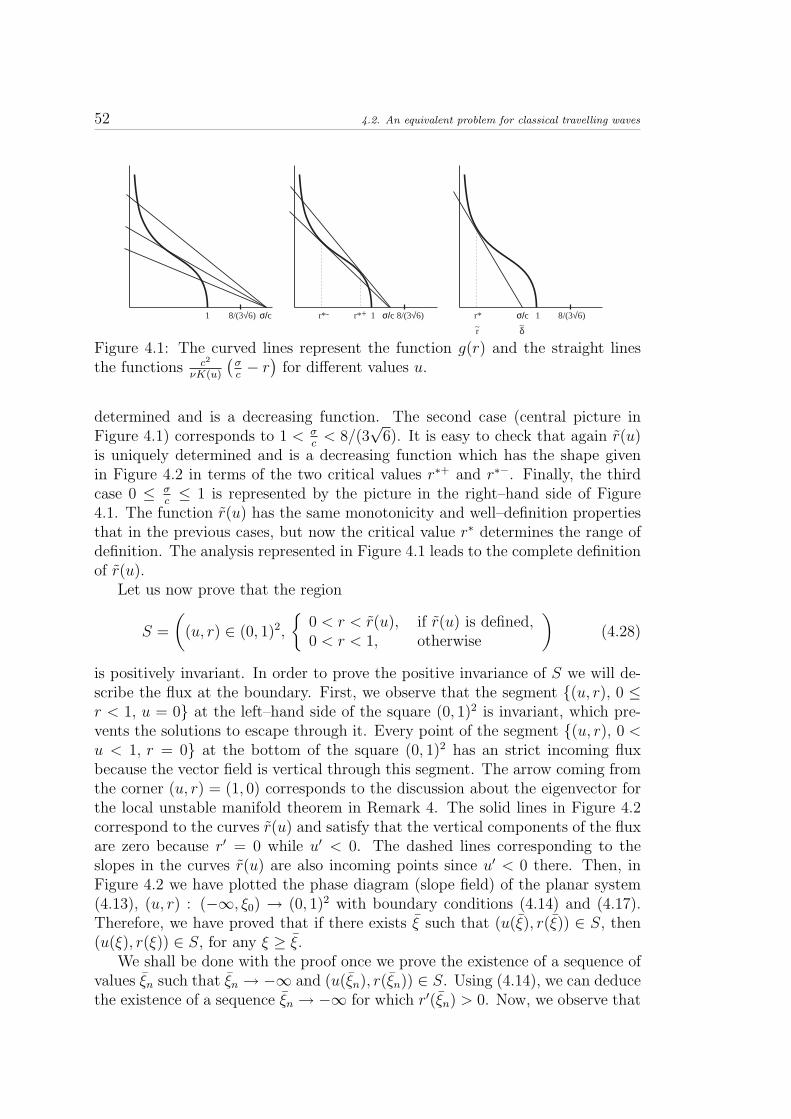
52 4.2. An equivalent problem for classical travelling waves
σ/c1 8/(3√6) σ/c1 8/(3√6)r*+r*- σ/c 1 8/(3√6)r*
r δ~ ~
Figure 4.1: The curved lines represent the function g(r) and the straight linesthe functions c2
νK(u)
(σc− r)
for different values u.
determined and is a decreasing function. The second case (central picture inFigure 4.1) corresponds to 1 < σ
c< 8/(3
√6). It is easy to check that again r(u)
is uniquely determined and is a decreasing function which has the shape givenin Figure 4.2 in terms of the two critical values r∗+ and r∗−. Finally, the thirdcase 0 ≤ σ
c≤ 1 is represented by the picture in the right–hand side of Figure
4.1. The function r(u) has the same monotonicity and well–definition propertiesthat in the previous cases, but now the critical value r∗ determines the range ofdefinition. The analysis represented in Figure 4.1 leads to the complete definitionof r(u).
Let us now prove that the region
S =
((u, r) ∈ (0, 1)2,
0 < r < r(u), if r(u) is defined,0 < r < 1, otherwise
)(4.28)
is positively invariant. In order to prove the positive invariance of S we will de-scribe the flux at the boundary. First, we observe that the segment (u, r), 0 ≤r < 1, u = 0 at the left–hand side of the square (0, 1)2 is invariant, which pre-vents the solutions to escape through it. Every point of the segment (u, r), 0 <u < 1, r = 0 at the bottom of the square (0, 1)2 has an strict incoming fluxbecause the vector field is vertical through this segment. The arrow coming fromthe corner (u, r) = (1, 0) corresponds to the discussion about the eigenvector forthe local unstable manifold theorem in Remark 4. The solid lines in Figure 4.2correspond to the curves r(u) and satisfy that the vertical components of the fluxare zero because r′ = 0 while u′ < 0. The dashed lines corresponding to theslopes in the curves r(u) are also incoming points since u′ < 0 there. Then, inFigure 4.2 we have plotted the phase diagram (slope field) of the planar system(4.13), (u, r) : (−∞, ξ0) → (0, 1)2 with boundary conditions (4.14) and (4.17).Therefore, we have proved that if there exists ξ such that (u(ξ), r(ξ)) ∈ S, then(u(ξ), r(ξ)) ∈ S, for any ξ ≥ ξ.
We shall be done with the proof once we prove the existence of a sequence ofvalues ξn such that ξn → −∞ and (u(ξn), r(ξn)) ∈ S. Using (4.14), we can deducethe existence of a sequence ξn → −∞ for which r′(ξn) > 0. Now, we observe that

4. On the analysis of travelling waves to a nonlinear flux limited reaction–diffusion equation 53
σ/c ≥ 8/(3√6) 1 < σ/c < 8/(3√6)
r*+
r*-
1≥ σ/c ≥ 0
1
r*
1
r(u)~
1 1 1
r(u) r(u)~ ~
r*
1
Figure 4.2: Description of the positive invariant regions S in terms of the curvesr(u).
the graphic of r(u) splits (0, 1)×(0, r∗) into two components characterized by r′ >0 or r′ < 0. Since (u(ξn), r(ξn))→ (1, 0), then (u(ξn), r(ξn)) ∈ S ∩ (0, 1)× (0, r∗)for n large enough.
4.3 Entropy solutions and consequences
In this section we deal with the study of discontinuous traveling waves. So farad authors know, there is no previous literature reporting on the existence ofsingular traveling waves. In this case it is necessary to use the notion of entropysolution for this equation, which has been introduced in [2].
The main result of this section is the following Theorem about existence ofsingular travelling wave solutions.
Theorem 3.7 Assume σ = σ∗ = c. Then, there exists a discontinuous entropytravelling wave solution of (4.2).
The existence of entropy, travelling wave solutions if σ < σ∗ is an open problem.Define
v(t, x) =
u(x− σt), x− σt < ξ0,0, otherwise,
(4.29)
where σ ≤ σ∗ and u : (−∞, ξ0) → (0, 1), ξ0 < ∞, is a solution of (4.8) given byProposition 2.1. (4.16) implies that v is discontinuous.
It is not trivial to prove that some of these functions v are entropy solutions.This follows from the next two results.
Lemma 3.6 Any solution of (4.8) satisfying (4.9)–(4.10) is log-concave in (−∞, ξ0).
Proof. To see that log(v(ξ)) is concave, it is enough to prove that v′(ξ)v(ξ)
is
decreasing. Using the system (4.13) we have
v′(ξ)
v(ξ)= − c
ν
r(ξ)√1− r(ξ)2
.

54 4.3. Entropy solutions and consequences
The result follows from Lemma 2.4, since the function r → r√1−r2 , r ∈ (0, 1), is
strictly increasing.
The following Proposition characterizes the entropy solutions. The proof fol-lows the same lines of Proposition 6.6 in [3], where a similar result was obtainedin the case of compact support solutions for the equation without the reactionFKPP term. Thus, combining Theorem 3.4 and Proposition 6.6 in [3] togetherwith the null flux at infinity for non–compact support solutions and Proposition3.15 in [2] we have
Proposition 3.3 Let v : [0, T ) × R → [0, 1) and Ω = supp(v(0, ·)) be such thatfor any t ∈ [0, T ):
(i) supp(v(t, ·)) = Ωt, where Ωt = Ω +B(0, c t).
(ii) v ∈ C2(Ωt) and satisfies the differential equation (4.2).
(iii) v(t, x) has a vertical contact angle at the boundary of Ωt, for any t ∈ (0, T ).
(iv) v(t, x) is log-concave in Ωt.
Then, v is an entropy solution.
This result allows to select an entropy solution v from those defined by (4.29).Properties (ii) and (iv) of Proposition 3.3 are satisfied by any v, but only whenσ = σ∗ = c the statement (i) holds, i.e. supp(v) = Ω(t). Moreover, we concludethe proof of Theorem 3.7 by proving that, in this case, v has a vertical contactangle at the boundary of Ω(t), and therefore (iii) is also satisfied.
The following result can be deduced directly from Proposition 2.1. We givehere a more explicit behavior of the vertical angle near ξ0.
Lemma 3.7 Let u be a discontinuous travelling wave for σ = σ∗ = c. Then, thevertical angle near ξ0 is of order (ξ0 − ξ)−
12 .
Proof. Our starting point is system (4.13). By using Lemma 2.5 we can assure,when σ ≤ σ∗, that there exists a constant ασ > 0 and ξ0 such that u(ξ0) = ασand r(ξ0) = 1 . In the case σ = σ∗ = c, (4.13) leads to
r′ =1
cK(u)− c
νr
√1− r√1 + r
.
Clearly r′(ξ0) = 1cK(ασ) < ∞. An expansion of r(ξ) in Taylor series around ξ0
allows to find r(ξ) = 1 + 1cK(ασ)(ξ − ξ0) + O((ξ − ξ0)2). Now, combining this
expression with the equation for u and integrating between ξ0 y ξ, 0 < ξ0−ξ 1,we obtain
−log(u(ξ0)) + log(u(ξ)) =c
ν
2(21cK(ασ)
) 12
(ξ0 − ξ)12 − c
ν
(K(ασ)
2c
)(ξ0 − ξ)
32 .

4. On the analysis of travelling waves to a nonlinear flux limited reaction–diffusion equation 55
Neglecting higher–order terms we find u(ξ) = ασe
2
(2 1cK(ασ))
12
(ξ0−ξ)12
or
u(ξ) = ασ + ασ2(
21cK(ασ)
) 12
(ξ0 − ξ)12 , for 0 < ξ0 − ξ 1 ,
after Taylor expansion.
Remark 5 Since classical solutions are in particular entropy solutions, the ex-istence of travelling waves for σ ≥ σ∗ is completed. The existence of an entropysolution for σ < σ∗ is an open question, we can only assure that the correspondingfunction v, defined by (4.29), is not an entropy solution. This follows from thefact established in Theorem 3.9 of [2], that the support of any log-concave solutionmoves with speed c while the support of v(t, ·) moves with σ < c.
Remark 6 The existence of travelling waves having different profiles from wavefronts is also an open question. It can be proved that no more classical (C2) wavefronts exist. The authors conjecture that no more entropy travelling wave solutionwill exist, but it is likely to be a much harder problem.
To conclude this section we propose an application of the travelling wavesolutions with σ∗ < c that allows to bound entropy solutions.
Proposition 3.4 Let u0 : R → [0, 1) be a measurable function with compactsupport and ess sup(u0) < 1. Let u(t, x) be an entropy solution of (4.2) withinitial data u0. Then,
ess supx∈R(u(t, x)) < 1
and for any c > σ > σ∗ there exist positive constants α and β not depending onσ such that
ess sup|x|>σtu(t, x) ≤ αe−β(σ−σ∗)t.
In addition, if σ > c we have
ess sup|x|>σtu(t, x) = 0
for large t.
Proof. Let v∗(t, x) = u∗(x − σ∗t) be a C2 travelling wave solution of (4.2)defined by Theorem 1.6. Then, we can take a translation of u∗, still denotedu∗ for simplicity, such that u∗(ξ) ≥ u0(ξ). A comparison principle for entropysolutions, see Theorem 3.8 in [2], leads to
u(t, x) ≤ u∗(x− σ∗t), a.e. (t, x) ∈ R2.
On the other hand, for a classical travelling wave there exist positive constantsα and β such that
u(ξ) ≤ αe−βξ , ξ ∈ R .

56 4.3. Entropy solutions and consequences
This upper estimate is a consequence of the fact that u∗ is uniformly boundedand limξ→∞
(u∗(ξ))′
u(ξ)is strictly negative as pointed out in (4.18). Hence, we find
u(t, x) ≤ u∗(x− σ∗t) ≤ αe−β(x−σ∗t), a.e. (t, x) ∈ R2. (4.30)
Assuming now that x > σ t, we deduce from (4.30) the inequality
u(t, x) ≤ αe−β(σ−σ∗)t, a.e. (t, x) ∈ R2, x > σ t. (4.31)
In the case x < −σ t we can argue in a similar way by using a classical travellingwave u∗(σ∗t− x) such that u0(ξ) < u∗(−ξ).
The second assertion follows by a comparison argument with the singulartravelling wave defined by (4.29).

Bibliography
[1] Andreu,F., Calvo, J., Mazon, J.M., Soler, J. On a nonlinear flux–limitedequation arising in the transport of morphogens, preprint.
[2] Andreu, F., Caselles, V., Mazon, J.M. A Fisher-Kolmogorov equation withfinite speed of propagation, Journal Dif. Eq 2010, 2528-2561 .
[3] Andreu, F., Caselles, V., Mazon, J.M. Some regularity results on the rela-tivistic heat equation, J. Diff. Equat. 2008, 245, 3639–3663.
[4] Andreu, F., Caselles, V., Mazon, J.M. The Cauchy Problem for a StrongyDegenerate Quasilinear Equation, J. Europ. Math. Soc. 205, 7, 361–393.
[5] Andreu, F., Caselles, V., Mazon, J.M., Moll, S. Finite Propagation Speed forLimited Flux Diffusion Equations, Arch. Ration. Mech. Anal., 2006, 182,269–297.
[6] Apte, S.V., Mahesh, K., Lundgren, T. Accounting for finite-size effects insimulations of disperse particle-laden flows, International Journal of Multi-phase Flow 2008 34, 260271.
[7] Arnold, A., Dhamo, E., Mancini, C. Dispersive effects in quantum kineticequations, to appear in Indiana Univ. Math. J., 2006.
[8] Arnold, A., Lopez, J. L., Markowich, P. A., Soler, J. An analysis of quantumFokker–Planck models: a Wigner function approach, Rev. Mat. Iberoameri-cana 2004, 20, 771–814.
[9] Aronson, D.G., Weinberger,H.F. Nonlinear diffusion in population genet-ics, combustion and nerve propagation, Partial Differential Equations andRelated Topics, Lectures Notes in Math. 1975, Springer, New York, 446,5–49.
[10] Aronson, D.G., Weinberger,H.F. Multidimensional nonlinear diffusions aris-ing in population genetics, Adv. Math. 1978, 30, 33–76.
[11] Auberson, G., Sabatier, P. C. On a class of homogeneous nonlinearSchrodinger equations, J. Math. Phys. 1994, 35(8), 4028–4040.
57

58 BIBLIOGRAPHY
[12] Aubin, J.P. Un theoreme de compacite, C. R. Acad. Sci., Ser, 1963 I 256,5042–5044.
[13] Bellomo, N. Modelling Complex Living Systems. A Kinetic Theory andStochastic Game Approach,Birkhauser-Springer, Boston, 2008.
[14] Berestycki, H., Hamel, F., Nadirashvili, N. The speed of propagation forKPP type problems. I - Periodic framework, J. European Math. Soc., 2007,7,173–213.
[15] Berestycki,H., Rossi, L.Reaction-diffusion equations for population dynamicswith forced speed, I - The case of the whole space, Discrete and ContinousDynamical Systems, 2008, 21, 41–67.
[16] Berestycki, H., Hamel, F. Front propagation in periodic excitable media,Comm. Pure Appl. Math., 2002, 55, 949–1032.
[17] Berestycki, H., Hamel, F. Generalized travelling waves for reaction-diffusionequations, in Perspectives in Nonlinear Partial Differential Equations, Inhonor of H. Brezis, Contemp. Mathematics, 2007, 446, Amer. Math. Soc.,Providence, RI.
[18] Berthelin, F. , Degond, P., Delitala, M., Rascle, M. A model for the formationand evolution of traffic jams, Arch. Rat. Mech. Anal., 2008, 187, 185220.
[19] Brenier, Y. Extended Monge-Kantorovich Theory. Optimal Transportationand Applications: Lectures given at the C.I.M.E. Summer School held inMartina Franca, Italy September 2–8, 2001. Lecture notes in Mathematics,Volume1813 2003, Springer–Verlag, Berlin, 91–122.
[20] Bialynicki–Birula, I., Mycielski, J. Nonlinear wave mechanics, Ann. Phys.1976, 100, 62–93.
[21] Burges, P.K., Kulesa, P.M., Murray, J.D., Alvord E.C. The interaction ofgrowth rates and diffusion coefficients in a three-dimensional mathematicalmodel of gliomas, J Neuropathol Exp Neurol. 1997, 56, 704–13.
[22] Caldeira, A. O., Legget, A. J. Path integral approach to quantum Brownianmotion, Phys. A 1983, 121, 587–616.
[23] Campos J., Guerrero P., Snchez O., Soler J., On the analysis of travellingwaves to a nonlinear flux limited reaction-diffusion equation, Submitted.
[24] Campos D., Fort J,. Llebot, J.E. Reaction-diffusion wave fronts: Multigen-eration biological species under climate change, Phys. Rev. E, 2002, 66,062901.

BIBLIOGRAPHY 59
[25] Canizo, J. A., Lopez, J. L., Nieto, J. Global L1 theory and regularity of the3D nonlinear Wigner–Poisson–Fokker–Planck system, J. Diff. Equ. 2004,198, 356–373.
[26] Castella, F., L2 Solutions to the Schrodinger-Poisson System: Existence,Uniqueness, Time Behaviour, and Smoothing Effects, Math. Mod. Meth. inAppl. Sci., 1997, 8, 1051-1083.
[27] Cazenave, T. An introduction to nonlinear Schrodinger equations,Textos de Metodos Matematicos 22, Rıo de Janeiro, 1989.
[28] Cazenave, T. Stable solutions of the logarithmic Schrodinger equation, Non-linear Analysis T. M. A. 1983, 7(10), 1127–1140.
[29] Cazenave, T., Haraux, A. Equations d’evolution avec non linearite logarith-mique, Annals Fac. Sci. Univ. Toulouse 1980, 2, 21–55.
[30] Cid, C., Dolbeault, J. Defocusing nonlinear Schrodinger equation: confine-ment, stability and asymptotic stability, 2001 (preliminary version).
[31] Constantin, P., Kiselev, A., Oberman, A., Ryzhik, L. Bulk burning rate inpassive-reactive diffusion, Arch. Ration. Mech. Anal., 2000, 154, 53–91.
[32] Cufaro Petroni, N., De Martino, S., De Siena, S., Illuminati, F. Stochastic–hydrodynamic model of halo formation in charged particle beams, Phys. Rev.ST Accel. Beams 2003, 6, 034206.
[33] Czopnik, R., Garbaczewski, P. Quantum potential and random phase–spacedynamics, Phys. Lett. A 2002, 299, 447–453.
[34] Davidson, M. P. A model for the stochastic origins of Schrodinger’s equation,J. Math. Phys. 1979, 20, 1865–1869.
[35] Davidson, M. P. Comments on the nonlinear Schrodinger equation, Il NuovoCimento B 2001, V116B, 1291–1296.
[36] Davis, E. B. Quantum theory of open systems (Academic, London, 1976).
[37] De Martino, S., Falanga, M., Godano, C., Lauro, G. LogarithmicSchrodinger–like equation as a model for magma transport, Europhys. Lett.2003, 63(3), 472–475.
[38] De Martino, S., Lauro, G. Soliton–like solutions for a capillary fluid, Wavesand Stability in Continuous Media, Proceedings of the 12th Conference onWASCOM 2003.
[39] Dekker, H., Valsakumar, M. C. A fundamental constraint on quantum me-chanical diffusion coefficients, Phys. Lett. 1984, 104A(2), 67–71.

60 BIBLIOGRAPHY
[40] Diosi, L. Caldeira–Leggett master equation and medium temperatures., Phys.A 1993, 22, 517–526.
[41] Diosi, L. On high–temperature Markovian equation for quantum Brownianmotion, Europhys. Lett. 1993, 22, 1–3.
[42] Doebner, H. D., Goldin, G. A. On a general nonlinear Schrodinger equationadmitting diffusion currents, Phys. Lett. A 1992, 162, 397–401.
[43] Doebner, H. D., Goldin, G. A., Nattermann, P. A family of nonlinearSchrodinger equations: linearizing transformations and resulting structure,in Quantization, Coherent States and Complex Structures, J.–P. Antoine etal. (Eds.), 27–31, Plenum 1996.
[44] Dolbeault, J., Sanchez, O., Soler, J. Asymptotic behaviour for the Vlasov-Poisson system in the stellar dynamics case., Arch. Ration. Mech. Anal.,2004, 171, 301–327.
[45] Evans, L. C. Partial differential equations, Graduate Studies in Mathe-matics 19, American Mathematical Society, Providence, Rhode Island, 1998.
[46] Fenyes, I. Eine wahrscheinlichkeitstheoretische begrundung und interpreta-tion der Quantenmechanik, Z. Phys. 1952, 132, 81–103.
[47] Fife, P.C. Mathematical aspects of reacting and diffusing systems, LectureNotes in Biomathematics 1979, Springer Verlag, 28.
[48] Fisher, R.A. The advance of advantageous genes, Ann. Eugenics 1937, 7,335–369.
[49] Gao, S. Dissipative quantum dynamics with a Lindblad functional, Phys.Rev. Lett. 1997, 79(17), 3101–3104.
[50] Garbaczewski, P. Modular Schrodinger equation and dynamical duality,Phys. Rev. E 2008, 78, 031101.
[51] Gardner, C., The quantum hydrodynamic model for semiconductor devices,SIAM J. Appl. Math., 1994 54, 409–427.
[52] J. Ginibre and G. Velo, On a class of nonlinear Schrodinger equations I andII, J. Funct. Anal., 32(1), (1979), 1–32 and 33–71.
[53] Goldin, G., Shtelen, V. On gauge transformations of Backlund type andhigher order nonlinear Schrodinger equations, J. Math. Phys. 2002, 43(5),2180–2186.
[54] Grant, Christopher P. Theory of Ordinary Differential Equations, BrighamYoung University.

BIBLIOGRAPHY 61
[55] Grossmann, F., Koch, W. A finite–difference implementation of theCaldeira–Leggett master equation, J. Chem. Phys. 2009, 130(3), 034105.
[56] Guerra, F. Structural aspects of stochastic mechanics and stochastic fieldtheory, Phys. Rep. 1981, 77(3), 263–312.
[57] Guerra, F., Pusterla, M. A nonlinear Schrodinger equation and its relativisticgeneralization from basic principles, Lett. Nuovo Cimento 1982, 34, 351–356.
[58] Guerrero, P., Lopez, J. L., Nieto, J. Global H1 solvability of the 3D loga-rithmic Schrodinger equation, Nonlinear Analysis: Real World Applications2010, 11, 79–87.
[59] Guerrero, P., Lopez, J. L., Montejo–Gamez, J., Nieto, J. Wellposednessof a nonlinear Schrodinger equation of logarithmic type modeling quantumdissipation, work in progress.
[60] Guerrero, P., Lopez, J. L., Montejo–Gamez, J., Nieto, J. A wavefunctiondescription of stochastic–mechanical Fokker–Planck dissipation: derivation,stationary dynamics and numerical approximation, preprint.
[61] Hadeler,K.P. , Rothe, F. Travelling fronts in nonlinear diffusion equations,J. Math. Biol. 1975 2, 251–263.
[62] Hartman, P. Ordinary Differential Equations, Wiley, New York, 1964.
[63] Hefter, E.F. Application of the nonlinear Schrodinger equation with a log-arithmic inhomegeneous term to nuclear physics, Phys. Rev. A, 1985 32,1201–1204.
[64] Jungel, A., Mariani, M. C., Rial, D. Local existence of solutions to thetransient quantum hydrodynamic equations, Math. Models Meth. Appl. Sci.2002, 12(4), 485–495.
[65] Kolmogorov, A.N., Petrovsky, I.G., Piskunov, N.S. Etude de lequation de ladiffusion avec croissance de la quantite de matiere et son application a unproblme biologique, Bulletin Universite dEtata Moscou (Bjul. MoskowskogoGos. Univ.), Serie internationale A 1 1937, 1-26. See English translation in:Dynamics of curved fronts, P. Pelce Ed., Academic Press, 1988, 105–130.
[66] Kostin, M. D. On the Schrodinger–Langevin equation. J. Chem. Phys. 1972,57, 3589–3591.
[67] Lauro, G. A note on a Korteweg fluid and the hydrodynamic form of thelogarithmic Schrodinger equation, Geophys. and Astrophys. Fluid Dynamics2008, 102(4), 373–380.
62 BIBLIOGRAPHY
[68] Lemos, N.A. Dissipative forces and the algebra of operators in stochasticquantum mechanics, Phys. Lett. A, 1980 78, 239–241.
[69] Lindblad, G. On the generators of quantum dynamical semigroups, Comm.Math. Phys. 1976, 48, 119–130.
[70] Lopez, J. L. Nonlinear Ginzburg–Landau–type approach to quantum dissipa-tion, Phys. Rev. E. 2004, 69, 026110.
[71] Lopez, J. L., Montejo–Gamez, J. A hydrodynamic approach to multidimen-sional dissipation-based Schrodinger models from quantum Fokker-Planckdynamics, Physica D 2009, 238(6), 622–644.
[72] Lopez, J. L., Nieto, J. Global solutions of the mean–field, very high tem-perature Caldeira–Leggett master equation. Quart. Appl. Math. 2006, 64,189–199.
[73] Lopez, J.L., Soler, J. Asymptotic behaviour to the 3–D Schrodinger/Hartree–Poisson and Wigner–Poisson systems, Math. Mod. Meth. Appl. Sci., 200010(6), 923–943.
[74] Majda, A.J., Souganidis, P.E.Flame fronts in a turbulent combustion modelwith fractal velocity fields, Comm. Pure Appl. Math. 1998, 51, 1337–1348.
[75] Madelung, E. Quantentheorie in hydrodynamischer form, Z. Phys. 1927,40, 322–326.
[76] Meinhardt, H. Models of Biological Pattern Formation, Academic Press,1982.
[77] Mihalas, D., Mihalas, B. Foundations of Radiation Hydrodynamics, OxfordUniversity Press, Oxford, 1984.
[78] Murray, J. D. Mathematical Biology, Springer-Verlag, 1996.
[79] Nassar, A.B. New method for the solution of the logarithmic nonlinearSchrodinger equation via stochastic mechanics, Phys. Rev. A, 1985 33,3502–3505.
[80] Nattermann, P., Scherer, W. Nonlinear gauge transformations and exactsolutions of the Doebner–Goldin equation, in Nonlinear, Deformed and Irre-versible Quantum Systems, Doebner et al. (Eds.), 188–199, World Scientific1995.
[81] Nelson, E. Derivation of the Schrodinger equation from Newtonian Mechan-ics, Phys. Rev. 1966, 150, 1079–1085.
[82] Nieto, J., Poupaud, F., Soler, J. High–field limit for the Vlasov–Poisson–Fokker–Planck system, Archive Rat. Mech. Anal. 2001, 158(1), 29–59.

BIBLIOGRAPHY 63
[83] Pazy A., Semigroups of Linear Operators and Applications toPartial Differential Equations, Applied Mathematical Sciences,Vol. 44(Springer-Verlag, 1983).
[84] Pollak, E., Zhang, S. Quantum dynamics for dissipative systems: A nu-merical study of the Wigner–Fokker–Planck equation, J. Chem. Phys. 2003,118(10), 4357–4364.
[85] Ramazanoglu, F. The approach to thermal equilibrium in the Caldeira–Leggett model, J. Phys. A: Mathematical and Theorical 2009, 42(26), 265303.
[86] Ringhofer, C., Soler, J. Discrete Schrodinger–Poisson systems preservingenergy and mass, Appl. Math. Lett. 2000, 13(7), 27–32.
[87] Rinzel, J., Keller, J.B. Traveling wave solutions of a nerve conduction equa-tion, Biophysical Journal 1973, 13, 1313-1336.
[88] Rosenau, Ph. Tempered Diffusion: A Transport Process with PropagatingFront and Inertial Delay, Phys. Review A, 1992, 46, 7371-7374.
[89] Sabatier, P.C. Multidimensional nonlinear Schrodinger equations with expo-nentially confined solutions, Inverse Problems, 1990 6, L47–L53.
[90] Saha, K., Schaffer, D.V. Signal dynamics in Sonic hedgehog tissue patterning,Development 2006,133, 889-900.
[91] Sanchez-Garduno, F., Maini, P. K. Existence and uniqueness of a sharptravelling wave in degenerate non-linear diffusion Fisher-KPP equations, J.Math. Biol. 1994, 33, 163-192.
[92] Sattinger, D.H.Stability of waves of nonlinear parabolic systems, Adv. Math.1976, 22, 312–355.
[93] Shigesada, N., Kawasaki, K. Biological Invansion: Theory and Prac-tice, Oxford Press, 1997.
[94] Turing, A. M. The chemical basis of morphogenesis, Philosoph. Trans. RoyalSoc . London, vol. 1952 237(B), 37–72.
[95] Vacchini, B. Completely positive quantum dissipation, Phys. Rev. Lett. 2000,84(7), 1374–1377.
[96] Volpert, A.I., Volpert, V.A., Volpert, V.A. Travelling wave solutions ofparabolic systems], Translations of Math. Monographs 1994, Amer. Math.Soc., 140.
[97] Wallstrom, T. C. Ineqiuvalence between the Schrodinger equation and theMadelung hydrodynamic equations, Phys. Rev. A 1994, 49(3), 1613–1617.