![Ocala Evening Star. (Ocala, Florida) 1904-09-24 [p Page [Two]]. - UFDC Image Array 2ufdcimages.uflib.ufl.edu/UF/00/07/59/08/01701/00305.pdf · 2009. 5. 13. · Bail CAPITAL FAST JEWELER](https://static.fdocuments.in/doc/165x107/60d02a4254a96f353010cadc/ocala-evening-star-ocala-florida-1904-09-24-p-page-two-ufdc-image-array.jpg)
anagnostis_g ( PDF ) - UFDC Image Array 2 - University of Florida
105
DESIGN POINT ANALYSIS OF THE HIGH PRESSURE REGENERATIVE TURBINE ENGINE CYCLE FOR HIGH-SPEED MARINE APPLICATIONS By GEORGE ANAGNOSTIS A THESIS PRESENTED TO THE GRADUATE SCHOOL OF THE UNIVERSITY OF FLORIDA IN PARTIAL FULFILLMENT OF THE REQUIREMENTS FOR THE DEGREE OF MASTER OF SCIENCE UNIVERSITY OF FLORIDA 2007
Transcript of anagnostis_g ( PDF ) - UFDC Image Array 2 - University of Florida

DESIGN POINT ANALYSIS OF THE HIGH PRESSURE REGENERATIVE TURBINE ENGINE CYCLE FOR HIGH-SPEED MARINE APPLICATIONS
By
GEORGE ANAGNOSTIS
A THESIS PRESENTED TO THE GRADUATE SCHOOL OF THE UNIVERSITY OF FLORIDA IN PARTIAL FULFILLMENT
OF THE REQUIREMENTS FOR THE DEGREE OF MASTER OF SCIENCE
UNIVERSITY OF FLORIDA
2007

Copyright 2007
By
George Anagnostis

This thesis is dedicated to my parents, Victor and Linda Anagnostis. Without their emotional and financial encouragement this thesis would not exist.

iv
ACKNOWLEDGMENTS
I thank the members of my graduate committee members: Dr. William E. Lear, Jr.,
Dr. S. A. Sherif, and Dr. Herbert Ingley for their support on this thesis. Dr. Lear was
especially helpful, providing me with critical advice throughout this project. Next, I
would like to thank the Aeropropulsion Systems Analysis Office at the National
Aeronautics and Space Administration Glenn Research Center for their assistance on
Numerical Propulsion System Simulation program. Two members of that group provided
continued technical assistance—Scott Jones and Thomas Lavelle. Lastly, I thank two
special individuals that have provided me with insight and wisdom concerning matters of
engineering and life in general, John Crittenden and William Ellis.

v
TABLE OF CONTENTS page
ACKNOWLEDGMENTS ................................................................................................. iv
LIST OF TABLES............................................................................................................ vii
LIST OF FIGURES ......................................................................................................... viii
NOMENCLATURE ............................................................................................................x
CHAPTER
1 INTRODUCTION ........................................................................................................1
2 LITERATURE REVIEW .............................................................................................4
Brief History of Turbine Engine Development ............................................................4 Gas Turbine Engine Examples in Marine Applications ...............................................5 Advantages of Gas Turbine Engines in Marine Applications ......................................6 Recuperation and Inter-cooling ....................................................................................7 Semi-Closed Cycles......................................................................................................9 Computer Code Simulators.........................................................................................10 Previous Gas Turbine Research at the University of Florida .....................................12
3 NUMERICAL PROPULSION SYSTEM SIMULATION ARCHITECTURE.........16
Model..........................................................................................................................16 Elements .....................................................................................................................17 FlowStation.................................................................................................................18 FlowStartEnd ..............................................................................................................18 Thermodynamic Properties Package ..........................................................................20 Solver..........................................................................................................................21
4 CYCLE CONFIGURATIONS AND BASE POINT ASSUMPTIONS.....................25
Major Model Features.................................................................................................25 Flow Path Descriptions & Schematics .......................................................................26
Simple Cycle Gas Turbine Engine Model...........................................................26 High Pressure Regenerative Turbine Engine Efficiency Model .........................26

vi
High Pressure Regenerative Turbine Engine with Vapor Absorption Refrigeration System Efficiency Model ..........................................................27
Simple Cycle Gas Turbine Engine Design Assumptions and HPRTE Cycles Base Point Assumptions .................................................................................................28
5 THERMODYNAMIC MODELING AND ANALYSIS............................................33
Thermodynamic Elements ..........................................................................................33 Heat Exchangers..................................................................................................33 Mixers..................................................................................................................34 Splitter .................................................................................................................35 Water Extractor ...................................................................................................36 Compressors ........................................................................................................37 Turbines...............................................................................................................39 Burner ..................................................................................................................40
Sensitivity Analysis ....................................................................................................41
6 RESULTS AND DISCUSSION.................................................................................43
Cycle Code Comparison .............................................................................................43 Sensitivity Analysis ....................................................................................................44
Simple Cycle Gas Turbine Engine Model...........................................................44 Simple Cycle Gas Turbine Engine Model Sensitivity Analysis..........................48 High Pressure Regenerative Turbine Engine Efficiency Model .........................50 High Pressure Regenerative Turbine Engine Efficiency Model Sensitivity
Analysis............................................................................................................53 Cycle Comparison Analysis .......................................................................................61
Extreme Operating Conditions ............................................................................65 High Pressure Compressor Inlet Temperature Comparison for H-V Efficiency
Model ...............................................................................................................67 Final Design Point Parameter Comparison .........................................................68
7 CONCLUSIONS AND RECOMMENDATIONS.....................................................83
Conclusions.................................................................................................................83 Recommendations.......................................................................................................86
LIST OF REFERENCES...................................................................................................88
BIOGRAPHICAL SKETCH .............................................................................................91

vii
LIST OF TABLES
Table page 4-1 Comparison of major configuration features ...........................................................29
4-2 Simple Cycle Gas Turbine engine design point parameters.....................................32
4-3 Base case model assumptions for HPRTE cycles [3], [26], [27] .............................32
6-1 Cycle codes comparison: NPSS verses spreadsheet code for HPRTE Efficiency model data run. All temperatures are in °R. ............................................................70
6-2 Summary of the HPRTE Efficiency sensitivity analysis .........................................77
6-3 Comparison of the thermal efficiency maximums and their corresponding overall pressure ratios (OPRs)..................................................................................78
6-4 Comparison of the specific power maximum values and their corresponding OPRs.........................................................................................................................78
6-5 Comparison of exhaust temperature maximum values for the three engine configurations...........................................................................................................79
6-6 Engine cycles comparison for four extreme operating conditions ...........................81
6-7 High pressure compressor (HPC) inlet temperature comparison for the H-V Efficiency engine model...........................................................................................81
6-8 Final performance design point comparison for the engine configurations.............82

viii
LIST OF FIGURES
Figure page 3-1 Example NPSS engine model [19]...........................................................................23
3-2 State 7 of HPRTE engine cycle................................................................................24
4-1 Simple Cycle Gas Turbine (SCGT) engine model configuration ............................29
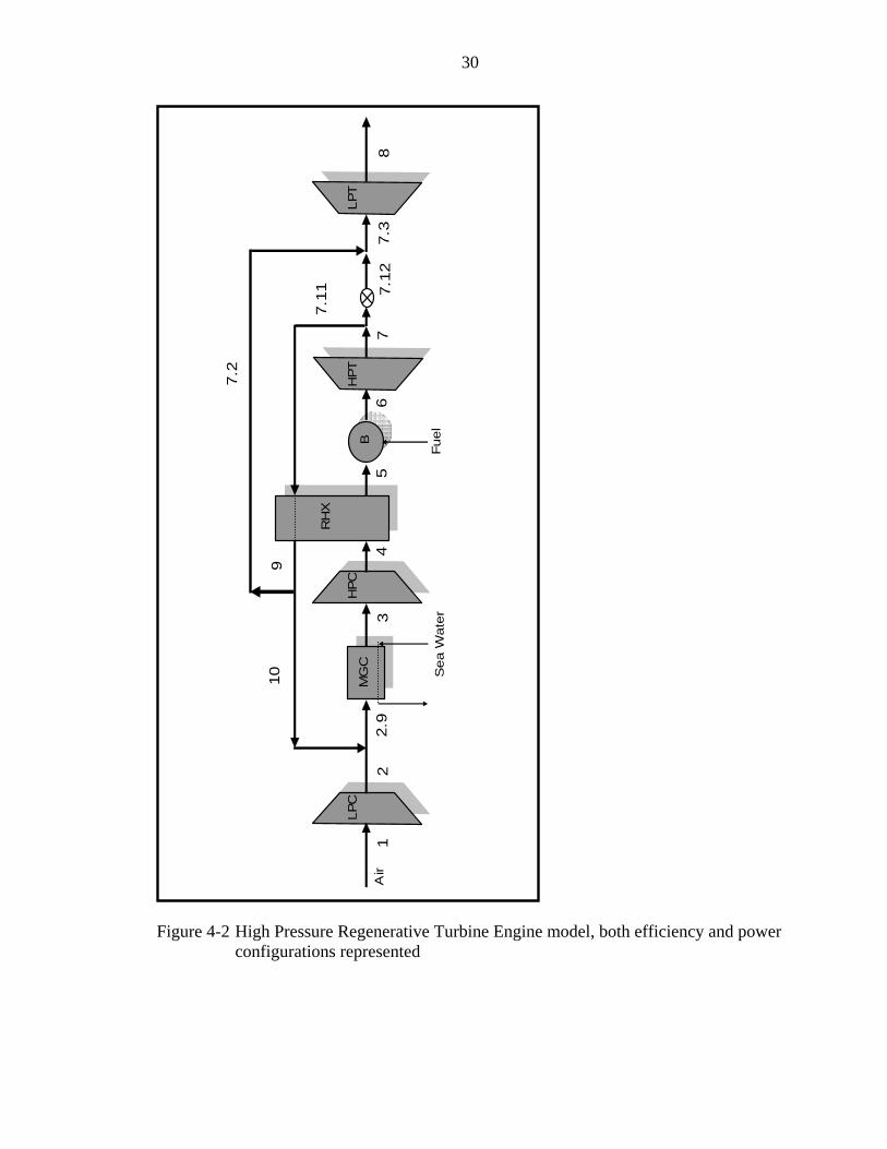
4-2 High Pressure Regenerative Turbine Engine model, both efficiency and power configurations represented .......................................................................................30
4-3 High Pressure Regenerative Turbine Engine-Vapor Absorption Refrigeration System, both efficiency and power model configurations represented....................31
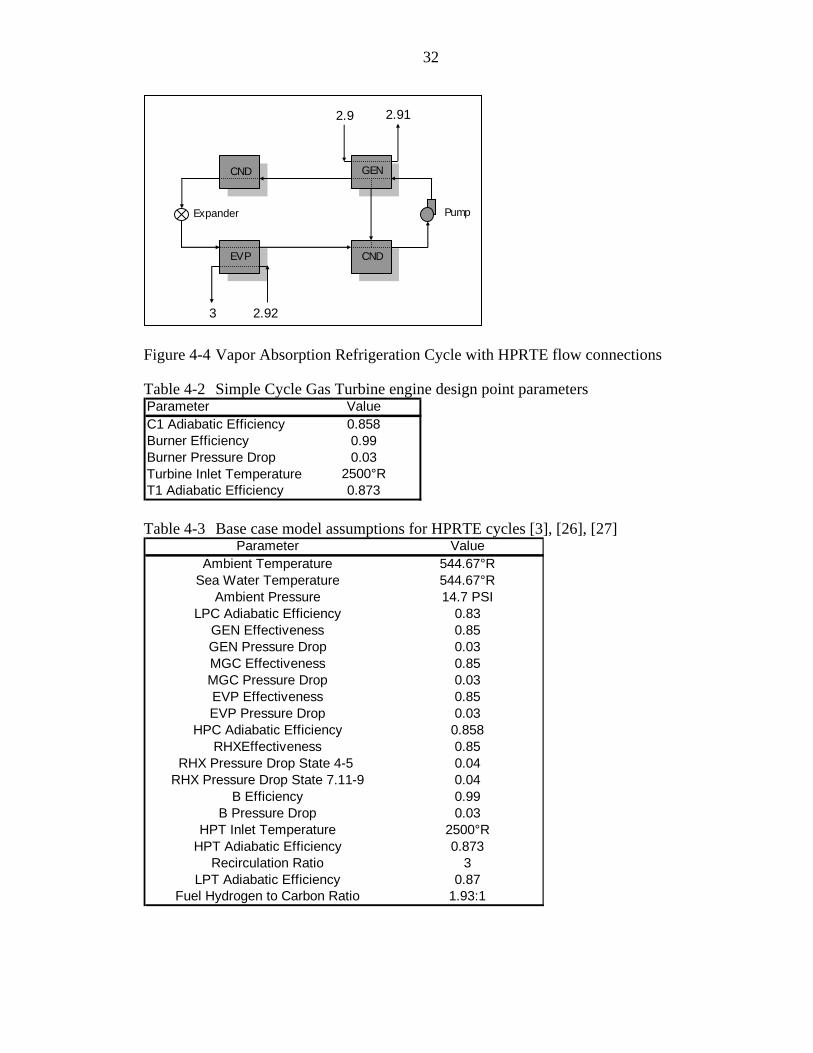
4-4 Vapor Absorption Refrigeration Cycle with HPRTE flow connections ..................32
6-1 Thermal efficiency comparison is plotted with respect to OPR. NPSS results (with turbine inlet temperature (TIT) set to 2500°R) are compared to the derived and the ideal Brayton cycle expressions. .................................................................70
6-2 Thermal efficiency vs. OPR with sensitivity to TIT ................................................71
6-3 Specific power vs. OPR with TIT sensitivity...........................................................71
6-4 Thermal efficiency vs. ambient temperature with OPR sensitivity..........................72
6-5 Demonstrates agreement between NPSS and developed theory that describes the low pressure spool ....................................................................................................72
6-6 High pressure spool pressure ratio (HPPR) vs. ambient temperature with low pressure spool pressure ratio (LPPR) sensitivity......................................................73
6-7 Thermal efficiency vs. HPPR showing sensitivity to TIT .......................................73
6-8 Thermal efficiency vs. HPC inlet temperature for recirculation ratio sensitivity ....74
6-9 Thermal efficiency vs. turbine exit temperature (TET) with cooler pressure drop sensitivity .................................................................................................................74
6-10 Specific power vs. TET for HPC efficiency sensitivity ...........................................75

ix
6-11 Specific power vs. HPPR for HPT efficiency sensitivity.........................................75
6-12 Exhaust temperature vs. OPR for TIT sensitivity ....................................................76
6-13 Thermal efficiency vs. HPPR for turbocharger efficiency sensitivity .....................76
6-14 Thermal efficiency vs. LPPR for TIT sensitivity .....................................................77
6-15 Engine cycles comparison of thermal efficiency vs. OPR .......................................78
6-16 Engine cycles comparison of specific power vs. OPR.............................................79
6-17 Engine cycles comparison of exhaust temperature vs. OPR....................................80
6-18 Engine cycles comparison of thermal efficiency vs. ambient temperature..............80

x
NOMENCLATURE
DepV Dependent variable in a Jacobian matrix
IndV Independent variable in a Jacobian matrix
ε Heat exchanger effectiveness
inPP _0Δ Pressure drop as a percentage of the inlet stream pressure
Q& Heat flow rate (Btu/sec)
nm& Mass flow rate at station “n” (lbm/sec)
npC _ Specific heat at constant pressure at flow station “n” (Btu/lbm-°R)
inT _0 Stagnation temperature at the inlet to a physical cycle component (°R)
outT _0 Stagnation temperature at the exit to a physical cycle component (°R)
inP _0 Stagnation pressure at the inlet to a physical cycle component (psi)
outP _0 Stagnation pressure at the exit to a physical cycle component (psi)
inh _0 Mass specific stagnation enthalpy at the inlet to a physical cycle
component (Btu/sec-lbm)
outh _0 Mass specific stagnation enthalpy at the inlet to a physical cycle
component (Btu/sec-lbm)
nFAR Fuel-to-air ratio at state point “n”

xi
ntotm _& For splitters and separators, total mass flow rate at state point “n”
(lbm/sec)
BPR Flow bypass ratio for splitter elements
liquidOHm _2& Mass flow rate of liquid water being extracted in separator (lbm/sec)
liquidOHh _2 Mass specific enthalpy of liquid water being extracted (Btu/sec-lbm)
CompPR Pressure ratio any compressor
adComp _η Adiabatic efficiency of any compressor
ns _0 Mass specific stagnation entropy at flow station “n” (Btu/lbm-°R)
R Ideal gas constant (Btu/lbm-°R)
idh Mass specific enthalpy change for an isentropic process (Btu/sec-lbm)
inCompR _ Ideal gas constant at a compressor inlet state point (Btu/lbm-°R)
bη Burner efficiency
RQ Lower heating value of the fuel (Btu/lbm)
WAR Water to air ratio, mass basis
TIT Turbine inlet temperature
OPR Overall pressure ratio of a system
γ Ratio of specific heats, v
p
CC
SpPw Specific Power (HP-sec/lbm)
ambT Ambient Temperature (°R), also ambientT
LPPR Low pressure compressor pressure ratio
HPRR High pressure compressor pressure ratio

xii
adLPC _η Low pressure compressor adiabatic efficiency
adLPT _η Low pressure turbine adiabatic efficiency

xiii
Abstract of Thesis Presented to the Graduate School
of the University of Florida in Partial Fulfillment of the Requirements for the Degree of Master of Science
DESIGN POINT ANALYSIS OF THE HIGH PRESSURE REGENERATIVE TURBINE ENGINE CYCLE FOR HIGH-SPEED MARINE APPLICATIONS
By
George Anagnostis
May 2007
Chair: William E. Lear, Jr. Major Department: Mechanical and Aerospace Engineering
A thermodynamic sensitivity and performance analysis was performed on the High
Pressure Regenerative Turbine Engine (HPRTE) and its combined cycle variation, the
HPRTE with a vapor absorption refrigeration system (VARS). The performance analysis
consisted of a comparison of three engine configurations, the two HPRTE variants and a
simple cycle gas turbine engine (SCGT), modeled after the production marine gas turbine
engine, ETF-40B. The engine cycles were optimized using a parametric analysis; a
sensitivities study was completed to establish which design parameters influence
individual engine model performance. The NASA gas turbine cycle code Numerical
Propulsion System Simulation (NPSS) was the software platform used to complete this
analysis.
The comparison was performed at sea level with an ambient temperature of 544°R.
The results for the SCGT predict a design-point optimized thermal efficiency of 33.4%
and an overall pressure ratio (OPR) of 10.4 with a specific power of 180 HP-sec/lbm.

xiv
The HPRTE engine, called HPRTE Efficiency for this thesis, had an expected design
thermal efficiency of 37.2% (OPR of 32.2) with a specific power rating of 593 HP-
sec/lbm—229% larger than the SCGT specific power. The combined-cycle HPRTE-
VARS, called H-V Efficiency in the analysis, had a predicted design thermal efficiency
of 45.0% (OPR of 32) with a specific power of 629 HP-sec/lbm. The H-V Efficiency
thermal efficiency was 34.7% higher than that of the SCGT designed for maximum
specific power. Exhaust gas temperatures varied significantly between the SCGT and the
HPRTE variants. The model engine exhaust for the SCGT was 1580°R while the exhaust
temperatures of the HPRTE Efficiency and H-V Efficiency were 801°R and 837°R,
respectively. On average, the HPRTE calculated exhaust temperature was 761°R less
than that of the SCGT. High pressure compressor (HPC) inlet temperature sensitivity
was considered for the H-V Efficiency. Two operating cases were considered—the HPC
inlet held constant at 499°R and 509°R. The 499°R case operated with a thermal
efficiency higher by 1.56% and a specific power higher by 1.62%.
The results of the analysis imply that HPRTE duct sizes will be smaller due to the
engine having significantly higher specific power. Since specific fuel consumption is
inversely proportional to thermal efficiency, the H-V Efficiency engine cycle will require
a smaller fuel tank to allow for additional cargo (or if the tank size is unchanged, the ship
range is increased). Future project considerations include an off-design performance
analysis using NPSS or another software package, additional NPSS model benchmarking
with a reputable cycle simulation code, and an analysis of the effects of moist ambient air
on evaporator water flow extraction rates.

1
CHAPTER 1 INTRODUCTION
Before the marine gas turbine, naval ships clipped through the water propelled by
sooty coal-fired steam turbines or diesel engines. The 1940s advent of the gas turbine jet
engine introduced a similar technology shift in the marine propulsion industry a decade
later. And now for the last 60 years marine gas turbine engine propulsion advancements
have derived mainly from aeronautical research and development programs. However,
there have been some instances where the marine propulsion industry has led the way in
development—most notably by the introduction of the Westinghouse-Rolls-Royce 21st
century (WR21) ICR program in the early 1990s. Inter-cooled compressors and exhaust
heat recuperation set the WR21 gas turbine engine apart. Ironically, the same ingenuity
that steered the Navy to develop the WR21 program was nowhere to be found during the
decision-making process time for the propulsion system for the 21st century speed ship-
to-shore transport.
The ETF-40B, a workhorse and variant of the original TF-40 that powered the
Navy landing craft air-cushion (LCAC) vessel for the last two decades will provide the
propulsion and lift thrust for the new J-MAC ship-to-shore transport. Despite interest in
new engine technologies, such as the High Power Regenerative Turbine Engine
(HPRTE), funding constraints prevented the Navy from further investigating novel
systems. This thesis will make the case for the HPRTE as an alternative engine concept
to the ETF-40B for the J-MAC program.

2
The motivation to compare the HPRTE to the ETF-40B is a result of previous
experimental and computational modeling efforts completed at the University of Florida
(UF) Energy and Gas Dynamics Laboratory to develop alternate engine technologies.
There other design considerations besides cost that drive engine development; the
HPRTE will outperform the ETF-40B, having a higher specific power ratio, improved
off-design performance, and a considerably lower infrared heat signature.
The HPRTE is a semi-closed, compressor inter-cooled, recuperative system. A
demonstration engine has been build and performance tested at UF, and the proof of
concept has been met. The laboratory demonstrator uses engine exhaust heat to power a
vapor absorption refrigeration system (VARS). This is representative of the combined
cycle system, one of the two HPRTE configurations, that is considered in this modeling
and analysis project. The base HPRTE is the other. The combined cycle variant is
expected to outperform the base HPRTE because the VARS unit provides additional
cooling to the high pressure compressor inlet of the engine.
The analysis in this thesis includes a parametric optimization and sensitivity studies
that determine design-critical parameters. There are three engine models total that are
considered—the two HPRTE variants (HPRTE Efficiency and H-V Efficiency) and a
simple cycle gas turbine engine (SCGT). The SCGT is modeled to represent the ETF-
40B engine configuration. Only two of the three engines examined are considered in the
sensitivity analysis; they are the SCGT and HPRTE Efficiency engine models. Sensitive
parameters for the HPRTE Efficiency are expected to be the similar for the H-V
Efficiency cycle, and therefore the exercise was deemed redundant.

3
The second part of the project is the cycle comparison analysis which will examine
the performance parameters such as thermal efficiency, specific power, exhaust gas
temperature, and high pressure compressor inlet temperature. Mission specifications and
material and component limitations provide the scope for many of engine variables that
are to be optimized. Being for a military application, the engine is expected to have
robust performance capabilities; therefore, run cases were analyzed representing a wide
range of ambient operating conditions for all cycle configurations.
The model processes were based on thermodynamics relationships. The complete
set of equations used to close the cycle model is discussed later. The flows were all
considered steady-state and incompressible, and the turbomachinery components and
ducting were all represented as adiabatic processes.
These considerations are built in to the cycle code called Numerical Propulsion
System Simulation (NPSS). This is a DOS driven, object-oriented program that has
design, off-design, and transient run operation capabilities. Technical support for this
program was provided by the ASAO group at the NASA Glenn Research Facility.

4
CHAPTER 2 LITERATURE REVIEW
Brief History of Turbine Engine Development
Between 150-50 B.C., a Greek named Hero, living in Alexandria, Egypt, boiled
water in a sealed container that had two spouts extending from the top and slightly curved
[1]. As the water boiled, steam billowed from the spouts, rotating the entire container.
At the time it was considered a toy, but today history remembers Hero as the inventor of
the steam turbine.
Despite this early application, the first documented use of the turbine engine for
propulsion purpose was not until 1791; John Barber, a British inventor designed a simple
steam engine with a chain-driven compressor to power an automobile [1]. Then in 1872,
nearly 100 years after Barber engine, steam-powered automobile was designed, Franz
Stolze designed the first axial gas turbine engine [2]. The practicality of the engine was
suspect and it never ran unassisted.
Interest in gas turbine engines continued to increase, and developmental
breakthroughs were made in the 1930s. Great Britain and Germany were the spearhead
of these efforts as tension between the European heavyweights mounted. Faster, more
agile aircraft were being conceived, and the air forces of both nations noticed the
advantages of the jet engine over conventional piston engines. Frank Whittle of Great
Britain worked out a concept for a turbojet engine and won a patent for it in 1930 [3].
Five years later in Germany Hans van Ohaim, working independently of Whittle,
patented his own gas turbine engine system [3]. Ohaim and his colleagues witnessed the

5
first flight of their turbojet engine on August 27, 1939, powering the He.S3B aircraft [3].
The Whittle concept was shelved until mid 1935 when finally with the help of two ex-
Royal Air Force pilots the engine was built and tested by Power Jets Ltd [3]. After
working through design setbacks, including fuel control issues, the first British—
designed turbojet-powered aircraft flew in May 1941 [3]. Even though the Germans
could claim the first turbojet powered flight, the British built the first production turbojet
engine, the Roll-Royce de Haviland [3]. Turbojet development sky-rocketed in the 1940s
and 1950s; a Whittle design provided the blueprints for the first American made turbojet
engine, the General Electric I-A [7].
Gas Turbine Engine Examples in Marine Applications
The British were using simple gas turbine engines to power gun boats as early as
1947 [4]. The HMS Grey Goose was the first marine vessel to be powered by a
turboshaft engine with an inter-cooled compressor and exhaust heat recuperation (ICR)
[5]. In 1956, the U.S. Navy contracted with Westinghouse to develop a gas turbine
engine for submersible operation [6]. They designed a two shaft semi-closed ICR engine;
a novel concept that but was limited by fuel-type availability. The use of heavy sulfur
fuels triggered sulfuric acid build-up in the intercoolers which degraded the metal
components in the heat exchanger. A direct effect heat exchanger was tried with sea
water, but this only succeeded in introducing salt into the engine which deposited on the
turbomachinery parts [6]. At the same time the Westinghouse engine was under
development, General Electric was looking to convert their profitable J79 engine into a
marine gas turbine. In 1959 they introduced the LM1500. It was a simple cycle gas
turbine that produced 12,500 SHP [7]. The General Electric LM2500, introduced in
1968, ushered in the second generation marine of marine turboshaft engines. Like the

6
LM1500, the LM2500 was a derivate of a proven aero engine that powered over 300 U.S.
Naval ships [8, 7]. Moreover, thermal efficiency was improved on the LM2500 to 37
percent [8].
Advantages of Gas Turbine Engines in Marine Applications
Gas turbine engines have overtaken diesels as the power plant of choice for ferries,
cruise liners and fast-attack military ships. This trend exists because gas turbines offer
higher power output-to-weight ratios, significantly higher compactness, higher
availability, and they produce fewer emissions than marine diesels [9, 4]. The power-to-
weight advantage is best realized with an example comparing a diesel engine to a gas
turbine engine of similar power rating. The 7FDM16 marine diesel offered from General
Electric produces 4100 BHP and weighs 48,800 lbs [10]. In comparison the Lycoming
TF-40 turboshaft marine engine, produces 4,000 BHP and weighs only 1,325 lbs [11].
The significant weight disparity favoring the TF-40 is a prime reason gas turbines are
being chosen to power marine vessels requiring agility and speed. Similarly, the
compactness that gas turbine engines offer greatly improves vessel versatility and crew
and cargo capacity optimization. As an example, the 7FDM16 diesel has a volume of
920 cubic feet, whereas the TF-40 has a volume of less than 43 cubic feet [10, 11].
Subsequently, the compact, light-weight gas turbines are easier to transport and switch-
out of ships. With skilled professionals available from the aviation industry trained on
gas turbines engines, there is an abundance of mechanics and support crew able to
maintain and operate these systems [4]. Moreover, the emission reductions achieved by
gas turbine engines over comparable diesels make them more attractive to commercial
and military forces needing to placate environmental agencies such as the EPA and other

7
international bodies. A simple open-cycle gas turbine engine produces 1/3 to ¼ the
emissions of a diesel engine of comparable technology [9].
Recuperation and Inter-cooling
Simple, open-cycle turbo-shaft engines exhaust hot gas products to the atmosphere
wasting high—quality heat energy; an increasingly common use of this available heat
energy in gas turbine engines is to pre-heat the compressed gas flow before the
combustion stage. This process is called exhaust heat recuperation. As a result of raising
the combustor inlet temperature, less fuel is required to achieve the desired turbine inlet
temperature and desired power output. This directly impacts the thermal efficiency and
specific power of the engine, raising thermal efficiency but dropping specific power in
most cases. Any instance in which fuel use can be decreased has a direct positive impact
on the cycle thermal efficiency. It is important to note that gas turbine engine
recuperators generally work better in engines with only moderate pressure ratios [12].
Qualitatively, one can see that as the engine pressure ratio rises, the compressor exit
temperature and turbine exit temperature approach each other. In practice this would
drop the capacity of the recuperator to pre-heat the compressed air before combustion,
thus rendering it ineffective.
A second improvement on the simple gas turbine engine is the addition of an inter-
cooler. Inter-coolers are placed between the low pressure and high pressure compressors
to reduce the air temperature exiting the last stage of the compressor. Assuming the
process is adiabatic and the air is a calorically perfect gas, the power required to drive the
compressor is written as TcmW pcomp Δ= && . This assumes a control volume analysis
around the entire compressor for all stages [3]. The inter-cooler delivers a lower

8
temperature fluid to the high pressure compressor stage. If the same pressure ratio is
applied to the high pressure stage, the exhausting fluid temperature would be lower than
if no inter-cooling had been performed. The outcome is that TΔ for the entire
compressor has been decreased, and subsequently, the total power requirement for the
compressor has also been decreased. The net effect on the cycle thermal efficiency is the
same as raising the adiabatic efficiency of the entire compressor. The outcome is a net
available power increase of 25 to 30% [5]. Coolants exist for both sea and air
applications. Jet aircraft have -50°C ambient air available and naval ships have the
abundant salt water reserves of the oceans.
Additionally, combining both compressor inter-cooling and exhaust gas
recuperation provides a further improvement to cycle thermal efficiency. Engines that
employ this technology are referred to as inter-cooling recuperation (ICR) engines. With
the inter-cooler cooling the compressor discharge, the temperature difference between it
and the turbine discharge increases—the outcome is an improved recuperator
performance [12]. In 1953 Rolls Royce introduced the RM60 ICR engine which powered
the gunboat HMS Grey Goose [5]. Though innovative and more efficient than the steam
engine it replaced, the RM60 was too complex to operate using existing controls
technology. A further example reviewed for this project compares two gas turbine
engines, a simple open-cycle and an ICR, for a marine destroyer application. The study
noted that fuel use is reduced by 30% with the ICR engine [5, 13].
In 1990, General Electric began retrofitting their mid-size turboshaft engine, the
LM2500, in hopes of improving its thermal efficiency by 30% [13]. This project was
sidelined in 1991 when a team led by Northrop Grumman won a $400 million, 9-year

9
development contract to develop and build a replacement for the LM2500 marine gas
turbine [14]. Program leaders Northrop Grumman and Rolls-Royce chose an ICR engine
design, called the WR-21, for the navies of the United States, Canada, Great Britain, and
France [14]. John Chiprich, who managed the ICR development program, noted that the
new engine will reduce the fuel consumption for the entire marine turbine powered fleet
of the United States by 27 to 30% [14].
One negative aspect to the ICR concept is that it has a lower power limit for it to be
considered effective. Blade tip leakage for gas turbine engines that have a nominal
power rating below 1.5MW overrides any efficiency gained from the implementation of
ICR technology [15].
Semi-Closed Cycles
A semi-closed gas turbine cycle is one in which hot exhaust products are
recirculated, combined with fresh air, and then burned again in the combustion chamber.
Example configurations can include inter-cooling and recuperation, and some are
turbocharged to boost core engine pressures. Despite the added complication of engine
components and weight addition; many semi-closed cycle configurations have significant
performance related benefits. For instance, semi-closed cycles that are turbocharged,
have higher specific power, reduced recuperator size (if a recuperator is present) which
improves heat transfer coefficients, and higher part-load performance characteristics [13].
All semi-closed cycles benefit from reduced emissions since reduced oxygen
concentrations reduce flame temperatures [13].
Some of the earliest semi-closed gas turbine engine configurations were proposed
by the Sulzer Brothers in the late 1940s [16]. Their 20 MW gas turbine system for the
Weinfelden Station was a complex system that achieved a cycle thermal efficiency of
10
32% for full load capacity and 28 % for half load capacity [16]. The earliest example of
a semi-closed gas turbine system for naval propulsion was the Wolverine engine
developed by Westinghouse [6]. The submarine engine program which began in 1956
called for a two-shaft, semi-closed, ICR turboshaft engine [6]. It was never a production
engine because of sulfuric acid buildup that degraded the metallic intercooler
components. This was attributed to the high concentration of sulfur in early diesel fuels.
More recent research projects on semi-closed gas turbine cycles conducted by the
University of Florida, Energy and Gas Dynamics Laboratory will be highlighted in the
final section of this chapter.
Computer Code Simulators
Because of the complexity of the cycles that need to be simulated and the iterative
nature of semi-closed cycle modeling, it is convenient to employ the use of a
computational code to perform the numerous calculations. There were several
computational thermodynamic cycle programs that were potential platforms for this
project. Below is a brief overview of the programs surveyed.
Gas turbine Simulation Program (GSP) is a product of the National Aerospace
Laboratory—The Netherlands (NLR) [17]. The GSP website boasts of a user friendly
platform with drag-and-drop components ready for building engines models. The code
can be used for steady-state as well as transient simulation. Material specifications and
life-cycle information can be incorporated for failure and deterioration analysis.
Unknown, however, is whether or not GSP can model semi-closed engine cycles. A
second code called GASCAN was reviewed by Joseph Landon. This code models fluid
movement as well as thermodynamic state variables for engine simulations. Semi-closed

11
operation is not explicitly discussed but simple and complex cycles are apparently easily
modeled.
A third modeling program reviewed was Navy/NASA Engine Program (NEPP); it
was developed to perform gas turbine cycle performance analysis for jet aircraft engines.
NEPP is an older component-based engine modeling program that has design and off-
design modeling capabilities with performance map integration. User instantiated
variables can be controlled to hold specific parameters constant while the program
converges to its solution. This program was eliminated because it can not model
recirculated flows [13]. NEPP was only the first of three NASA programs evaluated for
this modeling project. The second NASA code was ROCket Engine Transient
Simulation (ROCETS) developed at Marshall Space Flight Center. This program
provides a suite of engine component modules to assist users in building their models; it
also allows users to create their own modules to model more exotic engine cycles [18].
Like NEPP, ROCETS gives the developer the ability to vary certain parameters until
other constraints are satisfied and a converged solution is determined [18]. Users have
the option of operating in design or off-design mode as the program has the capability of
reading performance maps for compressors and turbines. ROCETS was used in
modeling efforts at the University of Florida in the 1990s. The program is capable of
modeling recirculation in gas turbines and water particulate extraction. Being somewhat
antiquated, the program was dismissed as a possible platform for the project considering
the unlikely availability of user support.
A commercial software package option was the versatile ASPEN PLUS. The
ASPEN PLUS engineering suite is a robust package of software programs that can handle

12
all of the modeling requirements for this project. Once again, here is a program that
provides users with the option of running their cycle in design, off-design, or transient
modes. Their website displays screen shots of a pleasant graphic user interface with
drag-n-drop engine components [19].
The third software program from NASA, Numerical Propulsion System Simulation
(NPSS) is a product of the Aeropropulsion Systems Analysis Office (ASAO) at the Glenn
Research Center. NPSS is set up to operate similar to the earlier programs NEPP and
ROCETS. Accordingly, NPSS offers users the convenience of object-oriented engine
components for building cycle models [20]. Off-design and transient modeling are
options in addition to running in the design point mode [20]. The model developer has
control of convergence through constraint handling. Since this program became the
platform of choice for this project, its capabilities will be discussed in further detail in
Chapter 2.
Previous Gas Turbine Research at the University of Florida
In 1995 Todd Nemec performed a thermodynamic design point analysis on a semi-
closed ICR gas turbine engine with a Rankine bottoming cycle [21]. Nemec developed
his model using the ROCETS program discussed earlier—his analysis concluded that the
combined cycle with superheated steam in the bottoming cycle resulted in an overall
efficiency of 54.5% [21]. The next body of work on semi-closed cycles was performed
by Joseph Landon. Landon performed design and off-design point analysis of two
separate regenerative feedback turbine engines (RFTE) [13]. The turbocharger
configuration resembled the topping cycle that Nemec modeled. The other configuration
sent the combustion products through a power turbine before the recuperation heat
exchanger. The analysis predicted that the power turbine configuration produced the

13
highest thermal efficiency, 48.2%, compared to 46% for the turbocharger case [13]. Off-
design analysis revealed that the turbocharger model was the most efficient between 20%
and 80% power capacity [13].
Russell MacFarlane used the ROCETS program to model water extraction and
injection on the RFTE engine [12]. MacFarlane found that water removal caused a
decrease in specific fuel consumption and a slight increase of specific power [12]. He
surmised that water removal was particularly influenced by “recirculation ratio, cooler
effectiveness, and first stage pressure ratio” [12]. George Danias extended the study of
the RFTE cycle and investigated design and off-design performance of three separate
configurations for a helicopter engine application [18]. His conclusions stated that the
three RFTE configurations were 30 to 35% more efficient than the T700-701C, baseline
engine [18].
Currently, a research project is underway to design and develop a combined cycle,
power-refrigeration cycle called the HPRTE-VARS. The High Power Regenerative
Turbine Engine (HPRTE) uses exhaust gas heat to power the vapor absorption
refrigeration system (VARS). A design point performance study was carried out by
Joseph Boza analyzing two HPRTE-VARS engine sizes, a small 100 kW engine and a
larger 40 MW engine. Boza calculated the performance parameters based on a constant
high pressure compressor (HPC) inlet temperature of 5 ° C. Excess refrigeration
capacity (that capacity not used to cool the HPC inlet stream) was considered in the
combined cycle efficiency value. The larger engine analysis predicted a combined cycle
efficiency of 63% while the small engine efficiency was determined to be 43% [22]. He
determined that increasing ambient temperature limits the excess refrigeration capacity,
14
and at an ambient temperature of 45 ° C the combined-cycle system has no excess
refrigeration. For his analysis, Boza used a spreadsheet cycle code to predict the
performance of the HPRTE; this was in conjunction with a VARS model that he created.
In Chapter 6 the spreadsheet model has been used to benchmark the NPSS program used
in this project. The spreadsheet HPRTE model is not configured to consider the low
pressure spool of the engine as a turbocharger—in the comparison in Chapter 6, the
spreadsheet cycle model will be constrained manually for the turbocharger configuration.
Life cycle cost analyses of the HPRTE-VARS was performed and compared to a
microturbine engine by Viahbav Malhatra. Using a standard life cycle cost analysis
procedure, Malhatra determined that the HPRTE-VARS system exhibited a life cycle cost
savings of 7% over the competing microturbine system [23]. One primary reason for the
cost savings was associated with the HPRTE being turbocharged—this enabled smaller
and less expensive engine components to be considered. The other reason for the cost
savings was directly related to fuel consumption. HPRTE fuel costs were partially
compensated by the proceeds from available refrigeration capacity of the VARS unit
[23]. To obtain his results Malhatra used a Fortran model of the HPRTE-VARS created
by Jameel Khan. Khan performed his dissertation study on the design and optimization
of the HPRTE-VARS combined cycle developing a high fidelity, thermodynamic model
for both the engine and the refrigeration systems. He used the optimization package
LSGRG2 to determine the best design-point engine parameters considering such outputs
as power, refrigeration, and water. His results for the combined cycle with the
OHNH 23 / refrigeration system predicted a cycle thermal efficiency of 40.5% with a
ratio of water production to fuel (propane) consumption of 1.5 [24]. Including the excess

15
refrigeration produced by the cycle, a combined cycle thermal efficiency was evaluated
as 44%.

16
CHAPTER 3 NUMERICAL PROPULSION SYSTEM SIMULATION ARCHITECTURE
Numerical Propulsion System Simulation (NPSS) was developed by
Aeropropulsion Systems Analysis Office (ASAO) at the National Aeronautics and Space
Administration (NASA) Glenn Research Center, Cleveland, OH in conjunction with the
Department of Defense and leaders in the aeropropulsion industry. The purpose of the
code was to speed the development process of new gas turbine engine concepts for
military and civilian applications. It is a component-based engine cycle simulation
program that can model design and off-design point operation in steady-state or transient
mode [20]. The code can be used as a stand-alone analysis program or it can be coupled
in conjunction with other codes to produce higher fidelity models.
Model
Engine models are created using any standard text editor such as Microsoft
Wordpad. The model file contains the instructions and commands required by NPSS to
build an engine model. The engine model file combines the engine components
(elements) in a systematic manner that is consistent with the engine cycle the user is
modeling. Here, elements are connected to create the flow stations of the engine; these
flow stations are created by linking the flow ports between elements. In the model the
thermodynamic package, solver solution method, and model constraints should also be
specified if different than the defaults. These subjects will be discussed in further detail
later in the Chapter 3.

17
Figure 3-1 is a schematic representation of an example engine modeled using
NPSS. The elements are plainly listed; there is an inlet, compressor, burner, turbine,
shaft, duct, and exhaust. The working fluid properties are passed through flow ports from
one element to the next. Shaft ports connect the compressor and turbine with the shaft
element in order to perform the power balance for the engine. The interaction of a
subelement, CompressorMap with its parent element, Compressor, is shown with its
socket link. This particular model has an assembly for the major engine components.
The assembly compartmentalizes any processes or calculations performed by these
components from the rest of the model.
Elements
Elements are the corner stones of the engine model. Although NPSS comes with a
full suite of engine component modules, users are encouraged to create their own
elements to model their unique circumstances using the C++ type syntax of NPSS. As
mentioned above, elements are responsible for performing the individual thermodynamic
processes that simulate the physical engine components. The modules use standard
thermodynamic relationships to simulate these processes. The level of modeling
sophistication is entirely user driven as loss coefficients and scalars may be applied to
variables. Mach number effects are calculable. For higher fidelity models heat and
frictional energy dissipation may be considered. For the purpose of this analysis the
cycle models were kept as simple as possible to shorten computing run-times.
Nevertheless, even simple models require a certain level of complexity—for those
cases there are supplemental routines added to elements called subelements and
functions. Subelements are subroutines that can be called by elements to perform
calculations or performance table look-ups. For instance, the turbine element for a model

18
that is operating in off-design mode would use a subelement to determine the efficiency
value from data tables. Functions are a type of subroutine that is user instantiated in a
particular element that requests particular calculations be performed. Function
calculations take precedence over the solver driven calculations. They may be performed
before, after, or during solver run-time depending on the desire of the user.
FlowStation
For an element to perform its calculations, properties and state information must be
known as initial conditions. These initial conditions are set by the user or the computer
and passed to the element through a flow port. When flow ports are used to link two
elements, this bridge is called a FlowStation. There is a main FlowStation subroutine and
then there are the specific FlowStation subroutines unique to each thermodynamic model.
The main FlowStation subroutine is responsible for linking the model to the appropriate
subroutines that handle the subroutine look-ups. When NPSS uses the Chemical
Equilibrium with Applications (CEA) thermodynamic software, the main FlowStation
subroutine links the model file/files with the CEA program allowing the passage of
species and state information between the two programs.
FlowStartEnd
There are elements in NPSS specifically designed to either begin or end a fluid
flow path. Semi-closed gas turbine engine modeling in NPSS makes use of these flow
start/end elements to obtain converged solutions. The solution solver in NPSS requires a
single initial pass through the model elements to create the flow path and flow stations—
and essentially build the engine model. For open cycle gas turbine engines this task
requires no extra consideration by the modeler. The solution solver can logically step
through the engine from the inlet element to the exhaust element for the preprocess pass.

19
However, all of the HPRTE configurations have mixing junctions upstream of the core
engine components adding a further level of complexity that the solution solver must
negotiate.
The solution requires added components, FlowStart and FlowEnd elements, and
additional constraints added to the solution solver. For convenience and brevity the
ASAO developed the element FowStartEnd to replace the FlowStart/FlowEnd
elements—this element also contains the additional constraints required, eliminating the
necessity to initialize these in the main model file.
To be complete it is best to describe the coding required to gain convergence of a
regenerative gas turbine model using FlowStart, FlowEnd, and FlowStartEnd elements.
When the solver is stepping through the HPRTE it expects to have a hot-side flow station
already instantiated when it reaches the recuperator inlet after the high-pressure
compressor exit. Therefore, a FlowStart element is created and added to the solver
sequence (responsible for the order of element preprocess loading) before the high-
pressure recuperator flow station is created. Initial conditions are given to the stream
including temperature, pressure, mass flow rate, fuel-to-air ratio, water-air-ratio, and fuel
type. This flow station is 7a.
Now the solver can continue to load the model to the point of the high-pressure
turbine exit flow station. This is the point where the ‘bridge’ is made with the FlowStart
element instantiated earlier. Here, a FlowEnd element is created and the state of the flow
exiting the high-pressure turbine is stored in this element. The flow station here is 7b.
Since the flow conditions cannot be directly passed from the FlowEnd element to the
FlowStart element, the solver is given the task of iterating on all the flow station 7

20
parameters until the conditions match in both elements. To make this happen the user
sets up five variables, which NPSS considers ‘independents’, to iterate on until their five
counterpart constraints, which NPSS deems the ‘dependents’, are satisfied. These five
independent variables are listed as: stagnation temperature and pressure, mass flow rate,
fuel-air-ratio, and water-air-ratio.
The constraints are generally written as equations that must be satisfied for solver
convergence to be recognized. One example of a dependent constraint from the
FlowStartEnd element is given below in NPSS syntax.
Dependent dep_P{
eq_lhs = "Fl_I.Pt";
eq_rhs = "Fl_O.Pt";
autoSetup = TRUE;
}
The constraint variable is ‘dep_P’. The left hand side of the equation is set equal to
the stagnation pressure of the flow entering FlowStartEnd, and the right hand side is set
equal to the exiting stagnation pressure. This constraint is added to the solver along with
four others corresponding to the variables listed above. Figure 3-2 shows the schematic
representation of the procedure that was just described.
Thermodynamic Properties Package
Chemical Equilibrium with Applications (CEA), obtains chemical equilibrium
compositions for pre-defined thermodynamic states. Two thermodynamic state
properties must be known for the rest to be calculated or obtained from table subroutines.
This requires two input files:

21
1. Thermo.inp—Contains thermodynamic property data in least squares coefficients. These data can be used to calculate reference-state molar heat capacity, enthalpy, and entropy at a given temperature.
2. Trans.inp—Contains the transport property coefficients for the species CEA uses the Gibbs free-energy minimization method to calculate chemical
equilibrium at each state point. Chemical reaction equations are unnecessary when using
the free-energy minimization method and chemical species can be treated individually.
For a detailed description of the theory and methods used in CEA please see reference
[25].
CEAFlowstations are responsible for passing constituent and state point
temperature and pressure from NPSS to CEA.
Solver
The NPSS solver is responsible for bringing the model to a converged solution. In
order to accomplish this task the user must choose which engine parameters to constrain.
Constrained parameters are called model “dependent variables”. To satisfy the dependent
variables a set of “independent variables” must be defined and iterated. This iterative
approach to find a solution begins with an initial state guess, and that is subsequently
refined until a satisfactory solution is found.
The solver solution method is a quasi-Newton method. For a simple description
assume there is only one constraint on the model, and as a result only one variable to
iterate to meet it. The initial value of the independent variable is user specified, and with
that the initial value of the variable desired to be constrained can be found. Then the
independent variable is perturbed a certain amount chosen by the solver and a new value
for the dependent variable is found. The solver now must decide if this new value of the
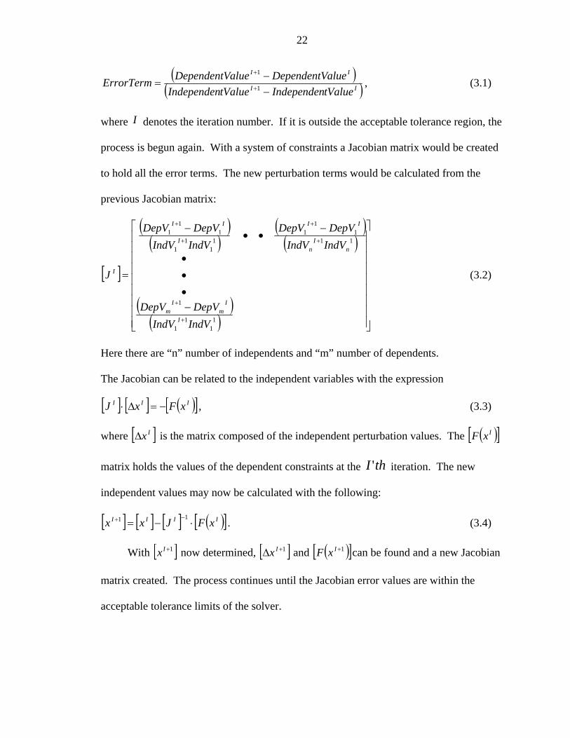
variable to be constrained is a satisfactory one. A partial derivative error term is
calculated,
22
( )( )II
II
tValueIndependentValueIndependenalueDependentValueDependentVErrorTerm
−−
= +
+
1
1
, (3.1)
where I denotes the iteration number. If it is outside the acceptable tolerance region, the
process is begun again. With a system of constraints a Jacobian matrix would be created
to hold all the error terms. The new perturbation terms would be calculated from the
previous Jacobian matrix:
[ ]
( )( )
( )( )
( )( ) ⎥
⎥⎥⎥⎥⎥⎥⎥⎥
⎦
⎤
⎢⎢⎢⎢⎢⎢⎢⎢⎢
⎣
⎡
−•••
−••
−
=
+
+
+
+
+
+
11
11
1
111
11
11
11
11
1
IndVIndVDepVDepV
IndVIndVDepVDepV
IndVIndVDepVDepV
J
I
Im
Im
nI
n
II
I
II
I (3.2)
Here there are “n” number of independents and “m” number of dependents.
The Jacobian can be related to the independent variables with the expression
[ ] [ ] ( )[ ]III xFxJ −=Δ⋅ , (3.3)
where [ ]IxΔ is the matrix composed of the independent perturbation values. The ( )[ ]IxF
matrix holds the values of the dependent constraints at the thI ' iteration. The new
independent values may now be calculated with the following:
[ ] [ ] [ ] ( )[ ]IIII xFJxx ⋅−=−+ 11 . (3.4)
With [ ]1+Ix now determined, [ ]1+Δ Ix and ( )[ ]1+IxF can be found and a new Jacobian
matrix created. The process continues until the Jacobian error values are within the
acceptable tolerance limits of the solver.

23
Figure 3-1 Example NPSS engine model [19]

24
HPT Recuperator
NPSS Code/Element Representation of Above Engine State
HPT FlowStart
Recuperator
RecuperatorFlowEnd
HPT FlowStartEn
Simplified Code Representation
7a 7b
7a 7b
7temp
Figure 3-2 State 7 of HPRTE engine cycle

25
CHAPTER 4 CYCLE CONFIGURATIONS AND BASE POINT ASSUMPTIONS
Before discussing the thermodynamics relationships used in the analysis, it is
necessary to give an overview of the cycles from a systems standpoint. This analysis
compares the design point performance of three engine configurations. The first engine
is a simple cycle gas turbine engine (SCGT). It has been modeled to predict the
performance of the production engine, ETF-40B, which powers the military LCAC for
the United States Navy. The SCGT will be compared to two variations of the HPRTE
engine, the base HPRTE and a variant that uses refrigeration capacity to cool the high
pressure compressor inlet stream.
Major Model Features
When comparing engine systems, it is convenient to understand the major features
of each model. Listed in Table 4.1 is a breakdown of the features that distinguish the
engine configurations from one another. The HPRTE cycles are two spool engines with
exhaust gas product heat recuperation. Both are semi-closed and have compressor inter-
cooling. The H-V Efficiency has additional cooling capacity provided by a vapor
absorption refrigeration system (VARS). The additional cooling enables exhausted water
vapor to be condensed and collected for use elsewhere or for injection after the high
pressure compressor.

26
Flow Path Descriptions & Schematics
Simple Cycle Gas Turbine Engine Model
As mentioned earlier, the SCGT is a simple, open cycle gas turbine engine. For
this analysis the model with have a total of five flow stations (Figure 4-1). State 1 is the
inlet stream. From State 1 to 2 the flow undergoes an adiabatic compression process in
compressor, C1. From State 2 to 3 there is a constant area, premixed burner, B. The
process from State 3 to 4 is an adiabatic expansion process through the turbine, T1.
Mechanical work generated by the turbine drives the compressor and supplies power for
the ship propellers or lift fans. State 5 is the fuel flow station. JP-4 was the fuel of
choice for this analysis because it is widely used in industry and has a high availability.
High Pressure Regenerative Turbine Engine Efficiency Model
Figure 4-2 is a schematic representation for the Efficiency and Power modes of the
HPRTE cycle. The Power mode concept incorporates a flow splitter to bypass some
exhaust from the high pressure turbine and send it directly to the low pressure turbine.
Initially, the Power mode had been considered for this project to give additional boost
capabilities to the low pressure spool. However, while completing the analysis it was
determined that the Efficiency mode predicts sufficient boost for the system and any
additional boost pressure would result in a turbocharger design outside of modern
technology limits.
There are 14 states for the basic HPRTE (the Power mode has 16). Air enters at
State 1 and undergoes an adiabatic compression process in the low pressure compressor,
LPC, before reaching State 2. Next, the fresh air from State 2 is combined with the
recirculated exhaust gas products from State 10 in an isobaric, adiabatic mixing process.
The resultant State is 2.9. Now the combined flow passes through a sea water cooled
27
heat exchanger called the main gas cooler (MGC). The effectiveness, pressure drop, and
process fluid temperature are all given. The resulting State is 3.0. After the gas has been
cooled it goes through another adiabatic compression process in the high pressure
compressor, HPC. The resultant State 4 has the maximum system pressure. Following
the HPC there is a heat recuperation process (RHX) in which high-temperature exhaust
gas product stream preheats the State 4 flow resulting is State 5. From state 5 to 6 the gas
is mixed with fuel and ignited in the combustion chamber, B. A small pressure drop is
applied before State 6 to simulate friction losses in the combustor. The high pressure
turbine inlet temperature, or TIT, was chosen to be 2500°R—an acceptable value for a
medium size engine.
The expansion across the high pressure turbine, HPT, produces the power to drive
the HPC and the net BHP is available power for the vessel. State 7 is State 7.11 in the
Efficiency mode, and that flow passes through the RHX, rejecting heat to State 4. The
only flow splitter for the Efficiency cycle comes at State 9. Here, a user defined
recirculation ratio determines the mass flow rates at State 7.15 and 10. State 10
recombines with fresh air flow from the LPC exit. State 7.2 is also State 7.3 in Efficiency
mode. The final expansion process across the low pressure turbine, or LPT, exhausts to
the environment at State 8.
High Pressure Regenerative Turbine Engine with Vapor Absorption Refrigeration System Efficiency Model
Figure 4-3 is a schematic representation of the H-V Efficiency. The HPRTE-
VARS modes differs from the HPRTE modes only by the addition of two heat
exchangers in the flow path after the recirculated gas products combine with the fresh
inlet air at State 2.9. The generator (GEN) and the evaporator (EVP) are two of the heat

28
exchangers that make up part of the VARS. A schematic of the VARS is also included as
Figure 4-4 for clarification. It was not modeled since the scope of this analysis only
included modeling the gas path side of the combined cycle system. The point of water
collection is shown on the figure, as well. The computational model of this cycle
required the addition of a separator element to perform the water extraction. The
separator is discussed in Chapter 5, Thermodynamic Modeling and Analysis.
Notice that the HPRTE cycles require an iterative solution method to obtain model
convergence because of the semi-closed operation. For the first iteration of the engine
cycle an initial guess for the temperature at State10 is given.
Simple Cycle Gas Turbine Engine Design Assumptions and HPRTE Cycles Base Point Assumptions
The SCGT is a medium size, open-cycle gas turbine engine modeled after the ETF-
40B. The ETF-40B has a seven stage axial compressor followed by a single stage
centrifugal compressor yielding an overall pressure ratio of 10.4 [Robert Cole]. The
nominal output shaft horsepower is 4000 SHP. Turbine inlet temperature was assumed to
be 2500°R. Turbomachinery efficiency information was provided by Dan Brown of
Brown Turbine Technologies. All other engine design parameters were chosen based on
conservative current technology limits. See Table 4-2 for complete details.
The base point HPRTE component parameters are listed in Table 4-3. The same
methodology used to determine the design parameters for SCGT was considered when
deciding base-line design values for the HPRTE engine cycle configurations—size and
technology limitations were applied.
There were material and computational limitations that existed and needed to be
accounted for to preserve the fidelity of the engine model. They are as follows: TIT

29
maximum was 2500°R, hot side recuperator inlet temperature maximum was 2059°R,
turbocharger pressure ratio maximum was 7.5, and HPC inlet temperature minimum was
491°R (NPSS limitations).
Table 4-1 Comparison of major configuration features
SCGTHPRTE Efficiency * * * *H-V Efficiency * * * * * *
Model FeaturesIntercooled
CompressorsVARS cooling
Water ExtractionModel Semi-Closd Turbocharger
Pressurized Recuperatored
1 2 3 4B
C1 T1
5Fuel
Air
Figure 4-1 Simple Cycle Gas Turbine (SCGT) engine model configuration
30
Figure 4-2 High Pressure Regenerative Turbine Engine model, both efficiency and power configurations represented
77.
12
7.2
7.3
86
54
32.
92
1
109
7.11
LPC
RH
X
HPC
MG
CH
PTB
LPT
Fuel
Air
Sea
Wat
er

31
Figure 4-3 High Pressure Regenerative Turbine Engine-Vapor Absorption Refrigeration System, both efficiency and power model configurations represented
77.
12
7.2
7.3
86
54
32
1
109
7.11
2.91
2.92
2.9
LPC
MG
CH
PC
RH
X
BH
PTLP
TG
ENEV
P
Fuel
Air
Wat
e
Sea
Wat
erH
P R
efrig
eran
tLP
Ref
riger
ant
32
GEN
EVP
CND
CND
2.9 2.91
2.923
PumpExpander
Figure 4-4 Vapor Absorption Refrigeration Cycle with HPRTE flow connections
Table 4-2 Simple Cycle Gas Turbine engine design point parameters Parameter ValueC1 Adiabatic Efficiency 0.858Burner Efficiency 0.99Burner Pressure Drop 0.03Turbine Inlet Temperature 2500°RT1 Adiabatic Efficiency 0.873
Table 4-3 Base case model assumptions for HPRTE cycles [3], [26], [27] Parameter Value
Ambient Temperature 544.67°RSea Water Temperature 544.67°R
Ambient Pressure 14.7 PSILPC Adiabatic Efficiency 0.83
GEN Effectiveness 0.85GEN Pressure Drop 0.03MGC Effectiveness 0.85MGC Pressure Drop 0.03EVP Effectiveness 0.85EVP Pressure Drop 0.03
HPC Adiabatic Efficiency 0.858RHXEffectiveness 0.85
RHX Pressure Drop State 4-5 0.04RHX Pressure Drop State 7.11-9 0.04
B Efficiency 0.99B Pressure Drop 0.03
HPT Inlet Temperature 2500°RHPT Adiabatic Efficiency 0.873
Recirculation Ratio 3LPT Adiabatic Efficiency 0.87
Fuel Hydrogen to Carbon Ratio 1.93:1

33
CHAPTER 5 THERMODYNAMIC MODELING AND ANALYSIS
Chapters 3 and 4 addressed the computational structure of NPSS and the cycle
configurations of the models including the design point assumptions. While top level
NPSS calculations are performed by the solution solver, the intermediate operations
performed during every iterative pass to calculate the thermodynamic states are discussed
next. Chapter 5 develops the theory for these auxiliary thermodynamic relations that
drive the model elements (subroutines). These relations are developed using fundamental
thermodynamic concepts.
Thermodynamic Elements
Heat Exchangers
Heat exchangers are an important component in HPRTE cycles. The base HPRTE
Efficiency model mode has two heat exchangers, MGC and RHX; and the combined
cycle, H-V Efficiency, has four heat exchanger elements including three for compressor
inter-cooling. Those for the inter-cooling have defined process inlet flow states. Mass is
conserved by setting the exit mass flow rate equal to the entrance mass flow rate.
User defined inputs include effectiveness, ε , and 1_0 inPPΔ . Let effectiveness be
defined as
( ) ( )( ) ( )
( ) ( )( ) ( )2_01_011
1_01_011
__0__0min_min
__0__0_
max ininpin
outinpin
incoldinhotp
outhotinhothotphot
TTCmTTCm
TTCmTTCm
−⋅
−⋅=
−⋅
−⋅==
&
&
&
&
&
&ε (5.1)
hotpC _ is the hot side specific heat at constant pressure, and min_pC is the specific heat of
the minimum capacity flow stream.

34
Therefore, ( )( )2_01_0
1_01_0
inin
outin
TTTT
−
−=ε . (5.2)
The only unknown in Equation 5.2 is 1_0 outT .
The capacity of the process fluid is set such that it is always the maximum capacity
stream. This ensures that it is not used in the calculation above.
The exit pressure is determined using the following equation:
( )1_01_01_0 1 ininout PPPP Δ−⋅= . (5.3)
Know known are the parameters 1_0 outT , 1_0 outP , and 1outm& . The exit state is set.
Mixers
The mixer is modeled as an adiabatic, constant static pressure process. Because
there is no consideration given for Mach number effects, the stagnation pressures of the
two flows entering the mixer must be identical. This requires a model constraint be set
up by the user for each HPRTE model and satisfied by the solution solver. All HPRTE
models have recirculation mixers which are tasked with combing the recirculated exhaust
gas products with fresh air discharged from the low pressure compressor.
A mass balance requires:
21 ininout mmm &&& += (5.4)
Assuming adiabatic mixing, the energy balance is as follows:
out
ininininout m
hmhmh
&
&& 2_021_01_0
+= . (5.5)
Constant pressure mixing implies:
outinin PPP _02_01_0 == . (5.6)

35
Other parameters such as the outFAR and the mass fractions are mass averaged. For
example:
out
ininininout m
FARmFARmFAR
&
&& 2211 += . (5.7)
With outh _0 , outP _0 , outm& , and the exit state mass fractions all known, all other
thermodynamic properties can be found.
Splitter
In Chapter 4 the cycle schematics for the HPRTE cycle models showed flow
splitting occurring at State 9. To accomplish this feature with a computer model a splitter
component must be defined to separates flow into two streams before exhausting to the
environment. The recirculation splitter is tasked with the job of splitting the flow stream
on a mass basis after the high temperature recuperation process (State 9). A portion of
the flow is reconstituted with fresh air before heading back through the core engine
components while the rest is directed to the low pressure turbine (LPT) to power the
turbocharger. A bypass ratio, BPR, is user defined to represent the mass basis split of the
flow streams. The recirculation splitter inlet state is defined by the following know
parameters: inT _0 , inP _0 , intotm _& , inFAR , inh _0 , and mass fractions for all species.
In general BPR is defined as
1_
2_
outtot
outtot
mm
BPR&
&= . (5.8)
For this application the bypass ratio is defined as
exhaustedtot
recirctotcirc m
mBPR
_
_Re &
&= . (5.9)

36
recirctotm _& is the mass flow rate recirculated and mixed with fresh air. exhaustedtotm _& is
the mass flow rate that passes directly to the low pressure turbine and be exhausted from
the system at State 8.
The user also reserves the option of applying flow pressure drops to either or both
of the split streams, but for this analysis the splitter is modeled as an isobaric process.
Similarly, the process is adiabatic, as there is no heat transfer. The mass fractions are
unchanged; therefore, the exit state of each flow is defined.
inoutout PPP _02_01_0 == (5.10)
inoutout TTT _02_01_0 == (5.11)
Water Extractor
The water extraction component is only present in the H-V Efficiency
configuration. Because water vapor is present in the recirculated mixed gases and the
cooling capacity of the three heat exchangers is significant to cause condensation to occur
in the flow stream, it is desirable to separate the liquid water from the gas flow before the
inlet to the high pressure compressor. The separation of liquid water from the flow
stream is modeled as an isentropic process. The inlet state is completely defined;
therefore, liquidOHm _2& and liquidOHh _2 are readily available from CEA. The exit state is
defined by first setting the inlet and exit temperatures and pressures equal.
inout PP _0_0 = (5.12)
inout TT _0_0 = (5.13)
Then the exit mass flow rate and enthalpy are set.
liquidOHintotouttot mmm _2__ &&& −= (5.14)

37
liquidOHinout hhh _2_0_0 −= (5.15)
The exit state of the water extractor is now defined.
Compressors
Compressors inlet states are defined with the following parameters passed to the
element: inT _0 , inP _0 , intotm _& , inFAR , inh _0 , and mass fractions for all species. The
performance of the compressor is determined by the following parameters: pressure ratio
( CompPR ) and adiabatic efficiency ( adComp _η ).
Exit pressure is determined first with the equation
inCompout PPRP _0_0 ⋅= . (5.16)
The other thermodynamic parameter, the adiabatic efficiency, is used to calculate
the exit state point parameters in the NPSS Compressor module. Define the adiabatic
compressor efficiency as
inout
inidealoutadComp hh
hhworkcompressoradiabatic
workcompressorideal
_0_0
_0__0_ __
__−
−==η . (5.17)
Determining the ideal exit state enthalpy is straight forward knowing outP _0 and
idealouts __0 if idealoutin ss __0_0 = . Since entropy and enthalpy are only functions of
temperature; the exit state ideal temperature is quickly found along with enthalpy. Now,
rearrange and directly solve Equation 5.17 for outh _0 . With the exit pressure and
enthalpy know known, all exit state thermodynamic parameters are readily calculated by
CEA.
The power required by the compressor is also calculated.
outoutininComp hmhmW _0_0_0_0 ⋅−⋅= &&& (5.18)

38
The power is converted from Btu/sec to HP:
HP
lbfftBTU
lbfftWComp
1sec
5501
778
⋅
⋅⋅& . (5.19)
Polytropic efficiency, polyComp _η , is an output parameter calculated from the
entrance and exit entropies and pressures. The derivation is as follows:
The definition of the polytropic efficiency is
dhdhi
polyComp =_η . (5.20)
To arrive at this equation, first consider a reversible form of the energy equation.
Since PdvvdPdudh ++= , (5.21)
vdPdhPdvvdPPdvdhPdvduTds −=+−−=+= )( (5.22)
Therefore, P
dPRTdhdP
Tv
Tdhds −=−= . (5.23)
Solving Equation 5.23 for Tdh yields
PdPRds
Tdh
+= . (5.24)
For an isentropic process 0=ds . Therefore,
PdPR
Tdhi = . (5.25)
Combining Equations 5.24 and 5.25 results in the following:
PdPRds
PdPR
Tdh
Tdh
dhdh i
ipolyComp
+===_η . (5.26)
Integrating Equation 5.26 from the inlet state to the exit state yields:

39
( )( )CompinCompinout
CompinComppolyComp PRRss
PRRlog
log
__0_0
__ ⋅+−
⋅=η . (5.27)
Turbines
Turbines provide the power to drive the compressors as well as the net power for
the ship propellers and lift fans (if LCAC is the mission). The NPSS model Turbine
element requires a defined entrance state to include such parameters as inT _0 , inP _0 ,
intotm _& , inFAR , inh _0 , and mass fractions for all species present. As was the case with the
compressors, the performance of the turbine components is determined by the defined
parameters: pressure ratio ( TurbPR ) and adiabatic efficiency ( adTurb _η ). NPSS defines
TurbPR differently than most turbomachinery reference texts. Here it is defined as:
out
inTurb P
PPR
_0
_0= . (5.28)
The exit state can be determined by first applying the turbine pressure ratio.
Turb
inout PR
PP _0
_0 = . Turbinout PRPP _0_0 = (5.29)
As was the case for the compressor, outh _0 is the other thermodynamic parameter
necessary to in order to define the exit state. The turbine adiabatic efficiency is defined
as:
idealoutin
outinadTurb hh
hhworkturbineideal
workturbineadiabatic
__0_0
_0_0_ __
__−
−==η . (5.30)
The power generated by the turbine is also calculated.
outoutininTurb hmhmW _0_0_0_0 ⋅−⋅= &&& (5.31)
40
This power is converted to horsepower as it is in the compressor. The polytropic
efficiency is an output parameter calculated using the same approach described in the
compressor section. The final equation is given below.
( )( )TurbinTurb
TurbinTurbinoutpolyTurb PRR
PRRss/1log
/1log
_
__0_0_ ⋅
⋅+−=η (5.32)
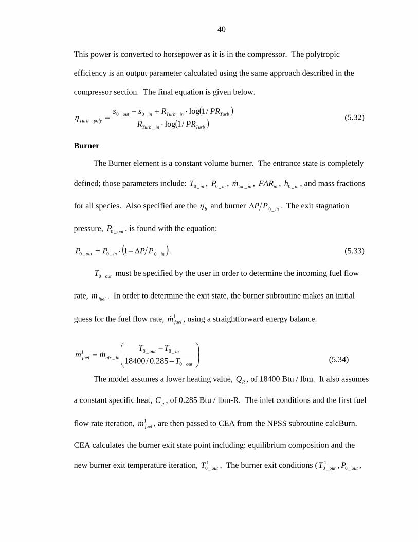
Burner
The Burner element is a constant volume burner. The entrance state is completely
defined; those parameters include: inT _0 , inP _0 , intotm _& , inFAR , inh _0 , and mass fractions
for all species. Also specified are the bη and burner inPP _0Δ . The exit stagnation
pressure, outP _0 , is found with the equation:
( )ininout PPPP _0_0_0 1 Δ−⋅= . (5.33)
outT _0 must be specified by the user in order to determine the incoming fuel flow
rate, fuelm& . In order to determine the exit state, the burner subroutine makes an initial
guess for the fuel flow rate, 1fuelm& , using a straightforward energy balance.
(5.34)
The model assumes a lower heating value, RQ , of 18400 Btu / lbm. It also assumes
a constant specific heat, pC , of 0.285 Btu / lbm-R. The inlet conditions and the first fuel
flow rate iteration, 1fuelm& , are then passed to CEA from the NPSS subroutine calcBurn.
CEA calculates the burner exit state point including: equilibrium composition and the
new burner exit temperature iteration, 1_0 outT . The burner exit conditions ( 1
_0 outT , outP _0 ,
⎟⎟⎠
⎞⎜⎜⎝
⎛
−
−=
out
inoutinairfuel T
TTmm
_0
_0_0_
1
285.0/18400&

41
outFAR , outWAR , outh _0 , and mass fractions for all species) are then passed back to
calcBurn where the burner efficiency is applied to determine the actual burner exit
temperature, actoutT _1
_0 .
( ) ininoutbactout TTTT _0_0
1_0
_1_0 +−=η (5.35)
Then, actoutT _1
_0 is used to determine the next fuel flow rate iteration, 2fuelm& , with the
energy balance described above (Equation 5.34). An error check is performed on the fuel
flow rate values every iteration to determine when the loop can be exited.
ToleranceErrormmm fuelfuelerrorfuel _12_ ≤−= &&& (5.36)
Once fuelm& is determined, the exit state point is completely defined.
Sensitivity Analysis
No formal optimization program was used for this project; instead, each engine
cycle model was roughly optimized manually starting from base case assumptions listed
in Chapter 4. The sensitivity analyses were performed on the SCGT and HPRTE
Efficiency models to determine the influences of particular design parameters. The H-V
Efficiency model was not included in these studies because the results would mirror those
for the HPRTE Efficiency model analysis. Two primary dependent parameters
investigated in the sensitivity analysis include thermal efficiency and specific power.
The thermal efficiency is defined as:
Rfuelth Qm
W⋅
=&
&η , (5.37)
where RQ is the lower heating value of the fuel and W& is the net power.

42
The specific power is defined as: inairm
WSP_&
&= . (5.38)
Influence coefficients are use to quantify the sensitivity of resultant parameters as
they relate to perturbed input parameters. The dimensional influence coefficient is
defined as
( )( )ParameterInput
Resultant∂
∂ . (5.39)
To relate the magnitudes of influence coefficients to one another, they must be non-
dimensionalized is required. This is accomplished by dividing the perturbed value by its
base case quantity:
( )
( )Value BaseParameter Input
ParameterInput Value BaseResultant
Resultant
∂
∂. (5.40)
Such an example of a non-dimensional influence coefficient is given below. Here,
the HPC inlet temperature is perturbed from its base value and the resultant change to thη
is expressed in the following form. A value of 1 suggests that a 1% perturbation in HPC
inlet temperature results in a 1% change in thη . In this way the sensitivity of input
parameters is determined.
( )
base
baseth
th
TinHPCTinHPC
_)_(
_
∂
∂η
η
(5.41)

43
CHAPTER 6 RESULTS AND DISCUSSION
The results and discussion of the analysis performed using the cycle code NPSS are
presented in Chapter 6. The first section in this chapter, Cycle Code Comparison,
compares results from the spreadsheet code (used by Boza [22]) and the NPSS program
for one operating point of the HPRTE Efficiency model. Next, sensitivity studies were
performed on the SCGT and HPRTE Efficiency cycles and influence coefficients were
calculated. Engine model results are given and compared to derived thermodynamic
expressions. Finally, plots and tables are presented that compare the performance
parameters of the three engine configurations.
Cycle Code Comparison
Before initiating the sensitivities studies, it is important to benchmark the NPSS
program and compare results of one model configuration to those results obtained from
running a proven cycle analysis program. One operating point for the HPRTE Efficiency
model was chosen for the comparison, and the results from the two cycle codes are
presented in Table 6-1. The third column in the table lists the absolute differences of the
two data sets parameters in percentages. Agreement of the data between the two codes is
high; values for thη , OPR, HPT exit temperature (TET), inHPCT _ , and exhaustT are all
within acceptable limits. The SpPw calculated by the spreadsheet model was 12.5%
higher than that calculated in NPSS. There are three possible reasons for the disparity in
the output values. First, it is impossible to implicitly balance the low pressure spool

44
specific work; therefore the turbine specific work is never properly matched to the
specific power of the compressor. This could very easily result in a different airm& . Two,
different fuels are used in the codes. The hydrogen-to-carbon ratio is 1.93 in NPSS and
2.03 in the spreadsheet code. Because the fuels are different, the curve-fit coefficients
used to calculate the enthalpies for the spreadsheet code could be different than the ones
used by NPSS.
Sensitivity Analysis
Simple Cycle Gas Turbine Engine Model
Of particular interest for this project is the sensitivity of the open-cycle engine
thermal efficiency and specific power to variations in turbine inlet temperature and
ambient temperature. Figures 6-2 through 6-4 show the results of the analysis. Unless
otherwise specified the following parameters remained constant throughout the analysis:
ambient temperature is 544°R, TIT is 2500°R, and nominal power output is 4000 BHP.
Figure 6-2 displays the thermal efficiency as a function of the overall cycle pressure ratio
(OPR). The TIT variations have a strong influence on the outcome of the thermal
efficiency value. Raising TIT has a positive effect on thη which also implies that the
total heat added to the system has been reduced since the power output remains steady.
Let thη be defined by the following relationship:
Rfuelth Qm
W⋅
=&
&η . (6.1)
Since, RQ , the fuel lower heating value, is constant; fuelm& has to decrease in order
to reduce the total heat added to the system in order to raise the thη . For all run cases in
the SCGT analysis, variations in thη are the direct result of variations in fuelm& .

45
To better understand the relationship between thη and the input parameters in this
sensitivity study, the following derivation has been included. The State numbers in the
equations correspond to those for the SCGT cycle schematic given in the Configurations
chapter (Figure 4-1). Figure 6-1 shows the comparison between the theoretical
expression below, the run data from NPSS, and ideal thermal efficiency expression for an
air standard Brayton cycle available in any thermodynamic text. The derived expression
predicts a curve with higher efficiency than the NPSS output; this is expected because the
pressure losses in the combustor are not accounted for, as it was assumed that the turbine
pressure ratio is equal to the compressor pressure ratio. That and the fact that the specific
heat ratio (γ ) was averaged for the entire cycle may explain the discrepancy between the
results from NPSS and the derived curve-fit expression.
There are several assumptions exercised in this derivation to develop the final
expression in terms of only the following parameters: 01
03
TT
, γ , PR , adTurb _η , and
adComp _η . They are as follows:
fuelm& is much less than airm&
( )Thh =
constant≅pC
ratio of specific heats, constant≅γ
PRPP
PP
=≅04
03
01
02
Beginning with the definition of thermal efficiency:

46
( ) ( )[ ]Rfuel
airp
Rfuelth Qm
TTTTmCQm
W⋅
−−−=
⋅=
&
&
&
& 01020403η . (6.2)
Factoring out 01T gives:
Rfuel
airp
th QmTT
TT
TT
TmC
⋅
⎥⎦
⎤⎢⎣
⎡+−−
=&
& 101
02
01
04
01
0301
η . (6.3)
Now the adiabatic turbomachinery efficiencies derived in the previous chapter may be
rewritten in the form:
⎟⎟⎠
⎞⎜⎜⎝
⎛−
⎟⎠
⎞⎜⎝
⎛ −=
−
1
1
01
02
1
_
TT
PR
adComp
γγ
η . (6.4)
⎟⎠
⎞⎜⎝
⎛ −
⎟⎟⎠
⎞⎜⎜⎝
⎛−
=−
1
1
104
03
_γ
γη
PR
TT
adTurb (6.5)
Solving the compressor Equation 6.4 for 01
02
TT
and Equation 6.5 for 04T yields the
following two expressions.
⎟⎠
⎞⎜⎝
⎛ −+=−
1111
_01
02 γγ
ηPR
TT
adComp
(6.6)
⎟⎟⎟⎟⎟
⎠
⎞
⎜⎜⎜⎜⎜
⎝
⎛
+⎟⎠
⎞⎜⎝
⎛ −=
−
11 _
103
04
adTurbPR
TT
ηγγ
(6.7)
Substituting Equations 6.6 and 6.7 into Equation 6.3 gives the following expression:

47
Rfuel
adCompadTurb
airp
th Qm
PRPRT
TTT
TmC
⋅
⎥⎥⎥⎥
⎦
⎤
⎢⎢⎢⎢
⎣
⎡
⎟⎠
⎞⎜⎝
⎛ −−
⎟⎟⎟⎟⎟
⎠
⎞
⎜⎜⎜⎜⎜
⎝
⎛
+⎟⎠
⎞⎜⎝
⎛ −−
=
−
−
&
& 11
11
1 1
__
101
03
01
0301
γγ
γγ ηη
η (6.8)
The denominator can be rewritten in terms of 01
03
TT
, γ , PR , and adComp _η .
The energy balance of the combustor is as follows:
( ) 030302 TCmTCmmmQTCm pairpfuelairfuelRpair &&&&& ≅+=+ . (6.9)
Now, solving for RfuelQm& gives:
( ) ⎟⎟⎠
⎞⎜⎜⎝
⎛−=−=
01
02
01
03010203 T
TTT
TCmTTCmQm pairpairRfuel &&& . (6.10)
Substituting in the expression for 01
02
TT in Equation 6.6 results in the following:
⎥⎥⎦
⎤
⎢⎢⎣
⎡−⎟
⎠
⎞⎜⎝
⎛ −−=−
111 1
_01
0301
γγ
ηPR
TT
TCmQmadComp
pairRfuel && . (6.11)
The final expression for thη is
⎥⎥⎦
⎤
⎢⎢⎣
⎡−⎟
⎠
⎞⎜⎝
⎛ −−
⎥⎥⎥⎥
⎦
⎤
⎢⎢⎢⎢
⎣
⎡
⎟⎠
⎞⎜⎝
⎛ −−
⎟⎟⎟⎟⎟
⎠
⎞
⎜⎜⎜⎜⎜
⎝
⎛
+⎟⎠
⎞⎜⎝
⎛ −−
=−
−
−
111
11
11
1
1
_01
03
1
__
101
03
01
03
γγ
γγ
γγ
η
ηηη
PRTT
PRPRT
TTT
adComp
adCompadTurb
th . (6.12)
As mentioned above, the ideal thermal efficiency for an air standard Brayton is also
plotted on Figure 6.1.

48
γγη 1_11 −−=
PRidealth (6.13)
Simple Cycle Gas Turbine Engine Model Sensitivity Analysis
Figure 6.2 is a plot of the thermal efficiency as a function of OPR with separate
curves for TITs. These curves peak at certain OPR values; continuing to increase
pressure ratio will continue to decrease the heat added per unit mass to the cycle,
however, the thermal efficiency will drop because the recuperator capacity to exchange
heat is being neutralized. When this happens the thermal efficiency begins to drop again.
The influence coefficients were determined for Figure 6.2. The base case engine
chosen had a TIT of 2500°R with an OPR of 24. These numbers imply that changes in
TIT effect greater change in thη than changes in OPR. One other point to note is the fact
that no matter what the TIT is for the engine model, the maximum thermal efficiency
always occurs when the compressor power is about twice as large as the net BHP.
( )898.0
)(_ =
∂
∂
base
baseth
th
TITTIT
ηη
( )0322.0
)(_ =
∂
∂
base
baseth
th
OPROPR
ηη
Figure 6-3 displays specific power sensitivity to changes in TIT over a pressure
range from 8 to 18. The drop in specific power for increasing OPRs can be explained as
follows. Consider the engine as a control volume that produces a constant power output.
Ignoring the small effects to thermal efficiency that increasing OPR produces, the heat
energy added to the engine must be constant. However, as OPR increases the heat rate
per unit mass added in the combustor drops. Therefore, more air must be brought into the
combustor to maintain the total heat energy input required to produce a constant power
engine output. The other trend visible has to do with increasing TIT and its influence on

49
specific power. Drawing two cycles, with different TITs, on the same T-S diagram
clearly demonstrates this phenomenon.
Influence coefficients were calculated using the base case parameters from the last
section. Specific power is more affected by changes in TIT than changes in OPR. In
fact, there is 1 order of magnitude difference between the two parameters. The negative
sign quantifies the drop in specific power with increasing OPR that was discussed earlier.
( )36.3
)(=
∂
∂
base
base
TITTIT
SpPwSpPw
( )339.0
)(−=
∂
∂
base
base
OPROPR
SpPwSpPw
Figure, 6-4 examines operating temperature variation as it influences cycle thermal
efficiency and OPR. The OPR curves are nearly linear and the slopes become more
negative as OPR increases. Notice that the thermal efficiencies approach 40% as ambient
temperature falls to 509°R. Cold day operation translates to good thermal efficiency for
the SCGT. Notice the effect of changing OPR for the case when ambientT is 572°R. The
higher OPR curves collapse on each other implying that thermal efficiency maximums
are at or near their peak values here, and any further boost in OPR drops the thermal
efficiency off the other side of the curve that would appear if this was a three dimensional
figure. For example, at ambientT 554°R, the maximum thermal efficiency corresponds to
an OPR of 24. A further boost to an OPR of 28 results in a reduced thermal efficiency.
The influence coefficients corresponding to Figure 6-4 for thermal efficiency and
specific power are calculated assuming the base case cycle where ambient temperature is
518°R and OPR is 24.

50
( )669.0
)(_ −=
∂
∂
base
baseth
th
TambTamb
ηη
( )0682.0
)(_ =
∂
∂
base
baseth
th
OPROPR
ηη
The thermal efficiency coefficients suggest that drops in ambient operating
temperature impact thermal efficiency more so than variations in pressure ratio. This
implies that OPR is a secondary issue if the engine is being designed with the intent to
optimize thermal efficiency.
( )76.1
)(−=
∂
∂
base
base
TambTamb
SpPwSpPw
( )2676.0
)(−=
∂
∂
base
base
OPROPR
SpPwSpPw
The specific power influence coefficients quantify the negative impact on specific
power when either ambient temperature or OPR is increased. Of course, the effect of
ambient temperature is much more significant—almost an order of magnitude greater.
High Pressure Regenerative Turbine Engine Efficiency Model
Before beginning the sensitivity analysis of the HPRTE Efficiency, it is important
to examine the validity of the data output from NPSS. To accomplish this task an
expression has been derived to test the validity of NPSS output. After the derivation is
complete, the resulting expression is normalized; and it is only a function of the
following parameters: 01
2.07
TT
, LPPR , γ , adLPC _η , and adLPT _η . The plotted NPSS data
should agree with the derived expression. The ten points in Figure 6-5 represent ten
distinct converged operating points from NPSS runs. The standard deviation of the set of
points is 0.00398, signifying close conformity with the derived thermodynamic
expression. The development uses the following assumptions:

51
fuelm& << airm&
( )Thh =
constant≅pC
Ratio of specific heats, constant≅γ
LPPRPP
PP
=≅08
2.07
01
02
The development begins with the adiabatic efficiency expressions for the low pressure
compressor and turbine:
⎟⎟⎠
⎞⎜⎜⎝
⎛−
⎟⎠
⎞⎜⎝
⎛ −=
−
1
1
01
02
1
_
TT
LPPR
adLPC
γγ
η (6.14)
⎟⎠
⎞⎜⎝
⎛ −
⎟⎟⎠
⎞⎜⎜⎝
⎛−
=−
1
1
108
2.07
_γ
γη
LPPR
TT
adLPT . (6.15)
Solving Equation 6.14 for 01
02T
T yields
⎟⎠
⎞⎜⎝
⎛ −⎟⎟⎠
⎞⎜⎜⎝
⎛=−
−
1111
_01
02 γγ
ηLPPR
TT
adLPC
. (6.16)
Now, introducing the power balance for the turbocharger gives
( ) ( )082.070102 )( TTCmmTTCm pfuelinpin −+=− &&& . (6.17)
And simplifying Equation 6.17 using the assumptions provided above results in
( ) ( )082.070102 TTTT −=− . (6.18)

52
Rearranging Equation 6.18 and solving for 101
02 −TT produces
⎟⎟⎠
⎞⎜⎜⎝
⎛−=−
01
08
01
2.07
01
02 1TT
TT
TT
. (6.19)
Setting Equation 6.16 equal to Equation 6.19 gives
⎟⎟⎠
⎞⎜⎜⎝
⎛−=⎟
⎠
⎞⎜⎝
⎛ −⎟⎟⎠
⎞⎜⎜⎝
⎛ −
01
08
01
2.071
_
11TT
TT
LPPRadLPC
γγ
η. (6.20)
Solving Equation 6.20 for 08T produces
⎥⎥⎦
⎤
⎢⎢⎣
⎡⎟⎠
⎞⎜⎝
⎛ −⎟⎟⎠
⎞⎜⎜⎝
⎛−⎟⎟
⎠
⎞⎜⎜⎝
⎛=
−
11 1
_01
2.070108
γγ
ηLPPR
TT
TTadLPC
. (6.21)
Next, rearranging Equation 6.15 and solving for 08T yields
111
_
2.0708
+⎟⎠
⎞⎜⎝
⎛ −=
−γ
γ
η LPPR
TT
adLPT
. (6.22)
Setting Equation 6.21 equal to Equation 6.22 results in the following expression:
⎥⎥⎦
⎤
⎢⎢⎣
⎡⎟⎠
⎞⎜⎝
⎛ −⎟⎟⎠
⎞⎜⎜⎝
⎛−⎟⎟
⎠
⎞⎜⎜⎝
⎛=
+⎟⎠
⎞⎜⎝
⎛ −
−
−11
11
1
_01
2.07011
_
2.07 γγ
γγ ηη
LPPRTT
TLPPR
T
adLPCadLPT
. (6.23)
Rearranging,
⎥⎦
⎤⎢⎣
⎡+⎟
⎠
⎞⎜⎝
⎛ −⋅⎥⎥⎦
⎤
⎢⎢⎣
⎡⎟⎠
⎞⎜⎝
⎛ −⎟⎟⎠
⎞⎜⎜⎝
⎛−⎟⎟
⎠
⎞⎜⎜⎝
⎛=
−−
1111 1
_
1
_01
2.07
01
2.07 γγ
γγ
ηη
LPPRLPPRTT
TT
adLPTadLPC
. (6.24)
Then dividing both sides by 01
2.07
TT
yields the final expression plotted in Figure 6-5.
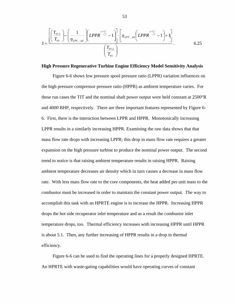
53
⎟⎟⎠
⎞⎜⎜⎝
⎛
⎥⎦
⎤⎢⎣
⎡+⎟
⎠
⎞⎜⎝
⎛ −⋅⎥⎥⎦
⎤
⎢⎢⎣
⎡⎟⎠
⎞⎜⎝
⎛ −⎟⎟⎠
⎞⎜⎜⎝
⎛−⎟⎟
⎠
⎞⎜⎜⎝
⎛
=
−−
01
2.07
1
_
1
_01
2.07 1111
1
TT
LPPRLPPRTT
adLPTadLPC
γγ
γγ
ηη
. 6.25
High Pressure Regenerative Turbine Engine Efficiency Model Sensitivity Analysis
Figure 6-6 shows low pressure spool pressure ratio (LPPR) variation influences on
the high pressure compressor pressure ratio (HPPR) as ambient temperature varies. For
these run cases the TIT and the nominal shaft power output were held constant at 2500°R
and 4000 BHP, respectively. There are three important features represented by Figure 6-
6. First, there is the interaction between LPPR and HPPR. Monotonically increasing
LPPR results in a similarly increasing HPPR. Examining the raw data shows that that
mass flow rate drops with increasing LPPR; this drop in mass flow rate requires a greater
expansion on the high pressure turbine to produce the nominal power output. The second
trend to notice is that raising ambient temperature results in raising HPPR. Raising
ambient temperature decreases air density which in turn causes a decrease in mass flow
rate. With less mass flow rate to the core components, the heat added per unit mass to the
combustor must be increased in order to maintain the constant power output. The way to
accomplish this task with an HPRTE engine is to increase the HPPR. Increasing HPPR
drops the hot side recuperator inlet temperature and as a result the combustor inlet
temperature drops, too. Thermal efficiency increases with increasing HPPR until HPPR
is about 5.1. Then, any further increasing of HPPR results in a drop in thermal
efficiency.
Figure 6-6 can be used to find the operating lines for a properly designed HPRTE.
An HPRTE with waste-gating capabilities would have operating curves of constant

54
HPPR; therefore, the horizontal grid lines on the Figure 6-6 could be called operating
curves as well. Moreover, the line corresponding to a HPPR of 5.1 would represent the
highest thermal efficiency operating curve.
The influence coefficients for Figure 6-6 are listed below. The base case has an ambient
temperature of 528°R and a LPPR of 6.0. ambientT and LPPR variations both have
significant resultant effects on HPPR. Operationally speaking, ambientT is related to airm&
which can cause large changes to the specific power of the system.
( )63.1
)(=
∂
∂
base
base
LPPRLPPR
HPPRHPPR
( )
15.6)(
=∂
∂
base
base
TambTamb
HPPRHPPR
Figure 6-7 shows cycle thermal efficiency sensitivity to TIT variation for a range of
HPPRs. The analysis holds R, ambient temperature, output shaft horse power, and all
component efficiencies constant. NPSS convergence is difficult to achieve if HPPR is
changed manually by the user; instead, to effect change in HPPR, the LPPR is controlled
by the modeler. As LPPR was increased, the model solver reduced fresh air flow rate to
the engine. The mass flow rate reduction caused the HPPR to rise for the same reason
discussed in the previous section. Figure 6-6 shows that the thermal efficiency peaks
very close to an HPPR of 5.1. Along a curve, TET and the stoichiometry change because
R is held constant.
The influence coefficients for thη and SpPw were produced by making
perturbations around the base run case where TIT was 2500°R and HPPR was 5.12.
( )847.0
)(_ =
∂
∂
base
baseth
th
TITTIT
ηη
( )0106.0
)(_ −=
∂
∂
base
baseth
th
HPPRHPPR
ηη

55
The interpretation of these influence coefficients suggests that changing TIT by 1%
causes a 0.847% change in thη . The second coefficient was calculated with data taken
from the right side of the plot where HPPR is monotonically increasing and thη continues
to decrease. The small coefficient value suggests that a large change in HPPR has only
limited effect on thη . This is expected when the influence coefficient is calculated near
an optimum thη point on the curve. Below, notice that TIT perturbations cause
significant resultant changes to the value of specific power.
( )59.2
)(=
∂
∂
base
base
TITTIT
SpPwSpPw
( )
318.0)( =∂
∂
base
base
HPPRHPPR
SpPwSpPw
Figure, 6-8 shows the importance with respect to thermal efficiency of reducing the
HPC inlet temperature for HPRTE engine cycles. Sensitivity to circBPRRe is shown and
its value is varied from 2.0 to 3.5. Those parameters held constant for the analysis are as
follows: output BHP, ambientT , TIT, LPPR, all turbomachinery efficiencies, and the sea
water temperature. The HPC inlet temperature was varied by changing the effectiveness
of the main cooler. The trend toward higher thermal efficiencies for lower HPC inlet
temperatures is the same phenomenon seen in Figure 6-4. A lower inlet temperature to
the high pressure core results in an increase in predicted thermal efficiency. Examination
of the model data used to produce Figure 6-8 shows that as HPC inlet temperature drops,
HPPR increases. As a result the temperature change across the HPT increases and the
mass flow requirements drop. This in turn means that the fuel flow requirement is less.
As shown by Equation 6.1, the drop in fuel flow directly affects thermal efficiency since

56
power output is constant. Lower circBPRRe helps thermal efficiency because TIT must be
maintained at 2500°R. The more inert combustion products that are mixed with fresh air
act to drive down TIT making it necessary to burn more fuel to keep TIT constant.
However, higher recirculation boosts specific power as less fresh air is required to
produce the desired power output. The ultimate choice is the designer’s—if weight and
compactness are important, circBPRRe would be maximized. However, on a naval vessel,
weight might not be the paramount consideration.
The influence coefficients for thη and SpPw are calculated using the base case
circBPRRe of 3 and a HPC inlet temperature of 622°R.
( )58.1
_)_(
_ −=∂
∂
base
baseth
th
TinHPCTinHPC
ηη
( )0610.0
)(_ −=
∂
∂
base
baseth
th
RRη
η
( )66.3
_)_(
−=∂
∂
base
base
TinHPCTinHPC
SpPwSpPw
( )624.0
)(=
∂
∂
base
base
RR
SpPwSpPw
The influence coefficients based on variations to circBPRRe help to quantify the
effects on thermal efficiency and specific power that were discussed above. Moreover,
reducing the HPC inlet temperature boosts both thermal efficiency and specific power.
This is an observed behavior in recuperated gas turbine engines.
Figure 6-9 displays the thermal efficiency sensitivity to pressure drops in the
coolers. To obtain the curves below, HPT exit temperature variations were created by the
modeler. This was done in the same manner as it was for the Figure 6-7. LPPR was
manually controlled to effect change in HPC pressure ratio which caused the HPT exit
temperature to change.

57
The general trends are consistent with the results of Figure 6-7. The curve of
Figure 6-7 corresponding to that of a TIT of 2500°R is the same as the curve in Figure 6-
9 for a cooler PPΔ of 3%. There the HPT exit temperature is 1884°R. The propensity
to see a lowered thermal efficiency when the cooler PPΔ is raised has a straightforward
explanation. Increasing cooler PPΔ results in a drop in the OPR of the cycle. Since the
net output power remains constant, mass flow must be increased. This in turn causes a
rise in fuel flow rate and a drop in thermal efficiency.
Influence coefficients for cooler PPΔ and HPT exit temperature are listed below
for the base cycle case where cooler PPΔ is 3% and HPT exit temperature is 1884°R.
Specific power influence coefficients are included. The results show that neither cooler
PPΔ nor HPT exit temperature affect significant change in thermal efficiency.
However, the specific power is positively influenced by decreasing HPT exit
temperature.
( )0258.0
/)/(
_ −=
ΔΔ∂
∂
base
baseth
th
PPPPη
η
( )0617.0
_)_(
_ =∂
∂
base
baseth
th
TexitHPTTexitHPT
ηη
( )0407.0
/)/(
−=
ΔΔ∂
∂
base
base
PPPP
SpPwSpPw
( )86.1
_)_(
−=∂
∂
base
base
TexitHPTTexitHPT
SpPwSpPw
Figure 6-10 considers specific power sensitivity to HPC adiabatic efficiency. For
an engine with constant power output and TIT, raising TET also results in core mass flow
increasing. That is because a higher low pressure recuperator inlet temperature drives the
combustor inlet temperature up. The effect of driving that temperature up is similar to
what happens for SCGT when OPR is increased. While the total heat added to the engine

58
may be remain almost constant, the heat added per unit mass drops off as combustor inlet
temperature rises. Consequently, the mass flow coming into the combustor must go up.
The result is a drop in specific power. The other noteworthy trend here is the positive
effect on specific power that comes from raising HPC adiabatic efficiency. Raising HPC
adiabatic efficiency decreases the power requirement of the HPC thereby increasing the
specific power of the cycle.
Influence coefficients are considered for a base engine with HPC adiabatic
efficiency of 86 % and HPT exit temperature of 1883°R. Both thermal efficiency and
SpPw influence coefficient are given. Compare these results with the influence
coefficients for the cooler PPΔ discussed above. The adComp _η has a stronger effect on
the performance of the cycle than does PPΔ .
( )06.1
)(_
_
_ =∂
∂
baseadComp
adComp
baseth
th
ηη
ηη
( )74.1
)(_
_=
∂
∂
baseadComp
adComp
baseSpPwSpPw
ηη
Figure 6-11 is a sister plot to Figure 6-10. It describes the same specific power
trends, however, now they are in terms of HPC pressure ratio (HPPR). HPT adiabatic
efficiency ( adTurb _η ) is varied to show specific power sensitivity to this parameter. The
expectation for high adTurb _η to result in an improved specific power is met. From a
thermodynamic standpoint, higher adTurb _η means a greater temperature drop across the
turbine for the same HPPR. Therefore, less mass flow is required to produce the same
power—resulting in a boosted specific power.

59
Influence coefficients for SpPw and thη were calculated from the base cycle case
where adTurb _η was 87% and HPPR was roughly 5.1. Note: since HPPR is an output, it
can not be explicitly set. The coefficient values imply significant influence of adTurb _η on
thη and SpPw . Similarly, notice that the coefficients calculated based on HPPR
variation are very close to those same coefficients calculated for Figure 6-7 when TIT
was the sensitivity parameter. In fact, there is less than a 1% difference between the
values.
( )0105.0
)(_ −=
∂
∂
base
baseth
th
HPPRHPPR
ηη
( )46.1
)(_
_
_ =∂
∂
baseadTurb
adTurb
baseth
th
ηη
ηη
( )316.0
)(=
∂
∂
base
base
HPPRHPPR
SpPwSpPw
( )36.2
)(_
_=
∂
∂
baseadTurb
adTurb
baseSpPwSpPw
ηη
Figure 6-12 displays exhaust gas temperature sensitivity to OPR with TIT
variations included. Cycle constants included: output BHP, LPPR, ambient temperature,
R, and all component efficiencies except for MCG effectiveness. Since LPPR was held
constant, MCG effectiveness was varied to effect HPPR change. The results indicate that
exhaust gas temperature is not sensitive to either OPR or TIT variation. This should be
expected in an inter-cooled recuperated system. The heat exchangers act to damp exhaust
temperature variations that may result from parametric tweaking. The influence
coefficients further illustrate this phenomenon. The base case cycle had an OPR of 24
and a TIT of 2500°R. The computed values being small and negative imply that

60
significant manipulation of TIT or OPR is necessary before any change in exhaust
temperature is noticed.
( )0683.0
)(−=
∂
∂
base
base
TITTIT
TexhaustTexhaust
( )
0201.0)(
−=∂
∂
base
base
OPROPR
TexhaustTexhaust
Figure 6-13 examines the Turboη impact on thη as it relates to HPPR. Here, the
parameter driving convergence will be LPPR. This means that LPPR is controlled by the
modeler and both, LPPR and HPPR, will be varying. Most noteworthy about Figure 6-13
is that Turboη alone does not significantly affect thη . The influence coefficient affirms this
assertion. Figure 6-13 likewise gives a clear indication that an HPPR of 5.1 produces the
maximum thη —this optimum HPPR value agrees with the earlier optimum predicted in
the plot of thermal efficiency verses HPPR with TIT sensitivity.
( )0228.0
)(_ −=
∂
∂
baseTurbo
Turbo
baseth
th
ηη
ηη
Figure 6-14 is the last figure of the sensitivity analysis for the HPRTE Efficiency
cycle, and it examines LPPR variations and their effect on thermal efficiency. Thermal
efficiency sensitivity to TIT perturbations has previously been analyzed for Figure 6-7.
However, this plot is useful in that it gives optimum LPPRs for particular TITs.
Particularly interesting is the curve for a TIT of 2500°R since this is the base and design
optimum TIT. A quick regard of the curve reveals that the best LPPR is about 6.2. That
value is high but within the limits of single stage centrifugal compressor technology.
Taking a look at the influence coefficient suggests that perturbing LPPR does not

61
significantly cause change to the resultant, thη . Again, this is most likely because the
influence coefficient was evaluated near a design optimum and the curve was flat.
( )0645.0
)(_ =
∂
∂
base
baseth
th
LPPRLPPR
ηη
Table 6-2 summarizes the results of the sensitivity analysis. The perturbed
parameters are listed in the left hand column and a value between 1 and 3 (1 being the
most important) was assigned to indicate the degree of importance that a particular
parameter had on the resultant in the top row.
Below are the definitions for the values assigned to the sensitivity parameters listed
in summary (Table 6-2).
• 1: 1% fluctuation from parameter produces >1% fluctuation in resultant) • 2: 1% fluctuation of parameter produces between 0.1%<resultant change<1% • 3: 1% change of parameter causes <0.1% change in resultant
Cycle Comparison Analysis
Three engine configurations are included in the comparison analysis: the SCGT,
the HPRTE Efficiency, and the third engine configuration, H-V Efficiency. The rough
optimization of the SCGT and the HPRTE Efficiency cycles has been completed in the
sensitivity analysis, and now those optimized results will be compared to the predicted
performance results from H-V Efficiency analysis. Not explicitly shown in this analysis
was the iterative process used to determine the best low and high spool pressure ratios for
the H-V Efficiency cycle. For Figures 6.16 through 6.18, LPPR was held at 3.5. This
value proved to be the best LPPR value for the largest number of H-V Efficiency data
runs. As was the case with HPRTE Efficiency, LPPR was controlled by the modeler and
HPPR was controlled by the solution solver. Since heat signature is a serious design
62
consideration for military vessels, an exhaust gas temperature comparison will be
included and discussed. Next, performance comparisons will be made considering
different air and sea water temperatures. The last table will list the performance details
for the optimized engine configurations side by side.
Figure 6-15 provides a clear indication of the thermodynamic advantage that the H-
V Efficiency cycle enjoys over the other two cycles in the comparison. The HPC inlet
temperature of the H-V Efficiency engine was maintained at 509°R by the refrigeration
system. Contrast that against the HPC inlet temperatures of the HPRTE Efficiency
engine. The results reveal that the H-V Efficiency HPC inlet temperature was between
99-107°R below that of the HPRTE Efficiency.
Table 6-3 highlights key features of Figure 6-15. Considering the results, it is easy
to make a case for the H-V Efficiency engine configuration. It has the highest max_thη by
17.1% over the SCGT and 17.2% over the standard HPRTE without refrigerator. Its
meanth _η is 44.2% which indicates that the curve is very flat. This implies that the H-V
Efficiency design point is not significantly sensitive to the OPR choice; therefore,
existing, off the shelf turbomachinery components can be used to save on capital
investment costs. Moreover, the meanth _η for HPRTE Efficiency is 3.08% higher than that
of the SCGT configuration, indicating that the HPRTE Efficiency configuration is also
less sensitive to OPR choice than SCGT. The second data point for SCGT on Table 6-3
is the case where the engine is designed for optimum specific power (SCGT SpPw cycle
mode). Here, the thη is only 33.4%—a full 10.2% less than the maximum design thη for
the HPRTE Efficiency cycle.

63
Figure 6-16 compares SpPw performance characteristics for the three cycle
configurations. Here it can be shown that a sizable advantage is enjoyed by the HPRTE
cycles over the SCGT. Since the three cycles have the same output BHP requirements,
this implies that the HPRTE Efficiency and H-V Efficiency engine cycles operate at
much reduced airm& levels. This disparity can be attributed to the three main differences
between the HPRTE and SCGT cycles: exhaust gas recirculation, inter-cooling of the
compressors, and recuperative heating before the combustor.
Closer examination of the two HPRTE engine configurations reveals that
compressor inter-cooling boosts specific power significantly by itself, especially at lower
OPRs. This can be shown from an examination of the run data for an OPR of 14.5. The
H-V Efficiency cycle has a calculated specific power of 560 lbmHP sec⋅ (units are
industry standard) compared to the HPRTE Efficiency specific power of 458
lbmHP sec⋅ for the same OPR. That computes to a specific power increase of 22.2%
for the H-V Efficiency over the standard HPRTE Efficiency. Table 6-4 further illustrates
that gap in specific power between the two HPRTE engine cycles and the standard
SCGT.
Now notice the divergence of the SCGT curve from the HPRTE curve. The SCGT
mass flow rate requirement increases as OPR increases in order to maintain constant
power BHP output. This is because even though the heat added per unit mass drops the
total heat input must remain nearly unchanged to produce the same power output.
Meanwhile, increasing the OPR for either HPRTE cycle improves specific power because
the recuperator has less available heat to drive up the combustor inlet temperature.
Reviewing the analysis for Figures 6-10 and 6-11 may provide additional clarity.

64
Figure 6-17 shows the operating exhaust gas temperatures for various OPR design
points for the three engine configurations. There are three features to the plot that are
worth noting. First, as expected, the SCGT exhaust gas temperature drops in a weak
exponential manner as the design OPR increases. The ETF40B engine was designed to
optimized specific power, and it had an OPR of 10.4. Assuming the SCGT model is a
good representation of the ETF-40B engine, it implies that its exhaust gas temperature is
about 1580°R. The second point brought to light by Figure 6-17 is the fact that the
HPRTE cycles have constant exhaust temperatures for a broad range of design OPRs.
Third, the HPRTE Efficiency cycle has lower exhaust gas temperatures than the
combined cycle H-V Efficiency. The reason for this is that for the same OPR, the H-V
Efficiency has a lower LPPR than the HPRTE Efficiency, and less expansion across the
LPT means the exhaust gas temperature will be higher. Following that logic suggests
that the presence of a VARS unit actually raises the exhaust gas temperature slightly.
Table 6-5 is a list of the maximum exhaust gas temperature cases for each cycle
with their corresponding OPR values from Figure 6-17. The mean exhaust temperatures
are also given to indicate the flatness of the plotted curves for the HPRTE cycles.
Figure 6-18 compares thη values of the three engine configurations under different
ambientT operating conditions. While LPPRs were held constant, OPRs could not be held
constant because of NPSS operational limitations on the HPRTE models discussed above
for Figure 6-7. The parabolic shape of the HPRTE engine curves resembles the thermal
efficiency plots produced in the sensitivity analysis for the HPRTE Efficiency model.
Similarly, notice the linear trend of the SCGT as ambient temperature drops. Eventually,
the H-V Efficiency and SCGT curves will intersect at an ambient temperature of 491°R
65
(32 ° F). The most likely operational scenario for the H-V Efficiency will be in a desert
environment where the environment temperatures are above 544°R (85°F). The engines
will also be performance rated at or above 518°R (59°F). At 518°R the H-V Efficiency
thη is 14.0% higher than the SCGTs thη . Moreover, above 547°R (88°F), the thη of the
HPRTE Efficiency surpasses that of the SCGT. Above 547°R meanth _η for the HPRTE
Efficiency engine is 36.9% compared to 36.1% for the SCGT.
Extreme Operating Conditions
Four extreme operating cases were chosen for this examination of how the engine
configurations would perform in the severest of environments. Ambient temperature and
sea water temperature were the dependent inputs. Two extreme cases were chosen for
each dependent input resulting in a total of four operating cases—cold day/cold water,
cold day/warm water, hot day/cold water, and hot day/warm water. NPSS limited the
ability to compare the engine cycles with constant OPRs. While the LPPRs for the
engine configurations were chosen from approximated design points maximizing thermal
efficiency from the analysis in the last section, it is necessary to let mass flow rates and
HPPRs float to obtain convergence from the solution solver. The OPR for the SCGT
remained constant at 24. OPRs are listed in the Table 6-6. Notice that for the 569°R day,
the OPRs for the HPRTE engine cycles are very high. High temperature days decrease
the air density and NPSS drops the mass flow rates as a result. This in turn requires the
HPRTE cycles to increase their pressure ratios to maintain constant power output.
Case 1 is the cold day with warm sea water condition. These conditions loosely
represent night operations in a dry desert climate. A key comparison for this case
includes the thη values for the H-V Efficiency and SCGT cycles. Table 6-6 shows that

66
the thη for the SCGT model is higher than that of the H-V Efficiency cycle. This
operating point represents a case described during the discussion of Figure 6-18 when
ambient temperature drops to the point where the thη values of H-V Efficiency and
SCGT converge. That analysis showed that if the ambient temperature curves were
extended down to 489°R, the curves of the SCGT and H-V Efficiency would eventually
meet. Another key observation from case 1 data is the wide bridge between the specific
power values for the HPRTE cycles in comparison to the SCGT. The HPRTE Efficiency
configuration enjoys a 104% improvement in specific power over the SCGT. This theme
runs through the whole analysis, and as the operating conditions get warmer the disparity
becomes more pronounced.
Case 2 is the cold day/cold water temperature condition. In a North Atlantic
mission, conditions similar to these might exist. Cold water operating points improve the
thη and specific power of the HPRTE engine cycles by improving compressor inter-
cooling. The most significant example is in the change of the thη of the HPRTE
Efficiency engine between case 1 and 2. It increases by 13.2% and achieves its
maximum value for any of the four operating points examined. From a specific power
standpoint, the HPRTE Efficiency cycle bests the other two configurations in case 2—
beating the H-V Efficiency by 17.3% and the SCGT by 168%. Unaffected by the drop in
water temperature, the thη of the SCGT continues to hold steady at a sporty 40.1%. The
argument for choosing the H-V Efficiency cycle strengthens under case 2 operating
conditions because it displays the highest thη of the three configurations at 40.9%.
Case 3 is the hot day/hot sea water temperature condition. This operating point is
characteristic of a desert day scenario—the most likely mission conditions for the ETF-
67
40B and its replacement. Hot day design points drive up predicted specific power
performance values for the HPRTE engine models. The cause of this is described in the
introduction to this section.
From a thermodynamic standpoint the H-V Efficiency outperforms the other two
configurations. Here, the thη of the H-V Efficiency cycle is 20.4% better than H-V
Efficiency and 23.5% better than SCGT. The specific power of the H-V Efficiency cycle
is 12.1% higher than HPRTE Efficiency and 358% higher than the SCGTs. The rise in
thη from case 1 to 3 for the H-V Efficiency is directly indicative of the ambient
temperature rise which caused a noteworthy rise in OPR from 10.2 to 30.7. The thη rise
constitutes an 11.3% jump between the case points 1 and 3.
Case 4 is an unlikely operating point—when ambient temperature is high and water
temperature is very cold. A summer day in the North Atlantic is the closest example of
this condition. Here the thη of the H-V Efficiency cycle bests the HPRTE Efficiency by
15.3% and the SCGT by 24.1%. If the engines were design based on specific power
alone, the HPRTE Efficiency is a considerable threat to the H-V Efficiency engine mode.
Its specific power of 675 HP-sec/lbm, respectively, is the highest of the three engines for
case 4. However, this is an improbable engine design with an OPR of 55.4.
High Pressure Compressor Inlet Temperature Comparison for H-V Efficiency Model
Up until this point in the analysis the HPC inlet temperature for the H-V Efficiency
cycle has been held at a conservative 509°R. This section compares the same engine at
two different HPC inlet temperatures, 509°R and 499°R, respectively (Table 6-7). In
other words, careful consideration was taken to ensure that the HPPRs for both model

68
cases were the same. This was a time intensive consideration that could not be used for
other parts of the comparison studies. Other parameters held constant include: nominal
output BHP, TIT, ambientT , all turbomachinery η values, and R.
The results of the analysis conclude that there are performance improvements that
result from decreasing HPC inlet temperature but they are not stunning. The thη
increases by 1.56% and the specific power increases by 1.62% for the lower HPC inlet
temperature case. LPPR is also 5.14% lower when HPC inlet temperature is 499°R.
Essentially, from a computer model handling standpoint, the lower HPC inlet temperature
is achieved by lowering the LPPR slightly. This causes OPR to be 5.45% less, as well.
Additionally, there is very little influence on exhaustT which drops only 2°R when HPC
inlet is lowered 10°R. In summary, the performance parameters are positively affected
by decreasing HPC inlet temperatures, but it is unclear whether or not the difference is
significant enough to warrant implication. Moreover, the refrigeration capacity used to
cool the HPC inlet could be used elsewhere in applications not examined in this analysis.
Final Design Point Parameter Comparison
While the extreme operating conditions section provides key insight into off-design
point performance of the three engine cycles, it is necessary to compare the cycles with
their optimized design parameters at the most likely operating condition. Two versions
of the SCGT cycle are compared—the SCGT Efficiency is the open cycle optimized for
maximum thermal efficiency and the SCGT SpPw is the open cycle optimized for
maximum specific power. For this analysis the ambient temperature and the sea water
temperature were both set to 544°R. The engine output requirement was unchanged, at
4000 BHP. TIT was held to a maximum of 2500°R. TET was restricted below 2059°R.
69
The turbocharger pressure ratio was limited to 7.5. Table 6-8 results are consistent with
the comparative analysis plots.
• From a thermodynamic stance, the H-V Efficiency engine cycle has a higher design point thermal efficiency besting the SCGT Efficiency by 20.6%, the SCGT SpPw cycle version by 34.7%, and the HPRTE Efficiency engine cycle by 21.0%. The SCGT Efficiency thermal efficiency has an expected thermal efficiency that is 10.2% higher than the SCGT SpPw engine configuration. When comparing the specific power results of the HPRTE cycles the performance gap isn’t quite as large. For that parameter, the H-V Efficiency has a predicted specific power that is only 6.08% better than the HPRTE Efficiency. The SCGT SpPw cycle has a predicted specific power that is 13.2% greater than the SCGT Efficiency configuration.
• TET for the H-V Efficiency is 110°R less than the HPRTE Efficiency providing some leeway in material selection.
• Equivalence ratios are all within the reasonable limit (0.9 was maximum allowable). As the equivalence ratio value approaches a value of 1, the oxygen concentration in the gas is being limited. Limiting the excess oxygen helps to reduce the soot and harmful emissions production.
• Both HPRTE engine cycles have R values of 3 or above. This directly affects equivalence ratio. Increasing R limits the fresh air dilution into the combustion chamber—the net effect is an increase in the equivalence ratio value.
• The extra cooling capacity of the H-V Efficiency cycle causes water vapor from the combustion products to condense to liquid. That mass flow rate has been included in the table, as well. It is also convenient to relate that value to the mass flow rate of fuel used by the engine. The mass basis ratio of fuel burned to water extracted from the flow path was 1.13. Note: for simplicity, the ambient air was considered dry with a %RH of 0.
• Exhaust gas temperatures for both HPRTE cycles are approximately 500°R less than the exhaust temperature of the SCGT Efficiency configuration and nearly 800°R less than the exhaust temperature of the SCGT SpPw configuration . Naval forces are concerned with IR signatures produced by engine exhaust coming from their ships, the 800°R difference represents a significant stealth advantage over the SCGT. Moreover, reduced exhaust temperatures suggests that air density is higher; and as a result, the exhaust duct size can be smaller.
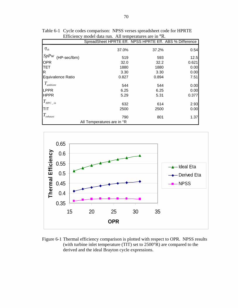
70
Table 6-1 Cycle codes comparison: NPSS verses spreadsheet code for HPRTE Efficiency model data run. All temperatures are in °R.
SpreadSheet HPRTE Eff. NPSS HPRTE Eff. ABS % Difference
37.0% 37.2% 0.54
(HP-sec/lbm) 519 593 12.5OPR 32.0 32.2 0.621TET 1880 1880 0.00R 3.30 3.30 0.00Equivalence Ratio 0.827 0.894 7.51
544 544 0.00LPPR 6.25 6.25 0.00HPPR 5.29 5.31 0.377
632 614 2.93TIT 2500 2500 0.00
790 801 1.37All Temperatures are in °R
thη
SpPw
ambientT
inHPCT _
exhaustT
0.35
0.4
0.45
0.5
0.55
0.6
0.65
15 20 25 30 35
OPR
Ther
mal
Effi
cien
cy
Ideal Eta
Derived Eta
NPSS
Figure 6-1 Thermal efficiency comparison is plotted with respect to OPR. NPSS results (with turbine inlet temperature (TIT) set to 2500°R) are compared to the derived and the ideal Brayton cycle expressions.

71
0.3
0.32
0.34
0.36
0.38
7 10 13 16 19 22 25 28 31 34 37
OPR
Ther
mal
Effi
cien
cy
TIT = 2500°RTIT = 2400°RTIT = 2300°RTIT = 2200°R
SCGT
Figure 6-2 Thermal efficiency vs. OPR with sensitivity to TIT
100
120
140
160
180
200
6 8 10 12 14 16 18 20
OPR
Spec
ific
Pow
er (H
P-se
c/lb
m)
TIT = 2500°RTIT = 2400°RTIT = 2300°RTIT = 2200°R
SCGT
Figure 6-3 Specific power vs. OPR with TIT sensitivity

72
0.33
0.34
0.35
0.36
0.37
0.38
0.39
0.4
500 520 540 560 580Ambient Temperature (°R)
Ther
mal
Effi
cien
cy
OPR = 28OPR = 24OPR = 20OPR = 16OPR = 12
SCGT
Figure 6-4 Thermal efficiency vs. ambient temperature with OPR sensitivity
0.90
0.95
1.00
1.05
1.10
4 5 6 7
LPPR
RH
S of
Equ
atio
n 6.
25
Model Data Points
HPRTE Efficiency
Figure 6-5 Demonstrates agreement between NPSS and developed theory that describes the low pressure spool

73
0
1
2
3
4
5
6
7
8
500 520 540 560 580
Ambient Temperature (°R)
HPP
R
LPPR = 6.4LPPR = 6.0LPPR = 5.5LPPR = 5.0LPPR = 4.5
HPRTE Efficiency
Figure 6-6 High pressure spool pressure ratio (HPPR) vs. ambient temperature with low pressure spool pressure ratio (LPPR) sensitivity
0.33
0.335
0.34
0.345
0.35
0.355
0.36
0.365
0.37
0.375
3 3.5 4 4.5 5 5.5 6 6.5 7 7.5 8
HPPR
Ther
mal
Effi
cien
cy TIT = 2500°RTIT = 2450°RTIT = 2400°RTIT = 2350°R
HPRTE Efficiency
Figure 6-7 Thermal efficiency vs. HPPR showing sensitivity to TIT
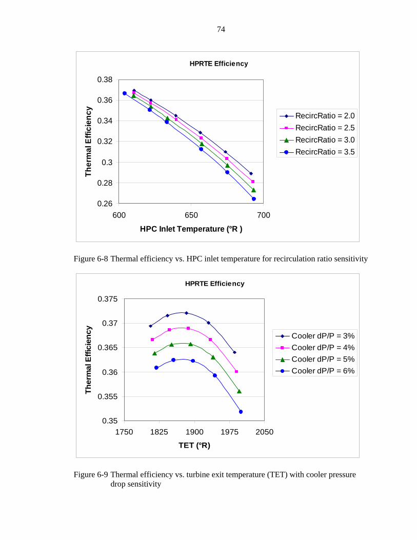
74
0.26
0.28
0.3
0.32
0.34
0.36
0.38
600 650 700
HPC Inlet Temperature (°R )
Ther
mal
Effi
cien
cy RecircRatio = 2.0RecircRatio = 2.5RecircRatio = 3.0RecircRatio = 3.5
HPRTE Efficiency
Figure 6-8 Thermal efficiency vs. HPC inlet temperature for recirculation ratio sensitivity
0.35
0.355
0.36
0.365
0.37
0.375
1750 1825 1900 1975 2050
TET (°R)
Ther
mal
Effi
cien
cy Cooler dP/P = 3%Cooler dP/P = 4%Cooler dP/P = 5%Cooler dP/P = 6%
HPRTE Efficiency
Figure 6-9 Thermal efficiency vs. turbine exit temperature (TET) with cooler pressure drop sensitivity

75
380
420
460
500
540
580
620
1750 1825 1900 1975 2050
TET (°R)
Spec
ific
Pow
er (H
P-se
c/lb
m)
HPC_eff = 0.86HPC_eff = 0.85HPC_eff = 0.84HPC_eff = 0.83
HPRTE Efficiency
Figure 6-10 Specific power vs. TET for HPC efficiency sensitivity
425
475
525
575
625
3 4 5 6 7 8
HPPR
Spec
ific
Pow
er (H
P-se
c/lb
m)
HPT_eff = 0.88HPT_eff = 0.87HPT_eff = 0.86HPT_eff = 0.85
HPRTE Efficiency
Figure 6-11 Specific power vs. HPPR for HPT efficiency sensitivity

76
800
802
804
806
808
810
812
17 22 27 32 37
OPR
Exha
ust T
empe
ratu
re (°
R)
TIT = 2350°R
TIT = 2400°R
TIT = 2450°R
TIT = 2500°R
HPRTE Efficiency
Figure 6-12 Exhaust temperature vs. OPR for TIT sensitivity
0.335
0.34
0.345
0.35
0.355
0.36
0.365
0.37
0.375
2.5 4.5 6.5 8.5
HPPR
Ther
mal
Eff
icie
ncy
Turbo Eff = 0.7138Turbo Eff = 0.6970Turbo Eff = 0.6804
HPRTE Efficiency
Figure 6-13 Thermal efficiency vs. HPPR for turbocharger efficiency sensitivity

77
0.33
0.34
0.35
0.36
0.37
0.38
4 4.5 5 5.5 6 6.5 7 7.5
LPPR
Ther
mal
Eff
icie
ncy
TIT = 2500°RTIT = 2450°RTIT = 2400°RTIT = 2350°R
HPRTE Efficiency
Figure 6-14 Thermal efficiency vs. LPPR for TIT sensitivity
Table 6-2 Summary of the HPRTE Efficiency sensitivity analysis
Perturbed Parameter Specific Power HPPR
TIT 2 1 3
TET 3 1
1
1 1
1 1
1 1
3 1
HPPR 3 2
LPPR 3 1
OPR 3
R 3 2
Cooler 3 3
Resultant Parameter
PΔ
ambientT
inHPCT _
adComp _η
adTurb _η
Turboη
thη exhaustT

78
Table 6-3 Comparison of the thermal efficiency maximums and their corresponding overall pressure ratios (OPRs)
ConfigurationOPR
H-V Eff. 45.0% 23.6 0.442HPRTE Eff. 37.2 32.2 0.368
SCGT 37.3 24.0 0.361SCGT SpPw 33.4 10.4
Parameter
max_thη meanth _η
0.3
0.32
0.34
0.36
0.38
0.4
0.42
0.44
0.46
5 10 15 20 25 30 35 40 45 50
OPR
Ther
mal
Eff
icie
ncy
H-V Eff.HPRTE Eff.SCGT
Figure 6-15 Engine cycles comparison of thermal efficiency vs. OPR
Table 6-4 Comparison of the specific power maximum values and their corresponding OPRs
ConfigurationOPR
H-V Eff. 665 35.0 586HPRTE Eff. 624 42.6 565
SCGT 180 10.5 155
Parameter
SpPw units are industry standard (HP-sec/lbm)
maxSpPw meanSpPw

79
100
200
300
400
500
600
700
5 10 15 20 25 30 35 40 45
OPR
Spec
ific
Pow
er (H
P-se
c/lb
m)
H-V Eff.HPRTE Eff.SCGT
Figure 6-16 Engine cycles comparison of specific power vs. OPR
Table 6-5 Comparison of exhaust temperature maximum values for the three engine configurations
Configuration OPR
H-V Eff. 855 49.0 832HPRTE Eff. 805 42.6 799
SCGT 1660 8.00 1360
Parameter
Temperatures have units of °R
max_exhaustT meanexhaustT _

80
600
800
1000
1200
1400
1600
1800
5 10 15 20 25 30 35 40 45 50
OPR
Exha
ust T
empe
ratu
re (°
R)
SCGTH-V Eff.HPRTE Eff.
Figure 6-17 Engine cycles comparison of exhaust temperature vs. OPR
0.34
0.36
0.38
0.4
0.42
0.44
0.46
500 520 540 560 580 600
Ambient Temperature (°R )
Ther
mal
Effi
cien
cy
H-V Eff.HPRTE Eff.SCGT
Figure 6-18 Engine cycles comparison of thermal efficiency vs. ambient temperature

81
Table 6-6 Engine cycles comparison for four extreme operating conditions
Case SpPw OPR SpPw OPR SpPw OPR1 489°R 544°R 0.397 411 10.2 0.341 390 17.8 0.401 191 24.02 489 499 0.409 436 10.8 0.386 512 23.7 0.401 191 24.03 569 544 0.442 659 30.7 0.367 588 42.0 0.358 144 24.04 569 499 0.444 670 32.3 0.385 675 55.4 0.358 144 24.0
Operating Point H-V Efficiency HPRTE Efficiency SCGTEngine Type
All Specific Power calculations have industry standard units of HP-sec/lbm
thη thη thηambientT waterT
Table 6-7 High pressure compressor (HPC) inlet temperature comparison for the H-V Efficiency engine model
Design Point Parameter 509°R 499°R
45.0% 45.7%
(HP-sec/lbm) 629 639OPR 23.6 22.3TET 1768 1769R 3.00 3.00Equivalence Ratio 0.799 0.799
(lbm/sec) 6.36 6.26
(lbm/sec) 0.306 0.306
545 545LPPR 3.5 3.32HPPR 7.37 7.35
509 499TIT 2500 2500
837 835Temperatures are in °R
airm&
liquidOHm _2&
thη
SpPw
ambientT
inHPCT _
exhaustT
inHPCT _
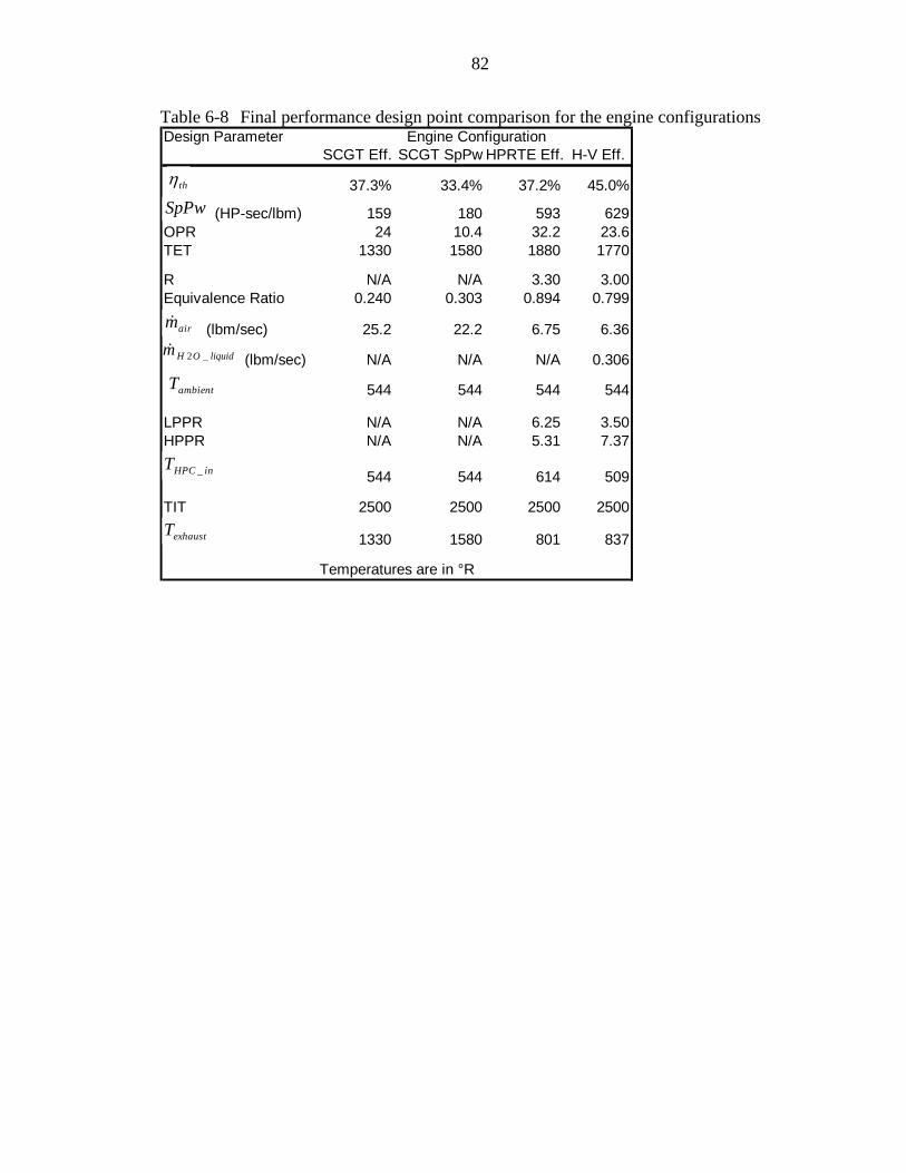
82
Table 6-8 Final performance design point comparison for the engine configurations Design Parameter
SCGT Eff. SCGT SpPw HPRTE Eff. H-V Eff.
37.3% 33.4% 37.2% 45.0%
(HP-sec/lbm) 159 180 593 629OPR 24 10.4 32.2 23.6TET 1330 1580 1880 1770
R N/A N/A 3.30 3.00Equivalence Ratio 0.240 0.303 0.894 0.799
(lbm/sec) 25.2 22.2 6.75 6.36
(lbm/sec) N/A N/A N/A 0.306
544 544 544 544
LPPR N/A N/A 6.25 3.50HPPR N/A N/A 5.31 7.37
544 544 614 509
TIT 2500 2500 2500 2500
1330 1580 801 837
Temperatures are in °R
Engine Configuration
airm&
liquidOHm _2&
thη
SpPw
ambientT
inHPCT _
exhaustT

83
CHAPTER 7 CONCLUSIONS AND RECOMMENDATIONS
Conclusions
The analysis performed for this thesis project consisted of parametric studies to
establish design point parameters, sensitivity studies to examine specific
parameter/resultant interactions, and design point comparisons of the performance
characteristics of the three gas turbine engine configurations. The engine models were
developed using a steady-state, incompressible thermodynamic approach with the engine
cycle code NPSS developed by NASA Glenn Research Center. The mission requirement
for the engine was produce continuous nominal power output of 4000 BHP. To refrain
from investing capital in exotic material development for the engine components, the TIT
maximum was limited to 2500°R and the hot side recuperator inlet temperature was
constrained to not exceed 2059°R. The turbocharger pressure ratio was designed to not
exceed a value of 7.5—this was a design limitation determined for single-stage
centrifugal compressors. Moreover, NPSS and CEA do not have thermodynamic
properties for solids; therefore, to prevent icing before the in the HPRTE engines, the
high pressure compressor (HPC) inlet temperature minimum value was 492°R (33°F).
The dependent variables optimized during the parametric performance comparison of the
engine cycles are listed in their order of significance: thη , specific power, and exhaust gas
temperature.

84
The conclusions are as follows:
• Comparison output from a NPSS run case of the HPRTE Efficiency matched well with output from a similarly configured engine cycle using the spreadsheet code. Those parameters whose values from NPSS agreed with the counterpart values from the spreadsheet code included: thη , OPR, TET, inHPCT _ , and exhaustT . The specific power outputs from the two codes did not match well. Their values differed by 12.5%. The difference in these output values can be associated to three causes. The operational handling of the spreadsheet code was such that it was impossible to model the HPRTE in the proper turbocharger configuration. Moreover, the codes modeled the engine using different fuels and thermodynamic curve-fit equations.
• For the SCGT sensitivity analysis, the results showed that the cycle thermal efficiency and specific power were both particularly sensitive to TIT and ambientT variations but were not very sensitive to OPR changes. This is not surprising when considering the dominance of the temperature ratio in the development of the theoretical thermal efficiency expression in the first section in Chapter 6. The three most noteworthy influence coefficients from this section are
( )36.3
)(=
∂
∂
base
base
TITTIT
SpPwSpPw
( )76.1
)(−=
∂
∂
base
base
TambTamb
SpPwSpPw
( )898.0
)(_ =
∂
∂
base
baseth
th
TITTIT
ηη
.
• Two design points were considered for the SCGT engine configuration. One was optimized for maximum thη (SCGT Efficiency ) and the other was optimized for maximum specific power (SCGT SpPw). The SCGT SpPw best predicts the ETF-40B design point. The SCGT Efficiency had a predicted thη value of 37.3%—10.2% higher than the thη predicted for the SCGT SpPw engine configuration. The SCGT SpPw had a predicted specific power of 180 HP-sec/lbm—13.2% greater than the SCGT Efficiency configuration.
• HPRTE Efficiency sensitivity analysis was performed next. Variations in the following parameters affected the thη resultant by a proportional amount: inHPCT _ ,
adTurb _η , adComp _η , and TIT to a lesser extent. Specific power was decidedly sensitive to these input parameters: TIT, TET, inHPCT _ , adTurb _η , adComp _η , and
Turboη . The HPPR was sensitive to the following parameter inputs: ambientT and LPPR.

85
• A byproduct of the sensitivity analysis for the HPRTE Efficiency was that the optimized pressure ratios for the two spools were determined. The optimization was based on maximizing thη rather than specific power. The turbocharger pressure ratio was chosen to 6.25, and the HPPR was chosen to be 5.31.
• Exhaust gas temperature ( exhaustT ) was an important consideration in the engine cycles comparison studies. exhaustT values for the HPRTE cycles were an average of 550°R less than the exhaustT values of the SCGT Efficiency design point. When compared to the SCGT SpPw design point, the exhaustT values for the HPRTE cycles were almost 800°R less. Cooler exhaust temperatures directly impact the survivability of the ship. Naval ships powered by HPRTE engines instead of SCGT engines would have a greatly reduced infrared detection signature. Moreover, an 800°R reduction in temperature would increase the density of the exhausted gases implying that the exhaust ducting would be smaller in diameter for the HPRTE system.
• The thη values for both HPRTE cycles remain consistently high through a wide operating range of pressure ratio designs. The meanth _η for H-V Efficiency is 44.2% and for HPRTE Efficiency it is 36.8%. The meanth _η of the SCGT was 36.1%. The HPRTE cycle curves for this part of the analysis were very flat meaning that the
thη value is not greatly affected by OPR variations. The implication here is that existing turbomachinery components could most likely be used to design a production HPRTE system.
• The four extreme operating cases analyze the performance characteristics of the competing engine cycles head-to-head. Many conclusions can be drawn from this section of work. First, the H-V Efficiency has better thermal performance in hot weather than in cold weather. Second, thermal performance of the H-V Efficiency is not significantly affected by water temperature. Third, raising air temperature positively impacts the thermal performance and specific power of both HPRTE cycles while negatively affecting both performance characteristics of the open cycle SCGT. Under hot conditions (cases 3 and 4) the H-V Efficiency performed with an average thermal efficiency of 44.3%. That is an average of 17.8% higher than the HPRTE Efficiency cycle and 23.7% higher than the SCGT.
• The effects of decreasing HPC inlet temperature on a H-V Efficiency configured engine were analyzed. The data reveals that there are minor increases (less than 2%) in the performance variables thη and specific power when HPC inlet temperature is dropped from 509°R to 499°R; however, those increases are not significant enough to make a recommendation for this concept.
• For their optimized design point parameters, the H-V Efficiency has a thη of 45.0%—besting the SCGT Efficiency by 20.6%, the SCGT SpPw cycle version by

86
34.7%, and the HPRTE Efficiency engine cycle by 21.0%. Thermal efficiency is inversely related to the specific fuel consumption. For the same ship platform, the H-V Efficiency engines would allow for increased cargo if the mission range is unchanged. The HPRTE cycles should also be considered if the important design issue is mission range. Having lower specific fuel consumption than the SCGT SpPw design point suggests that the HPRTE cycles would exhibit an increased mission range capability if the fuel tank size is a constant parameter.
• There are significant specific power differences between the HPRTE engine cycles and the SCGT. The mean specific power of the H-V Efficiency cycle is nearly four times larger than that of the SCGT. Since specific power is directly proportional to the area of the ducting in the engine, the core HPRTE engine would be almost four times smaller than a SCGT of the same power capacity (of course some additional space would be needed to house the VARS unit). Currently, it is unknown if the size and performance trade-offs would cancel each other.
Recommendations
• An off-design point analysis should be completed on the engine cycle configurations reported on in this analysis because over 93% of naval ship operation time is spent operating at or below 35% engine power [Landon]. NPSS would be the obvious software choice for this next step since it has off-design point modeling capabilities. Moreover, the engine models have already been created in NPSS and the output has been benchmarked to a certain degree. Performance map integration and scaling is a critical competency that must be addressed before this next step is taken; and it is unknown how the performance map look-ups would affect model computing times. Of course, any added sophistication to a model increases the expectation that it will lengthen the model run-time. Currently, for the H-V Efficiency model, the run-times range from 4 to 12 minutes, depending on the model its constraints. A comprehensive off-design study should include range and propeller analysis, as well.
• Further benchmarking of the results of this analysis is a necessary next step to guarantee the accuracy of the work. The accuracy of NPSS is not in question; it was developed by NASA in conjunction with leading United States aero-propulsion companies. However, checking the fidelity of the HPRTE models against other thermodynamic cycle codes, such as the code created by Jameel Kahn, is a useful next step to give confidence to this work. Furthermore, comparing NPSS model results against experimental test data from the laboratory demonstrator should be considered.
• A more robust model would include the VARS unit, at least to the extent that the HPC inlet temperature is set by calculations representative of having the VARS unit in the model. Thus far, excess cooling capacity of the VARS has not been addressed, but there are obvious uses for additional refrigeration on a naval ship.

87
• Other software modeling programs should be considered for future performance analysis of the power and refrigeration cycles being examined by the University of Florida (UF). One commercial software package currently being explored by the Energy and Gas Dynamics Laboratory at UF is ASPEN Plus. ASPEN Plus is an industry leader in process flow modeling and has proven capabilities modeling gas turbine power and refrigeration cycles. Not only can it model design point performance, but off-design analysis is available.
• There are other HPRTE layout designs being explored by UF. Even the current test rig in the Energy and Gas Dynamics Laboratory has a slightly different gas flow path than the HPRTEs in this analysis. Instead of introducing the fresh air before the evaporator, the current test engine rig has the air inlet ducted into the entrance to generator heat exchanger of the VARS unit.
• Since the analysis was done assuming dry ambient air, perhaps more cases should be run on the H-V Efficiency to determine how the added moisture of humid air would affect the water extraction rate.
• A variant design of the H-V Efficiency cycle would have a lower nominal power output rating. Then, during the infrequent instances of operation that full power (4000 BHP) is needed, the water being extracted after the evaporator could be re-injected downstream of the HPC exit to provide the needed boost in horsepower.

88
LIST OF REFERENCES
[1] About Inc., “The History of Engines-How Engines Work Part 2: A Short History and Timeline of Gas Turbine Engines,” The New York Time Company, [online], http://inventors.about.com/library/inventors/blenginegasturbine.htm, [retrieved 18 December 2006].
[2] Shaw, R. J., “A Short History of Turbine Engines,” Ultra-Efficient Engine
Technology Program, NASA, John H. Glenn Research Center at Lewis Field, Cleveland, OH, http://www.ueet.nasa.gov/engines101.php#history, [retrieved 18 December 2006].
[3] Mattingly, J. D., Elements of Gas Turbine Propulsion, McGraw Hill, Inc., New York,
1996, pp. 232-233. [4] Brady, C.O., & Luck, D.L., “The Increased Use of Gas Turbines as Commercial
Marine Engines,” Journal of Engineering for Gas Turbines & Power, ASME, April 1994, pp. 428-433.
[5] Harmon, R., “Marine Gas Turbine: A New Generation,” Mechanical Engineering,
May 1990, pp. 48-51. [6] Davis, R. C., “Final Test Report of Wolverine Gas Turbine Plant,” Research and
Development Report #030076 Ns-6220210, U.S. Naval Engineering Experiment Station, Annapolis, 14 August 1956.
[7] GE Aviation, “The History of Aircraft Engine,” General Electric Company, [online],
http://www.geae.com/aboutgeae/history.html, [retrieved 18 December 2006]. [8] Valenti, M., “Propelling Jet Turbines to New Uses,” Mechanical Engineering, March
1993, pp. 68-72. [9] Ness, J.C., Franks, C.B., Sadala, R.L., “Economic Considerations for a New Gas
Turbine System in the U. S. Navy,” Journal of Engineering for Gas Turbines & Power, ASME, April 1988, pp. 271-272.
[10] GE Infrastructure Marine, “Making Waves: The Rugged, Reliable 7FDM Diesel
Engine,” The General Electric Company, [online brochure], http://www.mshs.com/pdf/GE7FDMBrochure.pdf, [retrieved 18 December 2006].
89
[11] Vericor, “TF Series Marine Gas Turbine Engines – 4000 to 5000 Hp,” MTU Aero Engines Company, [online brochure], p http://www.vericor.com/products/downloads/Marine_tfseries_datasheet.pdf, [retrieved 18 December 2006].
[12] MacFarlane, R.S., Lear, W.E., “System Impact of H2O Production and Injection of a
Novel Semi-Closed Cycle Gas Turbine,” AIAA, 35th Aerospace Sciences Meeting and Expo, Reno, NV, USA, Jan. 1997.
[13] Landon, J.C., “Design and Off-Design Point Study of Two Regenerative Feedback
Turbine Engines for Marine Applications,” Master’s Thesis, University of Florida, Gainesville, Dept. of Mechanical Engineering, 1996.
[14] “Fuel-Saving Warship Drives,” Mechanical Engineering Magazine Online, Aug.
1998: n. page, Online, ASME, 5 Aug. 2006. [15] Korakianitis, T., Beler, K.J., “Investigation of the Part-Load Performance of Two
1.12 MW Regenerative Marine Gas Turbines,” ASME, Journal of Engineering for Gas Turbines & Power, April 1994, pp. 418-423.
[16] Gasparovic, N., “The Advantage of Semi-Closed Cycle Gas Turbines for Naval Ship
Propulsion,” Naval Engineers Journal, April 1968, pp. 275-281. [17] GSP Team, “GSP-Gas turbine Simulation Program,” National Aerospace
Laboratory—The Netherlands, [online], http://www.gspteam.com/main/main.shtml, [retrieved 18 December 2006].
[18] Danias, G.A., “Design and Off-Design Point Study of Two Regenerative Feedback
Turbine Engines for Marine Applications,” Master’s Thesis, University of Florida, Gainesville, Dept. of Mechanical Engineering, 1997.
[19] “Aspen Plus”, Aspen Technology, Inc., [online] July 2006,
http://www.aspentech.com/brochures/aspenplus.pdf, [retrieved 18 December 2006].
[20] United States, NASA, John H. Glenn Research Center at Lewis Field, NPSS User
Guide, Cleveland, OH, 2006. [21] Nemec, T., Lear, W. E., “Thermodynamic Performance of a Semi-Closed Gas
Turbine Combined with a Rankine Bottoming Cycle,” AIAA, 36th Aerospace Sciences Meeting and Expo, Reno, NV, USA, Jan. 1998.
[22] Boza, J. J., 2003, “Performance of a Novel Semi-Closed Gas Turbine Refrigeration
Combined Cycle,” ASME, Turbo Expo: Power for Land, Sea, & Air, Atlanta, GA, USA, June 2003.

90
[23] Malhatra, V., “Life-Cycle Cost Analysis of a Novel Cooling and Power Gas Turbine Engine,” Master’s Thesis, University of Florida, Gainesville, Dept. of Mechanical and Aerospace Engineering, 2005.
[24] Khan, J., Lear, W., Sherif, S., “Performance of a Novel Combined Cooling and
Power Gas Turbine with Water Harvesting,” ASME, Turbo Expo: Power for Land, Sea, & Air, Vienna, Austria, April 2004.
[25] Gordon, S., and McBride, B. J., ( 1994, October), “Computer Program for
Calculation of Complex Chemical Equilibrium Compositions and Applications,” Cleveland, OH, NASA Reference Publication 1311.
[26] Hill, P., and Peterson, C., Mechanics and Thermodynamics of Propulsion, Addison-
Wesley Publishing Company, Reading, MA, 1992, pp. 173. [27] Turns, S. R., An Introduction to Combustion: Concepts and Applications, McGraw-
Hill Book Company, Boston, MA, 2000.

91
BIOGRAPHICAL SKETCH
The author is a native of Flagler Beach, Florida. He earned a bachelor of science
degree in aerospace engineering from the University of Florida in 2004. For the past 2 ½
years he has been a member of the Energy and Gas Dynamics Laboratory at the
University of Florida. His graduate emphasis was firmly focused in the thermal sciences
with selective coursework including gas turbine propulsion systems, combustion, and
entrepreneurship for engineers. His future plans include working in nuclear power
generation in Crystal River, FL.