1

OPTIMIZATION OF COPPER FUNGICIDE APPLICATION TIMING FOR CITRUS GROVES IN FLORIDA

By

TIAGO ZORTEA

A THESIS PRESENTED TO THE GRADUATE SCHOOL

OF THE UNIVERSITY OF FLORIDA IN PARTIAL FULFILLMENT OF THE REQUIREMENTS FOR THE DEGREE OF

MASTER OF SCIENCE

UNIVERSITY OF FLORIDA

2013

2

© 2013 Tiago Zortea

3

To my family and everyone else who have helped me be the better person I am today

4

ACKNOWLEDGMENTS

I am immensely grateful to my advisor Dr. Clyde Fraisse along with Dr.

Willingthon Pavan for providing me the opportunity to study in the United States, which

greatly broadened my perspectives. Dr. Fraisse performed well beyond his expected

duties as advisor by having an intense care for the well-being of me and other students

advised by him. I also give thanks to the other committee members, Dr. Senthold

Asseng, Dr. Douglas D. Dankel and especially to Dr. Megan Dewdney who considerably

helped in improving this study.

I owe my dearest thanks to my mom for being a model of perseverance and

pursuit to improvement in my life. Without her, I would not be able to withstand the long

journey and all the failures that inevitably happen in life. I thank my dad for our endless

analytical conversations about the most varied topics; these conversations are for sure

the very reason why I am so interested in science, which defines me today.

I also thank my girlfriend, Jennifer Grace and my sisters, Laisa and Cindi Zortea

for bringing so much joy and support to my life. I extend my gratitude to Leonilce Girardi

for greatly improving me as a person. Finally I would like to thank my fellow graduate

students for their assistance and encouragement and the Citrus Initiative for funding this

project.

5

TABLE OF CONTENTS

page

ACKNOWLEDGMENTS .................................................................................................. 4

LIST OF TABLES ............................................................................................................ 7

LIST OF FIGURES .......................................................................................................... 8

ABSTRACT ................................................................................................................... 10

CHAPTER

1 INTRODUCTION .................................................................................................... 12

Objective ................................................................................................................. 14 Citrus Production in Florida ..................................................................................... 15

The Copper Residue Model .................................................................................... 16 Disease Management Models for Citrus ................................................................. 17 AgroClimate ............................................................................................................ 18

Summary ................................................................................................................ 19

2 SYSTEM DEVELOPMENT AND SIMULATION METHODS ................................... 20

Understanding the Copper Model Java Source Code ............................................. 20

Web-based Interface Development on AgroClimate ............................................... 23

Analysis of the Copper Residue Using Historical Data ........................................... 26 Meteorological Data ......................................................................................... 26 Analysis of Fruit Protection Based on the Traditional 21-Day Schedule ........... 28

Analysis of Fruit Protection Based on the Web Tool Recommendations .......... 29 Sensitivity Analysis of The Model to Application Parameters ........................... 29

Copper Application Schedule Optimization ............................................................. 30 Optimization of Fruit Protection Using a Varying Interval Schedule ................. 31 Optimization of Fruit Protection Using a Varying Concentration Schedule ....... 33

Summary ................................................................................................................ 35

3 RESULTS AND DISCUSSION ............................................................................... 36

Web-tool ................................................................................................................. 36 Model Evaluation .............................................................................................. 38

Sensitivity Analysis ........................................................................................... 42 System Evaluation ............................................................................................ 44 Web-tool Usage Statistics ................................................................................ 46

Dynamic Optimized Schedules ............................................................................... 50

4 CONCLUSIONS ..................................................................................................... 54

6

APPENDIX

COPPER RESIDUE MODEL TRANSLATED TO R ...................................................... 56

LIST OF REFERENCES ............................................................................................... 61

BIOGRAPHICAL SKETCH ............................................................................................ 64

7

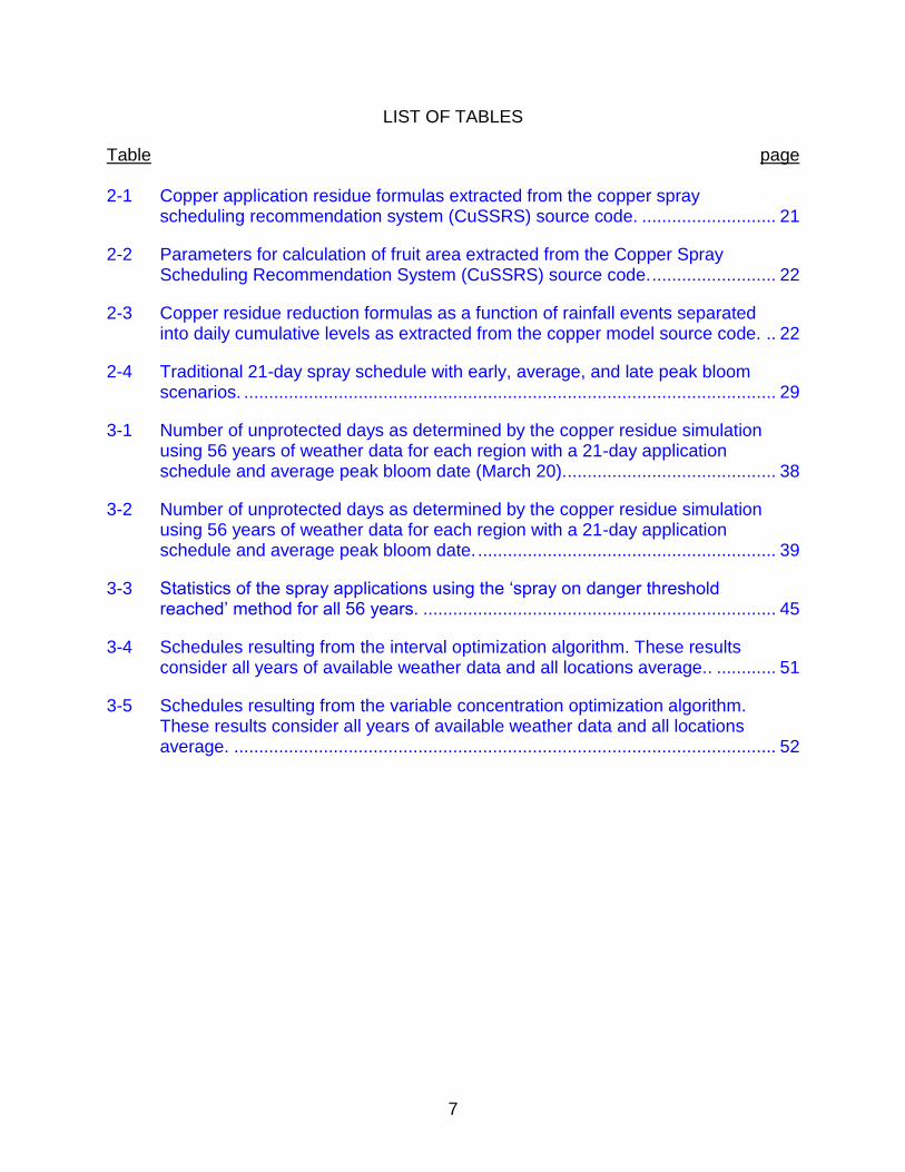
LIST OF TABLES

Table page 2-1 Copper application residue formulas extracted from the copper spray

scheduling recommendation system (CuSSRS) source code. ........................... 21

2-2 Parameters for calculation of fruit area extracted from the Copper Spray Scheduling Recommendation System (CuSSRS) source code. ......................... 22

2-3 Copper residue reduction formulas as a function of rainfall events separated into daily cumulative levels as extracted from the copper model source code. .. 22

2-4 Traditional 21-day spray schedule with early, average, and late peak bloom scenarios. ........................................................................................................... 29

3-1 Number of unprotected days as determined by the copper residue simulation using 56 years of weather data for each region with a 21-day application schedule and average peak bloom date (March 20). .......................................... 38

3-2 Number of unprotected days as determined by the copper residue simulation using 56 years of weather data for each region with a 21-day application schedule and average peak bloom date. ............................................................ 39

3-3 Statistics of the spray applications using the ‘spray on danger threshold reached’ method for all 56 years. ....................................................................... 45

3-4 Schedules resulting from the interval optimization algorithm. These results consider all years of available weather data and all locations average.. ............ 51

3-5 Schedules resulting from the variable concentration optimization algorithm. These results consider all years of available weather data and all locations average. ............................................................................................................. 52

8

LIST OF FIGURES

Figure page 1-1 Florida citrus production by county in 2009-10 according to the Florida

Department of Agriculture and Consumer Services (FDACS, 2011). ................. 16

2-1 Simulation steps of the copper spray scheduling recommendation system (CuSSRS) showing the daily loop required to estimate daily copper residue levels. ................................................................................................................. 20

2-2 Components diagram of a copper residue simulation on the developed web tool. ..................................................................................................................... 25

2-3 Selected National Weather Service (NWS) Cooperative Observer Program (COOP) stations for historical data analysis in Florida. ...................................... 27

2-4 Steps of the program created to analyze combinations of different intervals between each copper application. ...................................................................... 33

2-5 Steps of the program created to analyze combinations of different concentrations on each copper application. ....................................................... 34

3-1 The citrus copper application scheduler on the AgroClimate website (July, 2012). ................................................................................................................. 37

3-2 Copper residue simulation for Hendry County in 2008 using the 21-day schedule and typical spray parameters. The crosses are residue on grapefruit and dots are residue on mandarins.. .................................................. 40

3-3 Comparison between the 21-day spray schedule (A) and the ‘spray when danger threshold reached (in red)’ method (B).. ................................................. 41

3-4 Number of unprotected days summed across 56 years of every weather station. Each data point shows the simulated results varying only the spray volume from 467 to 4676 L ha-1.. ........................................................................ 43

3-5 Number of unprotected days summed across 56 years of every weather station. Each data point shows the simulated results varying only the spray concentration from 0.56 to 4.48 kg ha-1 by increments of 0.056 kg ha-1. ............ 44

3-6 Copper residue simulation using worst-case scenario plant parameters, mandarin fruit inside the canopy, 0.84 kg ha-1 metallic copper concentration, 1170 L ha-1 volume, and Polk County weather data of 2005. ............................. 46

3-7 Map of Florida showing number of unique visitors of the Copper web-tool produced using Google Analytics™. The visitors are grouped by metropolitan areas. ................................................................................................................. 47

9

3-8 Plot of a Gaussian kernel density estimate of the 1460 bloom dates recorded by the web-tool. The vertical line marks March 20th which is the suggested average bloom date. ........................................................................................... 48

3-9 Plot of a Gaussian kernel density estimate of 3259 spray volumes recorded by the web-tool. The vertical line marks 1170 L ha-1 (125 gal ac-1) concentration which is the current recommendation. .......................................... 49

3-10 Plot of a Gaussian kernel density estimate of 3259 spray concentrations recorded by the web-tool. The vertical line marks 0.84 kg ha-1 (0.75 lb ac-1) concentration which is the current recommendation. .......................................... 50

3-11 Plot the average unprotected days of each schedule produced by both interval optimization (continuous line) and concentration optimization (dashed line) for the average bloom date scenario. ......................................................... 53

10

Abstract of Thesis Presented to the Graduate School of the University of Florida in Partial Fulfillment of the Requirements for the Degree of Master of Science

OPTIMIZATION OF COPPER FUNGICIDE APPLICATION TIMING FOR CITRUS

GROVES IN FLORIDA

By

Tiago Zortea

December 2013

Chair: Clyde William Fraisse Major: Agricultural and Biological Engineering

Copper fungicides are commonly used for protective applications against foliar

fungal and bacterial diseases in citrus groves. Management of these products must be

finely balanced between disease prevention, application costs, fruit blemishes caused

by copper phytotoxicity, and toxic accumulation of copper in the soil. The traditional

schedule for copper sprays in Florida is an every 21-day post-bloom application.

However, our computer simulation analysis showed that this traditional schedule is

inefficient; it leaves the grove unprotected in wet years and applies unnecessary copper

sprays in dry years. In order to facilitate the copper management for citrus growers, a

user-friendly internet-based decision support system was developed. This system is

capable of estimating the copper residue on the fruit based on rainfall records and spray

details. This information allows producers to plan the copper applications in order to

minimize unprotected periods while avoiding unnecessary applications in dry years. For

growers who are distant from weather stations or that cannot quickly adjust their

schedules according to the web tool recommendations, we developed a schedule with

varying application intervals or spray concentrations. These schedules were calculated

11

with the objective of minimizing the number of unprotected days according to historic

weather data.

12

CHAPTER 1 INTRODUCTION

Copper (Cu) compounds are the most widely used fungicides or bactericides in

Florida citrus for the management of foliar diseases (Albrigo et al., 2005; Graham et al.,

2010; Graham et al., 2011). Traditionally, copper fungicides have been used to manage

diseases such as melanose (caused by Diaporthe citri), Alternaria brown spot (caused

by Alternaria alternata), citrus scab (caused by Elsinoë fawcettii) and greasy spot rind

blotch (caused by Mycosphaerella citri) (Dewdney et al., 2012a). Particularly for

melanose, sufficient copper residue must be present to protect fruit from petal fall until

mid-July, when the fruits are no longer susceptible to these diseases (Albrigo et al.,

2005). More recently, two new diseases were introduced to Florida; Asian citrus canker,

caused by the bacterium Xanthomonas citri subsp. citri and citrus black spot, caused by

the fungus Guignardia citricarpa (Spann, T.M., 2008; Schubert et al., 2012). Copper

applications are an essential part of the management programs for these diseases

(Schutte et al., 1997; Graham et al., 2010; Graham et al., 2011; Dewdney et al., 2012a;

Dewdney et al., 2012b). However, citrus is susceptible to black spot and citrus canker

until September and October, respectively, and not much is known about how copper

residue decay is affected by the high summer rainfall common in Florida.

Copper, as any agricultural input, has to be correctly dimensioned. If the

concentration of copper is too high, it can frequently cause or accentuate market-value

reducing blemishes due to copper stippling (phytotoxic burn) from excessive copper ion

uptake by the fruit rind cells, especially at temperatures above 34.5°C (Schutte et al.,

1997; Timmer and Zitko, 1998). Furthermore, toxic levels of copper can build-up in soil

due to multiple, high concentration applications of copper over many years (Alva et al.,

13

1993; Graham et al., 1986). In older groves where copper has been used for many

years, the soil can contain up to 370 kg ha-1 metallic copper (Timmer and Zitko, 1996).

High copper concentrations in the soil can slow growth, thin canopies, darken fibrous

roots and cause foliar iron deficiency, particularly on acid soils (Alva et al., 1993;

Graham et al., 1986). Historically, it was recommended to use one or two applications of

9 kg ha-1 metallic copper for foliar disease management (Timmer and Zitko, 1996). It

was shown that lower rates of copper fungicides could give the same disease

management efficacy as the higher rates (Timmer et al., 1998) and that splitting the

applications, without increasing the total copper used per year improved disease

management (Timmer and Zitko, 1998). These findings and other studies were used to

better understand the behavior of copper as a fungicide or bactericide in Florida citrus

groves (Albrigo et al., 1997; Timmer and Zitko, 1996; Timmer et al., 1998) and to

develop a copper spray scheduling recommendation system (CuSSRS) (Albrigo et al.,

2005) to aid growers in scheduling copper fungicide sprays for early season disease

management.

The CuSSRS was evaluated by comparing predicted residue levels to actual

copper residue levels in the field. Disease severity in plots sprayed following the

CuSSRS predictions were compared with a standard 21-day calendar schedule and an

unsprayed treatment (Albrigo et al., 2005). The traditional 21-day schedule is the

currently recommended application schedule (Dewdney and Graham, 2012) and is

commonly used by Florida citrus growers, especially for melanose and/or canker

management. Although the CuSSRS was shown to effectively reduce cost and improve

coverage (Albrigo et al., 2005), it was not widely used by citrus growers. The reasons

14

given by growers for not adopting the system included a confusing interface, too many

inputs, difficult to install, unclear output and lack of updates. A problem in the routine

which connected to the Florida Automated Weather Network (FAWN;

http://fawn.ifas.ufl.edu/) for real time weather information across the state was another

problem that made the copper system difficult to use. To revive this valuable tool, a

project was initiated to develop a web-based version of CuSSRS with a simple and self-

explanatory interface to allow growers to estimate copper residue in their groves and

analyze the results without external aid. The connection between weather data and

disease models is an essential step in order to enhance the contribution of these

models to the producers (Guillespie and Sentelhas, 2008).

Objective

Our primary objective was to help Florida citrus growers better schedule copper

applications and maximize fruit protection while reducing environmental impacts and

production costs. This objective has to be fulfilled with a practical interface aiming to

require the least possible time commitment from the producer.

Specific objectives included:

To understand and review the algorithms used in the CuSSRS model and the sensitivity of the model to the various inputs.

To translate the original CuSSRS model to the R statistical language (R Development Core Team, 2011).

To analyze the variability of copper residue coverage using historical meteorological data for citrus producing areas in Florida and current schedule recommendations.

Develop a practical web tool which allows producers to simulate the remaining copper residue with minimal effort.

To analyze the potential benefits of the developed web tool based on simulations.

15

Develop optimizations for the current recommendations using historical weather data.

Citrus Production in Florida

Citrus production is important to the Florida economy. During the 2010-2011

season, Florida produced more than 63% of United States citrus in a combined area of

203,799 ha for all types (USDA, 2011). Approximately 84% of the Florida citrus

production is processed for juice. The estimated production value of Florida Citrus in the

2010-2011 season was US$ 1,573,116,000 which represents 52% of total citrus

production value from United States (USDA, 2011). Florida Citrus production is

principally located in central and southwestern Florida. Florida citrus growers in 2009-

2010 produced 133.7 million boxes (40.8 kg box-1) of sweet oranges, 96% being used

for juice and 20.3 million boxes (38.5 kg box-1) of grapefruit of which 54% were used for

grapefruit juice. Other citrus types grown in Florida include specialty fruit like mandarin

(tangerine) hybrids and Navel orange. The specialty fruit industry is concentrated on the

Central Ridge of Florida in Lake, Orange and Polk Counties and many grapefruit

plantings are on the East coast in Indian River and St. Lucie Counties (Fig. 1-1).

16

Figure 1-1. Florida citrus production by county in 2009-10 according to the Florida

Department of Agriculture and Consumer Services (FDACS, 2011).

The Copper Residue Model

The CuSSRS model was created to simulate the copper residue decay on citrus

fruit over time. It was developed with the Java programming language as a stand-alone

application and integrated within a larger citrus planning and scheduling program called

DISC (Decision Information System for Citrus) (Beck, 2006). The residual copper is

calculated on a daily basis from the most recent application relying on inputted spray

details and daily rainfall.

The required input information includes bloom date, cultivar, details on copper

spray applications such as concentration and spray volume, fruit position, and daily

17

rainfall data. The different copper concentrations and volumes produce dissimilar

residue levels on the fruit. Fruit growth and rainfall events are used to simulate the

amount of copper residue decreased by fruit surface expansion and weathering of the

residue layer. The model simulates the copper residue for fruit located inside and

outside of the tree canopy. The copper deposition and rainfall events affect the outer

fruit more intensely than the inner fruit (Albrigo et al., 2005). Interior fruit and fruit on the

top of the tree receive lower copper deposits from commonly used spray equipment. On

the other hand, there is less rainfall removal of copper for interior fruit or less disease

pressure for the top of the tree when considering melanose (Albrigo et al., 2005). Very

low spray diluent volumes can lead to excessive deposits on exterior surfaces of outer

fruit which can cause copper stippling in addition to poor disease management on

interior fruit (Albrigo et al., 1997). Increasing diluent rate produced a more uniform

coverage along the tree but also increased the copper lost by run-off (Albrigo et al.,

1997).

The copper residue threshold for reapplication was based on the recommended

values needed to provide a complete protection safety margin. CuSSRS adopts a

default warning threshold of 0.5 µg cm-2 and a danger threshold of 0.25 µg cm-2. The

minimum residue in which the grove is still considered protected is 0.1 µg cm-2 (Albrigo

et al., 2005).

Disease Management Models for Citrus

Other systems have been proposed to help citrus growers better manage

diseases. The ALTER-RATER is a weather-based model with the objective of help

producers correctly time fungicide sprays for Alternaria management (Bhatia, A.,

2002;Timmer et al., 2001). It is based on a cumulative score, which is influenced by

18

rainfall, leaf wetness and temperature. The system does not have a web interface and

requires the producer to manually fill the weather data in a table. Also a model was

developed for management of Post bloom fruit drop, caused by Colletotrichum acutatum

(Timmer et al., 1996). This model has shown to produce accurate predictions but

requires considerably more information beyond weather data.

AgroClimate

AgroClimate is a web-based climate information and decision support system

(http://www.agroclimate.org) (Fraisse et al., 2006) developed to help agricultural

producers reduce risks associated with climate variability in the southeastern U.S.A.

(Fraisse et al., 2006). It is periodically updated and maintained to ensure up-to-date

information and the simplest possible interface. A mobile version is also available when

the AgroClimate website is accessed from a mobile device. It was designed and

implemented by the Southeast Climate Consortium (SECC-http://seclimate.org) in

partnership with the Florida Cooperative State Extension Service. The system was

developed to be hosted in Linux/Unix platforms but can easily be transferred to others.

The dynamic tools were developed using the PHP (Hypertext Preprocessor) web

programming language, Javascript language, HTML, Cascading Style Sheets (CSS)

and MySQL database (Pavan et al., 2011).

Decision support tools available in AgroClimate include: (a) Climate risk tools:

expected (probabilistic) and historical climate information as well as freeze risk at the

county level; (b) Crop yield tools: expected yield based on soil type, planting date, and

basic management practices for corn, cotton, peanut, potato, and tomato, and historical

county and regional yield databases; (c) Crop disease tools: disease risk monitoring and

forecasting for anthracnose and botrytis fruit rot in strawberry, peanut leaf spot, and the

19

citrus copper application scheduler; (d) Crop development tools: monitoring and

forecasting of growing degree-days and chill accumulation; (e) Drought monitoring tools:

monitoring and forecasting of the Agricultural Reference Index for Drought (ARID),

Keetch-Byram (KBDI), and the Lawn and Garden (LGMI) drought indices; and (f)

Footprint tools: carbon footprint of selected fruits and water footprint of cereal crops.

AgroClimate provides climate forecasts and outlooks, monthly climate summaries, crop

management options to mitigate climate-associated risks for pasture, forestry as well as

certain crops and fruits. It also includes background information about the main drivers

of climate variability and basic information about climate change in the Southeast USA.

Summary

This chapter described the objectives of this study and introduced background

information about the citrus production in Florida. Traditional copper management

practices and the copper model used in the simulations contained in this study were

also introduced. Chapter 2 details the copper model inner equations and the methods

used for the simulations. Also in Chapter 2, it is described the development process of

the proposed web tool for copper residue management. Simulation results and the

copper residue web-based tool are discussed in Chapter 3. Chapter 4 includes our main

conclusions and recommendations for future developments.

20

CHAPTER 2

SYSTEM DEVELOPMENT AND SIMULATION METHODS

Understanding the Copper Model Java Source Code

Figure 2-1 shows that the first step in the extracted copper residue model was

the calculation of the copper deposition provided by the first spray application. The

copper residue is always zero at the beginning of the season because the previous

season’s fruit have been harvested by time of application in the spring. The applied

copper residue depends on the fruit area available, volume and concentration of the

copper suspension, and the position of the fruit, inside or outside the tree canopy

(Table 2-1).

Figure 2-1. Simulation steps of the copper spray scheduling recommendation system

(CuSSRS) showing the daily loop required to estimate daily copper residue levels.

21

Table 2-1. Copper application residue formulas extracted from the copper spray scheduling recommendation system (CuSSRS) source code.

Fruit position Volume (L ha-1) Formula to estimate copper residue[a]

Inside <1,169

Inside >=1,169 and <=2,338

Inside 2,338

Outside <1,169

Outside >=1,169 and <=2,338

Outside >2,338

[a]The volume (V) is in L ha-1 and concentration (C) is in kg ha-1. Area on the day of application (A) is

provided by

A Gompertz growth function using the parameters described in Table 2-1 was

used to estimate fruit growth. Because it is an empirical approximation, the model does

not use weather data to provide a more precise estimation of fruit area. An idealized

growth curve for each scion is given by Equation 2-1 using the variables and

parameters found in Table 2-2.

The idealized growth curve is calculated as follows:

(2-1)

where AREA is fruit surface area in mm2, T is the sum of the current Julian day with the

regression offset, MAX is the maximum measured AREA, MIN is an arbitrarily small

value and B is the parameter for each scion type (Table 2-2).

22

Table 2-2. Parameters for calculation of fruit area extracted from the Copper Spray Scheduling Recommendation System (CuSSRS) source code.

Cultivar Regression offset (Julian Day)

MAX (mm2) MIN (mm2) B (unitless)

Grapefruit 73 22,650 645 X 10-12 0.0220 ‘Valencia’ 69 14,949 645 X 10-12 0.0222 Mandarin 77 14,263 645 X 10-12 0.0198 ‘Navel’ 64 19,856 645 X 10-12 0.0214

Each day post application, the residue is reduced proportionally to the fruit surface area.

The copper residue in μg cm-2 of a given day is calculated as follows:

(2-2)

Where DEPO is the initial residue from the most recent application and AREA is the

current day’s fruit surface area and calculated by Equation 2-1.

Rainfall events are responsible for rapid copper residue loss. The loss is

proportional to the rainfall amount on a given day and the remaining residue. Table 2-3

shows how rainfall intensities have different effects on residue loss. The residue also

slowly decreases over time because of the increase in the AREA value in Equation 2-2

while DEPO remains constant over time until there is a new application.

Table 2-3. Copper residue reduction formulas as a function of rainfall events separated

into daily cumulative levels as extracted from the copper model source code.

Rainfall (mm) Reduction[a]

> 0 and <= 127

> 127 and <= 508

> 508

[a]Where R is daily rainfall in millimeters and RESIDUE is calculated by

.

Residue thresholds can be adjusted by the user in the CuSSRS model. For this

study a residue threshold of 0.25 µg cm-2 was used as the ‘danger’ threshold. According

to Albrigo et al. (2005), at the 0.25 µg cm-2 ‘danger’ threshold fruit still has complete

23

protection. However an application is advised as soon as the ‘danger’ threshold is

reached since a strong weathering event could leave the grove unprotected. When the

residue falls under 0.1 µg cm-2 a grove is considered unprotected as the remaining

residue is not sufficient to keep the fruit protected (Albrigo et al. 1997; 2005).

Web-based Interface Development on AgroClimate

The copper residue model was extracted from the CuSSRS Java source code

and translated into the R language with the objective of facilitating the production of high

quality graphs, its integration into the AgroClimate web server, and the execution of

statistical analysis. The R statistical analysis software system (http://www.r-project.org)

is a language and environment for statistical computing and graphics generation. It is an

open-source implementation of the S language developed at Bell Laboratories by John

Chambers and colleagues (R Development Core Team, 2011). R is multiplatform, which

means that it can be run on all modern operating systems such as UNIX, Linux,

Windows, and Macintosh. Being able to run under Linux is an important feature when

integrating code with websites as the majority of web servers operate in Linux. R also

provides a well-developed programming language and a self-contained environment to

perform a wide range of statistical analyses. As a programming language, R is highly

expansible allowing it to be easily adapted to new tasks that are not part of the built-in

functionality (R Development Core Team, 2011).

Along with correcting the communication issues that prevented the CuSSRS to

retrieve real-time weather data, the Citrus Copper Application Scheduler was intended

to have a more functional and easier to understand interface, consequently broadening

its use by citrus producers. With daily copper residue information, it is possible for

growers to better time application decisions and reduce the number of unprotected

24

periods. Lapses in residue protection can allow fruit infection to occur by plant

pathogens decreasing their market value.

The tool was designed to be as simple as possible using only free and open

source components following the AgroClimate website guidelines. The website runs in

PHP, HTML (Hyper Text Markup Language), CSS (Cascading Style Sheets) and

JavaScript using the jQuery framework (http://jquery.com/). Since it is available at a

central server, it is possible to deliver updates and corrections with minimal delay.

The model and plots run in the R language. The inputs are stored in a MySQL

(http://www.mysql.com/) database. To further assist decision-making, the tool is linked

to the Citrus Pesticide Application Tool (http://fawn.ifas.ufl.edu/tools/pesticide/) available

on FAWN that provides rainfall forecasts and application conditions for the next 45

hours.

Figure 2-2 shows a diagram of the different components of the copper residue

simulation web tool. The simulation starts with the grower providing spray and grove

information (Fig. 2-2A) on the PHP form. The user provided information is stored in the

MySQL database (Fig. 2-2B) by the PHP algorithm, which also generates a system call

to the R program containing the simulation (Fig. 2-2C). The simulation information is

then retrieved by the R program from the database (Fig. 2-2D), which afterwards

generates a HTTP call (Fig. 2-2E) to the FAWN web service retrieving (Fig. 2-2F)

information from the weather station selected by the user. The copper residue

simulation is then executed based on the information retrieved. The resulting graph is

saved as an image in a specific folder on the server (Fig. 2-2H), the numeric results are

saved back on the database (Fig. 2-2G). After the simulation is finished the PHP code

25

which was halted by the system call continues to run (Fig. 2-2I), it reads the results as

well as the location of the graph on the server (Fig. 2-2J-K) and presents the simulation

information to the user (Fig. 2-2M).

Figure 2-2. Components diagram of a copper residue simulation on the developed web tool.

All the experiments executed by the growers in the website stay anonymously

logged in the database. Additionally, the Google Analytics™ tool was installed in the

website. This tool allows tracking of the website traffic and users behavior. Using the

logged information it was possible to create plots of the average bloom date, average

concentration, and average volume inputted in the website. It was also used to generate

a map of the number of user accesses to the website from Florida. This map was

grouped by a political division called metropolitan area. These divisions are related to

26

densely populated areas which share the same infrastructure, it might encompass

several counties.

Analysis of the Copper Residue Using Historical Data

Having the Copper residue model translated to R enables the possibility of

simulating scenarios using the historical meteorological data. These scenarios can

produce valuable information regarding how different application approaches affected

the copper residue in past years. More specifically, it is possible to count the number of

days in which the grove was unprotected, the number of sprays necessary to achieve

optimal protection, the effect of each model parameter in the results, and how different

rainfall patterns affect the copper residue. It is also possible to test if the current spray

recommendations provided adequate amounts of copper residue through the whole

vulnerability period in different locations.

Meteorological Data

Daily precipitation data are a key input for the copper model as rainfall

significantly reduces current residue levels on the fruit. In this study, two different

meteorological data sources were used. The website tool uses observed data from

FAWN weather stations located in citrus producing areas of the state. FAWN data were

used for in-season simulation of copper residue levels and application scheduling.

Historical analysis of copper application regimens needed a longer time series of daily

weather data than the ones available from FAWN stations. For that reason, fifty-six

years of historical daily weather data from the National Weather Service (NWS)

Cooperative Observer Program (COOP) were used

(http://www.nws.noaa.gov/om/coop). Five locations in the Florida counties of Highlands,

Hendry, Lake, Indian River, and Polk were selected for the historical analysis aiming for

27

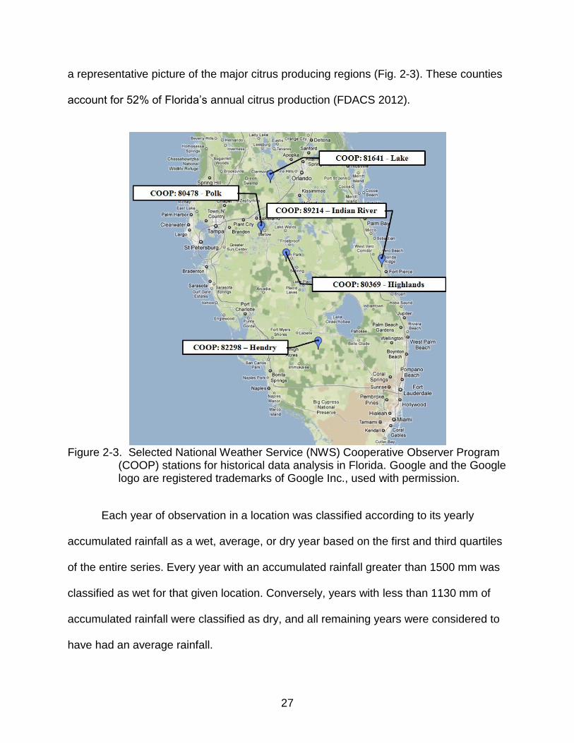
a representative picture of the major citrus producing regions (Fig. 2-3). These counties

account for 52% of Florida’s annual citrus production (FDACS 2012).

Figure 2-3. Selected National Weather Service (NWS) Cooperative Observer Program (COOP) stations for historical data analysis in Florida. Google and the Google logo are registered trademarks of Google Inc., used with permission.

Each year of observation in a location was classified according to its yearly

accumulated rainfall as a wet, average, or dry year based on the first and third quartiles

of the entire series. Every year with an accumulated rainfall greater than 1500 mm was

classified as wet for that given location. Conversely, years with less than 1130 mm of

accumulated rainfall were classified as dry, and all remaining years were considered to

have had an average rainfall.

28

Analysis of Fruit Protection Based on the Traditional 21-Day Schedule

Several simulation experiments were conducted using the copper residue model

and observed weather data to better understand the dynamics of copper residue decay

and how different parameters affect copper residue levels. It was important to determine

which combination of fruit position and scion defined the worst-case scenario. These

parameters have a small but noticeable effect on the copper residue and knowing the

worst-case scenario allowed the simulations to be restricted by assuming that other

scenarios would have superior protection. The criteria used to determine the worst-case

scenario was the number of unprotected days (residue < 0.1 µg cm-2) for different

scions and fruit positions using the traditional 21-day application schedule. This

approach slightly reduced the precision of the analysis but greatly simplified the results

by avoiding the need for different recommendation combinations for each fruit position

and scion.

The simulation experiments produced in this study used the typical spray

parameters for Florida: 0.84 kg ha-1 (0.75 lb ac-1) metallic copper concentration and

1170 L ha-1 (125 gal ac-1) volume (Dewdney et al., 2012a). The period in which the

residue level was evaluated for unprotected days extended from the first spray 3 weeks

post-bloom to the last day of July. The data for CuSSRS stopped in early July because

the fruit are no longer susceptible to melanose (Albrigo et al. 2005), the main disease of

concern prior to citrus canker and black spot.

For simulation standardization, three different peak bloom date scenarios were

used to simulate early, average, and late bloom (Table 2-4).

29

Table 2-4. Traditional 21-day spray schedule with early, average, and late peak bloom scenarios.

Event Early bloom Average bloom Late bloom[a]

Bloom date 10-Mar. 20-Mar. 30-Mar.

1st spray 31-Mar. 10-Apr. 20-Apr.

1st scheduled spray 21-Apr. 1-May 11-May

2nd scheduled spray 12-May 22-May 1-June

3rd scheduled spray 2-June 12-June 22-June

4th scheduled spray 23-June 3-July 13-July

5th scheduled spray 14-July 24-July N/A

End of vulnerability period 31-July 31-July 31-July [a] N/A not applicable

Analysis of Fruit Protection Based on the Web Tool Recommendations

An R program was developed to compare the amount of copper used by the

traditional 21-day copper schedule and the hypothetical case in which producers are

able to spray whenever necessary (copper residue under 0.25 µg cm-2) according to the

citrus copper application scheduler recommendations. For this comparison we used an

average bloom period, copper concentration of 0.84 kg ha-1, spray volume of 1170 L ha-

1, the mandarin scion, and 56 years of rainfall data for all the studied locations. The

objective of the comparison was to measure how many copper applications would be

necessary per year to achieve no unprotected days assuming that the web-tool

recommendations were followed to the letter. Additionally, the difference in residue

levels between dry, average and wet years were calculated.

Sensitivity Analysis of The Model to Application Parameters

Aside from application dates, the spray concentration and volume are the only

parameters that can be easily changed by the producer to achieve better protection.

Although recommendations for these parameters already exist (Dewdney et al., 2012a),

it was important to understand the model sensitivity to them. The model was run by

varying both metallic copper concentration and diluent volume one at a time, small

30

increments, while all other parameters were kept the same. This approach is known as

‘vary one parameter at a time’ sensitivity analysis. Many other more complex sensitivity

analysis approaches have been proposed. These more complex approaches better

cover the search space as in the Morris method (Morris et al., 1991) or use variance

decomposition as in the FAST method (Schaibly et al., 1973) but these are better suited

for large models with unpredictable interactions between the inputs.

For the ‘vary one parameter at a time’ approach, it is necessary to define the

range in which the parameters can vary. The spray volume range was varied from 467

to 4676 L ha-1 by increments of 9.3 L ha-1 and the concentration range was varied from

0.56 to 4.48 kg ha-1 by increments of 0.056 kg ha-1. These are the maximum and

minimum values that were used by producers on the web-tool. It was also necessary to

define the default values for the other model parameters while only one is varied in each

simulation. The typical 21-day spray schedule, average bloom date, inside canopy fruit

position, copper concentration of 0.84 kg ha-1, spray volume of 1170 L ha-1, the

mandarin scion, and 56 years of rainfall data were used for all the studied locations.

This sensitivity analysis approach also required relevant output to be selected.

The sum of the number of unprotected days from the first spray to the end of July

across all years of weather data and locations was selected.

Copper Application Schedule Optimization

Disease control is not always satisfactory with the traditional 21-day schedule

and many Florida citrus farms encompass thousands of hectares or are scattered over

wide areas. In these cases, it is not always possible to quickly move equipment

according to output from a daily model and a compromise was sought to improve the

copper coverage over the traditional schedule for these operations on a set schedule. It

31

was hypothesized that historical weather data along with the fruit growth and copper

residue decay estimates from the CuSSRS could be used to develop a dynamic copper

application schedule with fewer coverage gaps to improve disease management in the

spring and early summer.

Considering that each location had slightly different historical rainfall pattern, a

more optimized schedule for each independent region would exist. This region specific

optimization would produce better results than one optimized for all the regions.

However, there would be a total of 15 optimized schedules, one for each region and

bloom date. It was decided not to publish these results as they were overly complicated

for the producers and the additional protection benefit small.

Optimization of Fruit Protection Using a Varying Interval Schedule

Based on initial observations from the model output, it was determined that the

driving factors behind copper residue loss, fruit growth and rainfall, vary throughout the

growing season. It was then possible to develop a fixed schedule that adjusted the

interval between sprays during the growing season to account for different growing

conditions and weather patterns that could result in more uniform protection.

To further study this hypothesis, an R schedule optimization algorithm was

developed with the objective of generating and testing different scheduling strategies

aimed at the best protection with model outputs and historical weather data. The

generated schedules were ranked by the resulting fruit protection. More specifically the

fruit protection is given by the sum of unprotected days over every year from 1956 to

2012 across the 5 studied locations. The simulations used the worst-case scenario for

fruit position and scion, typical spray parameters, and the first spray started 21 days

32

after bloom (Fig. 2-4). The number of unprotected days was calculated also for the

traditional 21-day schedule with the same parameters to serve as a baseline scenario.

The number of schedule simulations that could be tested was limited by the

substantial computational processing required for this task. The ideal scenario would be

to vary each date for at least +6 to -6 days, but this approach for a 5-spray date season

would create 371,293 different schedules. Considering it would be necessary to run all

these schedules for each of the 56 years for each of the 5 locations, it would create an

impractical total of over 100 million simulations. A more manageable and sophisticated

approach was to vary each schedule for +2 to -2 days requiring only 3,125 whole year

simulations. Then use this local minima result and re-run it again starting out from the

optimized schedule. This process was repeated each time using the best result from the

previous schedules until the resulting optimum schedule was the same as the starting

schedule provided to the algorithm. It is very likely that the result of this approach is also

the global minima because the best schedules usually are similar. However, it can only

be guaranteed to be the local minima in the last run range.

For example, the first experiment for the early bloom date tested schedules with

spray intervals ranging from (19, 19, 19, 19, 19) to (23, 23, 23, 23, 23). These extreme

schedules were obviously not suitable as the first one would produce a period of low

residue in July and the last one simply has too many days between applications leaving

the grove vulnerable. Among all the possibilities there is likely a more efficient schedule

than the 21-day fixed schedule.

There was little difference between the residual copper losses of the different

scion types which supported the contention that it was acceptable to create the

33

optimized schedules based on the worst-case scenario. With the worst-case scenario

as our test subject, the residue decay predictions for the other scion types are likely to

be conservative. This means that if there is an error in the prediction, it is likely to

encourage an application before needed but not allow a lapse in coverage.

Figure 2-4. Steps of the program created to analyze combinations of different intervals between each copper application.

The proposed approach was not supposed to increase amount of copper applied

compared to the amount that would otherwise be applied with the 21-day schedule. For

this reason in the case of late bloom, only 4 copper applications were simulated, 5

applications would have extended the protection past the vulnerable period (Table 2-4).

Optimization of Fruit Protection Using a Varying Concentration Schedule

It is a common practice of Florida growers to combine several products in the

spraying equipment tank in order to minimize costs. These products also have set

schedules, which might complicate the usage of the proposed varying interval schedule.

34

For these cases, a dynamic schedule was proposed, which varies the concentration of

each application and still has the fixed 21-day schedule. This approach is less effective

because the residue lost per day is proportional to the current residue on the fruit.

Consequently greater concentrations also produce greater loss of residue reducing the

overall possible gain in protection.

Figure 2-5. Steps of the program created to analyze combinations of different concentrations on each copper application.

For the varying concentration schedule it was necessary to also vary the

concentration of the first application, which was fixed in the varying interval schedule.

This approach increased the number of possible schedules by 5 times, however the

number of valid proposed schedules was greatly reduced by the fact that this approach

was not supposed to increase the amount of copper applied, consequently limiting the

valid schedules to only those which fit this criteria. The concentrations were varied by

35

±0.122 kg ha-1 (0.10 lb ac-1) with a range of ±0.224 kg ha-1 (0.20 lb ac-1) in each run of

the optimization algorithm.

Summary

In this chapter, it was presented a detailed description of the copper model which

is used in this study including equations and overall structure. It was also described the

methodologies and parameters used in the simulations for accessing copper protection

performance in past scenarios. Additionally, the approach for optimizing both interval of

application and copper concentration in each application optimizations was described.

In chapter 3, it will be presented optimization results, analysis of the current

recommendations for Florida, and the developed and implemented web-tool for

simulating copper residue levels.

36

CHAPTER 3 RESULTS AND DISCUSSION

Web-tool

The web-based application developed for this study works as a practical interface

for the producer with the citrus copper application scheduler. With the daily residue

information, it is possible for producers to make accurate and timely decisions regarding

copper applications. To operate the system, the user inputs the spray concentration and

volume, scion, bloom date and weather data source (Fig. 3-1). This source can be

either the FAWN weather station closest to the grove or a comma separated value

(CSV) file containing the user’s rain measurements. The ‘Simulate copper residue’

button creates a graph that shows the daily copper residue from 3 days before first

spray until a week after the current day. The blue bars indicate rainfall events and the

red/yellow areas are the danger and warning thresholds respectively. When the residue

reaches the warning level, the grower is advised to plan for an application. When the

residue reaches the danger zone, the grower is advised to make an application as soon

as possible. Additional information about the system’s operation can be found in

(Dewdney et al. 2012a).

37

Figure 3-1. The citrus copper application scheduler on the AgroClimate website (July, 2012).

The user also can see the model results in table format or download them as a

CSV file. A detailed screencast on how to use the website is provided in the link ‘Help

screencast’. Clicking on the corresponding data fields allows the user to change the

default quantity of metallic copper per area and spray volume. To calculate the

kilograms of metallic copper used, it is necessary to multiply the percent metallic copper

in a product (found on the label) by kg ha-1 used. The fruit position is not requested

because it would not make sense to ask that question to a producer; instead the worst-

case scenario is always assumed (fruit inside the canopy).

38

Model Evaluation

Simulation results of the traditional 21-day schedule (Table 3-1) indicate that of

all scion combinations and fruit positions, the fruit inside the canopy of a mandarin type

scion were the least protected with an average of 3.12 unprotected, under 0.1 µg of

copper cm-2 , days per year. This combination of parameters was then considered to be

the worst-case scenario and used in all other simulations in this study.

Table 3-1. Number of unprotected days as determined by the copper residue simulation using 56 years of weather data for each region with a 21-day application schedule and average peak bloom date (March 20).

Florida County Grapefruit Valencia Mandarin

Tot.[a] Max Avg.[a] Tot. Max Avg. Tot. Max Avg.

Fruit inside the canopy

Hendry 257 26 4.59 271 27 4.84 282 27 5.04

Highlands 153 21 2.73 167 21 2.98 171 21 3.05

Indian River 102 13 1.82 116 14 2.07 119 14 2.12

Lake 114 14 2.04 125 15 2.23 138 15 2.46

Polk 153 11 2.73 167 11 2.98 174 11 3.11

Average 156 - 2.78 170 - 3.02 177 - 3.16

Fruit on the canopy surface

Hendry 150 23 2.68 160 23 2.86 166 23 2.96

Highlands 74 12 1.32 78 12 1.39 83 15 1.48

Indian River 49 11 0.88 52 11 0.93 55 11 0.98

Lake 41 10 0.73 49 10 0.88 49 10 0.88

Polk 67 8 1.20 72 8 1.29 71 8 1.27

Average 76 - 1.36 84 - 1.47 85 - 1.51 [a]

Tot. – total Avg. –average per year

Table 3-2 shows the simulated maximum and average unprotected days using

the worst-case scenario parameters for each yearly-accumulated rainfall classification.

The minimum is not displayed because it was 0 for all the proposed scenarios. There is

39

a large difference in the number of unprotected days in wet years compared to dry

years, with more unprotected days occurring in wet years.

Table 3-2. Number of unprotected days as determined by the copper residue simulation

using 56 years of weather data for each region with a 21-day application schedule and average peak bloom date.

Florida County Dry[a] Average[a] Wet[a]

Max Avg./year Max Avg./year Max Avg./year

Hendry 4 1.07 16 5.58 27 7.18

Highlands 7 0.71 13 3.22 21 4.62

Indian River 6 0.81 13 2.18 14 3.46

Lake 8 1.15 11 2.21 15 4.55

Polk 7 1.29 10 2.68 11 5.40

Average - 1.00 - 3.17 - 5.04 [a] Classification based on the first and third quartiles of the yearly accumulated rainfall. Years with accumulated rainfall greater than 1500 mm were classified as wet. Years with accumulated rainfall less than 1130 mm were classified as dry and all remaining years were considered to have had an average rainfall.

Figure 3-2 shows a residue simulation of a typical wet year, 2008, for Hendry

County showing the difference in residue decay between grapefruit and mandarin. In

this scenario, the grove would have been unprotected from June 26th to July 2nd and

from July 15th to the end of the season with the traditional 21-day application schedule.

This was a typical case in which a varied application schedule would have provided

much more efficient protection with the same amount of copper by delaying the first 3

applications. There were little differences between the residual copper decay of the

different scions.

40

Figure 3-2. Copper residue simulation for Hendry County in 2008 using the 21-day schedule and typical spray parameters (0.84 kg ha-1 metallic copper concentration and 1170 L ha-1 volume). The crosses are residue on grapefruit and dots are residue on mandarins. The red threshold is 0.25 µg cm-2 of copper and the black line is 0.1 µg cm-2. The blue bars are daily total rainfall.

In contrast to wet years, a substantial amount of copper is often wasted in dry

years. For example, Figure 3-3 shows the copper residue continuously accumulated

from April to July, 1998. Yet, in July even a small amount of rain washed off most of the

copper residue because the residue loss is proportional to the residue present (Table 2-

1). This is in agreement with the current theory that there is no reason to apply large

amounts of copper in fewer sprays (Timmer et al., 1998). Based on the model, only 3

timed applications were able to keep sufficient copper residue levels thus avoiding 2

unnecessary copper applications (Figure 3-3).

41

Figure 3-3. Comparison between the 21-day spray schedule (A) and the ‘spray when danger threshold reached (in red)’ method (B). These simulations were run using 1998 Lake County weather data for mandarin types and typical spray parameters (0.84 kg ha-1 metallic copper concentration and 1170 L ha-1 volume) and the traditional 21-day schedule. The red threshold is 0.25 µg cm-

2 of copper and the black line is 0.1 µg cm-2.

42

The citrus copper application scheduler can be used to estimate summer copper

residue decay but it may not be as accurate as for early season estimates. The causes

of these potential inaccuracies include the fruit growth curves, which estimate growth

between petal fall and early July, when growth is faster than in the summer. After this

period, our preliminary data showed a slower fruit expansion over the summer and fall.

In addition, rainfall becomes more scattered with thunderstorms and potentially more

intense during the summer compared to spring and early summer. It is not known how

the slowing of fruit growth along with the seasonal change in rainfall patterns can affect

copper residue levels. Summer copper residue predictions will eventually be improved

with data generated by on-going experiments.

Sensitivity Analysis

With the ‘vary one at a time’ sensitivity analysis of the spray volume (Fig. 3-4), it

was possible to demonstrate that different volumes change the number of unprotected

days. The recommended volume of 1170 L ha-1 volume is located exactly on the optimal

protection point.

43

Figure 3-4. Number of unprotected days summed across 56 years of every weather station. Each data point shows the simulated results varying only the spray volume from 467 to 4676 L ha-1 by increments of 9.3 L ha-1. All the other inputs for the model were kept fixed according to the defined worst case scenario. The dashed line shows the current recommendation of 1170 L ha-1 result.

Figure 3-5 shows the ‘vary one at time’ concentration sensitivity analysis. This

parameter had a logarithmic impact on the number of unprotected days. The

recommended concentration of 0.84 kg ha-1 is a well-balanced value between a

reasonable amount of protection and an economical use of copper. It was also shown

that concentrations greater than 1.5 kg ha-1 should be avoided as they provide little

increase in protection while increasing the chance of fruit blemishes caused by copper

phytotoxicity.

44

Figure 3-5. Number of unprotected days summed across 56 years of every weather station. Each data point shows the simulated results varying only the spray concentration from 0.56 to 4.48 kg ha-1 by increments of 0.056 kg ha-1. All the other inputs for the model were kept fixed according to the defined worst case scenario. The dashed line shows the current recommendation of 0.84 kg ha-1 result.

System Evaluation

The citrus copper application scheduler allows citrus producers to achieve

greater precision in the grove’s copper residue. For instance, in some exceptionally dry

years, even with the worst-case scenario of mandarin fruit inside the canopy, only 3

standard copper applications were able to keep the residue levels over the danger

threshold for the entire season (Fig. 3-3) in the simulated scenarios. On the other hand,

Figure 3-6 shows an extreme case of a year with intense rainfalls where seven

applications were necessary to hold the residue always above the danger threshold.

With the traditional 21-day schedule, there would have been several critical gaps in

copper coverage.

45

The same approach of applying copper when the danger threshold is reached

was then simulated for all 56 years of weather data and all stations. These simulations

showed that across all locations in average years it would be necessary to use 6.2

standard copper sprays to keep the residue above the danger zone with the average

bloom scenario. Also, the average period between needed applications was 20.6 days;

this number suggests the current recommended 21-day schedule is a reasonable

average. However, many years are not ‘average’ and there are gaps in coverage or

excess applications for very wet or dry years, respectively (Table 3-3).

Table 3-3. Statistics of the spray applications using the ‘spray on danger threshold reached’ method for all 56 years. Typical spray parameters and average bloom period were used. The worst-case scenario, mandarin fruit inside the canopy, was used as plant parameters.

Florida County

Average number of

applications (wet years)

Average number of

applications (average

years)

Average number of

applications (dry years)

Average number of days between

applications (all years)

Average yearly

rainfall (mm)

(all years)[a]

Hendry 6.4 6.2 5.7 19.2 587

Highlands 6.4 5.9 5.4 20.4 537

Indian River 5.8 5.5 5.0 21.9 444

Lake 6.4 5.9 5.0 21.0 512

Polk 6.3 5.8 5.4 20.5 536 All Counties Averaged 6.2 5.8 5.3 20.6 523

[a] In the considered period, from first spray to 31 July.

46

Figure 3-6. Copper residue simulation using worst-case scenario plant parameters, mandarin fruit inside the canopy, 0.84 kg ha-1 metallic copper concentration, 1170 L ha-1 volume, and Polk County weather data of 2005. The spray schedule used was the ‘spray on danger threshold reached’. The red danger threshold is 0.25 µg cm-2 of copper and the black line is 0.1 µg cm-2.

Web-tool Usage Statistics

Figure 3-7 shows the number of unique visitors from Florida to the created web-

tool. This figure is restricted to only visits incoming from Florida; other areas with

significant number of visits include California, Brazil and China. The central Florida

region had a greater number of visitors, this is an expected result as this area has the

most Citrus production (Figure 1-1). However, the large number of visitors from the

Gainesville area is explained by tests by the staff of University of Florida and is not

representative of the Citrus producers.

47

Figure 3-7. Map of Florida showing number of unique visitors of the Copper web-tool produced using Google Analytics™. The visitors are grouped by metropolitan areas. Google and the Google logo are registered trademarks of Google Inc., used with permission.

Figure 3-8 shows a Gaussian kernel density estimate of the bloom dates

recorded by the web-tool. A peak of bloom dates around mid March can be observed,

this peak is in agreement with proposed bloom dates of the executed experiments

(Table 2-4). The peak in the beginning of the year however is explained by the fact that

the website suggests a valid date up to 21 days before the current date as default value

for bloom date, consequently most of the users visiting the website in January will have

the date automatically set to January 1st increasing the odds of these dates.

48

Figure 3-8. Plot of a Gaussian kernel density estimate of the 1460 bloom dates recorded by the web-tool. The vertical line marks March 20th which is the suggested average bloom date.

Figure 3-9 shows a Gaussian kernel density estimate of 3259 spray volumes

recorded by the web-tool. The peak at 125 gal ac-1 shows that most of producers do not

modify the suggested default value, but there are also noticeable peaks at 200 and 250

gal ac-1. This result suggests that some producers use more diluted spray applications.

49

Figure 3-9. Plot of a Gaussian kernel density estimate of 3259 spray volumes recorded by the web-tool. The vertical line marks 1170 L ha-1 (125 gal ac-1) concentration which is the current recommendation.

Figure 3-10 shows a Gaussian kernel density estimate of 3259 spray

concentrations recorded by the web-tool. The peak at 0.75 lb ac-1 shows that most of

producers do not modify the suggested default value, however there are several high

concentration peaks at 1.5, 2.0 and 3.0 lb ac-1. These results suggest that many

producers still use high concentration applications, which were shown to provide little

increase in protection.

50

Figure 3-10. Plot of a Gaussian kernel density estimate of 3259 spray concentrations recorded by the web-tool. The vertical line marks 0.84 kg ha-1 (0.75 lb ac-1) concentration which is the current recommendation.

It is important to realize that web sites statistics have strong biases towards

default values and towards the region in which the website was produced. This

subsection would have more realistic information if it was possible to exclude all the

traffic incoming from University of Florida and if every field on the web-tool had no

default values. Yet default values are crucial for the web-tool usability and help the

producers to be aware of the recommended parameters.

Dynamic Optimized Schedules

For each peak bloom date scenario, the R schedule interval optimization

algorithm was run until the dates converged to a point at which no better schedule was

found. On average, 3 executions of the optimizing algorithm were needed. Table 3-4

shows the result of each algorithm execution. It is important to remember that each

51

peak bloom date scenario has its own schedule. Consequently for scions with large

differences in the peak bloom date or different vulnerability period, these schedules

should be modified to reflect the new conditions. The reduction column of Table 3-4

refers to the reduction in the number of unprotected days when compared to the usual

21-day interval schedule. The average number of unprotected days per year/station

using the 21-day interval schedule for early, average and late bloom were respectively

2.38, 3.10 and 3.78.

Table 3.4 Schedules resulting from the interval optimization algorithm. These results

consider all years of available weather data and all locations average, the worst-case scenario as plant parameters and typical spray volume and concentration.

Peak Bloom Interval to spray[b] Average of unprotected days per year/station

Reduction %[c]

1st 2nd 3rd 4th 5th

Early 20 24 21 19 19 1.9 18.9

Average 19 24 16 17 17 1.5 50.9

Late 22 22 20 19 N/A[a] 3.3 11.7 [a] Not applicable. [b] Number of days after the last spray. The first spray is always 21 days after peak bloom (Table 2-4), the ‘1st’ indicates the interval how many days after the previous spray it was applied. [c] The percent reduction of the mean of unprotected days across all years and stations compared to the 21-day schedule using the traditional spray parameters.

The improved protection given by the optimized schedule is due to a better

distribution of copper applications over time. The average bloom schedule got the

greatest benefit because in the 21-day schedule the last spray (Table 2-4) would

provide most of its protection outside the proposed vulnerability period which extends

until end of July. These results show how a variable interval spray schedule can

increase the fruit protection by distributing the residue more evenly according to the

rainfall pattern and vulnerability pressure.

52

Table 3-5. Schedules resulting from the variable concentration optimization algorithm. These results consider all years of available weather data and all locations average, the worst-case scenario as plant parameters and typical spray volume and concentration and 21-day application schedule.

Peak Bloom

Concentration of spray[b]

Average of unprotected days

per year/station

Reduction %[c]

1st 2nd 3rd 4th 5th 6th

Early 0.75 0.55 0.75 0.95 0.95 0.55 2.1 11.6

Average 0.85 0.55 0.85 0.95 0.75 0.55 2.7 13.6

Late 0.75 0.65 0.85 0.95 0.55 NA[a] 3.5 7.5 [a] Not applicable. [b] Copper concentration of each spray including the first one after peak bloom (Table 2-4). [c] The percent reduction of the mean of unprotected days across all years and stations compared to the 21-day schedule using the traditional spray parameters.

However, it is important to keep in mind that the optimized schedules are an

empirical analysis of the copper residue influenced by past rain distribution.

Consequently, in the majority of years, the optimized schedule will perform better, but

there can be years in which the benefit will be minimal.

53

Figure 3-11. Plot the average unprotected days of each schedule produced by both interval optimization (continuous line) and concentration optimization (dashed line) for the average bloom date scenario. The horizontal line marks the average protection of the traditional approach of 21 days interval and 0.84 kg ha-1 (0.75 lb ac-1) concentration for all copper applications. Each mark in the x-axis corresponds to one simulated optimization.

The concentration optimization has less satisfactory results as shown in Figure 3-

11. Increasing the concentration of the applications has diminishing effects with larger

values consequently reducing the margin for improvement. It is also possible to see how

inadequately planned schedules can greatly decrease the protection. The worst tested

schedules had an increase of more than 100% in the number of unprotected days.

54

CHAPTER 4 CONCLUSIONS

The citrus copper application scheduler, a web-based decision support system,

enables citrus growers to easily access information to make decisions concerning the

timing of copper applications. By using the web-based tool, growers can reduce copper

applications in dry years and minimize unprotected periods in wet years. The results of

the copper model with a threshold of 0.25 µg cm-2 and historical weather data showed

that the traditional 21-day schedule at recommended copper application rates did not

provide enough residual copper to protect groves in wet years. Conversely, it was

shown that it is possible to avoid unnecessary copper applications in dry years by

optimizing the timing of the sprays.

Two approaches for optimizing the copper schedules were proposed with the

objective of evenly distributing the copper protection according to the historic weather

data. The optimized schedule with varying intervals between applications was able to

attain 50% fewer unprotected days for the simulated period using the average bloom

date scenario. The optimized schedules with varying concentrations provide an

alternative for producers, who must have a fixed interval spray schedule, but it provides

smaller gains in protection.

Lastly, this study provides a documentation of the algorithm used in the source

code of the copper model as well as a study of the model sensitivity to change in

parameters. It was found that the current recommendations for spray volume and

concentration are a good tradeoff between protection and amount of copper applied.

As future developments, there exists an ongoing effort for allowing the user to

automatically use the Real-Time Mesoscale Analysis (RTMA, http://www.nco.ncep.noaa

55

.gov/pmb/products/rtma ) rainfall data for a producer’s specific area instead of using

FAWN weather stations. Since RTMA is calculated on a 5-km wide grid, it would likely

have more precise rainfall information when the grove is distant from a weather station.

Also, the fruit growth functions for the model end in early July. With the arrival of citrus

canker and black spot, copper applications are needed throughout the summer. Fruit

growth and copper residue loss data are being gathered. These data will be used to

improve the residue predictions from July to October and be added to the model.

56

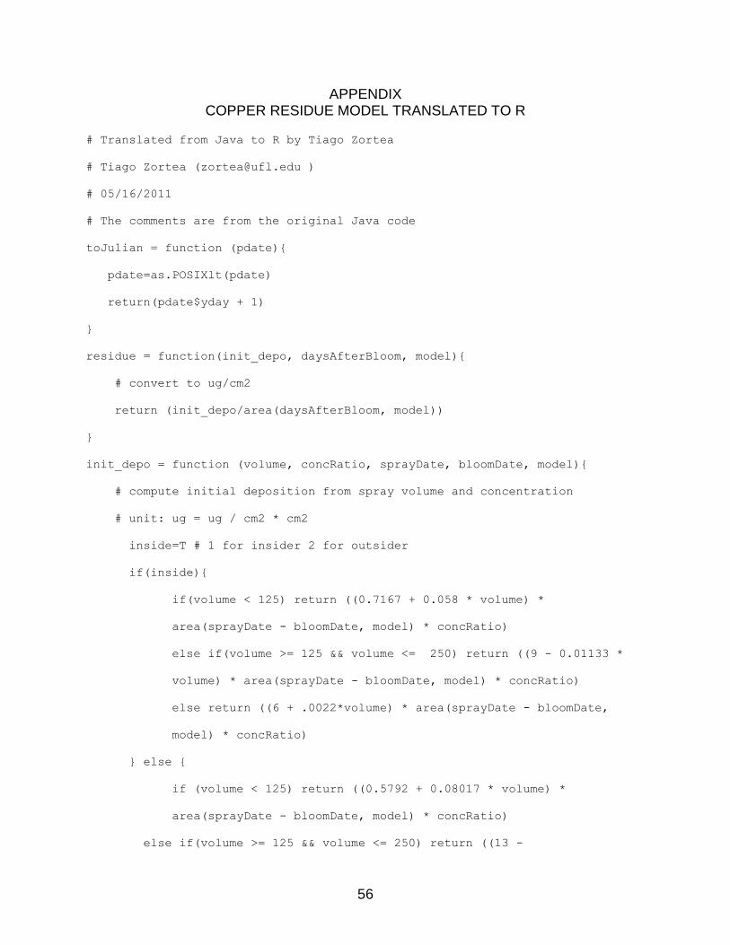
APPENDIX COPPER RESIDUE MODEL TRANSLATED TO R

# Translated from Java to R by Tiago Zortea

# Tiago Zortea (zortea@ufl.edu )

# 05/16/2011

# The comments are from the original Java code

toJulian = function (pdate){

pdate=as.POSIXlt(pdate)

return(pdate$yday + 1)

}

residue = function(init_depo, daysAfterBloom, model){

# convert to ug/cm2

return (init_depo/area(daysAfterBloom, model))

}

init_depo = function (volume, concRatio, sprayDate, bloomDate, model){

# compute initial deposition from spray volume and concentration

# unit: ug = ug / cm2 * cm2

inside=T # 1 for insider 2 for outsider

if(inside){

if(volume < 125) return ((0.7167 + 0.058 * volume) *

area(sprayDate - bloomDate, model) * concRatio)

else if(volume >= 125 && volume <= 250) return ((9 - 0.01133 *

volume) * area(sprayDate - bloomDate, model) * concRatio)

else return ((6 + .0022*volume) * area(sprayDate - bloomDate,

model) * concRatio)

} else {

if (volume < 125) return ((0.5792 + 0.08017 * volume) *

area(sprayDate - bloomDate, model) * concRatio)

else if(volume >= 125 && volume <= 250) return ((13 -

57

0.016 * volume) * area(sprayDate - bloomDate, model) * concRatio)

else return ((11 - .0078 * volume) * area(sprayDate -

bloomDate, model) * concRatio)

}

}

reduceRatio = function(rain){

if (rain >= 0 && rain <= 0.5) return (.48 * rain)

if (rain > 0.5 && rain <= 2) return (.12 * (rain - 0.5) + .24)

return (0.42)

}

area = function (daysAfterBloom, model){

if (tolower(model) == "grapefruit")

return (gompertz(daysAfterBloom,73,22650,0.0220))

if (tolower(model) == "valencia")

return (gompertz(daysAfterBloom,69,14949,0.0222))

if (tolower(model) == "mandarin")

return (gompertz(daysAfterBloom,77,14263,0.0198))

if (tolower(model) == "navel")

return (gompertz(daysAfterBloom,64,19856,0.0214))

#Orange (generic, use valencia parameters)

return (gompertz(daysAfterBloom,69,14949,0.0222))

}

residue = function(init_depo, daysAfterBloom, model){

# convert to ug/cm2

return (init_depo / area(daysAfterBloom, model))

}

gompertz = function (daysAfterBloom, originalBloomDate, max, b){

# Gompertz equation...

# AREA = MAX*EXP(LN(MIN/MAX)*EXP(-B*T))

58

#

# AREA = fruit surface area in square millimeters

# T = date (julian, Jan 1 = 1)

# MIN = Minimum Size (always 0)

# MAX = Maximum Size (estimated for each experiment)

# B = parameter (estimated for each experiment)

# originalBloomDate is date regression was based on

# daysAfterBloom is days since bloom in current year

# add to get adjusted julian date (accounts for the fact

# that bloom date this year might not be same as bloom

# date in original year)

# Max B

#Control Block/Yellow valencia 14949 0.0222

#Shade/Pink valencia 14611 0.0213

#Plastic Block/Pink valencia 14763 0.0215

#Control Block/Yellow grapefruit 22650 0.0220

#Shade/Pink grapefruit 22733 0.0217

#Plastic Block/Pink grapefruit 24116 0.0216

#Fallglo 14263 0.0198

#Navel 19856 0.0214

julianDate = originalBloomDate + daysAfterBloom

min = 0.000000000645 # very small

return (max * exp( log(min / max) * exp(-1 * b * julianDate)))

}

simulateResidue = function(experiment) {

sql = paste ("SELECT simID, CONVERT( scion, CHAR ) as scion ,

bloom_date FROM simCtrl WHERE simID=",experiment)

rs = dbSendQuery(con,statement=sql)

experimentPar = na.omit(fetch(rs,n=-1))

59

experimentPar[,'bloom_date']=toJulian(experimentPar[,'bloom_date'])

sql = paste ("SELECT date , inches FROM simRain WHERE simID=",

experiment," order by date")

rs = dbSendQuery(con,statement=sql)

experimentRain = na.omit(fetch(rs,n=-1))

experimentRain$date=toJulian(experimentRain[,1])

sql = paste ("SELECT date, volume, concentration FROM simSpray

WHERE simID=",experiment," order by date")

rs = dbSendQuery(con,statement=sql)

experimentSprays = na.omit(fetch(rs,n=-1))

experimentSprays$date=toJulian(experimentSprays[,1])

concRatio = experimentSprays[1,'concentration'] / 4

startDate=experimentSprays[1,'date']

scion=experimentPar[1,'scion']

results=rep(0,366)

depo =init_depo(experimentSprays[1,'volume'],concRatio,

startDate,experimentPar[1,'bloom_date'],scion)

results[1]=residue(depo,startDate-experimentPar[1,'bloom_date'],scion)

change=0

for (x in 2:366){

idx=which.max(match(experimentRain$date,startDate + (x - 1)))

if(length(idx)>0){

change = -reduceRatio(experimentRain[idx,'inches']) * depo;

}

idx=which.max(match(experimentSprays$date,startDate + (x - 1)))

if(length(idx)>0){

concRatio = experimentSprays[idx,'concentration'] / 4

change =init_depo(experimentSprays[idx,'volume'],concRatio,

experimentSprays[idx,'date'],

60

experimentPar[1,'bloom_date'],scion)

}

# rainfall occurs, Cu reduced, re-calculate the coefficient of

# the exp function: data=new_co * e ^ (x) (x-starts from zero...)

depo=depo + change

results[x]=residue(depo,startDate + (x -

1) - experimentPar[1,'bloom_date'],scion)

change = 0;

}

return(results)

}

61

LIST OF REFERENCES

Albrigo, L.G., H.W. Beck, L.W. Timmer, and E. Stover. 2005. Development and testing of recommendation system to schedule copper sprays for citrus disease control. Journal of ASTM International 2, 1-12.

Albrigo, L.G., L.W. Timmer, K. Townsend, and H.W. Beck 1997. Copper fungicides - residues for disease control and potential for spray burn. Proceedings of the Florida State Horticultural Society 110, 67-70.

Alva, A.K., J.H. Graham, and D.P.H. Tucker. 1993. Role of calcium in amelioration of copper phytotoxicity for citrus. Soil Science 155, 211-8.

Bhatia, A., P.D. Roberts, and L.W. Timmer. 2003. Evaluation of the Alter-Rater model for timing of fungicide applications for control of Alternaria brown spot of citrus. Plant Dis. 87:1089-1093.

Beck, H.W., L.G. Albrigo, and S. Kim. 2006. DISC citrus planning and scheduling program. Acta Hort. (ISHS) 707, 25-32. Available at http://www.actahort.org/books/707/707_2.htm. Accessed 14 January 2013.

Dewdney, M.M., and J.H. Graham. 2012. Citrus canker. In 2012 Florida Citrus Pest Management Guide, edited by M.E. Rogers, M.M. Dewdney, T.M. Spann, Gainesville, FL: University of Florida, IFAS. pp. 6. Available at http://edis.ifas.ufl.edu/cg040. Accessed 14 January 2013.

Dewdney, M.M., C.W. Fraisse, T. Zortea, and J.D. Burrow. 2012a. A Web-based tool for timing copper applications in Florida citrus. Publ. No. PP289. Univ. Florida, IFAS, EDIS, Gainesville. (4 pp.) Available at http://edis.ifas.ufl.edu/pp289. Accessed 14 January 2013.

Dewdney, M.M., T.S. Schubert, M.R. Estes, and N.A. Peres. 2012b. Citrus black spot. In 2012 Florida Citrus Pest Management Guide, edited by M.E. Rogers, M.M. Dewdney, T.M. Spann, Gainesville, FL: University of Florida, IFAS. pp. 6. Available at http://edis.ifas.ufl.edu/cg088. Accessed 14 January 2013.

FDACS (Florida Department of Agriculture and Consumer Services). 2011. Florida Agriculture By The Numbers 2011. http://www.florida-agriculture.com/pubs/pubform/pdf/florida_agricultural_statistical_directory.pdf

FDACS. 2012. Florida Citrus Statistics 2010-2011. Florida Department of Agriculture and Consumer Services. Available at: http://www.nass.usda.gov/Statistics_by_State/Florida/Publications/Citrus/fcs/2010-11/fcs1011.pdf. Accessed 14 January 2013.

62

Fraisse, C.W., N.E. Breuer, D. Zierden, J.G. Bellow, J. Paz, V.E. Cabrera, A. Garcia y Garcia, K.T. Ingram, U. Hatch, G. Hoogenboom, J.W. Jones, and J.J. O'Brien. 2006. AgClimate: A climate forecast information system for agricultural risk management in the southeastern USA. Computers and Electronics in Agriculture 53, 13-27.

Guillespie, T.J., and P.C. Sentelhas. 2008. Agrometeorology and plant disease management – A happy marriage. Sci. Agric. 65: 71-75.

Graham, J.H., M.M. Dewdney,and M.E. Meyers. 2010. Streptomycin and copper formulations for control of citrus canker on grapefruit. Proceedings of the Florida State Horticultural Society 123, 92-99.

Graham, J.H., M.M. Dewdney, H.D. Yonce. 2011. Comparison of copper formulations for control of citrus canker on ‘Hamlin’ orange. Proceedings of the Florida State Horticultural Society 124, 79-84.

Graham, J.H., L.W. Timmer, and D. Fardelmann. 1986. Toxicity of fungicidal copper in soil to citrus seedlings and vesicular-arbuscular mycorrhizal fungi. Phytopathology 76, 66-70.

Morris, M.D. 1991. Factorial sampling plans for preliminary computational experiments. Technometrics 33, 161-174.

Pavan, W., C.W. Fraisse, and N.A. Peres. 2011. Development of a web-based disease forecasting system for strawberry. Computers and Electronics in Agriculture 75, 169-175.

R Development Core Team. 2011. R: A language and Environment for Statistical Computing. R Foundation for Statistical Computing, Vienna, Austria, ISBN: 3- 900051-07-0. http://www.R-project.org.

Schaibly, J.H., and K.E. Shuler. 1973. Study of the sensitivity of coupled reaction systems to uncertainties in rate coefficients. II Applications. Journal of Chemical Physics, 59, 3879–3888.

Schubert, T.S., M.M. Dewdney, N.A. Peres, M.E. Palm, A. Jeyaprakash, B. Sutton, S.N. Mondal, N.Y. Wang, J. Rascoe, and D.D. Picton, . 2012. First report of Guignardia citricarpa associated with citrus black spot on sweet orange (Citrus sinensis) in North America. Plant Disease 96, 1225.

Schutte, G.C., K.V. Beeton, and J.M. Kotze. 1997. Rind stippling on Valencia oranges by copper fungicides used for control of citrus black spot in South Africa. Plant Disease 81, 851-4.

Spann, T.M., R.A. Atwood, J.D. Yates, R.H. Brlansky, and K.R. Chung, . 2008. Dooryard citrus production: Citrus Diseases Exotic to Florida. Publication No. HS1132, University of Florida, IFAS, EDIS, Gainesville, Florida.

63

Sutton, J.C., T.J. Gillespie, and P.D. Hildebrand. 1984. Monitoring weather factors in relation to plant disease. Plant Dis. 68:78-84.

Timmer, L.W., H. M. Darhower, and A. Bhatia. 2001. The Alter-Rater, a new weather-based model for timing fungicide sprays for alternaria control. Publication No. SP-175, University of Florida, IFAS, EDIS, Gainesville, Florida.

Timmer, L.W., and S.E. Zitko. 1996. Evaluation of a model for prediction of postbloom fruit drop of citrus. Plant Disease. 80:380-383.

Timmer, L.W., and S. E. Zitko. 1996. Evaluation of copper fungicides and rates of metallic copper for control of melanose on grapefruit in Florida. Plant Disease 80, 166-169.

Timmer, L.W., S.E. Zitko, and L.G. Albrigo. 1998. Split applications of copper fungicides improve control of melanose on grapefruit in Florida. Plant Disease 82, 983-6.

USDA. 2011. Citrus Fruits 2011 Summary September 2011. Available at: http://usda01.library.cornell.edu/usda/nass/CitrFrui//2010s/2011/CitrFrui-09-22-2011.pdf . Accessed 14 January 2013.

64

BIOGRAPHICAL SKETCH

Tiago Zortea was born in Passo Fundo, Brazil on October, 1983. He obtained an

Associate’s degree in Electronics from the Cecy Leite Costa Institute along with his high

school degree in 2004. After, he enrolled in the Electrical Engineering program at

University of Passo Fundo, but soon he realized his real passion was in the computing

sciences. In 2005, he changed his major to Computer Science obtaining the degree of

Bachelor’s of Computer Science in 2011. To be able to afford the high educational

costs, he began searching for a job as soon as he began his college studies. Still in

2005, he started working as Assistant Developer at the Caixa Federal Bank. In 2007, he

was hired by Compasso S.A. as a Java web developer. In Compasso he quickly

ascended positions; by 2011 he was a Senior Software Engineer leading a team of

developers. Even though he had a fulfilling job by this time, Tiago wanted to be able to

exercise his scientific knowledge also, for that matter he contacted his advisor Dr.

Willingthon Pavan. His advisor, who had attended University of Florida as a research

scholar, contacted Dr. Clyde Fraisse which ultimately led to a position offer to Tiago as

research scholar at University of Florida. In 2011, Tiago was offered a full assistantship

to pursue his graduate education at the Agricultural and Biological Engineering

Department at University of Florida, under the supervision of Dr. Clyde Fraisse.