AUTOMATIC DISEASE DETECTION IN CITRUS TREES - UFDC Image Array 2
116
EVALUATION OF CLASSIFIERS FOR AUTOMATIC DISEASE DETECTION IN CITRUS LEAVES USING MACHINE VISION By RAJESH PYDIPATI A THESIS PRESENTED TO THE GRADUATE SCHOOL OF THE UNIVERSITY OF FLORIDA IN PARTIAL FULFILLMENT OF THE REQUIREMENTS FOR THE DEGREE OF MASTER OF ENGINEERING UNIVERSITY OF FLORIDA 2004
Transcript of AUTOMATIC DISEASE DETECTION IN CITRUS TREES - UFDC Image Array 2

EVALUATION OF CLASSIFIERS FOR AUTOMATIC DISEASE DETECTION IN
CITRUS LEAVES USING MACHINE VISION
By
RAJESH PYDIPATI
A THESIS PRESENTED TO THE GRADUATE SCHOOL OF THE UNIVERSITY OF FLORIDA IN PARTIAL FULFILLMENT
OF THE REQUIREMENTS FOR THE DEGREE OF MASTER OF ENGINEERING
UNIVERSITY OF FLORIDA
2004

Copyright 2004
by
Rajesh Pydipati

I dedicate this document to my parents and my teacher Dr. Burks for their support and friendship. Without them, this work would not have been possible.

ACKNOWLEDGMENTS
I would like to express my gratitude to my parents for their love and support in all
stages of my life. My sincere thanks go to my professor, friend and guide, Dr. Thomas F.
Burks, whose support and faith in me have always been an inspiration. I would also like
to thank Dr. Wonsuk Lee and Dr. Michael C. Nechyba, who agreed to be on my
committee and gave valuable advice in the completion of this research work. My warm
greetings to all my friends in our research group (Agricultural Robotics and
Mechatronics, ARMg) and the personnel in the Agricultural and Biological Engineering
Department for their friendship. Special thanks go to Ms. Melanie Wilder for proof-
reading this document. I extend my special thanks to the United States Department of
Agriculture (USDA) for providing the necessary funds to carry on this research.
iv

TABLE OF CONTENTS page ACKNOWLEDGMENTS ................................................................................................. iv
LIST OF TABLES............................................................................................................ vii
LIST OF FIGURES ......................................................................................................... viii
ABSTRACT.........................................................................................................................x
CHAPTER 1 INTRODUCTION ........................................................................................................1
Motivation.....................................................................................................................1 Citrus Diseases..............................................................................................................2 Image Processing and Computer Vision Techniques ...................................................5
2 OBJECTIVES...............................................................................................................8
3 LITERATURE REVIEW .............................................................................................9
Object Shape Matching Methods..................................................................................9 Color Based Techniques .............................................................................................10 Reflectance Based Methods........................................................................................12 Texture Based Methods ..............................................................................................13 Experiments Based On Other Methods ......................................................................15
4 FEATURE EXTRACTION........................................................................................21
Texture Analysis.........................................................................................................21 Co-occurrence Matrices.......................................................................................23 Autocorrelation Based Texture Features .............................................................24 Geometrical Methods ..........................................................................................25 Voronoi Tessellation Functions...........................................................................25 Random Field Models .........................................................................................26 Signal Processing Methods..................................................................................26
Color Technology .......................................................................................................26 RGB Space ..........................................................................................................27 HSI Space ............................................................................................................29
v

Co-occurrence Methodology for Texture Analysis ....................................................30 SAS Based Statistical Methods to Reduce Redundancy ............................................36
5 CLASSIFICATION....................................................................................................38
Statistical Classifier Using the Squared Mahalanobis Minimum Distance ................39 Neural Network Based Classifiers..............................................................................41
Considerations on the Implementation of Back Propagation ..............................57 Radial Functions..................................................................................................59 Radial Basis Function Networks .........................................................................60
6 MATERIALS AND METHODS ...............................................................................64
SAS Analysis ..............................................................................................................72 Input Data Preparation................................................................................................74 Classification Using Squared Mahalanobis Distance .................................................74 Classification Using Neural Network Based on Back Propagation Algorithm:.........75 Classification Using Neural Network Based on Radial Basis Functions: ..................78
7 RESULTS...................................................................................................................81
Generalized Square Distance Classifier from SAS ....................................................81 Statistical Classifier Based on Mahalanobis Minimum Distance Principle ...............82 Neural Network Classifier Based on Feed Forward Back Propagation Algorithm....82 Neural Network Classifier Based on Radial Basis Functions ....................................83
8 SUMMARY AND CONCLUSIONS........................................................................88
APPENDIX A MATLAB CODE FILES............................................................................................90
B MINIMIZATION OF COST FUNCTION.................................................................96
LIST OF REFERENCES.................................................................................................102
BIOGRAPHICAL SKETCH ...........................................................................................105
vi
LIST OF TABLES
Table page 6-1 Classification models ...............................................................................................73
7-1 Percentage classification results of the test data set from SAS................................81
7-2 Percentage classification results for mahalanobis distance classifier ......................82
7-3 Percentage classification results for neural network using back propagation..........82
7-4 Percentage classification results for neural network using RBF..............................83
7-5 Classification results per class for neural network with back propagation ..............86
7-6 Comparison of various classifiers for model 1B......................................................87
vii

LIST OF FIGURES
Figure page 1-1 Image of citrus leaf infected with greasy spot disease ...............................................3
1-2 Image of a citrus leaf infected with melanose............................................................4
1-3 Image of a citrus leaf infected with scab....................................................................5
1-4 Image of a normal citrus leaf......................................................................................5
4-1 RGB color space and the color cube ........................................................................28
4-2 HSI color space and the cylinder..............................................................................30
4-3 Nearest neighbor diagram ........................................................................................32
5-1 A basic neuron..........................................................................................................44
5-2 Multilayer feedforward ANN...................................................................................50
5-3 An RBF network with one input ..............................................................................59
5-4 Gaussian radial basis function..................................................................................60
5-5 The traditional radial basis function network...........................................................61
6-1 Image acquisition system .........................................................................................64
6-2 Full spectrum sunlight ..............................................................................................66
6-3 Cool white fluorescent spectrum..............................................................................66
6-4 Spectrum comparison...............................................................................................66
6-5 Visual representation of an image sensor.................................................................67
6-6 Coreco PC-RGB 24 bit color frame grabber ............................................................68
6-7 Image acquisition and classification flow chart .......................................................71
6-8 Edge detected image of a leaf sample ......................................................................72
viii

6-9 Network used in feed forward back propagation algorithm.....................................75
6-10 Snapshot of the GUI for the neural network toolbox data manager.........................79
6-11 Neural network based on radial basis function used in leaf classification...............80
ix

Abstract of Thesis Presented to the Graduate School
of the University of Florida in Partial Fulfillment of the Requirements for the Degree of Master of Engineering
EVALUATION OF CLASSIFIERS FOR AUTOMATIC DISEASE DETECTION IN CITRUS LEAVES USING MACHINE VISION
By
Rajesh Pydipati
August 2004
Chair: Thomas F. Burks Cochair: Wonsuk Lee Major Department: Agricultural and Biological Engineering
The citrus industry is an important part of Florida’s agricultural economy. Citrus
fruits, including oranges, grapefruit, tangelos, tangerines, limes, and other specialty fruits,
are the state’s largest agricultural commodities. The economic impact of citrus industry
on the overall economy of the state of Florida is substantial. The citrus industry is also
one of the leading producers of jobs for people in Florida and thus has huge potential for
the overall economic balance of the state. These facts prove beyond doubt the importance
of the citrus industry in the state’s economy. As such, several important decisions
regarding safe practices for the production and processing of citrus fruits have been made
in the recent past. One of the main concerns is proper disease control. Every year, large
quantities of chemicals are used as fungicides to control various diseases common to
citrus crops, thus evoking serious concern from environmentalists over deteriorating
groundwater quality. Likewise, farmers are also concerned about the huge costs involved
x

in these activities and severe profit loss. To remedy this situation various alternatives are
being searched to minimize the application of these hazardous chemicals. Several key
technologies incorporating concepts from image processing and artificial intelligence
were developed by various researchers in the past to tackle this situation. The focus of
these applications was to identify the disease in the early stages of infection so that
selective application of the chemicals in the groves was possible using other technologies
like robotics and automated vehicles.
As part of this thesis research, a detailed study was implemented to investigate the
use of computer vision and image processing techniques in the classification of diseased
citrus leaves from normal citrus leaves. Four different classes of citrus leaves, greasy
spot, melanose, normal and scab, were used for this study. The image data of the leaves
selected for this study were collected using a JAI MV90, 3 CCD color camera with 28-90
mm zoom lens. Algorithms based on image processing techniques for feature extraction
and classification were designed. Various classification procedures were implemented to
test the classification accuracies. The classification approaches that were used are
statistical classifier using the Mahalanobis minimum distance method, neural network
based classifier using the back propagation algorithm and neural network based classifier
using radial basis functions.
The analyses proved that such methods could be used for citrus leaf classification.
The statistical classifiers gave good results averaging above 95% overall classification
accuracy. Similarly, neural network classifiers also achieved comparable results.
xi

CHAPTER 1 INTRODUCTION
Motivation
The citrus industry is an important constituent of Florida’s overall agricultural
economy. Hodges et al. (2001) present statistical highlights emphasizing the impact of
citrus industry in Florida. According to them, citrus fruits, including oranges, grapefruit,
tangelos, tangerines, limes, and other specialty fruits, are the state’s largest agricultural
commodities. Florida is the world’s leading producing region for grapefruit and is second
only to Brazil in orange production. The state produces over 80 percent of the United
States’ supply of citrus. In the 1999-2000 season, a total of 298 million boxes of citrus
fruit were produced in Florida from 107 million bearing citrus trees growing on 832,000
acres. The farm-level value of citrus fruit sold to packing houses and processing plants
amounted to $1.73 billion. Total economic impacts associated with the citrus industry
were estimated at $9.13 billion in industry output, $4.18 billion in value added, and
89,700 jobs. These facts prove that citrus industry is a major boost to the economy of the
state.
Proper disease control measures must be undertaken so that, crop yield losses may
be minimized and excessive application of fungicides may be avoided which is a major
contributor for environmental pollution as well as a major source of spending. Many key
enabling technologies have been developed so that automatic identification of disease
symptoms may be achieved using concepts of image processing and computer vision.
The design and implementation of these technologies will greatly aid in selective
1

2
chemical application, reducing costs and thus leading to improved productivity, as well as
improved produce.
Citrus Diseases
Citrus trees can exhibit a host of symptoms reflecting various disorders that can
adversely influence their health, vigor and productivity to varying degrees. Identifying
disease symptoms is essential as inappropriate actions may sometimes prove to be costly
and detrimental to the yield.
The disease symptoms that will be addressed in this thesis are an important aspect
of commercial citrus production programs. Proper disease control actions or remedial
measures can be undertaken if the symptoms are identified early. The common types of
disease symptoms observed in commercial citrus crop production will be discussed in the
following paragraphs. These descriptions were extracted from a publication titled A
Guide to Citrus Disease Identification, released by the Institute of Food and Agricultural
Sciences at the University of Florida
Greasy spot (Mycosphaerella citri). Greasy spot is caused by Mycosphaerella
citri. Management of this disease must be considered in groves intended for processing or
for fresh fruit market. Greasy spot is usually more severe on leaves of grapefruit,
pineapple, hamlins and tangelos than on valencias, temples, murcotts, and most
tangerines and their hybrids. Infection by greasy spot produces a swelling on the lower
leaf surface. A yellow mottle appears at the corresponding point on the upper leaf
surface. The swollen tissue starts to collapse and turn brown and eventually the brown or
black symptoms become clearly visible. Airborne ascopores produced in decomposing
leaf litter on the grove floor are the primary source of inoculum for greasy spot. These
spores germinate on the underside of the leaves and the fungus grows for a time on the

3
surface before penetrating through the stomates (natural openings of the lower leaf
surface). Internal growth is slow and does not appear for several months. Warm humid
nights and high rainfall, typical of Florida summers, favor infections and disease
development. Major ascopore release usually occurs from April to July, with favorable
conditions for infection occurring from June through September. Leaves are susceptible
once they are fully expanded and remain susceptible throughout their life.
Figure 1-1. Image of citrus leaf infected with greasy spot disease
Melanose (Diaporthe citri). Control of melanose, caused by Diaporthe citri, is
often necessary on mature groves where fruit is intended for fresh market, particularly if
recently killed twigs and wood are present as a result of freezes or other causes.
Grapefruit is very susceptible to melanose, but the disease may damage all other citrus.
On foliage, melanose first appears on the young leaves as minute, dark circular
depressions with yellowish margins. Later they become raised, are rough, brown in color,
and the yellow margins disappear. Leaves infected when very young may become
distorted. Infested leaves do not serve as an inoculum source. Young green twigs can also
be infected.

4
Star Melanose. Star melanose occurs when copper is applied late during hot, dry
weather, and is due to copper damage to leaves. It has no relationship to melanose but
may resemble symptoms of that disease. Copper causes the developing tissues to become
more corky and darker than normal and the shape of the lesion often resembles a star.
Figure 1-2. Image of a citrus leaf infected with melanose
Citrus scab (Elsinoe fawsettii). Citrus scab caused by elsinoe fawsettii affects
grapefruit, temples, murcotts, tangelos, and some other tangerine hybrids. Small, pale
orange, somewhat circular, elevated spots on leaves and fruit are the first evidence of the
disease. As the leaves develop, the infection becomes well defined, with wart-like
structures or protuberances on one side of the leaf, often with a conical depression on the
opposite side. The crests of the wart-like growths usually become covered with a corky
pale tissue and become somewhat flattened as the fruit matures especially on grapefruit.
The pustules may run together, covering large areas of the fruit or leaves. Badly infected
leaves become very crinkled, distorted, and stunted. Fruit severely attacked when very
small often become misshapen. Scab can be particularly severe on temples and lemons,
and is often troublesome on murcotts, minneola tangelos and grapefruit.

5
Figure 1-3. Image of a citrus leaf infected with scab.
Figure 1-4. Image of a normal citrus leaf
In this research, the focus will be on these diseases since they are more common among
the citrus trees.
Image Processing and Computer Vision Techniques
Computer vision techniques are used for agricultural applications, such as
detection of weeds in a field, sorting of fruit on a conveyer belt in fruit processing
industry, etc. The underlying approach for all of these techniques is the same. First,

6
digital images are acquired from environment around the sensor using a digital camera.
Then image-processing techniques are applied to extract useful features that are
necessary for further analysis of these images. After that, several analytical discriminant
techniques, such as statistical, bayesian or neural networks will be used to classify the
images according to the specific problem at hand. This constitutes the overall concept
that is the framework for any vision related algorithm.
Figure 1-5 given below depicts the basic procedure that any vision-based
detection algorithm would use. The first phase is the image acquisition phase. In this step,
the images of the various leaves that are to be classifies are taken using an analog CCD
camera interfaced with a computer containing a frame grabber board. In the second phase
image preprocessing is completed. Usually the images that are obtained from the first
phase are not suited for classification purposes because of various factors, such as noise,
lighting variations, etc. So, these images would be preprocessed using certain filters to
remove unwanted features in the images. In the third phase, edge detection is completed
to discover the actual boundary of the leaf in the image. Later on, feature extraction is
completed based on specific properties among pixels in the image or their texture. After
this step, certain statistical analysis tasks are completed to choose the best features that
represent the given image, thus minimizing feature redundancy. Finally, classification is
completed using various detection algorithms

7
Figure 1-5. Classification procedure of a general vision based detection algorithm
Classification Process
Classification
Edge detection
Feature Extraction
Statistical Analysis
Image preprocessing
Image Acquisition
The above figure outlines the various steps involved in any kind of general vision
based classification process. In the following chapters, those steps would be discussed in
detail.

CHAPTER 2 OBJECTIVES
The main objectives of this research are outlined as follows:
1) To collect image data sets of various common citrus diseases.
2) To evaluate the Color Co-occurrence Method, for disease detection in citrus trees.
3) To develop various strategies and algorithms for classification of the citrus leaves
based on the features obtained from the color co-occurrence method.
4) To compare the classification accuracies from the algorithms.
The image data of the leaves selected for this study would be collected.
Algorithms based on image processing techniques for feature extraction and
classification would be designed. Manual feeding of the datasets, in the form of
digitized RGB color photographs would be done for feature extraction and training the
SAS statistical classifier. After training the SAS classifier, the test data sets would be
used to analyze the performance of accurate classification. The whole procedure of
analysis would be replicated for three alternate classification approaches to include;
statistical classifier using the Mahalanobis minimum distance method, neural network
based classifier using the back propagation algorithm and neural network based
classifier using radial basis functions. Comparison of the results obtained from the
three approaches would be completed and the best approach for the problem at hand
would be determined.
8

CHAPTER 3 LITERATURE REVIEW
In the past decade, agricultural applications using image processing and pattern
recognition techniques have been attempted by various researchers. Object shape
matching functions, color-based classifiers, reflectance-based classifiers and texture-
based classifiers are some of the common methods that have been tried in the past. The
following sections will discuss some past work done using these methods.
Object Shape Matching Methods
Tian et al. (2000) developed a machine vision system to detect and locate tomato
seedlings and weed plants in a commercial agricultural environment. Images acquired in
agricultural tomato fields under natural illumination were studied extensively and an
environmentally adaptive segmentation algorithm, which could adapt to changes in
natural light illumination, was developed. The method used four semantic shape features
to distinguish tomato cotyledons from weed leaves and a whole plant syntactic algorithm
was used to predict stem location of whole plant. Using these techniques, accuracies of
65% for detection of tomato plants were reported.
Guyer et al. (1993) implemented an algorithm to extract plant/leaf shape features
using information gathered from critical points along object borders, such as the location
of angles along the border (and/or) local maxima and minima from the plant leaf
centroid. A library of 17 low level features was converted into 13 higher-level
quantitative shape features. This demonstrated the ability to combine and structure basic
9

10
explicit data into more subjective shape knowledge. This knowledge-based system as a
pattern recognition system achieved a classification accuracy of 69%.
Woebbecke et al. (1995a) developed a vision system using shape features for
identifying young weeds. Shape feature analyses were performed on binary images
originally obtained from color images of 10 common weeds, along with corn and
soybeans. The features included were roundness, aspect, perimeter, thickness,
elongatedness and several invariant central moments (ICM). Shape features that best
distinguished these plants were aspect and first invariant central moment, which
classified 60 to 90 % of dicots from monocots.
Various researchers have made additional efforts in the past. Franz et al. (1991)
identified plants based on individual leaf shape described by curvature of the leaf
boundary at two growth stages. Ninoyama and Shigemori (1991) analyzed binary images
of whole soybean plants viewed from the side. Width, height, projected area; degree of
occupancy and x and y frequency distributions about main axis and its centroid were used
to describe plant shape as a possible tool for classification. Guyer et al. (1986) identified
young corn plants based on spatial features, including the number of leaves and shape of
individual leaves. Thompson et al. (1991) suggested that plant shape features might be
necessary to distinguish between monocots and dicots for intermittent or spot spraying.
The main disadvantages of methods based on shape matching were occlusion,
inadequate description of leaves with variable leaf serrations, aggregate boundaries of
multiple leaves.
Color Based Techniques
Kataoka et al. (2001) developed an automatic detection system for detecting
apples ready for harvest, for the application of robotic fruit harvesting. In this system, the

11
color of apples was the main discriminating feature. The color of apples that were
suitable for harvest and of those picked earlier than harvest time were measured and
compared using a spectrophotometer. Both of these showed some differences in color.
The harvest season’s apple color and the color of apples picked before harvest were well-
separated based on Munsell color system, the L*a*b color space and XYZ color system.
The threshold, which detects the harvest season apples, was produced based on the
evaluation of these color systems.
Slaughter (1987), investigated the use of chrominance and intensity information
from natural outdoor scenes as a means of guidance for a robotic manipulator in the
harvest of orange fruit. A classification model was developed which discriminated
oranges from the natural background of an orange grove using only color information in a
digital color image. A Bayesian form of discriminant analysis correctly classified over
75% of the pixels of fruit in the natural scenes that were analyzed.
Woebbecke et al. (1995b) developed a vision system using color indices for weed
identification under various soil, residue and lighting conditions. Color slide images of
weeds among various soils and residues were digitized and analyzed for red, green and
blue (RGB) color content. It was observed that red, green and blue chromatic coordinates
of plants were very different from those of background soils and residue. For
distinguishing living plant material from a non-plant background, several indices of
chromatic coordinates were tried and were found to be successful in identifying weeds.
A weed detection system for Kansas wheat was developed using color filters by
Zhang and Chaisattapagon (1995). Gray scale ratios were used to discriminate between
weed species common to wheat fields.

12
Reflectance Based Methods
Hatfield and Pinter (1990) discuss the various techniques, which are in use today
in remote sensing for crop protection. Research and technological advances in the field of
remote sensing have greatly enhanced the ability to detect and quantify physical and
biological stresses that affect the productivity of agricultural crops. Reflected light in
specific visible, near- and middle-infrared regions of electromagnetic spectrum has
proved useful in detection of nutrient deficiencies, disease, weed and insect infestations.
A method to assess damage due to citrus blight disease on citrus plants, using
reflectance spectra of entire tree, was developed by Edwards et al. (1986). Since the
spectral quality of light reflected from affected trees is modified as the disease
progresses, spectra from trees in different health states were analyzed using a least
squares technique to determine if the health class could be assessed by a computer. The
spectrum of a given tree was compared with a set of library spectra representing trees of
different health states. The computed solutions were in close agreement with the field
observations.
Franz et al. (1991) investigated the use of local properties of leaves as an aid for
identifying weed seedlings in digital images. Statistical measures were calculated for
reflectance of insitu leaf surfaces in the near-infrared, red and blue wavebands.
Reflectance was quantified by image intensity within a leaf periphery. Mean, variance
and skewness were selected as significant statistical measures. Intensity statistics
depended on NIR reflectance, spatial density of veins and visibility of specular
reflections. Experiments and analyses indicated that in order to discriminate among
individual leaves, the training set must account for leaf orientation with respect to
illumination source.

13
Texture Based Methods
In many machine vision and image processing algorithms, simplifying
assumptions are made about the uniformity of intensities in local image regions.
However, images of real objects often do not exhibit regions of uniform intensities. For
example, the image of a wooden surface is not uniform, but contains variations of
intensities which form certain repeated patterns called visual texture. The patterns can be
the result of physical surface properties such as roughness or oriented strands, which
often have a tactile quality, or they could be the result of reflectance differences such as
the color on a surface.
Coggins (1982) has compiled a catalogue of texture definitions in the computer
vision literature. Some examples are listed as follows.
1) “We may regard texture as what constitutes a macroscopic region. Its structure is
simply attributed to the repetitive patterns in which elements or primitives are arranged
according to a placement rule.”
2) “A region in an image has a constant texture if a set of local statistics or other local
properties of the picture function are constant, slowly varying, or approximately
periodic.”
Image texture, defined as a function of the spatial variation in pixel intensities
(gray values), is useful in a variety of applications and has been a subject of intense study
by many researchers. One immediate application of image texture is the recognition of
image regions using texture properties. Texture analysis has been extensively used to
classify remotely sensed images. Land use classification in which homogeneous regions
with different types of terrains (such as wheat, bodies of water, urban regions, etc.) need
to be identified is an important application. Haralick et al. (1973) used gray level co-

14
occurrence features to analyze remotely sensed images. They computed gray level co-
occurrence matrices for a pixel offset equal to one and with four directions
(0°, 45°, 90°, 135°) . For a seven-class classification problem, they obtained
approximately 80% classification accuracy using texture features.
Tang et al. (1999) developed a texture-based weed classification method using Gabor
wavelets and neural networks for real-time selective herbicide application. The method
comprised a low-level Gabor wavelets-based feature extraction algorithm and a high-
level neural network-based pattern recognition algorithm. The model was specifically
developed to classify images into broadleaf and grass categories for real-time herbicide
application. Their analyses showed that the method is capable of performing texture-
based broadleaf and grass classification accurately with 100 percent classification
accuracy. In this model, background features like soil were eliminated to extract spatial
frequency features from the weeds. The color index used for image segmentation in their
research was called Modified excess green (ExG) defined by:
ExG=2*G-R-B
With constraints: if (G<R or G<B or G<120), then ExG=0, where R, G, B were un-
normalized red, green and blue intensities of a pixel.
In order to distinguish broadleaf and grass efficiently, a specific filter bank with
proper frequency levels and a suitable filter dimension was determined. Features were
generated based on random convolution points. A three-layer feed forward back
propagation artificial neural network was built for the purpose of classification. This
system achieved 100% classification accuracy.

15
Burks (2000a) developed a method for classification of weed species using color
texture features and discriminant analysis. The image analysis technique used for this
method was the color-cooccurence (CCM) method. The method had the ability to
discriminate between multiple canopy species and was insensitive to leaf scale and
orientation. The use of color features in the visible light spectrum provided additional
image characteristic features over traditional gray-scale representation. The CCM method
involved three major mathematical processes:
1) Transformations of an RGB color representation of an image to an equivalent HSI
color representation.
2) Generation of color cooccurence matrices from the HSI pixels.
3) Generation of texture features from the CCM matrices.
In this study CCM texture feature data model for six classes of ground cover (giant
foxtails, crabgrass, velvet leaf, lambs quarter, ivy leaf morning glory and soil) were
developed and then stepwise discriminant analysis techniques were utilized to identify
combinations of CCM texture feature variables which have highest classification
accuracy with the least number of texture variables. Then a discriminant classifier was
trained to identify weeds using the models generated. Classification tests were conducted
with each model to determine their potential for classifying weed species. Overall
classification accuracies above 93% were achieved when using hue and saturation
features alone.
Experiments Based On Other Methods
Ning et al. (2001) demonstrated a computer vision system for objective inspection
of bean quality. They used a combination of features based on shape, as well as color, in
making their decisions on bean quality. Instead of using a CCD camera, as done by other

16
researchers, they used a high resolution scanner to acquire the images and to test the
implementation of their method using cheaper alternatives. The procedure involved the
following steps: determine bean image threshold intensity, separate individual kernels via
a disconnection algorithm, extract features of interest and make decisions based on their
range selection method. Using this method, they reported accuracies ranging from 53-
100%, suggesting that the computation algorithm worked well with some features, such
as foreign matter in the bean, small beans, off color and badly off color, but not as well
with others, such as cracks and broken beans.
Pearson and Young (2001) developed a system for automated sorting of almonds
with embedded shell using laser transmittance imaging. They constructed a prototype
device to automatically detect and separate kernels with embedded shell fragments. The
device images laser light transmitted through the kernel. Shell fragments block nearly all
the transmitted light and appear as a very dark spot in the image. A computer vision
algorithm was developed to detect these dark spots and activate an air valve to divert
kernels with embedded shell from the process stream. A 3x3 minimum filter was used to
eliminate the effect of light diffracting around the edges of the almond kernel and causing
camera saturation. They selected two different types of features for their classification
algorithm. The first was the number of pixels that were found to fall within a valley in the
image intensity map. The second was a two dimensional histogram bin values based on
the image intensity and gradient. Using a one pass sorting operation, they reported that
the system with vision technique was able to correctly identify 83% of the kernels with
embedded shell fragments.

17
Yang et al. [01] developed an infrared imaging and wavelet-based segmentation
method for apple defect detection. They proposed that the reflectance spectrum of apple
surfaces in the near-infrared region (NIR) provided effective information for a machine
vision inspection system. The differences in light reflectance of the apple surfaces caused
the corresponding pixels of bruised areas and good areas to appear different in intensities
in a NIR apple image. Segmenting the defective areas from the non-defective apple
images was a critical step for the apple defect detection. In their work, they used a 2-D
multiresolution wavelet decomposition to generate ‘‘wavelet transform vectors’’ for each
pixel in the NIR apple images. These vectors are combined and weighted by dynamic
modification factors to produce the pixel vectors. Then a cluster analysis method is used
to classify the pixels according to the pixel vectors. The pixels with similar properties are
labeled as one class, to separate the defective areas from the good areas of apples in the
NIR image. They reported 100% accuracy of detecting good apples and 94.6% accuracy
of detecting defective apples.
Chao et al. [2000] assembled a dual-camera system for separating wholesome and
unwholesome chicken carcasses. For their machine vision inspection system, object
oriented programming paradigms were utilized to integrate the hardware components.
The image was reduced to a size of 256x240 pixels before the carcass was segmented
from the background suing simple thresholding. A total of 15 horizontal layers were
generated from each segmented image. For each layer a centroid was calculated form the
binarized image. Based on these centroids, each layer was divided into several square
blocks for a total of 107 blocks. The averaged intensity of each block was used as the
input data to neural network models for classification. Using their vision system, they

18
achieved classification accuracies of 94% for wholesome chicken and 87% for
unwholesome chicken.
Kim et al. (2001) designed and developed a laboratory based hyperspectral
imaging system with several features. The system was capable of capturing reflectance
and fluorescence images in the 430 to 930 nm region with 1 mm spatial resolution. They
tested their system on classifying apples which were healthy, as well as fungal apples,
based on their hyperspectral images. The research showed promising results and it is
envisioned that multispectral imaging will become an integral part of food production
industries in the near future for automated on-line applications because of acquisition and
real time processing speeds.
Clark et al. (2003) used transmission NIR spectroscopy to determine whether
sample orientation and degree of browning were significant factors requiring
consideration in the design of online detection systems. Their results suggested that
single NIR transmission measurements could lead to a worthwhile reduction in the
incidence of internal browning disorder in commercial lines containing infected fruit.
Burks et al. (2000b) completed an evaluation of neural network classifiers for
weed species discrimination. Color co-occurrence texture analysis techniques were used
to evaluate three different neural network classifiers for potential use in real time weed
control systems. The texture data from six different classes of weed species was used.
The weed species used were: foxtail, crabgrass, common lambsquarter, velvetleaf,
morning glory and clear soil surface. The three neural network classifiers that were
evaluated were: back-propagation based classifier, counter-propagation based classifier
and radial basis function. It was found that the back-propagation neural network classifier

19
provided the best classification performance and was capable of classification accuracies
of 97% with low computational requirements.
Lee and Slaughter [98] developed a real time robotic weed control system for
tomatoes, which used a hardware-based neural network. A real-time neural network
board named ZISC (Zero Instruction Set Computer, IBM Inc) was used to recognize
tomato plants and weeds. With the hardware based neural network, 38.9% of tomato
cotyledons, 37.5 % of tomato true leaves, and 85.7% of weeds were correctly classified.
Moshou et al. (2002) developed a weed species spectral detector based on neural
networks. A new neural network architecture for classification purposes was proposed.
The Self-Organizing Map (SOM) neural network was used in a supervised way for a
classification task. The neurons of the SOM became associated with local linear
mappings (LLM). Error information obtained during training was used in a novel
learning algorithm to train the classifier. The method achieved fast convergence and good
generalization. The classification method was then applied in a precision farming
application, the classification of crops and different kinds of weeds by using spectral
reflectance measurements.
Yang et al. (1998) developed an artificial neural networks (ANNs) to distinguish
between images of corn plants and seven different weeds species commonly found in
experimental fields. The performance of the neural networks was compared and the
success rate for the identification of corn was observed to be as high as 80 to 100%, while
the success rate for weed classification was as high as 60 to 80%.

20
Nakano (1998) studied the application of neural networks to the color grading of
apples. Classification accuracies of over 75% were reported for about 40 defected apples
using their neural network.
As described in the above research abstracts, automation in agriculture is
undergoing unique technological innovations which will significantly improve farm
productivity, as well as quality of the food. Machine vision technology is an inherent part
of all of these methods and thus is an important area of study. The application of machine
vision is both an art and a scientific pursuit, requiring the experience and knowledge of
the researcher, to chalk out an effective strategy based on a specific problem. In the next
chapter the theory employed in this research, will be discussed.

CHAPTER 4 FEATURE EXTRACTION
In this chapter, the theory involved in feature extraction, which is the first step in
the classification process would be discussed. The method followed for extracting the
feature set is called the color co-occurrence method or CCM method in short. It is a
method, in which both the color and texture of an image are taken into account, to arrive
at unique features, which represent that image. It is well known in the image processing
research community that classification accuracies are highly dependent on the feature set
selection. In other words, the classification accuracy is as good as the feature set that is
selected to represent the images. Therefore, careful consideration must be given to this
particular step. Various researchers have used several methods of feature representation,
such as those based on shape, color, texture, wavelet analysis, reflectance, etc. All these
have been discussed in the literature review section. Previous research by Burks (2000a)
proved that CCM features can be used effectively in classification of weed species. The
present work is an extension of that research, providing a feasibility analysis of the
technology in citrus disease classification. Before further describing the theory of the
CCM method, a description of texture analysis and color technology will be given.
Texture Analysis
Texture is one of the features that segments images into regions of interest and
classifies those regions. It gives information about the spatial arrangement of the colors
or intensities in an image. Part of the problem in texture analysis is defining exactly what
texture is. There are two main approaches, the structural and statistical approaches.
21

22
Structural approach. States that texture is a set of primitive texels in some
regular or repeated relationship.
Statistical approach. States that texture is a quantitative measure of the
arrangement of intensities in a region.
Jain and Tuceryan (1998) gave taxonomy of texture models. Identifying the
perceived qualities of texture in an image is an important first step towards building
mathematical models for texture. The intensity variations in an image, which characterize
texture, are generally due to some underlying physical variation in the scene (such as
pebbles on a beach or waves in water). Modeling this physical variation is very difficult,
so texture is usually characterized by the two-dimensional variations in the intensities
present in the image. This explains the fact that no precise, general definition of texture
exists in the computer vision literature. In spite of this, there are a number of intuitive
properties of texture, which are generally assumed to be true.
• Texture is a property of areas; the texture of a point is undefined. So, texture is a
contextual property and its definition must involve gray values in a spatial neighborhood.
The size of this neighborhood depends upon the texture type, or the size of the primitives
defining the texture.
• Texture involves the spatial distribution of gray levels. Thus, two-dimensional
histograms or co-occurrence matrices are reasonable texture analysis tools.
• A region is perceived to have texture when the number of primitive objects in
the region is large. If only a few primitive objects are present, then a group of countable
objects are perceived, instead of a textured image. In other words, a texture is perceived
when significant individual “forms” are not present.

23
Image texture has a number of perceived qualities, which play an important role
in describing texture. Laws (1980) identified the following properties as playing an
important role in describing texture: uniformity, density, coarseness, roughness,
regularity, linearity, directionality, direction, frequency, and phase. Some of these
perceived qualities are not independent. For example, frequency is not independent of
density and the property of direction only applies to directional textures. The fact that the
perception of texture has so many different dimensions is an important reason why there
is no single method of texture representation, which is adequate for a variety of textures.
There are various methods for texture analysis. A discussion of those is given next.
Statistical methods:
One of the defining qualities of texture is the spatial distribution of gray values.
The use of statistical features is therefore one of the early methods proposed in the
machine vision literature. Statistical patterns (stochastic) are random and irregular and
usually occur naturally.
Co-occurrence Matrices
Statistical methods use second order statistics to model the relationships between
pixels within the region by constructing Spatial Gray Level Dependency (SGLD)
matrices. A SGLD matrix is the joint probability occurrence of gray levels ‘i’ and ‘j’ for
two pixels with a defined spatial relationship in an image. The spatial relationship is
defined in terms of distance‘d’ and angle ‘θ’. If the texture is coarse and distance‘d’ is
small compared to the size of the texture elements, the pairs of points at distance d should
have similar gray levels. Conversely, for a fine texture, if distance d is comparable to the
texture size, then the gray levels of points separated by distance d should often be quite

24
different, so that the values in the SGLD matrix should be spread out relatively
uniformly. Hence, a good way to analyze texture coarseness would be, for various values
of distance d, some measure of scatter of the SGLD matrix around the main diagonal.
Similarly, if the texture has some direction, i.e. is coarser in one direction than another,
then the degree of spread of the values about the main diagonal in the SGLD matrix
should vary with the direction d. Thus, texture directionality can be analyzed by
comparing spread measures of SGLD matrices constructed at various distances d. From
SGLD matrices, a variety of features may be extracted. The original investigation into
SGLD features was pioneered by Haralick et al. (1973). From each matrix, 14 statistical
measures were extracted including: angular second moment, contrast, correlation,
variance, inverse different moment, sum average, sum variance, sum entropy, difference
variance, difference entropy, information measure of correlation I, information measure
of correlation II, and maximal correlation coefficient. The measurements average the
feature values in all four directions.
Autocorrelation Based Texture Features
The textural character of an image depends on the spatial size of texture
primitives. Large primitives give rise to coarse texture (e.g. rock surface) and small
primitives give fine texture (e.g. silk surface). An autocorrelation function can be
evaluated to measure this coarseness. This function evaluates the linear spatial
relationships between primitives. If the primitives are large, the function decreases slowly
with increasing distance whereas it decreases rapidly if texture consists of small
primitives. However, if the primitives are periodic, then the autocorrelation increases and
decreases periodically with distance.

25
Geometrical Methods
The class of texture analysis methods that falls under the heading of geometrical
methods is characterized by their definition of texture as being composed of “texture
elements” or primitives. The method of analysis usually depends upon the geometric
properties of these texture elements. Once the texture elements are identified in the
image, there are two major approaches to analyzing the texture. One computes statistical
properties from the extracted texture elements and utilizes these as texture features. The
other tries to extract the placement rule that describes the texture. The latter approach
may involve geometric or syntactic methods of analyzing texture.
Voronoi Tessellation Functions
Tuceryan and Jain (1998) proposed the extraction of texture tokens by using the
properties of the Voronoi tessellation of the given image. Voronoi tessellation has been
proposed because of its desirable properties in defining local spatial neighborhoods and
because the local spatial distributions of tokens are reflected in the shapes of the Voronoi
polygons. First, texture tokens are extracted and then the tessellation is constructed.
Tokens can be as simple as points of high gradient in the image or complex structures
such as line segments or closed boundaries.
Structural methods. The structural method is usually associated with man-made
regular arrangements of lines, circles, squares, etc. The structural models of texture
assume that textures are composed of texture primitives. The texture is produced by the
placement of these primitives according to certain placement rules. This class of
algorithms, in general, is limited in power unless one is dealing with very regular

26
textures. Structural texture analysis consists of two major steps: (a) Extraction of the
texture elements, and (b) Inference of the placement rule.
Model Based Methods. Model based texture analysis methods are based on the
construction of an image model that can be used not only to describe texture, but also to
synthesize it. The model parameters capture the essential perceived qualities of texture.
Random Field Models
Markov random fields (MRFs) have been popular for modeling images. They are
able to capture the local (spatial) contextual information in an image. These models
assume that the intensity at each pixel in the image depends on the intensities of only the
neighboring pixels. MRF models have been applied to various image processing
applications such as, texture synthesis, texture classification, image segmentation, image
restoration, and image compression.
Signal Processing Methods
Psychophysical research has given evidence that the human brain performs a
frequency analysis of the image. Texture is especially suited for this type of analysis
because of its properties. Most techniques try to compute certain features from filtered
images, which are then, used in either classification or segmentation tasks. Some of the
techniques that are used are spatial domain filters, Fourier domain filters, Gabor and
wavelet models etc.
Color Technology
According to Zuech (1988), “The human perception of color involves
differentiation based on three independent properties; intensity, hue and saturation. Hue

27
corresponds to color, intensity is the lightness value, and saturation is the distance from
lightness per hue.”
Color Spaces. Color is a perceptual phenomenon related to the human response
to different wavelengths in the visible electromagnetic spectrum. Generally, a color is
described as a weighted combination of three primary colors that form a natural basis.
There are many color spaces currently being used. The three color spaces most often used
are RGB, normalized RGB and HSI spaces.
RGB Space
Red-green-blue (RGB) space is one of the most common color spaces
representing each color as an axis. Most color display systems use separate red, green,
and blue as light sources so that other colors can be represented by a weighted
combination of these three components. The set of red, green, and blue can generate the
greatest number of colors even though any other three colors can be combined in varying
proportions to generate many different colors. All colors that can be displayed are
specified by the red, green, and blue components. One color is presented as one point in a
three-dimensional space whose axes are the red, green, and blue colors. As a result, a
cube can contain all possible colors. The RGB space and its corresponding color cube in
this space can be seen in Figure 4.1. The origin represents black and the opposite vertex
of the cube represents white.

28
Figure 4-1. RGB color space and the color cube
Any color can be represented as a point in the color cube by (R, G, B). For
example, red is (255, 0, 0), green is (0, 255, 0), and blue is (0, 0, 255).The axes represent
red, green, and blue with varying brightness. The diagonal from black to white
corresponds to different levels of gray. The magnitudes of the three components on this
diagonal are equal. The RGB space is discrete in computer applications. Generally, each
dimension has 256 levels, numbered 0 to 255. In total, 256 different colors can be
represented by (R, G, B), where R, G, and B are the magnitudes of the three elements,
respectively. For example, black is shown as (0, 0, 0), while white is shown as (255, 255,
255).

29
HSI Space
Hue-saturation-intensity (HSI) space is also a popular color space because it is
based on human color perception. Electromagnetic radiation in the range of wavelengths
of about 400 to 700 nanometers is called visible light because the human visual system is
sensitive to this range. Hue is generally related to the wavelength of a light and intensity
shows the amplitude of a light. Lastly, saturation is a component that measures the
“colorfulness” in HSI space. Color spaces can be transformed from one to another easily.
A transformation from RGB to HSI can be formulated as below:
Intensity: I = (R + G + B) / 3 (4.1)
Saturation: S =)(
)],,[min(*3BGR
BGR++
−1 (4.2)
Hue:
otherwiseBGGRGR
BRGRACOSH
GBBGGRGR
BRGRACOSH
,))(()(2
)]()[(
,))(()(2
)]()[(2
2
2
−−+−
−+−=
>
−−+−
−+−−=
(4.3)
HSI space can be considered as a cylinder as represented in Figure 4.2, where the
coordinates r, θ, and z are saturation, hue, and intensity, respectively.

30
Figure 4-2. HSI color space and the cylinder
The coordinates r, Ө, and z represent saturation, hue, and intensity, respectively. Hue
plane is obtained by all colors that have the same angle.
Co-occurrence Methodology for Texture Analysis
The image analysis technique selected for this study was the CCM method. The
use of color image features in the visible light spectrum provides additional image
characteristic features over the traditional gray-scale representation. The CCM
methodology consists of three major mathematical processes. First, the RGB images of

31
leaves are converted into HSI color space representation. Once this process is completed,
each pixel map is used to generate a color co-occurrence matrix, resulting in three CCM
matrices, one for each of the H, S and I pixel maps. The color co-occurrence texture
analysis method was developed through the use of spatial gray level dependence matrices
or in short SGDM’s. The gray level co-occurrence methodology is a statistical way to
describe shape by statistically sampling the way certain grey-levels occur in relation to
other grey-levels. As explained by Shearer and Holmes [1990], these matrices measure
the probability that a pixel at one particular gray level will occur at a distinct distance and
orientation from any pixel given that pixel has a second particular gray level. For a
position operator p, we can define a matrix ‘Pij’ that counts the number of times a pixel
with grey-level i occurs at position p from a pixel with grey-level j. For example, if we
have four distinct grey-levels 0, 1, 2 and 3, then one possible SGDM matrix P (i, j, 1, 0)
is given below as shown
I (x, y) =
3121302320121300
P (i, j, 1, 0) =
0122103223012212
If we normalize the matrix P by the total number of pixels so that each element is
between 0 and 1, we get a grey-level co-occurrence matrix C.

32
Different authors define the co-occurrence matrix in two ways:
• By defining the relationship operator p by an angle θ and distance d, and
• By ignoring the direction of the position operator and considering only the
(bidirectional) relative relationship. This second way of defining the co-occurrence
matrix makes all such matrices symmetric.
The SGDMs are represented by the function P (i, j, d, Ө) where ‘i’ represents the
gray level of the location (x, y) in the image I(x, y), and j represents the gray level of the
pixel at a distance d from location (x, y) at an orientation angle of Ө. The nearest
neighbor mask is as shown in the figure below.
135 o o90 o45
00 5 *
6 7 8
1
4 2 3
Figure 4-3. Nearest neighbor diagram
The reference pixel at image position (x, y) is shown as an asterix. All the
neighbors from 1 to 8 are numbered in a clockwise direction. Neighbors 1 and 5 are
located on the same plane at a distance of 1 and an orientation of 0 degrees. An example
image matrix and its SGDM are already given above. In this research, a one pixel offset
distance and a zero degree orientation angle was used.

33
The CCM matrices are then normalized using the equation given below, where P
(i, j, 1, 0) represents the intensity co-occurrence matrix
p (i, j) = ∑ ∑
−
=
−
=
1
0
1
0)0,1,,(
)0,1,,(Ng
i
Ng
jjip
jip (4.4)
Where Ng is the total number of intensity levels.
The hue, saturation and intensity CCM matrices are then used to generate the
texture features described by Haralick and Shanmugam (1974). Shearer and Holmes
(1990) reported a reduction in the 16 gray scale texture features through elimination of
redundant variables. The resulting 13 texture features are defined by Shearer and Holmes
(1990) and Burks (1997). The same equations are used for each of the three CCM
matrices, producing 13 texture features for each HSI component and thereby a total of 39
CCM texture statistics. These features and related equations are defined as follows along
with a brief description as pertains to intensity. Similar descriptions would also apply to
saturation as mentioned by Shearer (1986).
Matrix Normalization:
p (i, j) = ∑ ∑
−
=
−
=
1
0
1
0)0,1,,(
)0,1,,(Ng
i
Ng
jjip
jip (4.5)
Marginal probability matrix:

34
(4.6) ∑−
=
=1
0),()(
Ng
jx jipip
Sum and difference matrices:
(4.7) ∑ ∑−
=
−
=+ =
1
0
1
0),()(
Ng
i
Ng
jyx jiPkp
k=I+j; for k=0,1,2 ….. 2(Ng-1)
(4.8) ∑ ∑−
=
−
=− =
1
0
1
0),()(
Ng
i
Ng
jyx jiPkp
k=|I-j|; for k=0,1,2 ….. 2(Ng-1)
Where
P(i,j) = the image attribute matrix and
Ng = total number of attribute levels
Texture features:
The angular moment (I1) is a measure of the image homogeneity.
∑ ∑−
=
−
=
=1
0
1
0
21 )],([
Ng
i
Ng
jjiPI (4.9)
The mean intensity level (I2) is a measure of image brightness derived from the co-
occurrence matrix.
∑−
=
=1
02 )(
Ng
ix iiPI (4.10)
Variation of image intensity is identified by the variance textural feature (I3).

35
∑−
=
−=1
0
223 )()(
Ng
ix iPIiI (4.11)
Correlation (I4) is a measure of the intensity linear dependence in the image.
3
1
0
1
0
22
4
),(
I
IjiijPI
Ng
i
Ng
j∑ ∑
−
=
−
=
−= (4.12)
The product moment (I5) is analogous to the covariance of the intensity co-occurrence
matrix.
∑ ∑−
=
−
=
−−=1
0
1
0225 ),())((
Ng
i
Ng
jjiPIjIiI (4.13)
Contrast of an image can be measured by the inverse difference moment (I6).
∑ ∑−
=
−
= −+=
1
0
1
026 )(1
),(Ng
i
Ng
j jijiPI (4.14)
The entropy feature (I7) is a measure of the amount of order in an image.
∑ ∑−
=
−
=
=1
0
1
07 ),(ln),(
Ng
i
Ng
jjiPjiPI (4.15)
The sum and difference entropies (I8 and I9) are not easily interpreted, yet low entropies
indicate high levels of order.
∑−
=++=
)1(2
08 )(ln)(
Ng
kyxyx kPkPI (4.16)
∑−
=−−=
1
09 )(ln)(
Ng
kyxyx kPkPI (4.17)
The information measures of correlation (I10 and I11) do not exhibit any apparent
physical interpretation.

36
HXHXYI
I17
10−
= (4.18)
2/1)2(211 ]1[ 7IHXYeI −−−= (4.19)
Where
∑−
=
−=1
0)(ln)(
Ng
ixx iPiPHX (4.20)
∑ ∑−
=
−
=
−=1
0
1
0)]()(ln[),(1
Ng
i
Ng
jxx jPiPjiPHXY (4.21)
)]()(ln[)()(21
0
1
0jPiPjPiPHXY xx
Ng
i
Ng
jxx∑ ∑
−
=
−
=
−= (4.22)
SAS Based Statistical Methods to Reduce Redundancy
The 13 texture features from the hue, saturation and intensity CCM matrices
provide a set of 39 characteristic features for each image. It is, however, desirable to
reduce the number of texture features to minimize redundancy, reduce computational
complexity during classification and representation of the image. Burks (2000a)
implemented a reduction technique using SAS (Statistical analysis package). SAS offers
a procedure for accomplishing the above tasks, referred to as PROC STEPDISC.
In this research, PROC STEPDISC was used to create various models of data
using various combinations of the HSI/CCM texture statistic data sets. PROC STEPDISC
may be used to reduce the number of texture features by a stepwise process of selection.
The assumption made is that all the classes of data included in the data set are
multivariate normal distributions with a common covariance matrix. The stepwise
procedure begins with no entries in the model. At each step in the process, if the variable
within the model which contributes least to the model, as determined by the Wilks’

37
lambda method, does not pass the test to stay, it is removed from the model. The variable
outside and which contributes most to the model and passes the test to be admitted is
added. When all the steps are exhausted, the model is reduced to its final form.

CHAPTER 5 CLASSIFICATION
Image classification is the final step in any pattern recognition problem. It is of
two types. They are:
• Supervised classification and
• Unsupervised classification
In supervised classification, a priori knowledge of the images to be classified is
known. Hence, the classification is simply a process of testing whether the computed
classification agrees with the a priori knowledge. In unsupervised learning, there is not
any a priori knowledge on the images to be classified. Hence, the classification is a little
bit more tedious since we have no prior knowledge of the various data classes involved.
There are various classification techniques. In this research, two classification approaches
based on the supervised classification approach are implemented. They are listed below.
1) Statistical classifier using the squared Mahalanobis minimum distance
2) Neural network classifiers
i) Multi layer feed-forward neural network with back propagation
ii) Radial basis function neural network
Earlier research by Burks (2000a and 2000b) had shown good results for the
application of weed detection in wheat fields using the above mentioned techniques, thus
favoring the choice of these methods in this research.
38

39
Statistical Classifier Using the Squared Mahalanobis Minimum Distance
The Mahalanobis distance is a very useful way of determining the similarity of a
set of values from an unknown sample to a set of values measured from a collection of
known samples. The actual mathematics of the Mahalanobis distance calculation has
been known for some time. In fact, this method has been applied successfully for spectral
discrimination in a number of cases. One of the main reasons the Mahalanobis distance
method is used is that it is very sensitive to inter-variable changes in the training data. In
addition, since the Mahalanobis distance is measured in terms of standard deviations
from the mean of the training samples, the reported matching values give a statistical
measure of how well the spectrum of the unknown sample matches (or does not match)
the original training spectra. This method belongs to the class of supervised classification.
Since this research is, a feasibility study to analyze whether such techniques give accurate
enough results, so that the technology is viable for an autonomous harvester, supervised
classification is a good approach to test the efficacy of the method.
The underlying distribution for the complete training data set, consisting of the
four classes of leaves, was a mixture of Gaussian model. Earlier research by Shearer et al.
(1986) had shown that plant canopy texture features could be represented by a multi-
variate normal distribution. Each of the 39 texture features represented a normal Gaussian
distribution. Thus, the feature space can be approximated to be a mixture of Gaussians
model containing a combination of 39 univariate normal distributions, if all the features
are considered. For other models (having a reduced number of features), the feature space
is a mixture of Gaussians model containing a combination of ‘N’ univariate normal
distributions, where ‘N’ is the number of texture features in the model.

40
Since, the feature space of various classes of leaves is a mixture of Gaussians
model; the next step is to calculate the statistics representing those classes. Four
parameter sets X [(µ, ∑)] (mean and covariance), representing the various classes of
diseased and normal leaves, namely greasyspot, melanose, normal and scab, were
calculated, using the training images. The procedure until this stage represented the
training phase, where in, we calculate the necessary statistical features representing
various classes of leaves. After the parameter sets were obtained, the classifier was tested
on the test images for each class. This constitutes the testing phase. The classifier was
based on the squared Mahalanobis distance from the feature vector representing the test
image to the parameter sets of the various classes. It used the nearest neighbor principle.
The formula for calculating the squared mahalanobis distance metric is as given below.
r (5.0) µ)(µ)( 1T2 −∑−= − xx
Where,
‘x’ is the N-dimensional test feature vector (N is the number of features considered),
‘µ’ is the N-dimensional mean vector for a particular class of leaves,
‘∑’ is the N x N dimensional co-variance matrix for a particular class of leaves.
During testing phase of the method, the squared mahalanobis distance, for a
particular test vector representing a leaf, is calculated with all the classes of leaves in this
problem. The test image is then classified using the minimum distance principle. The test

41
image is classified as belonging to a particular class to which its squared mahalanobis
distance is minimum among the calculated distances.
Neural Network Based Classifiers
Artificial Neural Networks (ANNs) are computational systems whose architecture
and operation are inspired by knowledge about biological neural cells (neurons) in the
brain. According to Ampazis (1999), ANNs can be described either as mathematical and
computational models for non-linear function approximation, data classification,
clustering and non-parametric regression, or as simulations of the behavior of collections
of model biological neurons. These are not simulations of real neurons in the sense that
they do not model the biology, chemistry, or physics of a real neuron. They do, however,
model several aspects of the information combining and pattern recognition behavior of
real neurons in a simple yet meaningful way. Neural modeling has shown incredible
capability for emulation, analysis, prediction, and association. ANNs can be used in a
variety of powerful ways: to learn and reproduce rules or operations from given
examples; to analyze and generalize from sample facts and make predictions from these;
or to memorize characteristics and features of given data and to match or make
associations from new data to the old data.
Artificial Neural Network (ANN) is an information processing paradigm that is
inspired by the way biological nervous systems, such as the brain, process information.
The key element of this paradigm is the novel structure of the information processing
system. It is composed of a large number of highly interconnected processing elements
(neurons) working in unison to solve specific problems. ANNs, like people, learn by

42
example. An ANN is configured for a specific application, such as pattern recognition or
data classification, through a learning process. Learning in biological systems involves
adjustments to the synaptic connections that exist between the neurons. This is true of
ANNs as well. Various authors have given various definitions to a neural network. The
following are some of them.
According to the DARPA Neural Network Study (1988, AFCEA International Press, p. 60):
A neural network is a system composed of many simple processing elements operating in parallel whose function is determined by network structure, connection strengths, and the processing performed at computing elements or nodes.
According to Haykin, S. (1994), Neural Networks: A Comprehensive Foundation, NY: Macmillan, p. 2:
A neural network is a massively parallel-distributed processor that has a natural propensity for storing experiential knowledge and making it available for use. It resembles the brain in two respects:
1. Knowledge is acquired by the network through a learning process. 2. Interneuron connection strengths known as synaptic weights are used to store the knowledge.
ANNs have been applied to an increasing number of real-world problems of
considerable complexity. Their most important advantage is in solving problems that are
too complex for conventional technologies -- problems that do not have an algorithmic
solution or for which an algorithmic solution is too complex to be found. In general,
because of their abstraction from the biological brain, ANNs are well suited to problems
that people are good at solving, but for which computers are not. These problems include
pattern recognition and forecasting (which requires the recognition of trends in data).
Ampazis (1999) introduced ANN’s in his paper ‘Introduction to neural networks’.
The following discussion is quoted from his paper:

43
“ANNs are able to solve difficult problems in a way that resembles human
intelligence. What is unique about neural networks is their ability to learn by example.
Traditional artificial intelligence (AI) solutions rely on symbolic processing of the data,
an approach which requires a priori human knowledge about the problem. Also neural
networks techniques have an advantage over statistical methods of data classification
because they are distribution-free and require no a priori knowledge about the statistical
distributions of the classes in the data sources in order to classify them. Unlike these two
approaches, ANNs are able to solve problems without any a priori assumptions. As long
as enough data is available, a neural network will extract any regularity and form a
solution.
As ANNs are models that resemble biological neuronal structures, the starting
point for any ANN would be a basic neural element whose behavior follows closely that
of real neurons. Each computing unit in an ANN is based on the concept of an idealized
neuron. An ideal neuron is assumed to respond optimally to the applied inputs. Neural
network is a collective set of such neural units, in which the individual neurons are
connected through complex synaptic connections characterized by weight coefficients.
Every single neuron makes its contribution towards the computational properties of the
whole system. The figure 5-1, shows a basic neuron.

44
Figure 5-1. A basic neuron
The neuron has several input lines and a single output. Each input signal is
weighted; that is, it is multiplied with the weight value of the corresponding input line (by
analogy to the synaptic strength of the connections of real neurons). The neuron will
combine these weighted inputs by forming their sum and, with reference to a threshold
value and activation function; it will determine its output. In mathematical terms, the
neuron is described by writing the following pair of equations:
(5.1) ∑=
=N
iii xwu
1
and )( θ−= ufy (5.2)
Where are the input signals, are the synaptic weights, u is
the activation potential of the neuron,
Nxxx ,......., 21 Nwww ,......., 21
is the threshold, y is the output signal of the
neuron, and f (.) is the activation function.

45
For notational convenience, the above equations may be reformulated by letting
θ=ow and setting . Then 1−=ox
∑∑==
=−N
iii
N
iii xwxw
01θ (5.3)
and (5.4) ∑=
=N
iii xwfy
0)(
The combination of a fixed input 1−=ox and of an extra input weight θ=ow
accounts for what is known as a bias input. Note that the new notation has augmented any
input vector to the vector (-1, ) , and also the weight vector
of the neuron, to the vector ( ) .
The activation function, denoted by (.), defines the output of the neuron in
terms of the activity level at its input. The most common form of activation function used
in the construction of ANNs is the sigmoid function. An example of the sigmoid is the
logistic function, defined by
)exp(11)(
auuf
−+= (5.5)
Where is the slope parameter of the sigmoid function. By varying the
parameter , we can obtain sigmoid functions of different slopes. In the limit, as the
slope parameter approaches infinity, the sigmoid function becomes simply a threshold

46
function. The threshold function, however, can take only the values 0 or 1, whereas a
sigmoid function assumes a continuous range of values from 0 to 1. Also the sigmoid
function is differentiable, whereas the threshold function is not. Differentiability is an
important feature of neural network theory since it has a fundamental role in the learning
process in ANNs.
Ampazis (1999) gave a good historical perspective regarding the development of
neural networks. The first model of a neuron was proposed in 1943 by McCulloch and
Pitts when they described a logical calculus of neural networks. In this model, the
activation function used was the threshold function. The McCulloch-Pitts neuron models
connected in a simple fashion (forming a single layer), were given the name
"perceptrons" by Frank Rosenblatt in 1962. In his book "Principles of Neurodynamics"
he described the properties of these neurons, but more importantly, he presented a
method by which the perceptrons could be trained in order to perform simple patterns
recognition tasks. He also provided a theorem called the ‘perceptron convergence theory’
which guarantees that if the learning task is linearly separable (that is, if the data classes
can be separated by a straight line in input space) then the perceptron will yield a solution
in a finite number of steps. Perceptrons, however, are unable to solve problems that are
not linearly separable. It was the pointing of this limitation of the perceptrons in 1969 by
Minsky and Papert in their famous book "Perceptrons" (using elegant mathematical
analysis to demonstrate that there are fundamental limits on what one-layer perceptrons
can compute) and their pessimism about the prospects of discovering efficient algorithms
for the training of multilayer perceptrons (multilayer perceptrons can solve non-linearly
separable problems) which lead to the recline of the subject of neural computing for more

47
than a decade. The development, however, of the back propagation algorithm in 1986 by
Rumelhart, Hinton and Williams and the subsequent publication of the book "Parallel
Distributed Processing: Explorations in the Microstructures of Cognition" by Rumelhart
and McClelland answered Minsky and Papert's challenge (in the sense that it was proved
that there can indeed exist algorithms for the training of multilayer perceptrons) and that
resulted in the current resurgence of interest in neural computing.
There is a fair understanding of how an individual neuron works. However there is
still a great deal of research needed to decipher the way real neurons organize themselves
and the mechanisms used by arrays of neurons to adapt their behavior to external stimuli.
There are a large number of experimental ANN structures currently in use reflecting this
state of continuing research. Among the many interesting properties of all these
structures, the property that is of primary significance is the ability of the networks to
learn from their environment, and to improve their performance through learning. ANNs
learn about their environment through an iterative process of adjustments applied to their
free parameters, which are the synaptic weights and thresholds. The type of learning is
determined by the manner in which the parameter changes take place. There are three
basic types of learning paradigms: supervised learning, reinforcement learning, and self-
organized (unsupervised) learning
As its name implies supervised learning is performed under the supervision of an
external "supervisor". The supervisor provides the network with a desired or target
response for any input vector. The actual response of the network to each input vector is
then compared by the supervisor with the desired response for that vector, and the
network parameters are adjusted in accordance with an error signal which is defined as

48
the difference between the desired response and the actual response. The adjustment is
carried out iteratively in a step-by-step fashion with the aim of eventually making the
error signal for all input vectors as small as possible. When this has been achieved then
the network is believed to have built internal representations of the data set by detecting
its basic features, and hence, to be able to deal with data that has not encountered during
the learning process. That is, it can generalize its "knowledge". Supervised learning is by
far the most widely used learning technique in ANNs because of the development of the
back propagation algorithm which, allows for the training of multilayer ANNs. In the
next section, the mathematics of the derivation of the algorithm would be considered and
the factors behind its wide acceptance as the standard training algorithm for multilayer
ANNs would be examined.”
In the material discussed above, a general introduction of Neural Networks and its
working was given. However, to make these networks functional on a variety of
applications several algorithms and techniques were developed. Back propagation
algorithm is one such method.
The Back propagation Algorithm. Ampazis (1999) also gave an articulate
description regarding back propagation algorithm and its advantages and disadvantages.
The following material is quoted from his paper.
“The Error Back propagation (or simply, back propagation) algorithm is the most
important algorithm for the supervised training of multilayer feed-forward ANNs. It
derives its name from the fact that error signals are propagated backward through the
network on a layer-by-layer basis. As a tool for scientific computing and engineering
applications, the morphology of static multilayered feed forward neural networks

49
(MFNNs) consists of many interconnected signal processing elements called neurons.
The MFNN is one of the main classes of static neural networks and it plays an important
role in many types of problems such as system identification, control, channel
equalization and pattern recognition. From the morphological point of view, a MFNN has
only feedforward information transmission from the lower neural layers to higher neural
layers. On the other hand, a MFNN is a static neural model, in the sense that its input-
output relationship may be described by an algebraic nonlinear mapping function. The
most widely used static neural networks are characterized by nonlinear equations that are
memory less; that is, their outputs are a function of only the current inputs. An obvious
characteristic of a MFNN is its capability for implementing a non linear mapping from
many neural inputs to many neural outputs. The Back propagation (BP) algorithm is a
basic and most effective weight updating method of MFNNs for performing some
specific computing tasks. The BP algorithm was originally developed using the gradient
descent algorithm to train multi layered neural networks for performing desired tasks.
The backpropagation algorithm is based on the selection of a suitable error function
or cost function, whose values are determined by the actual and desired outputs of the
network. The algorithm is also dependent on the network parameters such as the weights
and the thresholds. The basic idea is that the cost function has a particular surface over
the weight space and therefore an iterative process such as the gradient descent method
can be used for its minimization. The method of gradient descent is based on the fact that,
since the gradient of a function always points in the direction of maximum increase of the
function. Then, by moving to the direction of the negative gradient induces a maximal
"downhill" movement that will eventually reach the minimum of the function surface

50
over its parameter space. This is a rigorous and well-established technique for the
minimization of functions and has probably been the main factor behind the success of
backpropagation. However, as shall be seen in the next section the method does not
guarantee that it will always converge to the minimum of the error surface as the network
can be trapped in various types of minima.
Figure 5-2. Multilayer feedforward ANN
A typical multilayer feed-forward ANN is shown in figure 5-2. This type of
network is also known as a Multilayer Perceptron (MLP). The units (or nodes) of the
network are nonlinear threshold units described by equations (5.3) and (5.4) with their
activation function given by equation (5.5). The units are arranged in layers and each unit
in a layer has all of its inputs connected to the units of a preceding layer (or to the inputs
from the external world in the case of the units in the first layer). However, it does not
have any connections to units of the same layer to which it belongs. The layers are
arrayed one succeeding the other so that there is an input layer, multiple intermediate
layers and an output layer. Intermediate layers, that are those that have no inputs or

51
outputs to the external world, are called hidden layers. Figure 5-2 shows a MLP with only
one hidden layer. Backpropagation neural networks are usually fully connected. This
means that each unit is connected to every output from the preceding layer (or to every
input from the external world if the unit is in the first layer), as well as to a bias signal
which is common to all the units according to the convention described earlier.
Correspondingly, each unit has its output connected to every unit in the succeeding layer.
Generally, the input layer is considered as just a distributor of the signals from the
external world and is not therefore counted as a layer. This convention would be retained
in this analysis and hence, in the case of figure 5-2 the hidden layer is the first layer of the
network.
The backpropagation training consists of two passes of computation: a forward pass
and a backward pass. In the forward pass, an input pattern vector is applied to the sensory
nodes of the network. That is, to the units in the input layer. The signals from the input
layer propagate to the units in the first layer and each unit produces an output according
to equation (5.4). The outputs of these units are propagated to units in subsequent layers
and this process continuous until; finally, the signals reach the output layer where the
actual response of the network to the input vector is obtained. During the forward pass
the synaptic weights of the network are fixed. During the backward pass, on the other
hand, the synaptic weights are all adjusted in accordance with an error signal which is
propagated backward through the network against the direction of synaptic connections
The mathematical analysis of the algorithm is as follows:
In the forward pass of computation, given an input pattern vector , each hidden node
receives a net input

52
(5.6)
Where represents the weight between hidden node and input node
Thus, node produces an output
(5.7)
Each output node thus receives
(5.8)
Where represents the weight between output node and hidden node
Hence, it produces for the final output as shown in equation 5.9.
(5.9)
The backpropagation algorithm can be implemented in two different modes: on-
line mode and batch mode. In the on-line mode the error function is calculated after the
presentation of each input pattern and the error signal is propagated back through the
network modifying the weights before the presentation of the next pattern. This error
function is usually the Mean Square Error (MSE) of the difference between the desired
and the actual responses of the network over all the output units. Then the new weights
remain fixed and a new pattern is presented to the network and this process continuous
until all the patterns have been presented to the network. The presentation of all the
patterns is usually called one epoch or one iteration. In practice, many epochs are needed
before the error becomes acceptably small. In the batch mode, the error signal is again

53
calculated for each input pattern but the weights are modified only when all input
patterns have been presented. Then the error function is calculated as the sum of the
individual MSE errors for each pattern and the weights are accordingly modified (all in a
single step for all the patterns) before the next iteration. Thus, in the batch mode, the
error or cost function calculated as the MSE over all outputs units and over all patterns
p is given by or p is given by
(5.10)
Clearly, E is a differentiable function of all the weights (and thresholds according
to the bias convention given earlier) and therefore we can apply the method of gradient
descent.
For the hidden-to-output connections the gradient descent rule gives
(5.11)
where is a constant that determines the rate of leaning; it is called the learning rate of
the backpropagation algorithm.
Using the chain rule, we have

54
(5.12)
giving
(5.13)
Thus
(5.14)
where
(5.15)
For the input-to-hidden connections the gradient descent rule gives
(5.16)

55
which shows that we must differentiate with respect to the 's, which are more deeply
embedded in equation (5.10). Using the chain rule, we obtain
(5.17)
Equation 5.17, leads to equation 5.18.
(5.18)
Now for we have (using chain rule)
(5.19)

56
Thus
(5.20)
Equation 5.20 leads to equation 5.21.
(5.21)
with
(5.22)
From equations (5.13) and (5.20) it is observed that if the activation function was
not differentiable, then it is impossible to implement the gradient-descent rule, as it
would be impossible to calculate the partial derivatives of E with respect to the weights.
It is for this reason that the differentiability of the activation function is so
important in backpropagation learning. Note also that the derivative of the sigmoid
function is very easy to compute since
(5.23)

57
Therefore, it is not necessary to compute separately once we have
found . This is one of the advantages of the sigmoid function as computation time
can reduce significantly.
Although we have written the update rules for the batch mode of training it is
clear that the weight updates in the on-line case would be given again by equations (5.14)
and (5.21) without of course the summation over the training patterns. Note that equation
(5.21) has the same form as equation (5.14) but with a different definition of the 's. In
general, with an arbitrary number of layers, the backpropagation update rule always has
the form:
Weight Correction ( ) = [Learning rate ( )] * [Local gradient ( )] * [Input signal of node ( )] (5.24)
The general rule of Equation 5.24 given above, for the adaptation of the weights, is
also known as the generalized delta rule.
An important aspect of backpropagation training is the proper initialization of the
network. Improper initialization may cause the network to require a very long training
time before it converges to a solution and even then there is a high probability of
converging to non-optimum solutions.”
Considerations on the Implementation of Back Propagation
Ampazis (1999) discussed the key features in the implementation of the back
propagation algorithm. The following discussion is quoted from his paper.
The initial step in backpropagation learning is the initialization of the network. A good choice for the initial values of the free parameters (i.e., synaptic weights and thresholds) of the network can significantly accelerate learning. It is also important

58
to note that if all the weights start out with equal values and if the solution requires that unequal weights be developed, the system can never learn. This is because the error is propagated back through the weights in proportion to the values of the weights. This means that all hidden units connected directly to the output units will get identical error signals, and, since the weight changes depend on the error signals, the weights from those units to the output units must always be the same. This problem is known as the symmetry breaking problem. Internal symmetries of this kind also give the cost-function landscape periodicities, multiple minima, (almost) flat valleys, and (almost) flat plateaus or temporary minima (Murray, 1991a). The last are the most troublesome, because the system can get stuck on such a plateau during training and take an immense time to find its way down the cost function surface. Without modifications to the training set or learning algorithm, the network may escape from this type of "minimum" but performance improvement in these temporary minima drops to a very low, but non-zero level because of the very low gradient of the cost function. In the MSE versus training time curve, a temporary minimum can be recognized as a phase in which the MSE is virtually constant for a long training time after initial learning. After a generally long training time, the approximately flat part in the energy landscape is abandoned, resulting in a significant and sudden drop in the MSE curve (Murray, 1991a; Woods, 1988). The problem of development of unequal weights can be counteracted by starting the system with random weights. However as learning continues internal symmetries develop and the network encounters temporary minima again.
The customary practice is to set all the free parameters of the network to random numbers that are uniformly distributed inside a small range of values. This is so because if the weights are too large the sigmoids will saturate from the very beginning of training and the system will become stuck in a kind of saddle point near the starting point (Haykin, 1994). This phenomenon is known as premature saturation (Lee et al.., 1991). Premature saturation is avoided by choosing the initial values of the weights and threshold levels of the network to be uniformly distributed inside a small range of values. This is so because when the weights are small the units operate in their linear regions and consequently it is impossible for the activation function to saturate. Gradient descent can also become stuck in local minima of the cost function. These are isolated valleys of the cost function surface in which the system may "stuck" before it reaches the global minimum. In these valleys, every change in the weight values causes the cost function to increase and hence the network is unable to escape. Local minima are fundamentally different from temporary minima as they cause the performance improvement of the classification to drop to zero and hence the learning process terminates even though the minimum may be located far above the global minimum. Local minima may be abandoned by including a momentum term in the weight updates or by adding "noise" using the on-line mode training which is a stochastic learning algorithm in nature. The momentum term can also significantly accelerate the training time that is spent in a temporary minimum as it causes the weights to change at a faster rate.

59
Radial basis function networks. After the Feed Forward networks, the radial
basis function network (RBFN), comprises one of the most used network models. A
radial basis function network is a neural network approached by viewing the design as a
curve-fitting (approximation) problem in a high dimensional space. Learning is
equivalent to finding a multidimensional function that provides a best fit to the training
data, with the criterion for “best fit” being measured in some statistical sense.
Figure 4-2 illustrates an RBF network with inputs ,..., and output . The arrows
in the figure symbolize parameters in the network. The RBF network consists of one
hidden layer of basis functions, or neurons. At the input of each neuron, the distance
between the neuron center and the input vector is calculated. The output of the neuron is
then formed by applying the basis function to this distance. The RBF network output is
formed by a weighted sum of the neuron outputs and the unity bias shown.
Figure 5-3. An RBF network with one input
Radial Functions
Mark Orr (1996) described radial basis fuctions, in his paper ‘Introduction to radial
basis function networks’. The material quoted in this chapter is taken from his paper.

60
“Radial functions are a special class of function. Their characteristic feature is that
their response decreases (or increases) monotonically with distance from a central point.
The centre, the distance scale, and the precise shape of the radial function are parameters
of the model, all fixed if it is linear. A typical radial function is the Gaussian which, in
the case of a scalar input, is
(5.25)
Its parameters are its centre c and its radius r. Fig 5.3, illustrates a Gaussian RBF
with centre c = 0 and radius r = 1.
Figure 5-4. Gaussian radial basis function
Radial Basis Function Networks
Radial functions are simply a class of functions. In principle, they could be
employed in any sort of model (linear or nonlinear) and any sort of network (single-layer

61
or multi-layer). Radial basis function networks (RBF networks) have traditionally been
associated with radial functions in a single-layer network such as shown in the Fig.5.4 .
Figure 5-5. The traditional radial basis function network
In Fig 5-5, each of n components of the input vector feeds forward to m basis
functions whose outputs are linearly combined with weights {wj into the network
output f(X).
m1j} =
When applied to supervised learning with linear models the least squares principle
leads to a particularly easy optimisation problem. If the model is
(5.26)

62
and the training set is {( , then the least squares recipe is to minimise the
sum-squared-error which is given as shown in equation 5.27.
piii yx 1
^)}, =
(5.27)
with respect to the weights of the model. If a weight penalty term is added to the sum-
squared-error, as is the case with ridge regression, then the following cost function is
minimised
(5.28)
where{ are the regularisation parameters. mjj 1} =λ
The minimisation of the cost function (shown in appendix b) leads to a set of m
simultaneous linear equations in the m unknown weights and the linear equations can be
written more conveniently as the matrix equation
(5.29)
where , the design matrix, is
(5.30)

63
, the variance matrix, is
(5.31)
the elements of the matrix are all zero except for the regularisation parameters along its
diagonal and is the vector of training set outputs. The solution is the
so-called normal equation,
Tpyyyy ],[
^^
2
^
1
^= .....
(5.32)
and , is the vector of weights which minimises the cost function”. Tmwwww ]......,[
^^
2
^
1
^=

CHAPTER 6 MATERIALS AND METHODS
In this chapter, the image acquisition system will be discussed along with the
strategies that have been followed to achieve the classification results. The figure below
shows the image acquisition system.
Figure 6-1. Image acquisition system
The system consisted of the following components.
1) Four 16W cool white fluorescent bulbs (4500K) with natural light filters and
reflectors.
2) JAI MV90, 3 CCD color camera with 28-90 mm Zoom lens.
5) Coreco PC-RGB 24 bit color frame grabber with 480 by 640 pixels
4) MV Tools Image capture software.
64

65
5) Matlab Image Processing Toolbox and Neural Network toolbox
6) SAS Statistical Analysis Package.
7) Windows based computer
It was decided for initial experiments that images would be taken indoors for
samples collected in an outdoor environment, in order to minimize the detrimental
effects of variation in the lighting during the daytime conditions. Although a real
autonomous harvester or a sprayer would have to operate in an outdoor environment,
that endeavor would need further research to make the imaging and analysis
procedure invariant to lighting conditions. Since the effort in this research was to test
the efficacy of the method, it was decided to perform the imaging in an indoor
environment inside a laboratory. However, the conditions in which the images were
taken were simulated to be similar to an outdoor environment. To accomplish this,
four 16W cool white fluorescent bulbs (4500 K) with natural light filters and
reflectors were used. The lighting set up is shown in the Figure 6.1 above.
The choice of cool white fluorescent light for the imaging system can be best
explained by looking at the spectrums of natural light and those of the cool white
bulbs with natural light filters, which are shown the figures 6.2 to 6.4. It is obvious
that the natural light filters mimic the spectrum of sunlight.
The camera used for image acquisition was a JAI MV90 3 CCD color camera with
28-90mm zoom lens. The camera was interfaced with the CPU. Using a frame
grabber embedded, which converted the analog signals from the camera into digital
RGB images. The frame grabber was a Coreco PC-RGB 24 bit color frame grabber
with 480 by 640 pixels in image size.

66
Figure 6-2. Full spectrum sunlight
Figure 6-3. Cool white fluorescent spectrum
Figure 6-4. Spectrum comparison
A CCD type camera (Analog and Digital) image sensor use photo diodes to
convert photons to electrons. CCD sensors create high quality, low-noise images.

67
CCD sensors have been mass produced for a longer period of time, so they are more
mature. They tend to have higher quality pixels, and more of them. An image sensor
consists of a rectangular array (imagers) or a single line (line-scan) of equi-spaced,
discrete light-sensing elements, called photo-sites. The charges that build up on all of
the array photo-sites were linked or "coupled" together so that they could be
transferred out of the array directly (digital output) or processed into a time-varying
video signal (analog output). A visual representation of an image sensor is given
elow.
Figure 6-5. Visual representation of an image sensor
b
As shown in the figure above, the image sensor could be represented in the form
of an array of buckets (photo diodes). Whenever the buckets were filled with
sufficient amount of light (pixels), they were transferred. The camera in this
experiment was an analog camera. The final output from an analog camera would be
an analog signal, which needs to be processed further so that a digital image can be

68
captured. This was accomplished using a frame grabber. The frame grabber used in
this research was a Coreco PC-RGB 24 bit color frame grabber with 480x640 pixels
image size.
in
Figure 6-6. Coreco PC-RGB 24 bit color frame grabber
“PC-RGB is a high performance, low-cost PCI-bus image capture board
supplying the industry's fastest color or monochrome video data transfer to host computer
memory. PC-RGB combined a high performance frame grabber, 4MB of onboard
memory to speed image transfers, unique onboard circuitry for precise interrupt control,
OPTO-22 compatible digital I/O for controlling external events, and support for a wide
range of cameras. PC-RGB could acquire monochrome (up to 5 simultaneous input
channels with 6 total inputs) or RGB color data (2 RGB channels) from RS-170, CCIR,
progressive scan, and variable scan cameras. PC-RGB used a special hardware scatter
gather technique to provide continuous high-speed image transfers across the PCI-bus at
rates up to 120MB/sec sustained with almost no host CPU involvement.

69
PC-RGB could transfer images and selected Areas of Interest (AOIs, up to 4K x
4K) out of memory and at full speed without the need to write any special code.
Additionally, onboard pixel packing circuitry enabled nondestructive graphic overlays,
such as annotation, windows, and cross-hairs on live images. PC-RGB provided
additional advanced features including padding (sending 8-bit data to a 16-bit VGA color
surface), clipping (allowing data to be bus mastered directly to a VGA target without
seeing "color dots"-Windows reserved values), and programmable X/Y zooming (x2, x4).
Key features of the PC-RGB are as follows:
1) PCI-bus moves images to the host PC in less than 4 ms, providing an additional 29 ms
of free processing time
2) Hardware scatter gather bus mastering feature for high-speed simultaneous grab and
transfer to the host with minimal CPU involvement
5) Image modification on transfer to host memory with no additional CPU involvement
(flip, rotate, zoom, etc.)
4) Image deinterlacing on image transfers with no CPU involvement
5) Supports programmable OPTO-22 compatible I/O, trigger, strobe, and frame reset for
developers with "real world" applications and demanding cycle times
6) DMA of Areas of Interest (AOIs) minimize transfer times”
Also, software for capturing images of leaves was used. The software used was
GUI-based software with easy-to-use features for image acquisition. Algorithms for
feature extraction and classification were written in MATLAB. A statistical package
called SAS was also used for feature reduction. The technicalities of feature extraction
and classification were explained in chapters 4 and 5.
70
The leaf samples that were used in this research were collected in a citrus grove
located in Bowling green, Florida. The main reason to get samples in the field was to
prove the concept that color texture analysis with classification algorithms could be used
to attain the objective of leaf classification. Ambient light variability was nullified by
performing the analyses in controlled lab conditions. The image data for this analysis was
obtained from leaf samples, collected from a grapefruit grove. Grapefruit has diseases
that can easily be identified by visual inspection. The samples were collected over a
number of different grapefruit trees, for each diseased condition. The leaf samples within
arm’s reach were pulled off with leaf stems intact and then sealed in Ziploc bags to
maintain the moisture level of the leaves. Forty samples were collected for each of the
four classes of leaves. The samples were bought to the laboratory, and then, lightly rinsed
and soaped, to remove any non- uniform distribution of dust. This was done so that the
image data would have similar surface conditions for all classes of leaves. The leaf
samples were then sealed in new bags with appropriate labels, and then put in
environmental control chambers maintained at 40 . The leaf samples were then taken
to the imaging station and images of all the leaf samples were acquired, both in the front
portion and the back portion. Forty images from each leaf class were stored in
uncompressed jpeg format. The 40 images per class were divided into 20 samples each
for training dataset and test dataset. The selection method was based on alternate
selection with sequential image capture.
F0
The camera used for image acquisition was calibrated under the artificial light
source using a calibration grey card. An RGB digital image was taken of the grey-card
and each color channel was evaluated using histograms, mean and standard deviation

71
statistics. Red and green channel gains were adjusted until the grey-card images had
similar means in R, G, and B equal to approximately 128, which is mid-range for a scale
from 0 to 255. Standard deviation of calibrated pixel values was approximately equal to
5.0.
The detailed step by step account of the image acquisition and classification
process is illustrated in the following flowchart.
480x640 240x320 8 bit
Leaf Edge Background Image pixel RGB Image Noise zeroedDetection ReductionAcquisition
RGB to HSI SGDM Matrix Texture Translation Generation Statistics
Hue, Saturation & Intensity Matrices
6 bit
Figure 6-7. Image acquisition and classification flow chart
In the initial step, the RGB images of all the leaf samples were obtained. For each
image in the data set the subsequent steps were repeated. Edge detection of the leaf is
done on each image of the leaf sample using canny’s edge detector. A sample edge
detected image of the leaf sample is shown in the following figure 6.8.

72
Figure 6-8. Edge detected image of a leaf sample
Once the edge was detected, the image was scanned from left to right for each
row in the pixel map and the area outside the leaf was zeroed to remove any background
noise. In the next step, the image size was reduced from 480x640 pixel resolution to
240x520 pixel resolution. The reduced images were then converted from RGB format to
HSI format. The SGDM (Spatial gray level dependency matrices) matrices were then
generated for each pixel map of the image. The SGDM is a measure of the probability
that a given pixel at one particular gray-level will occur at a distinct distance and
orientation angle from another pixel, given that pixel has a second particular gray-level.
From the SGDM matrices, the texture statistics for each image were generated.
SAS Analysis
Once the texture statistics were generated for each image, statistical analyses were
conducted using SAS statistical analysis package to reduce redundancy in the texture
feature set which acted as the input data to our classifiers. Based on these analyses
several models of data sets were created which are shown below:

73
MODEL LEAF COLOR STEPDISC Variable sets
1B Back HS S5,S2,H7,S6,S9,H8,H11,S12,H1,H12
2B Back I I2,I13,I8,I7,I6,I3
3B Back HSI I2,S5,I10,H11,S1,I13,S13
4B Back HSI All Variables
1F Front HS S2,H10,H6,H2,H8,S9,S4
2F Front I I2,I5,I4,I12,I13
3F Front HSI I2,I5,I4,S2,H11,S4,H4
4F Front HSI All Variables
Table 6-1. Classification models
The variables listed, correspond to the color feature set and the particular Haralick
texture feature. For instance, S2 corresponds to the saturation feature and I2 corresponds
to the intensity texture feature. Detailed description can be found in the section ‘co-
occurrence methodology for texture extraction’ in chapter 4. In the table above, ‘H’
represents hue, ‘S’ represents saturation and ‘I’ represents intensity. In the classification
process only data models from image sets of back portion of the leaves (IB, 2B, 3B, 4B)
were used. Earlier research by Burks (2000) had revealed that the classification

74
accuracies in case of both front portions and back portions matched closely. Due to the
unavailability of sufficient number of datasets for front portions of leaves it was decided
that only back portions of leaf images would be used for the research.
Input Data Preparation
Once the feature extraction was complete, two text files were obtained. They
were:
1) Training texture feature data ( with all 39 texture features) and
2) Test texture feature data ( with all 39 texture features)
The files had 80 rows each, representing 20 samples from each of the four classes
of leaves as discussed earlier. Each row had 39 columns representing the 39 texture
features extracted for a particular sample image. Each row had a unique number (1, 2, 3
or 4) which represented the class of the particular row of data . ‘1’ represented greasy
spot disease infected leaf. ‘2’ represented melanose disease infected leaf. ‘3’ represented
normal leaf and ‘4’ represented scab disease infected leaf.
Once the basic data files were obtained as explained above, training and text files
for each of the models mentioned above in Table 6.1, were obtained by selecting only the
texture features needed in that particular model from the total 39 texture features in the
original data files.
Classification Using Squared Mahalanobis Distance
A software routine was written in MATLAB that would take in text files
representing the training and test data, train the classifier using the ‘train files’, and then
use the ‘test file’ to perform the classification task on the test data. The train files were as
follows:

75
1) ‘g1.txt’: contains a 20 x n matrix where each row represents the ‘n’ selected texture
features of the 20 training images of greasy spot leaves
2) ‘m1.txt’: contains a 20 x n matrix where each row represents the ‘n’ selected texture
features of the 20 training images of melanose leaves
3) ‘n1.txt’: contains a 20 x n matrix where each row represents the ‘n’ selected texture
features of the 20 training images of normal leaves
4) ‘s1.txt’: contains a 20 x n matrix where each row represents the ‘n’ selected texture
features of the 20 training images of scab leaves
Here ‘n’ is dependent on the model selected which is discussed in Table 6-1
above.
The ‘test file’ contained the 20 x n data matrix representing one class of test data
and therefore classification task had to be done in 4 iterations for each class of data.
Classification Using Neural Network Based on Back Propagation Algorithm:
The network used in the analysis is as follows:
Figure 6-9. Network used in feed forward back propagation algorithm
As shown in figure 6.9, the network has three layers. The hidden layers had 10
processing elements or neurons in each layer. The output layer had four neurons. The
inputs were the texture features, as discussed earlier. Based on the model selected
appropriate texture features were selected as input. The transfer function used at the
hidden layers and the output layer was a TANSIG function.

76
A Matlab routine would load all the data files (training and test data files) and
make modifications to the data according to the model chosen. The routine is included at
the end of this thesis in appendix A.
The ideal output (target vectors) of the various leaf samples was represented as
follows:
Greasy spot ---[ . T]0;0;0;1
Melanose -----[ . T]0;0;1;0
Normal--------[ . T]0;1;0;0
Scab-----------[ . T]1;0;0;0
In the target matrix ‘tt1’, the first 20 columns represented greasyspot, columns 20
through 40 represented melanose, columns 40 through 60 represented normal and the
final 20 columns from 60 through 80 represented scab.
After importing the training matrix and the target matrix in to the matlab
workspace, a network was constructed using the command ‘newff’, which is inherent in
the Matlab neural network toolbox. After creating the network, it was trained using the
function ‘train’. After training, the test data was simulated using the function ‘sim’. The
MATLAB technical literature gave the following explanation for the function, ‘newff’.
“NEWFF creates a feed-forward back propagation network and returns an N layer
feed-forward back propagation network. The syntax for the function is as follows:
net = newff (PR,[S1 S2...SNl],{TF1 TF2...TFNl},BTF,BLF,PF)
Description:
NEWFF (PR, [S1 S2...SNl], {TF1 TF2...TFNl}, BTF, BLF, PF) takes,
PR – R x 2 matrix of min and max values for R input elements.

77
Si - Size of ith layer, for Nl layers.
TFi - Transfer function of ith layer, default = 'tansig'.
BTF - Backprop network training function, default = 'trainlm'.
BLF - Backprop weight/bias learning function, default = 'learngdm'.
PF - Performance function, default = 'mse'.
The transfer functions TFi can be any differentiable transfer function such as
TANSIG, LOGSIG, or PURELIN. The training function BTF can be any of the back
propagation training functions such as TRAINLM, TRAINBFG, TRAINRP, TRAINGD,
etc. The learning function BLF can be of the back propagation learning functions such as
either LEARNGD, or LEARNGDM. The performance function can be any of the
differentiable performance functions such as MSE or MSEREG.”
The architecture of the network used in this study was as follows:
1) Number of hidden layers : 3
2) Number of inputs to the input layer, ‘n’ (representing the number of texture
features selected) depended on the model used.
3) Number of outputs in the output layer : 4.
4) The parameters of the network were as follows:
Network: Feed forward back propagation
Training function: TRAINLM
Adaptation learning function: learngdm
Performance function: MSE
Epochs: 3000
Goal: 0.0000001

78
The number of epochs and the performance goal were specified in the matlab
routine as shown below:
“net.trainParam.epochs = 3000
net.trainParam.goal = 0.0000001”
With these parameters, the network was trained. Once the training was complete,
the test data for each class of leaves was tested. The results of the classification task are
given in the next chapter.
Classification Using Neural Network Based on Radial Basis Functions:
For classification using neural networks, the Neural Network Toolbox of
MATLAB version 6.12 was used. The Neural Network Toolbox is a GUI based tool,
which allows the user to load data files, specify the parameters and specify the kind of
training to be used. The GUI is very user friendly. When using it, the user can input data,
specify the type of network to be built, choose appropriate training method and specify
the parameters for the constructed network. It also allows the user to simulate the trained
network using the test data. To invoke the toolbox, the command ‘nntool’ has to be typed
at the Matlab command prompt. This command opens up the graphical user interface
(GUI). The GUI is a convenient way of constructing any type of Neural Network and to
specify the parameters of that network. The GUI has number of buttons, which add the
necessary functionality of inputting data, constructing the network, training the network
and simulating it on test data. The GUI that appears, after invoking the ‘nntool’ command
is shown in figure 6.10.

79
Figure 6-10. Snapshot of the GUI for the neural network toolbox data manager
Using the ‘import’ button, the training and testing data files could be loaded into
the MATLAB workspace. Once the data files were loaded, a neural network was
designed using the ‘New Network’ button as shown. The dialog box that pops up allows
the user to specify the number of layers and the type of training that has to be used. The
detailed literature regarding the creation and training of the neural networks can be found
in the MATLAB technical literature
The network used for this technique is as shown in figure 6.11.
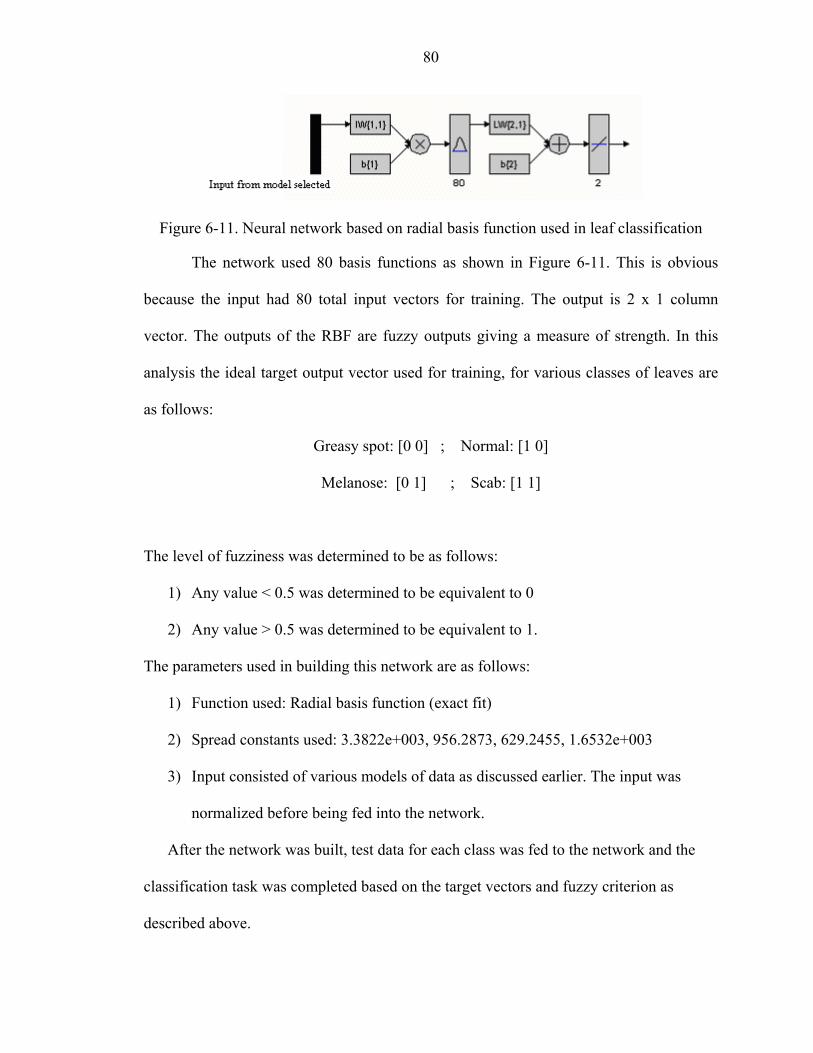
80
Figure 6-11. Neural network based on radial basis function used in leaf classification
The network used 80 basis functions as shown in Figure 6-11. This is obvious
because the input had 80 total input vectors for training. The output is 2 x 1 column
vector. The outputs of the RBF are fuzzy outputs giving a measure of strength. In this
analysis the ideal target output vector used for training, for various classes of leaves are
as follows:
Greasy spot: [0 0] ; Normal: [1 0]
Melanose: [0 1] ; Scab: [1 1]
The level of fuzziness was determined to be as follows:
1) Any value < 0.5 was determined to be equivalent to 0
2) Any value > 0.5 was determined to be equivalent to 1.
The parameters used in building this network are as follows:
1) Function used: Radial basis function (exact fit)
2) Spread constants used: 3.3822e+003, 956.2873, 629.2455, 1.6532e+003
3) Input consisted of various models of data as discussed earlier. The input was
normalized before being fed into the network.
After the network was built, test data for each class was fed to the network and the
classification task was completed based on the target vectors and fuzzy criterion as
described above.

CHAPTER 7 RESULTS
The results for the various classification strategies that were used are given below:
Generalized Square Distance Classifier from SAS
Model Color Feature Greasy spot Melanose Normal Scab Overall 1B HS 100 100 90 95 96.3 2B I 100 100 95 100 98.8 3B HSI 100 100 100 100 100 4B ALL 100 100 100 100 100
Table 7-1. Percentage classification results of the test data set from SAS
The results shown in Table 7-1 were obtained using a generalized square distance
classifier in SAS (PROC DISCRIM). The results were part of preliminary investigations
by Burks (2002). The results reported better classification accuracies for all the data
models. In particular, models 3B and 4B achieved perfect overall classification rates.
Model 1B achieved an overall accuracy of 96.3 % and model 2B an accuracy of 98.8%.
However, it should be noted that models 2B, 3B and 4B involve calculation of intensity
texture features, which is disadvantageous in terms of computational complexity.
Therefore, it is deciphered that model 1B is the overall best model in this classifier.
One more advantage of using 1B is the decrease in computational time for training
and classification. This is because of the elimination of intensity features and because of
the less number of features present in the model.
81

82
Statistical Classifier Based on Mahalanobis Minimum Distance Principle
Model Color Feature Greasy spot Melanose Normal Scab Overall 1B HS 100 100 100 95 98.75 2B I 100 95 95 100 97.5 3B HSI 0 100 100 100 75 4B ALL 90 100 80 60 85
Table 7-2. Percentage classification results for mahalanobis distance classifier
The results shown in Table 7-2 were obtained using the Mahalanobis minimum
distance classifier. In particular, models 1B and 2B achieved better overall classification
rates. Model 1B achieved an overall accuracy of 98.75 % and model 2B an accuracy of
97.5%. However, it should be noted that model 2B involves calculation of intensity
texture features as already explained in the above paragraphs. Therefore, model 1B is the
overall best model in this classifier.
In general, tables 7.1 and 7.2 prove that the results for both classifiers based on
statistical classification agree closely, especially concerning models 1B and 2B. Although
model 2B performed well in both cases, it is not useful in real world applications, since
choosing only intensity may be detrimental to the classification task due to inherent
intensity variations in an outdoor lighting environment. Hence, model 1B emerges as the
best model in classifiers based on statistical classification.
Neural Network Classifier Based on Feed Forward Back Propagation Algorithm
Model Color Feature Greasy spot Melanose Normal Scab Overall 1B HS 100 90 95 95 95 2B I 95 95 15 100 76.25 3B HSI 100 90 95 95 95 4B ALL 100 95 100 100 98.75
Table 7-3. Percentage classification results for neural network using back propagation

83
The results shown in Table 7.3 were obtained using Neural Network based on Back
Propagation principle. In particular, models 1B, 3B and 4B achieved better overall
classification rates. Models 1B and 3B achieved an overall accuracy of 95 % and model
4B an accuracy of 98.75%. Based on the explanation already given model 1B emerged as
the best model in this classification strategy.
Neural Network Classifier Based on Radial Basis Functions
Model Color Feature Greasy spot Melanose Normal Scab Overall 1B HS 100 100 85 60 86.25 2B I 100 20 75 0 48.75 3B HSI 95 80 85 85 86.25 4B ALL 100 95 100 95 97.5
Table 7-4. Percentage classification results for neural network using RBF
The results shown in Table 7.4 were obtained using Neural Network based on
Radial Basis Functions (RBF). In particular, models 1B, 3B and 4B achieved better
overall classification rates. Models 1B and 3B achieved an overall accuracy of 86.25%
and model 4B an accuracy of 97.5%.
Model 4B achieved higher overall classification accuracy. It is justifiable since
model 4B consists of more texture features, which is beneficial in neural network
applications, which are curve-fitting problems. However, in an outdoor application model
4B may be disadvantageous due to the large CPU calculation time required in calculating
the texture features.
Therefore, from the experiments, it is concluded that model 1B consisting of
features from hue and saturation is the best model for the task of citrus leaf classification.
Elimination of intensity in texture feature calculation is the major advantage since it

84
nullifies the effect of light variability. In addition, algorithms would be faster due to the
less number of texture features (10) required.
Discussion. Burks (2002) completed preliminary investigations, for the task of
citrus leaf classification. In that study, the data sets consisted of both the front portion as
well as the back portion of leaves. From those data sets, the texture features for various
models as described earlier were obtained. The classification results using the SAS
generalized square distance classifier gave similar overall accuracies for both the front as
well as the back data models. However, in the case of back portion the accuracies were a
little bit higher. Hence, for this study it was decided to use the back portion of leaves for
feature extraction of various data models.
It is evident from Table 7.2 that, for models 3B and 4B, the classification
accuracies for some classes of leaves were inconsistent with the excellent results that
were obtained for other models. Mahalanobis distance method determines the similarity
of a set of values from an unknown sample (test data) to a set of values measured from a
collection of known samples (training data). For models 3B and 4B, it may be the case
that the spectrums for training and test were dissimilar for the particular choice of texture
features in those models. Since the classification was predominantly based on the
minimum distance, even a slight off bound may significantly affect the test accuracies.
Therefore, the choice of the model and hence the texture features selected, significantly
affect the classification results.
Similarly, from Tables 7.3 and 7.4, the results for neural network classifiers also
show some discrepancies in terms of accuracies for some models. In the case of neural
network with back propagation as well as with radial basis functions, model 2B (with

85
only intensity features) performs poorly. This can be attributed to the fact that the
network did not have enough information (in other words, there was overlapping of data
clusters) to make a perfect classification hyperplane to separate the data clusters
belonging to various classes of leaves. The intensity of the leaves when considered as a
whole may not have incorporated enough information, for the network to make correct
classification decisions. This proves the fact that for neural network classifiers using only
intensity texture features will not yield good classification. One significant point to be
noted in neural network classifiers is that the results may not be consistent across several
trials using the same input and parameters. This is because the weight initialization in the
network is random. Hence, the outputs vary. The results for neural network classifiers
that were shown in this research were the average of outputs (classification accuracies)
for three successive trials.
Model 1B emerged as the best model among various models. It was noted earlier,
that this was in part because of the elimination of the intensity texture features.
Elimination of intensity is advantageous in this study because it nullifies the effect of
intensity variations. Moreover, it reduces the computational complexity by foregoing the
need to calculate the CCM matrices and texture statistics for the intensity pixel map.
However, in an outdoor application, elimination of intensity altogether may have an
effect on the classification, since the ambient variability in outdoor lighting is not taken
into consideration. Hence, future research for outdoor applications should consider
outdoor lighting variability.
Table 7-5 shows the number of leaf samples classified into each category for the
case of a neural network classifier with back propagation algorithm using model 1B. The

86
results show that a few samples from melanose, normal and scab leaves were
misclassified. For the case of melanose infected leaves, two test images were
misclassified. One leaf sample was misclassified as belonging to normal leaf class and
the other as a scab infected leaf. Similarly, in the case of normal and scab images, one
test image form each class was misclassified as belonging to the other class. In general, it
was observed in various trials that misclassifications mainly occurred in three classes
namely melanose, normal and scab.
From Species Greasy spot Melanose Normal Scab Accuracy Greasy spot 20 0 0 0 100 Melanose 0 18 0 0 90 Normal 0 1 19 1 95
Scab 0 1 1 19 95
Table 7-5. Classification results per class for neural network with back propagation Figures 1-1 through 1-4 show the leaf samples belonging to various classes. It is
obvious that leaves belonging to melanose, normal and scab classes showed significant
difference form greasy spot leaves in terms of color and texture. The leaves belonging to
these three classes had minute differences as discernible to the human eye, which may
justify the misclassifications as shown in table 7-5. The false positives that were observed
in these leaves may be because for some test images, the feature set for the model chosen,
overlapped with the feature set of leaves belonging to other classes.
Table 7-6 lists the overall classification results for various classifiers for the
particular case of model 1B. The classification accuracies for each of the four classes of
leaves, using various classifiers, are shown in the table.

87
Classifier Greasy spot Melanose Normal Scab Overall SAS 100 100 90 95 96.3
Mahalanobis 100 100 100 95 98.75 NNBP 100 90 95 95 95 RBF 100 100 85 60 86.25
Table 7-6. Comparison of various classifiers for model 1B
The table serves as a benchmark in comparing the efficacy of various classifiers.
The overall accuracies are well above 95% for statistical classifiers as well as for neural
network classifier using the back propagation algorithm. Radial basis function (RBF)
network, achieved an overall accuracy of 86.25%. Since the RBF network is a curve
fitting problem in a higher dimensional space, the low accuracy may be attributed to the
fact that due to some overlap among the various data clusters, the classification may have
had some false positives as well as false negatives thus affecting the overall accuracy.

CHAPTER 8 SUMMARY AND CONCLUSIONS
A detailed study was completed to investigate the use of computer vision and
image processing techniques in agricultural applications. The task of citrus leaf disease
classification using the above mentioned techniques was successfully implemented.
Three different classes of citrus diseases: greasy spot, melanose and scab were used for
this study. The image data of the leaves selected for this study was collected using a
JAI MV90, 3 CCD color camera with 28-90 mm zoom lens. Algorithms for feature
extraction and classification based on image processing techniques were designed. The
feature extraction process used color co-occurrence methodology (CCM method). It is
a method, in which both the color and texture of an image are taken into account, to
arrive at unique features, which represent that image. The manual feeding of the
datasets, in the form of digitized RGB color photographs was implemented for feature
extraction and training the SAS statistical classifier. After training the SAS classifier,
the test data sets were used to analyze the performance of accurate classification. The
whole procedure of analysis was replicated for three alternate classification approaches
to include; statistical classifier using the Mahalanobis minimum distance method,
neural network based classifier using the back propagation algorithm and neural
network based classifier using radial basis functions.
The analyses prove that such methods can be used for agricultural applications in
areas such as precision farming. Model 1B emerged as the best data model for the task
of citrus leaf classification. The statistical classifiers gave good results averaging above
88

89
95% overall classification accuracy. Similarly, neural network classifiers also achieved
comparable results.
This research was a feasibility analysis to see whether the techniques investigated
in this research can be implemented in outdoor applications. The results that were
obtained prove that these methods can indeed be used for such applications. However,
it should be kept in mind that all the analyses in this study were done in controlled
laboratory conditions. The real world conditions are much more different due to the
inherent variability in natural outdoor lighting and tree structure. That would be a major
challenge to overcome in future implementations so as to make the research portable
for real time leaf classification.
Future work. The future implementations of the present research would include
analyzing disease conditions of the citrus trees in an outdoor environment. Moreover, the
tree canopy as a whole could be taken into consideration instead of just leaves.
Specifically, the research would include the study of tree canopies to determine the
presence of any disease condition. The whole technology could be incorporated onboard
an autonomous vehicle with GPS. This would not only identify the diseased trees but also
map out their positions in the grove so that selective chemical application is possible.
However, the above task is complex in terms of implementation due to the high
variability in outdoor conditions. The present research should be modified, to make it
feasible for outdoor applications, before such a system could be implemented.

APPENDIX A MATLAB CODE FILES
1) Mahalanobis minimum distance classifier to identify diseased citrus leaves from normal leaves. %% %%%%%%%%%%%%%%%%%%%%%%%%%%%%%%%%%%%%%%%% %% Citrus Disease Identification Project %% Agricultural & Biological engineering department %% UNIVERSITY OF FLORIDA %% Matlab program developed by Rajesh Pydipati, RESEARCH ASSISTANT (Ag & %%Bio Eng) %%%%%%%%%%%%%%%%%%%%%%%%%%%%%%%%%%%%%%%%%% %% g1.txt contains a 20 x n matrix where each row represents the n HSI features of the 20 training images of greasy spot leaves %% %% m1.txt contains a 20 x n matrix where each row represents the n HSI features of the 20 training images of melanose leaves %% %% n1.txt contains a 20 x n matrix where each row represents the n HSI features of the 20 training images of normal leaves %% %% s1.txt contains a 20 x n matrix where each row represents the n HSI features of the 20 training images of scab leaves %% %% In the 'testinputdata.txt'file the 20xn matrix of the test dataset should be input. Each row represents the n features of an image%% a=load ('g1.txt'); % greasy spot features are input here x=a'; %get the transpose to ease calculations s=size(x); m1=sum(x,2)/s(2); % find the mean vector(39x1) for greasy spot for i=1:20 x1(:,i)=x(:,i)-m1; end w=zeros(39,39); for i=1:20 w=w+((x1(:,i))*(x1(:,i))'); end cv1=w/s(2); % 39x39 covariance matrix for greasy spot b=load('m1.txt'); % melanose features are input here y=b'; t=size(y); m2=sum(y,2)/t(2); % mean vector(39x1) for melanose for i=1:20 y1(:,i)=y(:,i)-m2;
90

91
end w1=zeros(39,39); for i=1:20 w1=w1+((y1(:,i))*(y1(:,i))'); end cv2=w1/t(2); % covariance for melanose(39x39) c=load('n1.txt'); %normal leaf features are input here z=c'; u=size(z); m3=sum(z,2)/u(2); % 39x1 mean vector for normal leaf class for i=1:20 z1(:,i)=z(:,i)-m3; end w2=zeros(39,39); for i=1:20 w2=w2+((z1(:,i))*(z1(:,i))'); end cv3=w2/u(2); % covariance(39x39) for normal leaf class d=load('s1.txt'); % scab features are input here v=d'; o=size(v); m4=sum(v,2)/o(2); % mean vector (39x1) for scab for i=1:20 v1(:,i)=v(:,i)-m4; end w3=zeros(39,39); for i=1:20 w3=w3+((v1(:,i))*(v1(:,i))'); end cv4=w3/o(2); % covariance for scab count1=0; count2=0; count3=0; count4=0; greasyspot=0; melanose=0; normal=0; scab=0; tes=load('testinputdata.txt'); % test data features for a particular class say normal or scab etc are input here as a 20x39 matrix test=(tes)'; for i=1:20 warning off ma1i=abs(((test(:,i)-m1)')*(inv(cv1))*((test(:,i)-m1))); % mahalanobis distance from feature set of test image to greasyspot class warning off

92
ma2i=abs(((test(:,i)-m2)')*(inv(cv2))*((test(:,i)-m2))); % mahalanobis distance from feature set of test image to melanose class warning off ma3i=abs(((test(:,i)-m3)')*(inv(cv3))*((test(:,i)-m3))); % mahalanobis distance from feature set of test image to normal leaf class warning off ma4i=abs(((test(:,i)-m4)')*(inv(cv4))*((test(:,i)-m4))); % mahalanobis distance from feature set of test image to scab class warning off ns=[ma1i ma2i ma3i ma4i]; mp=min(ns); % find the minimum mahalanobis distance and classify accordingly if mp==ma1i class=1; count1=count1+1; else if mp==ma2i class=2; count2=count2+1; else if mp==ma3i class=3; count3=count3+1; else class=4; count4=count4+1; end end end end greasyspot=count1; melanose=count2; normal=count3; scab=count4; greasyspot % number of test images classified as greasyspot diseased leaf melanose % number of test images classified as melanose diseased leaf normal % number of test images classified as normal leaf scab % number of test images classified as scab diseased leaf

93
2) Neural network classifier based on back propagation algorithm
%% %%%%%%%%%%%%%%%%%%%%%%%%%%%%%%%%%%%%%%%% %% Citrus Disease Identification Project %% Agricultural & Biological engineering department %% UNIVERSITY OF FLORIDA %% Matlab program developed by Rajesh Pydipati, RESEARCH ASSISTANT (Ag & %%Bio Eng) %%%%%%%%%%%%%%%%%%%%%%%%%%%%%%%%%%%%%%%%%%
%% Model studied here is model 4B clear a= load('train.txt'); b= load('test.txt'); d = load(‘dd.txt’); tp1=flipud(rot90(a)); tp2=flipud(rot90(b)); tt1=d'; h1=[20 15 10 8]; h11=15; h12=15; input_size=size(tp1,1); for i=1:input_size ip1(i,:)=tp1(i,:)/(max(tp1(i,:))); end clear tp1; for i=1:input_size ip2(i,:)=tp2(i,:)/(max(tp2(i,:))); end clear tp2; for i=1:4 sprintf('Trail %d',i) h11 = h1(i); h12=h1(i); net = newff(minmax(ip1),[h11 h12 4],{'tansig' 'tansig' 'tansig' }); net.trainParam.epochs = 3000; net.trainParam.goal = 0.0000001; [net,tr]= train(net, ip1, tt1); aout = sim(net,ip2); class1=aout(:,1:20); class2=aout(:,21:40); class3=aout(:,41:60); class4=aout(:,61:80); [max1,win1] = max(class1); specie1=zeros(4); for i=1:20

94
if win1(i)==1 specie1(1)= specie1(1)+1; elseif win1(i) == 2 specie1(2)= specie1(2)+1; elseif win1(i) == 3 specie1(3)= specie1(3)+1; elseif win1(i) == 4 specie1(4)= specie1(4)+1; end end specie1 grespotacc=specie1(1)/20*100 [max2,win2] = max(class2); specie2=zeros(4); for i=1:20 if win2(i)==1 specie2(1)= specie2(1)+1; elseif win2(i) == 2 specie2(2)= specie2(2)+1; elseif win2(i) == 3 specie2(3)= specie2(3)+1; elseif win2(i) == 4 specie2(4)= specie2(4)+1; end end specie2 melacc=specie2(2)/20*100 [max3,win3] = max(class3); specie3=zeros(4); for i=1:20 if win3(i)==1 specie3(1)= specie3(1)+1; elseif win3(i) == 2 specie3(2)= specie3(2)+1; elseif win3(i) == 3 specie3(3)= specie3(3)+1; elseif win3(i) == 4 specie3(4)= specie3(4)+1; end end specie3 noracc=specie3(3)/20*100 [max4,win4] = max(class4); specie4=zeros(4); for i=1:20 if win4(i)==1

95
specie4(1)= specie4(1)+1; elseif win4(i) == 2 specie4(2)= specie4(2)+1; elseif win4(i) == 3 specie4(3)= specie4(3)+1; elseif win4(i) == 4 specie4(4)= specie4(4)+1; end end specie4 scabacc=specie4(4)/20*100 end

APPENDIX B MINIMIZATION OF COST FUNCTION
As is well known from elementary calculus, to find an extremum of a function the
procedure is :
1. differentiate the function with respect to the free variable(s),
2. equate the result(s) with zero, and
3. solve the resulting equation(s).
In the case of least squares applied to supervised learning with a linear model the
function to be minimised is the sum-squared-error
(b.1)
where
(b.2)
and the free variables are the weights .
The minimum of the cost function
96

97
(b.3)
used in ridge regression would be shown in the paragraphs below. The cost function
includes an additional weight penalty term controlled by the values of the non-negative
regularisation parameters, . To get back to ordinary least squares (without any
weight penalty) is simply a matter of setting all the regularisation parameters to zero.
The optimisation for the j-th weight involves the following steps:
First, differentiating the cost function yields:
(b.4)
In the above equation the derivative of the model which, because the model is linear, is
particularly simple and is given as
(b.5)
Substituting this into the derivative of the cost function and equating the result to zero
leads to the equation
(b.6)

98
There are m such equations, for , each representing one constraint on the
solution. Since there are exactly as many constraints as there are unknowns the system of
equations has, except under certain pathological conditions, a unique solution.
To find that unique solution we employ the language of matrices and vectors: linear
algebra. These are invaluable for the representation and analysis of systems of linear
equations like the one above which can be rewritten in vector notation as follows.
(b.7)
where
(b.8)
Since there is one of these equations (each relating one scalar quantity to another) for
each value of j from 1 up to m we can stack them, one on top of another, to create a
relation between two vector quantities.
(b.9)
However, using the laws of matrix multiplication, this is just equivalent to

99
(b.10)
where
(b.11)
and where , which is called the design matrix, has the vectors as its columns,
and has p rows, one for each pattern in the training set. Written out in full it is
(b.12)
The vector can be decomposed into the product of two terms, the design matrix and the
weight vector, since each of its components is a dot-product between two m-dimensional
vectors. For example, the i-th component of when the weights are at their optimal values
is
(b.13)

100
where
Note that while is one of the columns of , is one of its rows. is the result of
stacking the one on top of the other, or
(b.14)
Finally, substituting this expression for into the previous equation gives
the solution to which is
(b.15)
which is where the normal equation comes from.
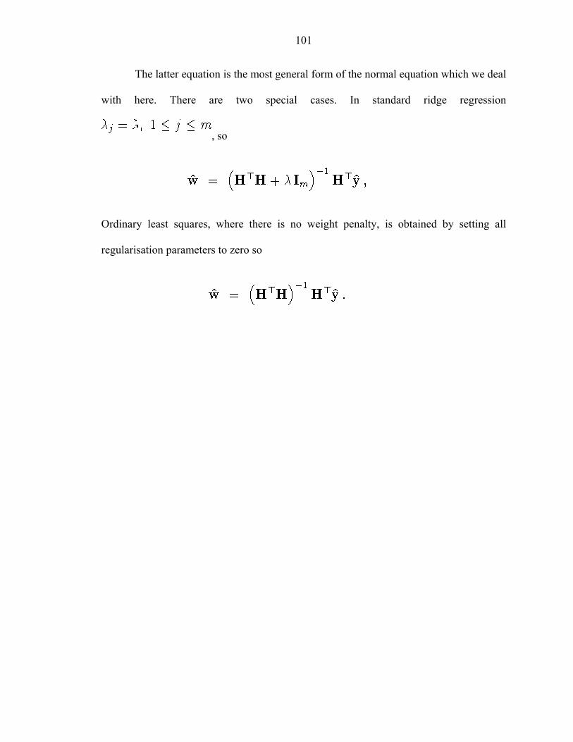
101
The latter equation is the most general form of the normal equation which we deal
with here. There are two special cases. In standard ridge regression
, so
Ordinary least squares, where there is no weight penalty, is obtained by setting all
regularisation parameters to zero so

LIST OF REFERENCES
Ampazis N. 1999. Introduction to neural networks, Artificial neural networks laboratory, Greece, http://www.iit.demokritos.gr/neural/intro (Accessed July 14, 2004).
Burks, T.F. 2002. Early detection of citrus diseases using machine vision. Presentation at ASAE conference. Chicago, USA. 2002.
Burks, T.F., S.A. Shearer, and F.A. Payne. 2000a. Classification of weed species using color texture features and discriminant analysis. Transactions of ASAE, Volume 43(2), Page(s), 441:448.
Burks, T.F., S.A. Shearer, R.S. Gates, and K.D. Donohue. 2000b. Backpropogation neural network design and evaluation for classifying weed species using color image texture. Transactions of ASAE, Volume 43(4), Page(s), 1029:1037.
Clark, C.J., V.A. McGlone, and R.B. Jordan. 2003. Detection of brownheart in braeburn apple by transmission NIR spectroscopy. Elsevier science transactions on post-harvest biology and technology, Volume 28(1), April 2003, Page(s), 87:96.
Coggins, J. M., A framework for texture analysis based on spatial filtering, Ph.D. Dissertation, Computer Science Department, Michigan State University, East Lansing, Michigan, 1982.
Edwards, J.G., and C.H.Sweet. 1986. Citrus blight assessment using a microcomputer; quantifying damage using an apple computer to solve reflectance spectra of entire trees. Florida Scientist, Volume 49(1), Page(s), 48:54.
Franz, E., M.R. Gebhardt, and K.B. Unklesbay. 1991. The use of local spectral properties of leaves as an aid for identifying weed seedlings in digital images. Transactions of ASAE, Volume 34(20), Page(s), 682:687.
Guyer, D.E., G.E. Miles, D.L. Gaultney, and M.M. Schreiber .1993. Application of machine vision to shape analysis in leaf and plant identification. Transactions of ASAE, Volume 36(1), Page(s), 163:171.
Guyer, D.E., G.E. Miles, M.M. Schreiber, O.R. Mitchell, and V.C. Vanderbilt. 1986. Machine vision and image processing for plant identification. Transactions of ASAE, Volume 29(6), Page(s), 1500:1507.
Hatfield, J.L., and P.J. Pinter, Jr. 1993. Remote sensing for crop protection. Crop Protection. Volume 12(6), Page(s), 403:414.
102

103
Haralick, R., K. Shanmugam, I. Dinstein. 1973. Texture features for image classification, IEEE Transactions on Systems, Man, and Cybernetics,Volume(3), Page(s), 610:621.
Hodges, A., E. Philippakos, D. Mulkey, T. Spreen, and R. Muraro. 2001. Economic impact of Florida’s citrus industry. University of Florida,Gainesville. IFAS publications. Economic information report 01-2.
Jain, A.K., and M. Tuceryan. 1998. Texture Analysis, In the handbook of pattern recognition and computer vision (2nd Edition), by C. H. Chen, L. F. Pau, P. S. P. Wang (eds.), Page(s), 207-248, World Scientific Publishing Co., Singapore(Book Chapter).
Kataoka, T., O. Hiroshi, and H. Shun-ichi. 2001. Automatic detecting system of apple harvest season for robotic apple harvesting. Presented at the 2001 ASAE Annual international meeting, Sacramento, California. Paper No. 01-3132.
Kim, M.S., Y.R. Chen, and P.M. Mehl. 2001. Hyperspectral reflectance and fluorescence imaging system for food quality and safety. Transactions of ASAE, Volume 44(3), Page(s), 721:729.
Chao, K., Y.R. Chen, and M. S. Kim. 2002. Machine vision technology for agricultural applications. Elsevier science transactions on computers and electronics in agriculture, Volume 36(2-3), November 2001, Page(s), 173:191.
Laws, K. I., 1980. Textured image segmentation. Ph.D. Dissertation, University of Southern California.
Lee, W.S, and D. Slaughter. 1998. Plant recognition using hardware-based neural network. Presented at the 1998 ASAE Annual international meeting, Orlando, Florida. Paper No. 983040.
Mark J.L. Orr. 1996. Introduction to radial basis function networks, Center for cognitive science, Edinburgh, Scotland, http://www.anc.ed.ac.uk/~mjo/intro/intro.html (Accessed July 14, 2004).
Moshou, D., H. Ramon, and J. De Baerdemaeker. 2002. A weed species spectral detector based on neural networks, Precision Agriculture Journal, Volume 3(3), Page(s), 209-223.
Nakano, K. 1998. Application of neural networks to the color grading of apples. Computers and electronics in agriculture, Volume 14, Page(s), 105-116.
Ninoyoma, S and I. Shigemori. 1991. Quantitative evaluation of soybean plant shape by image analysis. Japan. J. Breed, Volume 41, Page(s), 485:497.
Ning, K., M. Zhang, R. Ruan, and P.L. Chen, 2001. Computer vision for objective inspection of beans quality. Presented at the 2001 ASAE Annual international meeting, Sacramento, California. Paper No. 01-3059.
104
Pearson, T and R. Young. 2001. Automated sorting of almonds with embedded shell by laser transmittance imaging. ASAE Annual international meeting, Sacramento, California. Paper No. 01-013099.
Slaughter, D.C. 1987. Color vision for robotic orange harvesting. PhD Dissertation submitted to the University of Florida, Gainesville.
Tang, L., L.F. Tian, B.L. Steward, and J.F. Reid. 1999. Texture based weed classification using gabor wavelets and neural networks for real time selective herbicide applications. ASAE/CSAE-SCGR Annual international meeting, Toronto, Canada. Paper No. 993036.
Thompson, J.F., J.V. Stafford, and P.C.H. Miller. 1991. Potential for automatic weed detection and selective herbicide application. Crop Protection. Volume 10, Page(s), 254-259.
Tian, L., D.C. Slaughter, and R.F. Norris. 2000. Machine vision identification of tomato seedlings for automated weed control. Transactions of ASAE, Volume 40(6), Page(s), 1761:1768.
Woebbecke, D.M., G.E. Meyer, K. Von Bargen, and D.A. Mortensen. 1995a. Shape features for identifying young weeds using image analysis. Transactions of ASAE, Sacramento, California Volume 38(1), Page(s), 271:281.
Woebbecke, D.M., G.E. Meyer, K. Von Bargen, and D.A. Mortensen. 1995b. Color indices for weed identification under various soil, residue, and lighting conditions. Transactions of ASAE, Volume 38(1), Page(s), 259:269.
Yang, C., S. Prasher, and J. Landry. 1998. Application of artificial neural networks to image recognition in precision farming. Presented at 1998 ASAE annual meeting, Orlando, Florida. Paper No. 983039.
Yang, T., Y.R. Chen, and X. Cheng. 2001. Infrared imaging and wavelet-based segmentation method for apple defect inspection. ASAE Annual international meeting, Sacramento, California. Paper No. 01-3109.
Zeuch, N. 1988. Applying Machine Vision. John Wiley & Sons, New York, NY.
Zhang, N., and C. Chaisattapagon. 1995. Effective criteria for weed identification in wheat fields using machine vision. Transactions of ASAE, Volume 38(3), Page(s), 965:974.

BIOGRAPHICAL SKETCH
Rajesh Pydipati was born in India in the state of Andhra Pradesh. He graduated
with honors from the college of engineering at Sri Krishna Devaraya University in India
with a bachelor’s degree in electrical and electronics engineering. He was mentioned in
the dean’s list having topped the university in the engineering stream. He then started his
graduate studies at the University of Florida working towards a dual master’s degree
program in the Departments of Electrical and Computer Engineering and Agricultural
and Biological Engineering. He was a member of the Agricultural Robotics and
Mechatronics Group (ARMg) in the Department of Agricultural and Biological
Engineering, where he worked as a research assistant under the guidance of Dr.Thomas
F. Burks. He is a member of Eta Kappa Nu honor society of electrical engineers and
Alpha Epsilon honor society of agricultural engineers. When not indulged in academic
pursuits he likes to spend his time on the tennis courts. He was a junior champion in the
sport of tennis in India and also represented his university in the national collegiate
competitions in India.
105