An under-relaxation factorcontrol method for acceleratingthe iteration convergence of flow

field simulationC.H. Min and W.Q. Tao

State Key Laboratory of Multiphase Flow in Power Engineering,School of Energy and Power Engineering, Xi’an Jiaotong University,

Xi’an, People’s Republic of China

Abstract

Purpose – This paper aims to accelerate the iteration convergence for elliptic fluid flow problems, sothat an under-relaxation factor control method is developed.

Design/methodology/approach – There should be an optimal under-relaxation factor that canresult in the equivalence of the global residual norms of momentum equation u and momentumequation v. The two residual norms of the momentum equations will be equivalent through controllingthe velocity under-relaxation factors, and then the iteration convergence can be accelerated. Twoexpressions ða ¼ ða 0Þb

g

and a ¼ ða 0Þð1=bÞg

Þ are proposed to adjust the values of under-relaxationfactors for every n iterations.

Findings – From the five preliminary computations it is found that the value of g can be larger than 1and of n can be less than 5 for an open system, and the value of g should be less than 1 and that of nshould be larger than 10 for a closed system. These two pairs of parameters are then used in anotherfive examples. It is found that the saving in CPU times is at least 43.9 percent for the closed system and67.5 percent for the open system.

Research limitations/implications – When the Re or Ra of the two-dimensional problems are low,this control method is feasible. More research work is needed in order to apply it in three-dimensionalor high Re or Ra problems.

Originality/value – This method is helpful for the acceleration of iteration convergence in simpleproblems, and is a preparation for the advanced research in complicated problems.

Keywords Simulation, Flow, Iterative methods

Paper type Research paper

NomenclatureA ¼ area of control-volume faceae, anb ¼ coefficients in the discretized

conservation equationsb ¼ source term in discretized

conservation equationsc ¼ constantD ¼ characteristic length of channel or

cavity

DIV ¼ divergenceG ¼ global residual normH ¼ heightL ¼ lengthn ¼ iteration number for the control

methodp ¼ pressurep* ¼ intermediate pressure

The current issue and full text archive of this journal is available at

www.emeraldinsight.com/0264-4401.htm

This work is supported by the National Natural Science Foundation of China (No. 50476046,50636050).

An under-relaxation factor

control method

793

Received 8 May 2006Revised 16 March 2007

Accepted 4 July 2007

Engineering Computations:International Journal for

Computer-Aided Engineering andSoftware

Vol. 24 No. 8, 2007pp. 793-813

q Emerald Group Publishing Limited0264-4401

DOI 10.1108/02644400710833314

p0 ¼ pressure correctionR ¼ residualRa ¼ Rayleigh numberRe ¼ Reynolds numberr ¼ radial coordinateT ¼ temperatureu, v ¼ velocity components in x and y

directionu*, v* ¼ intermediate velocityu0 v0 ¼ velocity correctionx, y ¼ spatial coordinatesa ¼ under-relaxation factorb ¼ exponent in equations (15)–(18)g ¼ exponent in equations (15)–(18)

1 ¼ pre-specified small value tocontrol convergence

r ¼ density

Subscriptsc ¼ lowest temperatureE, N, P ¼ grid pointse, n, p ¼ cell facesh ¼ highest temperaturein ¼ inletnb ¼ neighbor pointsp ¼ pressureu, v ¼ velocity components in x and y

direction

1. IntroductionIn numerical analysis of fluid flow and heat transfer problems, iterative methods arefrequently adopted in which velocity components are solved in segregated manner andthe linkage between velocity and pressure is ensured by the SIMPLE-series algorithm.Since, the leading iterative approach SIMPLE was proposed (Patankar and Spalding,1972), it has been widely applied in the fields of computational fluid dynamics (CFD)and numerical heat transfer (NHT). Over the past three decades, many variants such asSIMPLER, SIMPLEC, SIMPLEX and so on were developed, which consist the so-calledSIMPLE-family solution algorithms. During the development of the SIMPLE-familyalgorithms, how to accelerate the iteration convergence is one of the key problems forenhancing the solution algorithm.

In SIMPLE-family algorithms, the iteration convergence can be accelerated by threemethods (Tao, 2000). First, an explicit correction step for the velocities was suggested(Yen and Liu, 1993). By applying this explicit correction step to the SIMPLE, SIMPLECand PISO algorithms, significant reductions in the number of iterations and CPU timeto achieve convergence were demonstrated. The second method is to chooseappropriate values of the under-relaxation factors. Patankar (1980) pointed out that forthe SIMPLE algorithm the velocity under-relaxation factor of 0.5 and the pressureunder-relaxation of 0.8 were found to be satisfactory in a large number of fluid-flowcomputations. However, it is recommended that if the computational grid is notseverely nonorthogonal, the relation:

au þ ap ¼ c ð1Þ

gives almost the optimum result, where the constant c is 1 (Demirdzic et al., 1987) or 1.1(Peric, 1990). Later a pressure under-relaxation factor based on the minimization of theglobal residual norm of the momentum equations was proposed (Chatwani and Turan,1991). The procedure was applied to SIMPLE and SIMPLEC algorithms toautomatically select the pressure under-relaxation factor to minimize the globalresidual norm of the momentum equations at each iteration level, but a notable increasein convergence was not achieved. Some other researchers (Latimer and Pollard, 1985;Macarthur and Patankar, 1989; Marek and Straub, 1993) all stated the need for amethod of automatically optimizing the relaxation factors. Some new methods aredeveloped in recent years to accelerate the iteration convergence. For example, fuzzy

EC24,8

794

mathematics has been developed as a new branch of mathematics in the last 20 years.It is extensively applied in many fields of science and technology such as the control ofconvergence in CFD simulations (Ryoo et al., 1999; Dragojlovic et al., 2001). Later, thismethod was improved (Liu et al., 2002). On the other hand, a new algorithm SOARbased on the comparison between SIMPLE algorithm and the Newton-Raphsonmethod for automatically determining the optimum values of relaxation factors forSIMPLE algorithm was developed (Morii and Vierow, 2000). Recently, the SOARalgorithm and the SIMPLE algorithm for computing performance in collocated grid arecompared (Morii, 2005). The results showed that the SOAR had better computingperformance than that of SIMPLE as the grid is refined.

The other methods for different special cases are grouped into the third method. Forexample, the SIMPLE-family algorithms will converge slowly when there is rapidlyvarying pressure in flow field, such as flow through a blunt sampler and dust-ladenfluid flow through a paper filter. A method to improve the rate of the convergencefor the SIMPLE-family algorithms for such cases is proposed (Wen and Ingham,1993, 1994).

This paper gives a simpler method for the under-relaxation factor control based on anew idea for elliptic fluid flow simulation, which is different from the above-mentionedmethods. The discussion will focus on the 2D recirculating flows. By using theproposed method the two momentum equations can be iterated consistently throughcontrolling the velocity under-relaxation factor, and the iteration convergence can besignificantly accelerated. The feasibility of the proposed method is validated by tentypical examples.

2. Under-relaxation factor control method2.1 Criteria of iteration convergenceCommonly, for an open flow system which has both inflow and outflow boundaries, thecriterion for terminating the iteration of nonlinear computation is that the relativeresidual norm of the momentum equations is less than a pre-specified small value.For example, this pre-specified small value was 1 # 1 £ 1023 , 1 £ 1025 (Latimer andPollard, 1985). That is for momentum equation u, if following condition is satisfied:

Gu ¼

Pnode aeue 2

Pnbanbunb þ bþ Aeð pP 2 pE Þ

� �� �2� �1=2

ru2in # 1

ð2Þ

the convergence of u momentum equation is reached. In this paper, this pre-specifiedvalue is taken as small as 1 £ 1028.

For a closed system, a numerical integration can be made for the momentumequation along any section in the field to obtain the reference momentum shown in thedenominator of equation (2).

For a two-dimensional elliptic flow field, there are two norms of momentumequations of x direction and y direction, respectively, which are denoted by Gu and Gv.Therefore, the criteria for iteration convergence is:

maxðGu;GvÞ # 1 ð3Þ

An under-relaxation factor

control method

795

It usually takes much time to make the maximum of Gu and Gv to be less than the samepre-specified small value since the two values of Gu and Gv are not always in the sameorder.

2.2 Analysis of the existence of an optimum velocity under-relaxation factorFor the SIMPLE algorithm, the revised velocities in the correction step are:

u ¼ u*þ u0 v ¼ v*þ v0 p ¼ p*þ p0 ð4Þ

For momentum equation u, the residual is given by:

Ru ¼ aeue 2X

anbunb 2 b2 Aeð pP 2 pEÞ

¼ aeue 2X

anbunb 2 b2 Ae½ð p*P þ app

0P Þ2 ð p*E þ app

0E Þ�

¼ Ru;0 2 apAeð p0P 2 p0EÞ

ð5Þ

where:

Ru;0 ¼ aeue 2X

anbunb 2 b2 Aeð p*P 2 p*E Þ ð6Þ

A similar equation can be written for the v momentum equation. The global residualnorm is given by, therefore:

G ¼X

ðR2u þ R2

vÞ ð7Þ

Chatwani and Turan (1991) considered that G could be minimized with respect to theunder-relaxation factor for the pressure correction ap by setting the derivative to bezero. This leads to following equation for ap:

ap ¼

PRu;0Aeð p

0P 2 p0EÞ þ Rv;0Anð p

0P 2 p0N Þ

� �P

A2eð p

0P 2 p0E Þ

2 þ A2nð p

0P 2 p0N Þ

2h i ð8Þ

Assuming that the difference of the pressure corrections between two adjacent pointsis everywhere identical and is denoted by Dp0. The above equation for ap can berewritten as:

ap ¼

PðRu;0Ae þ Rv;0AnÞPðA2

eDp0 þ A2

nDp0Þ

ð9Þ

Combining the two residuals of the momentum equations with equation (8) thefollowing relations can be derived:

Ru ¼Ru;0

PA2

e 2 Ae

PðRu;0AeÞ þ Ru;0

PA2

n 2 Ae

PðRv;0AnÞP

ðA2e þ A2

nÞð10Þ

EC24,8

796

Rv ¼Rv;0

PA2

n 2 An

PðRv;0AnÞ þ Rv;0

PA2

e 2 An

PðRu;0AeÞP

ðA2e þ A2

nÞð11Þ

For a grid system with Ae ¼ An, assuming that the value of Ru,0 on all points areidentical, and the value of Rv,0 on all points are identical, too, we can get the followingrelation:

Ru ¼ 2Rv ¼

PðRu;0A

2nÞ2

PðRv;0AeAnÞP

ðA2e þ A2

nÞð12Þ

That is:

Gu ¼ Gv ð13Þ

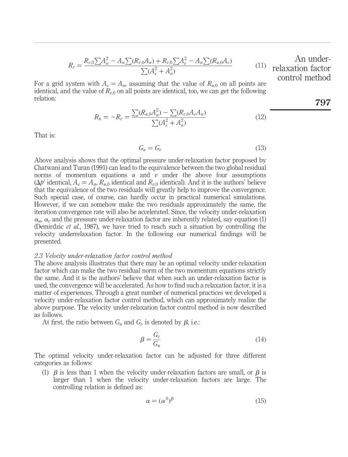
Above analysis shows that the optimal pressure under-relaxation factor proposed byChatwani and Turan (1991) can lead to the equivalence between the two global residualnorms of momentum equations u and v under the above four assumptions(Dp0 identical, Ae ¼ An, Ru,0 identical and Rv,0 identical). And it is the authors’ believethat the equivalence of the two residuals will greatly help to improve the convergence.Such special case, of course, can hardly occur in practical numerical simulations.However, if we can somehow make the two residuals approximately the same, theiteration convergence rate will also be accelerated. Since, the velocity under-relaxationau, av and the pressure under-relaxation factor are inherently related, say equation (1)(Demirdzic et al., 1987), we have tried to reach such a situation by controlling thevelocity underrelaxation factor. In the following our numerical findings will bepresented.

2.3 Velocity under-relaxation factor control methodThe above analysis illustrates that there may be an optimal velocity under-relaxationfactor which can make the two residual norm of the two momentum equations strictlythe same. And it is the authors’ believe that when such an under-relaxation factor isused, the convergence will be accelerated. As how to find such a relaxation factor, it is amatter of experiences. Through a great number of numerical practices we developed avelocity under-relaxation factor control method, which can approximately realize theabove purpose. The velocity under-relaxation factor control method is now describedas follows.

At first, the ratio between Gu and Gv is denoted by b, i.e.:

b ¼Gv

Guð14Þ

The optimal velocity under-relaxation factor can be adjusted for three differentcategories as follows:

(1) b is less than 1 when the velocity under-relaxation factors are small, or b islarger than 1 when the velocity under-relaxation factors are large. Thecontrolling relation is defined as:

a ¼ ða 0Þb ð15Þ

An under-relaxation factor

control method

797

where a is the velocity under-relaxation factor used for the present level, a 0 theunder-relaxation factor used in the previous iteration.

(2) b is larger than 1 when the under-relaxation factors are small, andb is less than 1when the under-relaxation factors are large. The controlling relation is defined as:

a ¼ ða0Þ1=b ð16Þ

(3) When the adoption of one of the above rules leads to a severe change in the velocityunder-relaxation factor, the iteration process may be deteriorated and even leadsto diverge. If this happens, i.e. the change of the velocity under-relaxation factor isover the given range (the upper limit of the velocity under-relaxation factor istaken as 0.98) with one of the two relations, the velocity under-relaxation factorshould be re-adjusted. This re-adjustment is very simple: use the other relationinstead of the one used before. That is, when use of the first relation leads toan acute variation of the velocity under-relaxation factor, then use the secondrelation to get a new value, and vice versa.

In order to further optimize the under-relaxation factor through the above tworelations, two more parameters, g and n, are introduced. The two relations, equations(15), (16) can be rewritten as:

a ¼ ða 0Þbg

ð17Þ

a ¼ ða 0Þð1=bÞg

ð18Þ

The value of g is always larger than zero. It is used to adjust the value of the exponent inthe two relations and enhance or alleviate the variation of the under-relaxation factorvalue between two iteration levels. For instance, the iteration may diverge with an acutevariation of the under-relaxation factor, and then reducing the value of g is helpful toalleviate this phenomenon. The value of b may change severely if we adjust theunder-relaxation factor each iteration, especially at the beginning of the iteration, whichmay decelerate the iteration convergence or even leads to the divergence of the iteration.So, we should adopt the method after several iterations from the beginning of thecomputation, then adjust the under-relaxation factor every n iterations. Additionally, toavoid the severe change of b, the range of b is given from 0.2 to 5.0. For a commonexample, the method can be adopted after 200 iterations from the beginning of thecomputation. Therefore, n is regarded as another parameter to enhance the convergence.From the following examples, we can see that an appropriate value ofn is very importantto the iteration convergence and some suggested value of n will be presented.

In the following presentation, the results of preliminary numerical tests will first bepresented, from which the values of g and n will be obtained through detail numericalpractices for five selected problems. Then these values are used in another five moreexamples directly, without any try and error computations. If the suggested values canstill lead to a significant saving of computational times for the five additionalexamples, then the feasibility of the proposed method can be considered justified insome extent. Fortunately, it is the case.

3. Preliminary test examplesFive flow and heat transfer problems (lid-driven cavity, flow in a 2D axisymmetricsudden expansion, flow over a backward-facing step, flow in annulus with the inner

EC24,8

798

wall rotating about the axis and natural convection in a square cavity) are used tovalidate the performance of the method and to find out the suggested values of g and n.The governing equations are discretized by the control volume method. The SIMPLECalgorithm is adopted to deal with the coupling between velocity and pressure, wherethe pressure correction under-relaxation factor is fixed at 1 (van Doormaal andRaithby, 1984; Tao, 2001). And the velocity under-relaxation factor is dealt with by theproposed control method. The pre-specified small value 1 is 1 £ 1028. Computationsare also conducted for au ¼ av ¼ 0.5 and the results by using these twounder-relaxation factors will be compared with the results obtained by adopting theproposed control method. We have tried different constants of au and av. The resultsshow that the computational CPU time is different under different initial values of au

and av. For different cases, the optimal values of au and av are also different. Hence, thesaving in CPU time are different by our method when different initial au and av areused. However, since for most cases people usually try to use au ¼ av ¼ 0.5 assuggested by Patankar, therefore, such practice is adopted in this paper. To comparethe CPU time between the velocity under-relaxation factor control method andau ¼ av ¼ 0.5 the relative time is adopted, i.e. for an example, the CPU time underau ¼ av ¼ 0.5 is divided by the CPU time under different cases.

3.1 Lid-driven cavityThe schematic of lid-driven cavity flow is shown in Figure 1. Computation is conductedfor Re ¼ 100 (Re ¼ UD/v), and the grid system used is 52 £ 52. Table I shows the CPUtime under different values of g and n. It can be observed that the saving in CPU time is

Figure 1.Lid-driven cavity

(Re ¼ 100)

x

y

U0=1, V=0

D

D

n 1 2 3 4 5 10 15 20 30 50 au ¼ 0.5

g ¼ 0.5 0.307 0.276 0.210 0.194 0.200 0.250 0.290 0.334 0.398 0.483 1g ¼ 0.8 0.301 0.328 0.276 0.231 0.201 0.213 0.244 0.274 0.328 0.403g ¼ 1.0 0.293 0.324 0.295 0.256 0.212 0.201 0.224 0.255 0.298 0.363g ¼ 1.2 0.326 0.325 0.307 0.269 0.237 0.191 0.209 0.238 0.282 0.339g ¼ 1.5 0.271 0.323 0.306 0.336 1.027 0.195 0.203 0.221 0.257 0.302

Table I.CPU time of lid–driven

cavity (s)

An under-relaxation factor

control method

799

80.9 percent with the appropriate value of g and n compares to au ¼ 0.5. The iterationcan converge under different value of n with the smaller value of g. When the value ofg becomes larger, the iteration is easy to be diverged. Additionally, Figure 2 shows therelationship between iteration times and under-relaxation factor with n ¼ 10. It can beobserved that when the value g is smaller, the variation of the under-relaxation factoris not significant. When the value of g becomes larger, the variation of theunder-relaxation factor becomes acute. Therefore, for this closed system, n is about 10and g can be larger than 1.

Figure 2.The relationship betweeniteration times andunder-relaxation factor

200 300 400 500 600 700 8000.4

0.5

0.6

0.7

0.8

0.9

iteration number

a u a u(a) g = 0.5

200 300 400 500 600 700

0.5

0.6

0.7

0.8

0.9

1.0

iteration number

(b) g = 0.8

200 300 400 500 600 7000.4

0.5

0.6

0.7

0.8

0.9

1.0

iteration number

a u

(c) g = 1.0

200 300 400 500 6000.4

0.5

0.6

0.7

0.8

0.9

1.0

iteration number

a u

(d) g = 1.2

(e) g = 1.5

200 300 400 500 600 7000.4

0.5

0.6

0.7

0.8

0.9

1.0

iteration number

a u

EC24,8

800

3.2 Flow in a 2D axisymmetric sudden expansionFigure 3 shows the schematic of flow in a 2D axisymmetric sudden expansion. Thesizes in computational region are Lx/Din ¼ 60, Lin/Din ¼ 10, D/Din ¼ 2. Re ¼ 150(Re ¼ UD/v). The grid system used is 102 £ 22. Table II shows the CPU time underdifferent values of g and n. It can be observed that the saving in CPU time is70.0 percent with the appropriate value of g and n compares to au ¼ 0.5. As shown inFigure 2 and 4, shows that the variation of the under-relaxation factor becomes acutewhen the value of g becomes larger and n ¼ 5. Additionally, we also find thatthe under-relaxation factor was over the given range in this example and it fell into thethird category described in the second section. So the under-relaxation factor wasre-adjusted. It is finally found that a larger value of g can accelerate the iterationconvergence. Thus, for this open system, g can be larger than 1, and n can be given bya relative small value.

3.3 Flow over a backward-facing stepThe schematic of flow over a backward-facing step is shown in Figure 5. The sizes incomputational region are Lx/H1 ¼ 60, Lin/H1 ¼ 10, H2/H1 ¼ 2. Re ¼ 100 (Re ¼ UD/v).The grid system used is 102 £ 32. Table III shows the CPU time under different valuesof g and n. It can be observed that the saving in CPU time is 74.3 percent with theappropriate value of g and n compared to au ¼ 0.5. Figure 6 shows the relationshipbetween iteration times and under-relaxation factor with n ¼ 5. The computationalresults of this example are similar to the computational results of flow in a 2Daxisymmetric sudden expansion.

3.4 Flow in annulus with the inner wall rotating about the axisThe schematic of flow in annulus with the inner wall rotating about the axis is shown inFigure 7. Re ¼ Uri/v ¼ 100. The grid system used is 52 £ 52. Table IV shows the CPUtime under different values of g and n. It can be observed that the saving in CPU time is

Figure 3.Schematic of flow in a 2D

axisymmetric suddenexpansion (Re ¼ 150)

x

r

Din

LRLin

Lx

D

n 1 2 3 4 5 10 15 20 30 50 au ¼ 0.5

g ¼ 0.5 0.309 0.325 0.362 0.382 0.395 0.403 0.409 0.405 0.428 0.429 1g ¼ 0.8 0.314 0.307 0.332 0.353 0.361 0.392 0.402 0.397 0.397 0.409g ¼ 1.0 DIV 0.306 0.320 0.330 0.341 0.391 0.397 0.394 0.384 0.426g ¼ 1.2 DIV 0.300 0.307 0.312 0.325 0.383 0.399 0.367 0.387 0.396g ¼ 1.5 DIV DIV DIV 0.310 0.321 0.372 0.351 0.342 0.391 0.407

Note: DIV – divergence

Table II.CPU time of flow in a 2D

axisymmetric suddenexpansion (s)

An under-relaxation factor

control method

801

43.9 percent with the appropriate value ofg andn compares toau ¼ 0.5. A smaller value ofg is good for accelerating the iteration convergence. Figure 8 shows the relationshipbetween iteration times and under-relaxation factor with n ¼ 10. When the value of g islarger than 1, the variation of the value of the under-relaxation factor is acute. So, for thisclosed system, the value of g should be less than 1, and n should be given by a relativelarge value.

Figure 4.The relationship betweeniteration times andunder-relaxation factor

a u

200 220 240 260 280 300 3200.0

0.2

0.4

0.6

0.8

1.0

iteration number

(b) g = 0.8

a u

200 240 280 320 3600.0

0.2

0.4

0.6

0.8

1.0

iteration number

(a) g = 0.5

a u

200 220 240 260 280 3000.0

0.2

0.4

0.6

0.8

1.0

iteration number

(c) g = 1

a u

200 220 240 260 280 3000.0

0.2

0.4

0.6

0.8

1.0

iteration number

(d) g = 1.2

a u

200 210 220 230 240 250 260 270 2800.0

0.2

0.4

0.6

0.8

1.0

iteration number

(e) g = 1.5

EC24,8

802

3.5 Natural convection in a square cavityThe schematic of natural convection in a square cavity is shown in Figure 9.Computation is conducted for Ra ¼ 104 (Ra ¼ r2gbDTD 3Pr/m2), and the grid systemused is 42 £ 42. Table V shows the CPU time under different values of g and n. It canbe observed that the saving in CPU time is 53.4 percent with the appropriate value of gand n compares to au ¼ 0.5. A smaller value of g is good for accelerating the iterationconvergence. Figure 10 shows the relationship between iteration times andunder-relaxation factor with n ¼ 10. It can be found that when the value of g issmall, the value of under-relaxation factor changes from small to large, and when thevalue of g becomes larger, the value of the under-relaxation factor becomes larger too.So, for this closed system, the value of g should be less than 1, and n should be given bya relative large value.

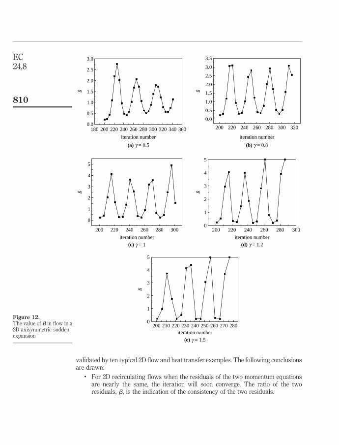
4. Application results and discussionAs discussed above, if the two residual modules of the momentum equations are in thesame order namely the value of b is nearly to be 1, the iteration will be easy to beconverged. Then the key issue is whether we can propose some values of g and n whichcan make b around 1 and, more important, are the proposed values common to a seriesof flow problems, so that one can directly adopt them in the flow computation withoutany preliminary test. We choose the lid-driven cavity flow and flow in a 2Daxisymmetric sudden expansion as the representatives of an open system and a closedsystem, respectively. The results of the effects of g on b for the two selectedrepresentative problems are shown in Figures 11 and 12, respectively. It can beobserved that for the two systems, the value of b is easy to be 1 when the value of g issmall, while with increasing g the approach of 1 for the value of b gradually

Figure 5.Schematic of flow over a

backward-facing step(Re ¼ 100)

Lx

Lin LR

H2

H1 x

y

n 1 2 3 4 5 10 15 20 30 50 au ¼ 0.5

g ¼ 0.5 DIV 0.257 0.278 0.295 0.303 0.324 0.335 0.334 0.347 0.342 1g ¼ 0.8 DIV DIV 0.262 0.262 0.279 0.304 0.325 0.314 0.331 0.317g ¼ 1.0 DIV DIV DIV 0.257 0.262 0.295 0.311 0.310 0.317 0.334g ¼ 1.2 DIV DIV DIV DIV 0.257 0.289 0.307 0.304 0.305 0.317g ¼ 1.5 DIV DIV DIV DIV 0.257 0.282 0.282 0.278 0.281 0.318

Note: DIV – divergence

Table III.CPU time of flow over abackward-facing step (s)

An under-relaxation factor

control method

803

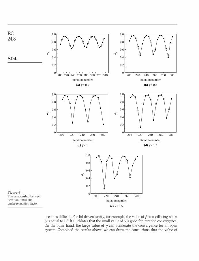
becomes difficult. For lid-driven cavity, for example, the value of b is oscillating wheng is equal to 1.5. It elucidates that the small value of g is good for iteration convergence.On the other hand, the large value of g can accelerate the convergence for an opensystem. Combined the results above, we can draw the conclusions that the value of

Figure 6.The relationship betweeniteration times andunder-relaxation factor

200 220 240 260 280 300 320 3400

0.2

0.4

0.6

0.8

1.0

iteration number

(a) g = 0.5 (b) g = 0.8

(c) g = 1 (d) g = 1.2

(e) g = 1.5

200 220 240 260 280 3000

0.2

0.4

0.6

0.8

1.0

iteration number

a ua u

a ua u

a u

200 220 240 260 2800

0.2

0.4

0.6

0.8

1.0

iteration number

200 220 240 260 2800

0.2

0.4

0.6

0.8

1.0

iteration number

200 220 240 260 2800

0.2

0.4

0.6

0.8

1.0

iteration number

EC24,8

804

g can be larger than 1 and of n can be less than 5 for an open system, and the value of gshould be less than 1 and of n should be larger than 10 for a closed system.

The method proposed by Chatwani and Turan (1991) accompanied with equation(13) is also adopted for the above five examples. It is found that by using this methodboth pressure under-relaxation and velocity under-relaxation are very unstable, whichmay even results in the iteration divergence. Thus, it seems that the method is notcommon for most other cases although it has a good character for some special casespresented in that paper.

In order to evaluate the feasibility of the proposed method, another five examples,such as natural convection in an annual cavity ðRa ¼ r 2gbDTðro 2 riÞ

3Pr =m 2 ¼ 104Þ;natural convection in a vertical annual pipe ðRa ¼ r 2gbDTðro 2 riÞ

3Pr =m 2 ¼ 104Þ;isolated island problem ðRa ¼ r 2gbDTD 3Pr =m 2 ¼ 105Þ; flow in a 2D axisymmetricfinned tube (Re ¼ UD/v ¼ 200, where D is the diameter of the tube) and flow over aparallel finned channel (Re ¼ UD/v ¼ 200, where D is the distance between the twoplate) are used to validate the method under the values ofg andnbasically obtained fromthe preliminary tests, and are fixed at 1.2 and 5, respectively, for the open system, and 1.0and 10, respectively, for closed system. The schematics of the five examples are shown inFigure 13 and the computational results are shown in Table VI. In the table, the CUPtimes required when au ¼ 0.5 are also shown.

Figure 7.Schematic of flow in

annulus with the innerwall rotating about the

axis (Re ¼ 100)

U=1.0

ri

n 1 2 3 4 5 10 15 20 30 50 au ¼ 0.5

g ¼ 0.5 0.810 0.635 0.596 0.594 0.586 0.611 0.629 0.657 0.874 0.816 1g ¼ 0.8 1.702 0.696 0.626 0.619 0.589 0.579 0.609 0.609 0.853 0.756 0g ¼ 1.0 4.613 0.737 0.678 0.632 0.628 0.561 0.617 0.585 0.858 0.734 0g ¼ 1.2 DIV 0.972 0.696 0.671 0.670 0.637 0.591 0.599 0.880 0.692 0g ¼ 1.5 1.203 1.488 0.792 0.688 0.773 0.682 0.577 0.667 0.903 0.663 0

Note: DIV – divergence

Table IV.CPU time of flow in

annulus with the innerwall rotating about the

axis (s)

An under-relaxation factor

control method

805

Table VI also shows the good performance of proposed method for theunder-relaxation factor control. Based on the above examples it may berecommended that for the proposed method the values of g and n are 1.2 and 5,respectively, for an open system and 1.0 and 10, respectively, for a closed system.

Figure 8.The relationship betweeniteration times andunder-relaxation factor

200 300 400 5000.2

0.3

0.4

0.5

0.6

0.7

0.8

0.9

1.0

iteration number

a u

150 200 250 300 350 400 450 5000.2

0.3

0.4

0.5

0.6

0.7

0.8

0.9

1.0

iteration number

a u

(a) g = 0.5 (b) g = 0.8

150 200 250 300 350 400 450 5000.2

0.3

0.4

0.5

0.6

0.7

0.8

0.9

1.0

iteration number

a u

(c) g = 1

(e) g = 1.5

(d) g = 1.2

200 300 400 500 6000.2

0.3

0.4

0.5

0.6

0.7

0.8

0.9

1.0

iteration number

a u

200 300 400 500 6000.2

0.3

0.4

0.5

0.6

0.7

0.8

0.9

1.0

iteration number

a u

EC24,8

806

Finally, the implementation of the proposed control methods is described here. In theprogram, the initial value of the velocity under-relaxation factor is 0.5, the given upperlimit of velocity under-relaxation factor is 0.98, and the given range of b is 0.2 to 5.0.After 200 levels from the beginning of the computation with SIMPLEC algorithm, itcomputes the value of b, and one of the relations (17) and (18) is adopted first to updatethe velocity under-relaxation factor. If the velocity under-relaxation factor is overthe given upper limit, the other relation is automatically used at the next update. In thesubsequent computation the velocity under-relaxation factor is updated for every niterations until the convergence is reached.

Finally, we would like to make some further discussion related to the initial fieldassumption and the application of the present method to 3D cases. First, it iswell-known that the initial fields strongly affect the iteration convergence (Patankar,1980; Tao, 2001). A good initial field can improve the iteration convergence. In thepresent work, the inlet condition is used as initial field for open systems, and for closedsystems the zero velocities in the computational domain are adopted as the initialfields. To the authors’ knowledge, such initial fields can be simply carried out andadopted easily by all researchers and no any specific techniques are required. And for

Figure 9.Schematic of natural

convection in a squarecavity (Ra ¼ 104)

x

y

D

D

TH TC

adiabatic

adiabatic

n 1 2 3 4 5 10 15 20 30 50 au ¼ 0.5

g ¼ 0.5 DIV 0.475 0.466 0.472 0.485 0.571 0.614 0.687 0.660 0.846 1g ¼ 0.8 DIV DIV DIV 0.468 0.474 0.527 0.547 0.627 0.550 0.775g ¼ 1.0 DIV DIV DIV 0.471 0.481 0.527 0.543 0.581 0.531 0.756g ¼ 1.2 DIV DIV 0.513 DIV 0.474 0.493 0.523 0.550 0.535 0.718g ¼ 1.5 DIV DIV 0.514 0.833 DIV 0.466 0.535 0.528 0.510 0.685

Note: DIV – divergence

Table V.CPU time of natural

convection in a squarecavity (s)

An under-relaxation factor

control method

807

such initial fields, our method works well. Thus, we believe that our method is usefulsince it can effectively converge the iteration by the very simple and straightforwardinitial field assumptions. As far as the three dimensional cases are concerned, there arethree global residual norms for 3D case. Whether the convergence will be accelerated ifthe residual norms of the three momentum equations are more or less equal and how to

Figure 10.The relationship betweeniteration times andunder-relaxation factor

200 250 300 350 400 450 500 5500.4

0.5

0.6

0.7

0.8

0.9

1.0

iteration number

a u

0.4

0.5

0.6

0.7

0.8

0.9

1.0

a u

(a) g = 0.5

200 250 300 350 400 450 500 5500.4

0.5

0.6

0.7

0.8

0.9

1.0

iteration number

a u

0.4

0.5

0.6

0.7

0.8

0.9

1.0

a u

(c) g = 1

200 250 300 350 400 450

iteration number

(d) g = 1.2

200 250 300 350 400 450

iteration number

(e) g = 1.5

200 250 300 350 400 450 500 550

iteration number

(b) g = 0.8

0.4

0.5

0.6

0.7

0.8

0.9

1.0

a u

EC24,8

808

apply the method for high Re or Ra cases, more research work is needed. And the workis underway in the authors’ group.

5. ConclusionsAn under-relaxation factor control method is developed to accelerate iterationconvergence of flow field computation. The good performance of this method is

Figure 11.The value of b inlid-driven cavity

200 300 400 500 600 700 8000.75

0.80

0.85

0.90

0.95

1.00

1.05

iteration number

ß

0.75

0.80

0.85

0.90

0.95

1.00

1.05

ß

(a) g = 0.5

(c) g = 1

(e) g = 1.5

200 300 400 500 600 700

iteration number

(b) g = 0.8

200 300 400 500 600 7000.75

0.80

0.85

0.90

0.95

1.00

1.05

1.10

iteration number

(d) g = 1.2

iteration number

ß

200 300 400 500 6000.6

0.7

0.8

0.9

1.0

1.1

1.2

1.3ß

200 300 400 500 600 7000.3

0.6

0.9

1.2

1.5

1.8

2.1

iteration number

ß

An under-relaxation factor

control method

809

validated by ten typical 2D flow and heat transfer examples. The following conclusionsare drawn:

. For 2D recirculating flows when the residuals of the two momentum equationsare nearly the same, the iteration will soon converge. The ratio of the tworesiduals, b, is the indication of the consistency of the two residuals.

Figure 12.The value of b in flow in a2D axisymmetric suddenexpansion

180 200 220 240 260 280 300 320 340 3600.0

0.5

1.0

1.5

2.0

2.5

3.0

iteration number

ß

200 220 240 260 280 300 320

0.0

0.5

1.0

1.5

2.0

2.5

3.0

3.5

ß

(a) g = 0.5

(c) g = 1

iteration number

(b) g = 0.8

200 220 240 260 280 300

0

1

2

3

4

5

iteration number

(e) g = 1.5

iteration number

ß

(d) g = 1.2

200 220 240 260 280 3000

1

2

3

4

5

iteration number

ß

200 210 220 230 240 250 260 270 2800

1

2

3

4

5

ß

EC24,8

810

. In order to make b being around 1, different relations are given for adjusting thevelocity under-relaxation factor. Two parameters g and b, are introduced inthe re-determination of the under-relaxation factor by equations (15) and (16).The adjustment of au should be conducted every n iterations.

. Preliminary tests show that the value of g can be larger than 1 and of n can beless than 5 for an open system, and the value of g should be less than 1 and of nshould be larger than 10 for a closed system. The two pairs of recommendedvalues are: g and n equal 1.2 and 5, respectively, for an open system and 1.0 and10, respectively, for a closed system.

. Five flow and heat transfer problems are used to validate the proposed method.When the proposed values of the two parameters are used, compared with

Figure 13.Schematic of another five

examples

Th

Tc

ro

ri

z

r

Tc

Th

(a) natural convection inan annual cavity

(b) natural convection in avertical annual pipe

(c) isolated island problem

x

r

x

y

(d) flow in a 2D axisymmetric finned tube (e) flow over a parallel finned channel

Example g n

CPU timeof the proposed

method au ¼ 0.5

CPUtime saved(percent)

Natural convection in an annual cavity 1.0 10 0.362 1 63.8Natural convection in a vertical annual tube 1.0 10 0.435 1 56.5Isolated island problem 1.0 10 0.455 1 54.5Flow in a 2D axisymmetric finned tube 1.2 5 0.186 1 81.4Flow over a parallel finned channel 1.2 5 0.146 1 85.4

Table VI.CPU time of the five

examples (s)

An under-relaxation factor

control method

811

au ¼ 0.5, the CPU time can be saved from 67.5 to 85.4 percent and from 43.9 to79.9 percent for an open system and for a closed system, respectively.

Finally, it should be noted that the proposed under-relaxation factor control methodcan be used for the elliptic problems, but not for the parabolic problems. And moreresearch work is needed in order to apply the method for high Re and Ra cases and 3Dsituations.

References

Chatwani, A.U. and Turan, A. (1991), “Improved pressure-velocity coupling algorithm based onminimization of global residual norm”, Numerical Heat Transfer, Part B, Vol. 20 No. 5,pp. 115-23.

Demirdzic, I., Gosman, A.D., Issa, R.I. and Peric, M. (1987), “A calculation procedure for turbulentflow in complex geometries”, Computers & Fluids, Vol. 15 No. 3, pp. 251-73.

Dragojlovic, Z., Kaminski, D.K. and Ryoo, J. (2001), “Tuning of a fuzzy rule set for controllingconvergence of a CFD solver in turbulent flow”, International Journal Heat and MassTransfer, Vol. 44 No. 20, pp. 3811-22.

Latimer, B.R. and Pollard, A. (1985), “Comparison of pressure-velocity coupling solutionalgorithms”, Numerical Heat Transfer, Part B, Vol. 8, pp. 635-52.

Liu, X.L., Tao, W.Q., Zheng, P., He, Y.L. and Wang, Q.W. (2002), “Control of convergence in acomputational fluid dynamic simulation using fuzzy logic”, Science in China (Series E),Vol. 45 No. 5, pp. 495-501.

Macarthur, J.W. and Patankar, S.V. (1989), “Robust semidirect finite difference methods forsolving the Navier-Stokes and energy equations”, International Journal of NumericalMethods in Fluids, Vol. 9, pp. 325-40.

Marek, R. and Straub, J. (1993), “Hybrid relaxation – a technique to enhance the rate ofconvergence of iterative algorithms”, Numerical Heat Transfer, Part B, Vol. 23 No. 4,pp. 483-97.

Morii, T. (2005), “A new efficient algorithm for solving an incompressible flow on relatively finemesh”, Numerical Heat Transfer, Part B, Vol. 47 No. 6, pp. 593-610.

Morii, T. and Vierow, K. (2000), “The SOAR method for automatically optimizing SIMPLErelaxation factors”, Numerical Heat Transfer, Part B, Vol. 38 No. 3, pp. 309-32.

Patankar, S.V. (1980), Numerical Heat Transfer and Fluid Flow, Hemisphere, Washington, DC,p. 128.

Patankar, S.V. and Spalding, D.B. (1972), “A calculation procedure for heat, mass and momentumtransfer in three-dimensional parabolic flows”, International Journal of Heat MassTransfer, Vol. 15 No. 10, pp. 1787-806.

Peric, M. (1990), “Analysis of pressure velocity coupling on nonorthogonal grids”, NumericalHeat Transfer, Part B, Vol. 17 No. 1, pp. 63-82.

Ryoo, J., Kaminski, D. and Dragojlovic, Z. (1999), “A residual-based fuzzy logic algorithm forcontrol of convergence in a computational fluid dynamic simulation”, ASME Journal ofHeat Transfer, Vol. 121, pp. 1076-8.

Tao, W.Q. (2000), Recent Advances in Computational Heat Transfer, Science Press, Beijing,pp. 166-9.

Tao, W.Q. (2001), Numerical Heat Transfer, 2nd ed., Xi’an Jitong University Press, Xi’an, p. 221.

van Doormaal, J.P. and Raithby, G.D. (1984), “Enhancement of the SIMPLE method for predictingincompressible fluid flow”, Numerical Heat Transfer, Vol. 7, pp. 147-63.

EC24,8

812

Wen, X. and Ingham, D.B. (1993), “A new method for accelerating the rate of convergence of theSIMPLE-like algorithm”, International Journal of Numerical Methods in Fluids, Vol. 17No. 5, pp. 385-400.

Wen, X. and Ingham, D.B. (1994), “A numerical method for accelerating the rate of convergenceof the SIMPLE-like algorithm for flow through a thin filter”, International Journal ofNumerical Methods in Fluids, Vol. 19 No. 10, pp. 889-903.

Yen, R.H. and Liu, C.H. (1993), “Enhancement of the SIMPLE algorithm by an additional explicitcorrection step”, Numerical Heat Transfer, Part B, Vol. 24 No. 1, pp. 127-41.

Corresponding authorW.Q. Tao can be contacted at: wqtao@mail.xjtu.edu.cn

An under-relaxation factor

control method

813

To purchase reprints of this article please e-mail: reprints@emeraldinsight.comOr visit our web site for further details: www.emeraldinsight.com/reprints